Multiphysics-Based Numerical Prediction of the Electromagnetic and Thermal Performance of a 160 kW SSDR Axial-Flux Motor

Abstract

Axial-flux motor (AFM) can achieve high torque and power density; however, integrated electromagnetic and thermal design is required to manage losses and heat generation during high-power operation. In this study, an AFM with a target output power of 160 kW for electric vehicles was analyzed using three-dimensional electromagnetic and thermal-fluid analyses. Electromagnetic analysis evaluated back EMF, cogging torque, torque, output power, efficiency, and losses. Current phase-angle control was applied at high speeds considering the 700 V line-to-line voltage limit of the 800 V inverter. At 300 A and 4500 rpm, the motor achieved an output power of 150 kW with an efficiency of approximately 94%. Electromagnetic losses were applied as heat sources in the thermal analysis. In the Base model, nonuniform oil flow caused local high-temperature regions. The model incorporating eight ribs in the oil-flow path and 12 rotor blades for enhanced air cooling reduced the maximum coil temperature from 194 °C to 170 °C and the maximum stator temperature from 205 °C to 113 °C. The model reduced the standard deviations of coil and stator temperatures by 50.6% and 58.6%, respectively. The proposed multi-physics method predicts electromagnetic and thermal characteristics and supports operating control and cooling system design.

1. Introduction

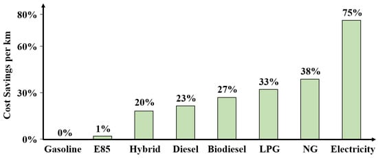
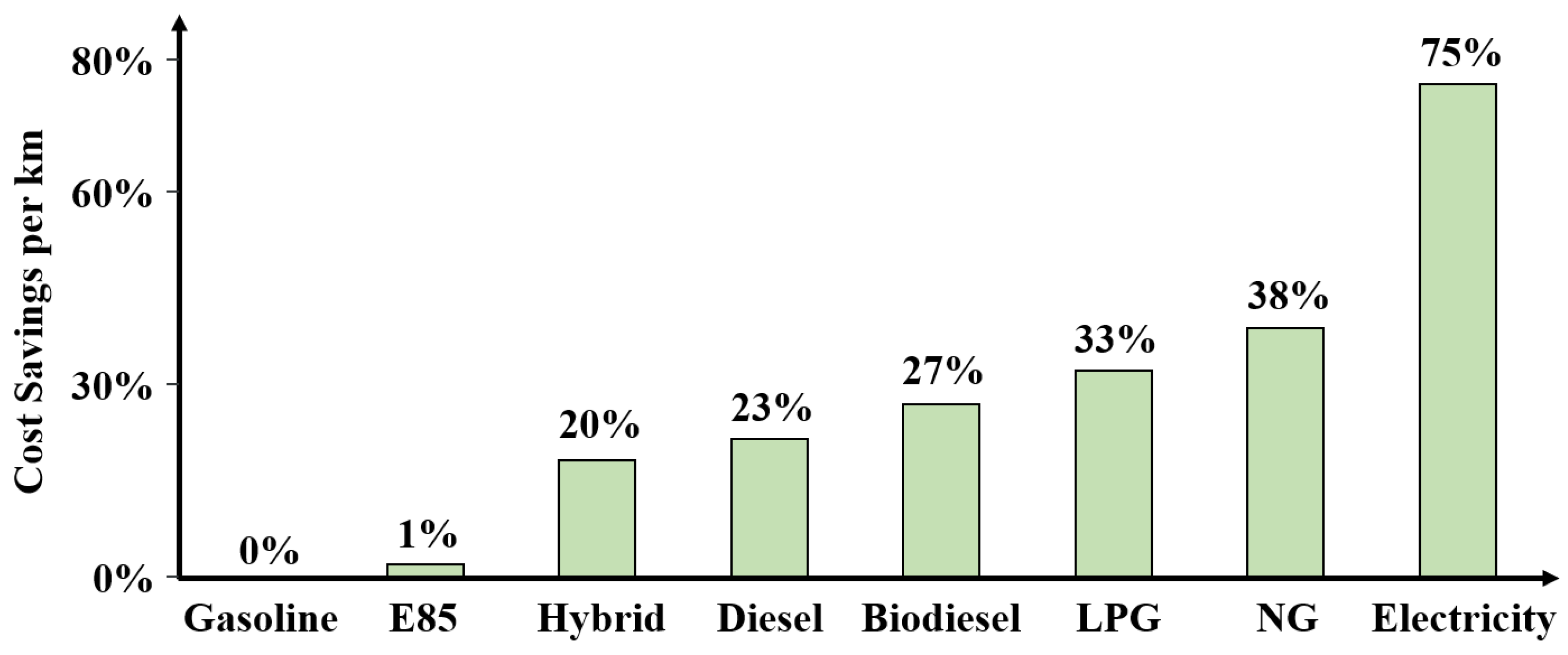
Recently, climate change and carbon neutrality (net-zero) have emerged as major global policy goals. Consequently, the automotive industry is rapidly shifting from internal combustion engine vehicles to eco-friendly electric vehicles. Governments worldwide are strengthening environmental regulations to reduce greenhouse gas emissions and improve energy efficiency. As a result, vehicle powertrains are rapidly shifting from conventional internal combustion engines to electric powertrains, plug-in hybrid systems, and hydrogen fuel cell systems [1,2,3,4,5]. This transition is further accelerated by advances in electrification technologies and growing demand for improved energy efficiency. Global automakers are increasing their research, development, and production investments in electric vehicles to improve their competitiveness in the automotive market. Figure 1 compares the fuel cost savings per driving distance for vehicles using different fuels with those of gasoline vehicles [6]. The results indicate fuel cost savings of approximately 1% for E85 (85% ethanol and 15% gasoline), 20% for hybrid vehicles, 23% for diesel vehicles, 27% for biodiesel vehicles, 33% for LPG vehicles, and 38% for natural gas vehicles. In contrast, electric vehicles achieve a fuel cost reduction of approximately 75%, indicating the highest economic efficiency compared with conventional internal combustion engine vehicles. This economic advantage is due to the lower cost of electricity compared with fossil fuels and the higher energy-conversion efficiency of electric motors compared with internal combustion engines. In addition, regenerative braking recovers kinetic energy during deceleration and reuses some of this energy, thereby further reducing vehicle operating costs. These energy efficiency and economic benefits are key factors driving the adoption of electric vehicles. Accordingly, many countries are promoting vehicle electrification as part of their carbon-neutrality policies. The European Union (EU) and other major countries have introduced policies to restrict or ban the sale of new internal combustion engine vehicles after 2035. In response, global automakers are strengthening their electrification strategies, with a particular focus on electric vehicles. As the electric vehicle market continues to expand, improving the performance and efficiency of traction motors has become increasingly important for extending driving range and enhancing vehicle performance. Electric motors require high power and efficiency. Therefore, motor design and thermal management are important for improving the performance and reliability of electric vehicles, and considerable research has been conducted in these areas.

Figure 1. Comparison of savings in cost per kilometer offered by vehicles powered by gasoline, ethanol(E85), hybrid, diesel, biodiesel, LPG, NGV, and electricity, based on 2010 data [7].

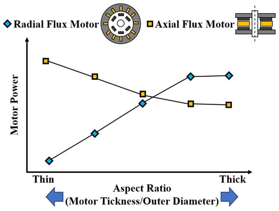
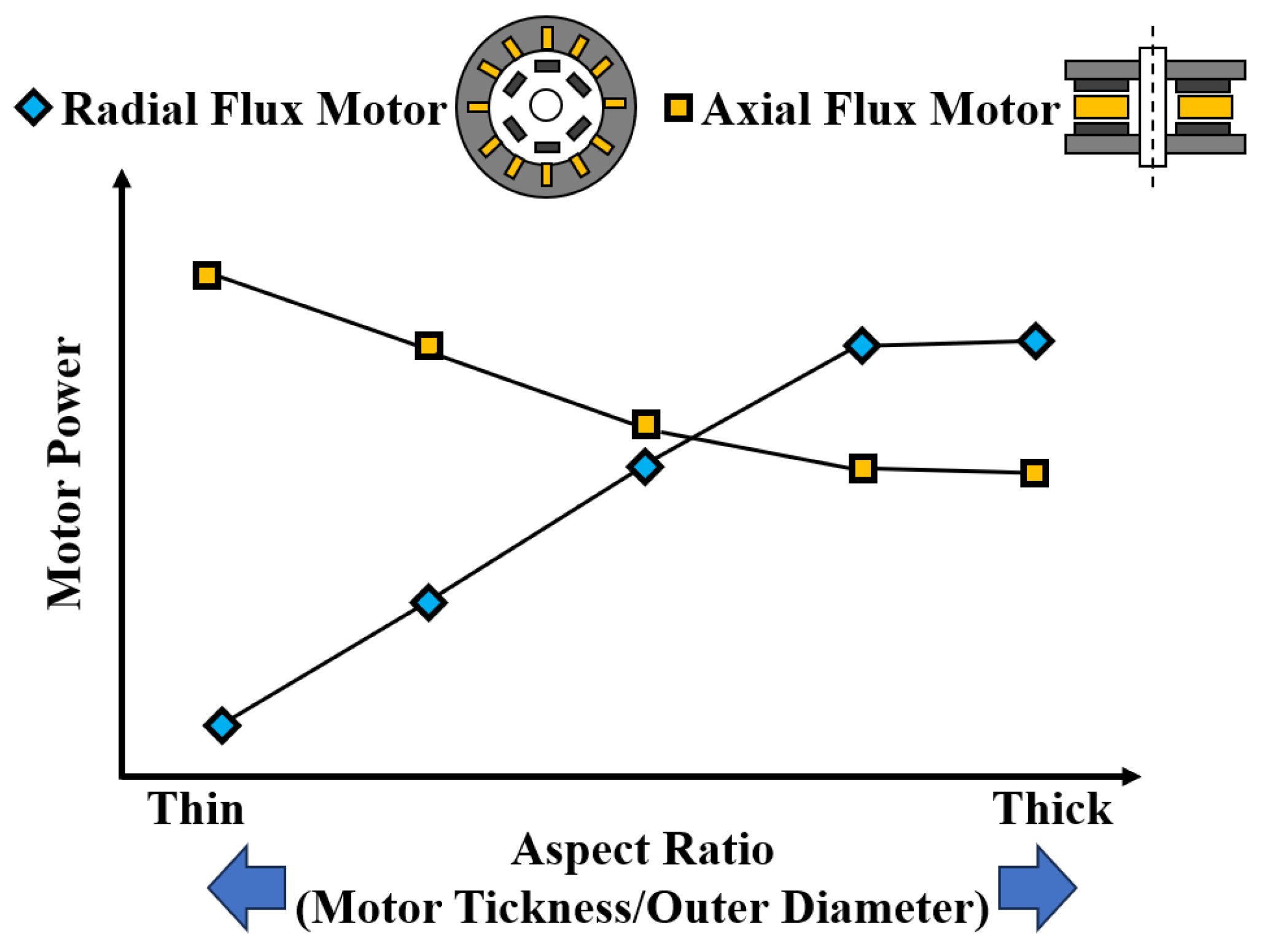
In an electrified powertrain, the traction motor converts electrical energy supplied by the battery and inverter into mechanical energy. The motor plays an important role in determining a vehicle’s driving range, acceleration, and power performance. Therefore, higher motor efficiency can increase the driving range for the same battery capacity. The development of traction motors that provide both high power and high efficiency is thus a key challenge in electric vehicle technology. To meet these requirements, axial-flux motors (AFMs) have received significant attention as next-generation traction motors that can potentially replace conventional radial flux motors (RFMs) [8,9,10,11,12]. Figure 2 compares the output characteristics of RFMs and AFMs as a function of the ratio of motor thickness to outer diameter. In general, as the Aspect Ratio (AR) of RFMs decreases, their axial length decreases, leading to a reduction in the effective air-gap area. Consequently, the output performance gradually deteriorates. In contrast, under the same conditions, AFMs showed an increase in output power as the AR decreased. This behavior is attributed to its disk-shaped structure. As the outer diameter increases, the effective area available for magnetic flux increases, resulting in better magnetic flux utilization. Because of these structural characteristics, AFMs can achieve high torque and power densities. Their thin disk-shaped structure also makes them suitable for space-constrained applications, such as vehicle underbodies and in-wheel systems. Therefore, AFMs are considered promising traction motors for next-generation electric vehicles because they can provide high power while maintaining a compact and lightweight structure.

Figure 2. Schematic representation of the effect of aspect ratio on the output power characteristics of radial and axial-flux motors [13,14].

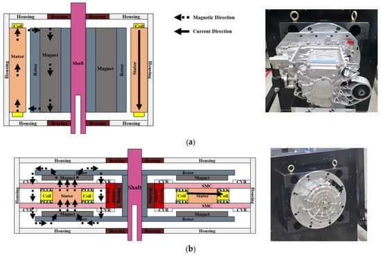
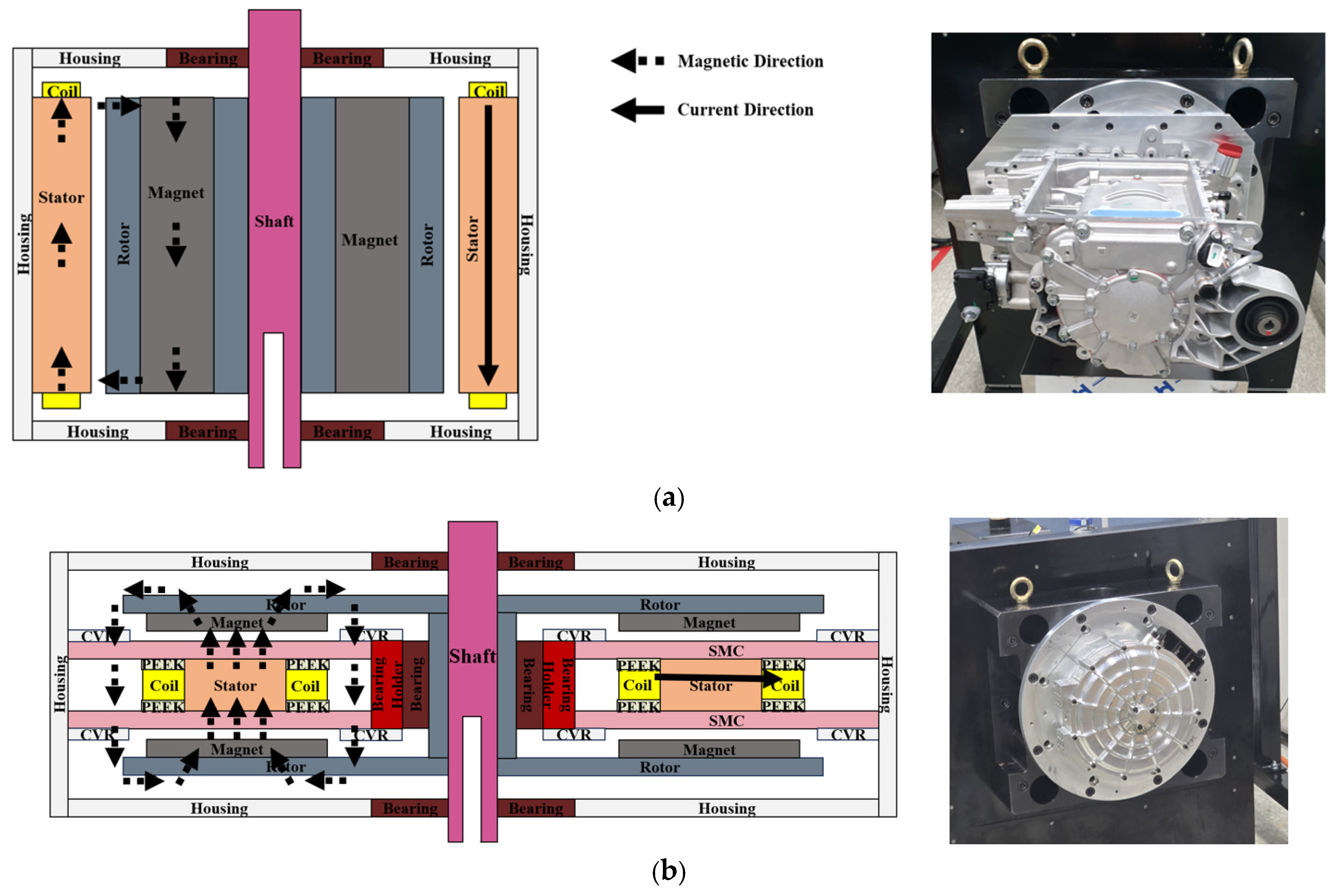
Figure 3 compares the structural characteristics and magnetic flux directions of RFMs and AFMs. As shown in Figure 3a, in RFMs, current flows through the coils and generates magnetic flux in the radial direction. This magnetic flux interacts with the permanent magnets on the rotor to produce torque. However, the magnetic flux follows a relatively long radial path, along which flux leakage can occur. Therefore, magnetic flux utilization may be relatively low [15,16]. In contrast, as shown in Figure 3b, AFMs guide magnetic flux along a short axial path, resulting in low magnetic reluctance and high flux-transfer efficiency. In addition, their disk-shaped structure provides a large effective area for magnetic flux. Consequently, AFMs can achieve high magnetic flux density and torque density within the same volume [17,18]. Owing to these structural characteristics, AFMs have attracted significant attention as next-generation traction motors for electric vehicles because they can achieve both high power and high efficiency.

Figure 3. Schematic diagram of axial and radial flux motor structures: (a) RFMs, (b) AFMs.

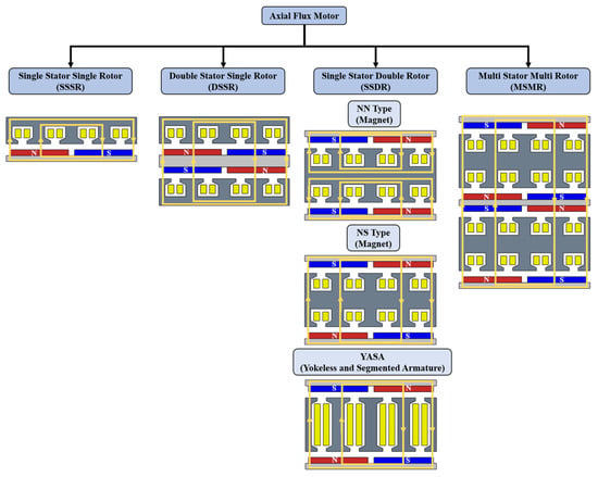
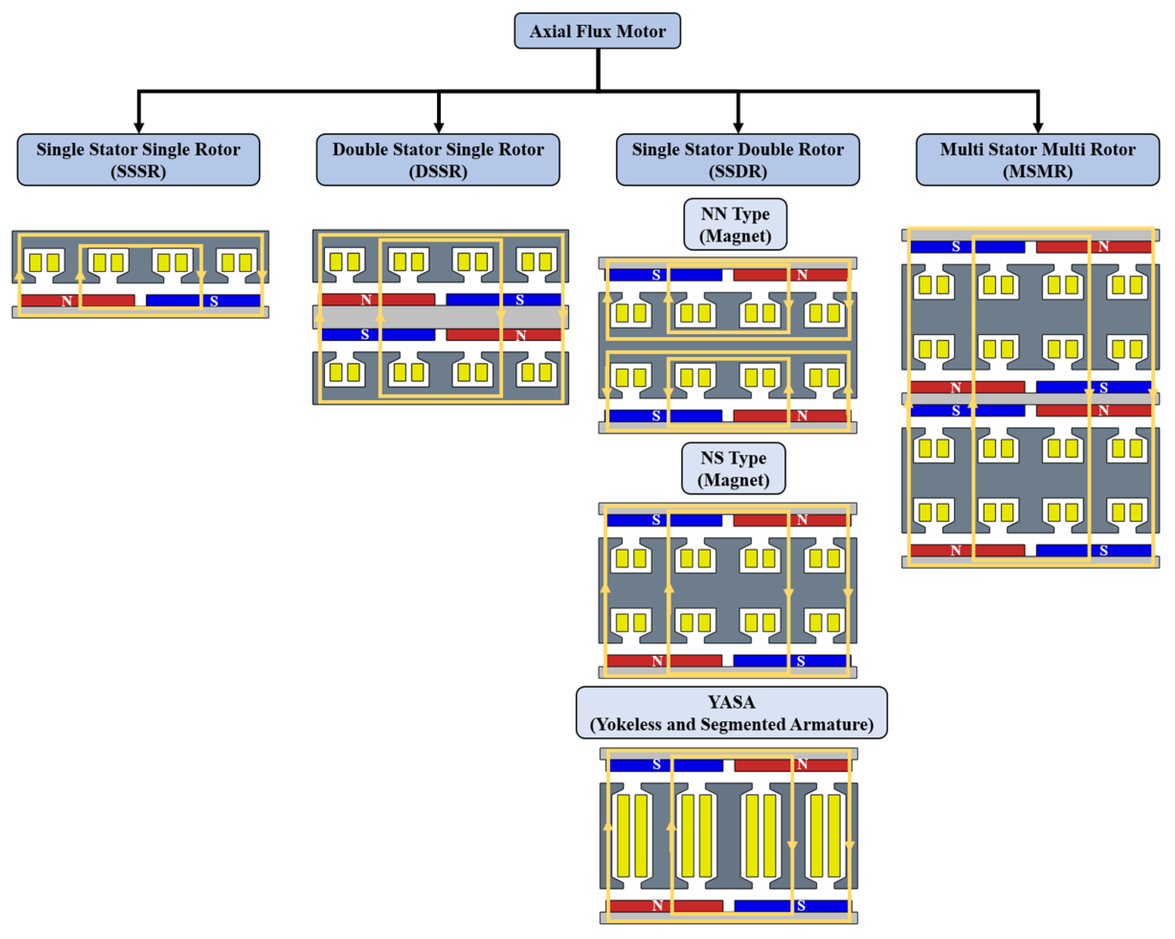
AFMs can be classified into various structures according to the arrangement of the stators and rotors. Figure 4 shows typical AFM structures. AFMs can be classified into four types: single-stator single-rotor (SSSR), double-stator single-rotor (DSSR), single-stator double-rotor (SSDR), and multi-stator multi-rotor (MSMR) [19]. The SSSR is the most basic structure. The DSSR and SSDR use double-stator and double-rotor structures, respectively, to improve magnetic flux utilization and torque density. The MSMR consists of multiple stators and rotors stacked together, making it suitable for high-power motor applications. In addition, the Yokeless and Segmented Armature (YASA) structure eliminates the stator yoke and uses segmented coils. This structure reduces iron loss and weight while maintaining high torque density, making it suitable for electric vehicle traction motors.

Figure 4. Structural classification of AFMs. The yellow arrows indicate the magnetic flux directions.

Therefore, AFMs offer high power and torque densities. However, their high power density can result in more losses within the same volume, necessitating effective thermal management. Accordingly, many studies have investigated various cooling technologies and multiphysics analysis methods to improve the thermal performance of AFMs. Shen et al. [20] suggested the need for an efficient cooling system to manage the increased thermal load caused by the high power density of AFMs. Chen et al. [21] proposed a spiral cooling channel using nanofluids that demonstrated better heat-transfer performance than a conventional structure. Gao et al. [22] compared different water-cooling channel structures for AFMs and demonstrated improvements in cooling performance and energy efficiency. Zhao et al. [23] applied a hybrid cooling system combining rotor oil spray cooling with stator spiral water-channel cooling. The proposed system improved thermal management performance, and its reliability was verified through prototype testing. Qiao et al. [24] combined electromagnetic loss analysis with computational fluid dynamics (CFD)-based thermal fluid analysis and achieved high accuracy in temperature prediction. Su et al. [25] proposed an analysis method that combines electromagnetic analysis with a lumped-parameter thermal network(LPTN). This method significantly reduces computational time while showing good agreement with the experimental results. Recently, Qiu et al. [26] applied a honeycomb-shaped cooling oil groove to effectively reduce the maximum temperatures of the coil and stator. Jenkins et al. [27] analyzed various thermal management methods for AFMs, including air, water, oil, immersion, and heat-pipe cooling. They also proposed effective cooling strategies for high-power-density traction motors. These studies demonstrate that various cooling structures and analysis methods can improve the thermal performance of AFMs. However, most previous studies have focused on optimizing cooling structures or thermal performance under a single operating condition. In this study, the losses calculated from electromagnetic analysis were applied as heat sources in three-dimensional CFD-based thermal-fluid analysis. The cooling performance and temperature distribution of the AFM were then analyzed. This study aimed to investigate the relationship between electromagnetic losses and thermal-fluid characteristics and to provide design guidelines for improving the thermal management performance of the AFM.

2. Electromagnetic Field Analysis

The motor converts electrical energy into mechanical rotational energy, during which various types of losses occur. These losses are converted into heat, increasing the temperature inside the motor and directly affecting its efficiency and durability. In general, motor losses are classified into copper, iron, and mechanical losses. The total motor loss is expressed by Equation (1), where P_total is the total loss, P_cu is the copper loss, P_iron is the iron loss, and P_mech is the mechanical loss. Because this study focuses on the electromagnetic characteristics of the motor, mechanical losses caused by bearing friction and air resistance were assumed to be relatively small and were therefore neglected.

P_total ≈ P_cu + P_iron

(1)

Copper loss accounts for the largest portion of the total motor loss. YASA motors are generally affected by AC copper losses owing to factors such as inverter switching frequency, magnetic flux leakage in the stator slots, skin effect, and proximity effect. When current flows through the coils, Joule loss is generated because of the electrical resistance of the conductor. Therefore, the heat generated in the coils increases with the square of the current. In general, AFMs operate at relatively low speeds; therefore, the effect of high-frequency magnetic fields on copper loss is relatively small. When the current frequency is below 1 kHz, the losses due to the skin and proximity effects can therefore be neglected. The copper losses are expressed by Equations (2)–(5), and the definitions and units of the symbols used in these equations are summarized in Table 1. The copper loss in the AFM can be expressed by Equation (5) by substituting Equations (3) and (4) into Equation (2).

$${\mathrm{P}}_{\mathrm{cu}}=\mathrm{m}{\mathrm{I}}_{\mathrm{rms}}^2{\mathrm{R}}_{\mathrm{AC}}$$

(2)

m_cu = ρNl_avgS_c

(3)

$${\mathrm{R}}_{\mathrm{AC}}={\mathrm{k}}_{\mathrm{R}}·{\displaystyle \frac{\mathrm{N}{\mathrm{l}}_{\mathrm{avg}}}{\mathsf{\sigma }{\mathrm{S}}_{\mathrm{c}}}}$$

(4)

$${\mathrm{P}}_{\mathrm{cu}}=\mathrm{m}{\mathrm{I}}_{\mathrm{rms}}^2{\displaystyle \frac{{\mathrm{k}}_{\mathrm{R}}{\mathrm{m}}_{\mathrm{cu}}}{\mathsf{\sigma }\mathsf{\rho }{\mathrm{S}}_{\mathrm{c}}^2}}=\mathrm{m}{\mathrm{J}}^2{\displaystyle \frac{{\mathrm{k}}_{\mathrm{R}}{\mathrm{m}}_{\mathrm{cu}}}{\mathsf{\sigma }\mathsf{\rho }}}$$

(5)

Table 1. Definition of symbols used in Equations (2)–(5).

Symbol	Definition	Unit
Pcu	Copper loss	W
m	Number of phases	-
Irms	RMS Phase current	A
RAC	AC resistance	Ω
mcu	Copper mass	kg
ρ	Copper density	kg/m3
N	Number of coil turns	-
lavg	Average length per turn	m
σ	Electrical conductivity of the conductor	S/m
SC	Cross-sectional area of the conductor	m2
kR	Coefficient of resistivity	-
J	Current density of the conductor	A/m2

Iron loss occurs in magnetic core materials, such as the stator and rotor, due to changes in the alternating magnetic field. It consists primarily of hysteresis and eddy-current losses. Iron loss is affected by factors such as magnetic flux density, frequency, stacking factor, and manufacturing processes. The iron loss P_iron is expressed by Equation (6), where K_h is the Hysteresis loss coefficient determined from the B-H curve of the magnetic material. f is the frequency, B is the magnetic flux density, and Y is the empirical coefficient depending on the material properties and generally ranges from 1.6 to 2.2. K_c is the eddy current loss coefficient, and K_e is a coefficient used to account for additional nonlinear losses.

When an electrical conductor, such as a permanent magnet, iron core, or busbar, is exposed to a magnetic field, an induced current is generated inside the conductor. This current produces Joule heating due to the electrical resistance of the conductor, resulting in eddy current loss.

P_iron = K_hfB^Y + K_c(fB)² + K_e(fB)^1.5

(6)

The commercial software used in this study was applied to Equation (7) to account for eddy current effects. Here, σ is the electrical conductivity, j is the imaginary unit, ω is the angular frequency, ϵ is the permittivity, and ∇ is the spatial differential operator. H is the magnetic field intensity, μ₀ is the vacuum permeability, and μ_r is the relative permeability.

$${\mathrm{P}}_{\mathrm{iron},\mathrm{eddy}}=\nabla \times \left({\displaystyle \frac{1}{\mathsf{\sigma }+\mathrm{j}\mathsf{\omega }\mathsf{ϵ}}}·\left(\nabla \times \mathrm{H}\right)\right)=\mathrm{j}\mathsf{\omega }{\mathsf{\mu }}_0{\mathsf{\mu }}_{\mathrm{r}}\mathrm{H}$$

(7)

2.1. 3D Modeling

In this study, a commercially available motor (P model) developed by Company Y, a motor manufacturer based in the United Kingdom (UK), with a rated output power of 160 kW, was used as a reference for the electromagnetic analysis of an AFM for electric vehicles. Based on the publicly available specifications and structural characteristics of this motor, a base model was independently designed by the authors for electromagnetic performance evaluation and subsequent thermal management optimization.

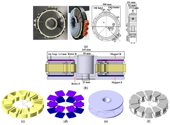
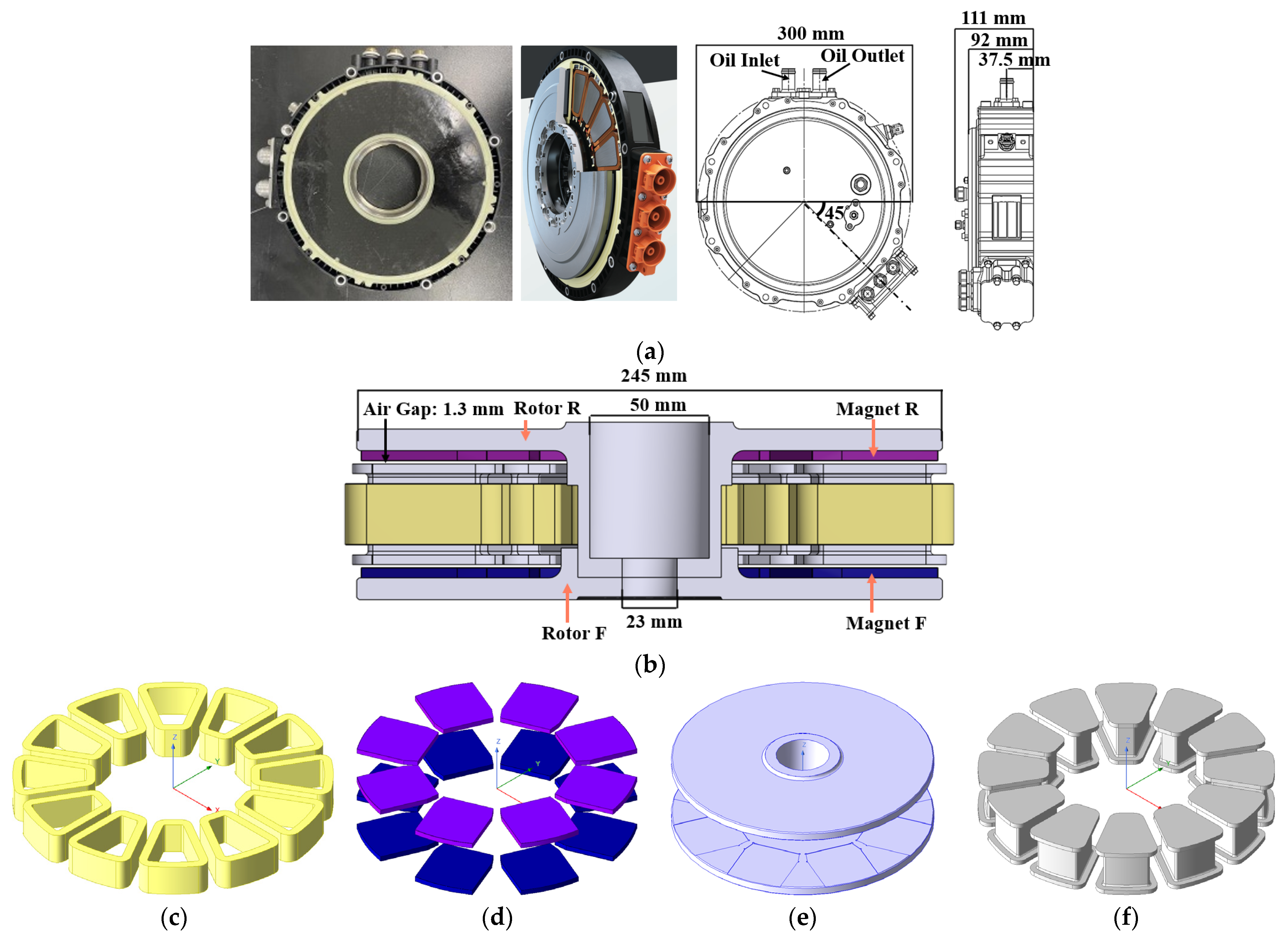
Figure 5 compares the structures of (a) the benchmark motor and (b) the base model designed in this study. Similar to the Company Y model, the base model adopts an SSDR structure with 12 slots and 8 poles. Based on the benchmark motor, an electromagnetic analysis model was designed considering the main geometric specifications, including the rotor diameter, air gap, and the number of coils and permanent magnets. Figure 5c–f show the main components of the analysis model: (c) coil, (d) permanent magnets, (e) rotor, and (f) stator. The primary specifications of the analysis model are listed in Table 2. The motor adopts an axial flux structure with 12 slots and 8 poles. No skew was applied to the permanent magnets, and the coils were designed with 16 turns.

Figure 5. AFM benchmarking and base model structure: (a) benchmark model, (b) base model, (c) coil, (d) magnet, (e) rotor, (f) stator.

Table 2. Specification of AFM.

Specification		Unit	Value
Motor type		-	AFM/SSDR
Number of pole/slot		-	8 pole/12 slot
Length of air gap		mm	1.3
Stator	Diameter of outer/inner	mm	125/65
	Thickness	mm	42
Rotor	Diameter of outer/inner	mm	122.5/25
	Thickness	mm	9
Magnet	Skew angle	Deg.	-
	Width	mm	53.5
	Thickness	mm	4.8
	Diameter of outer/inner	mm	122.5/64
Coil	Number of turns per coil	Turn	16
	Diameter (width/height)	mm	7/1.6

2.2. Boundary Conditions and Properties

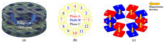
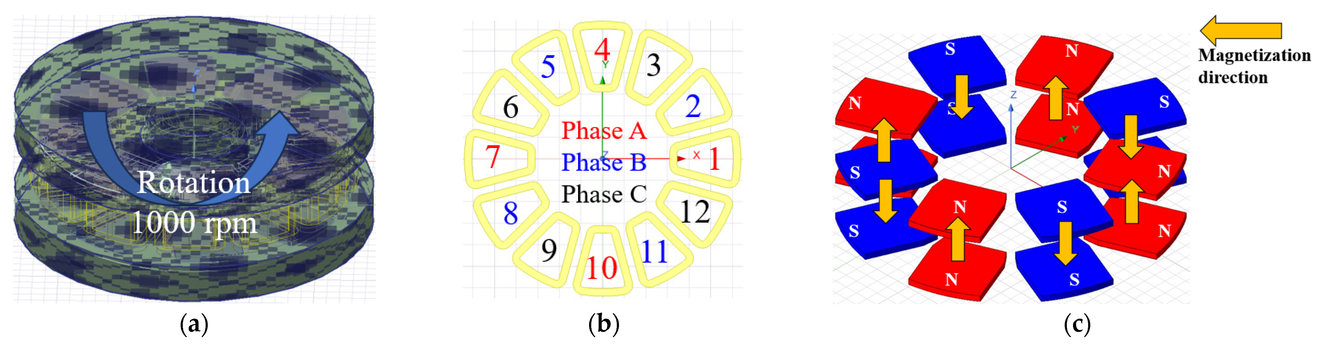
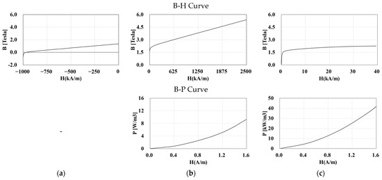
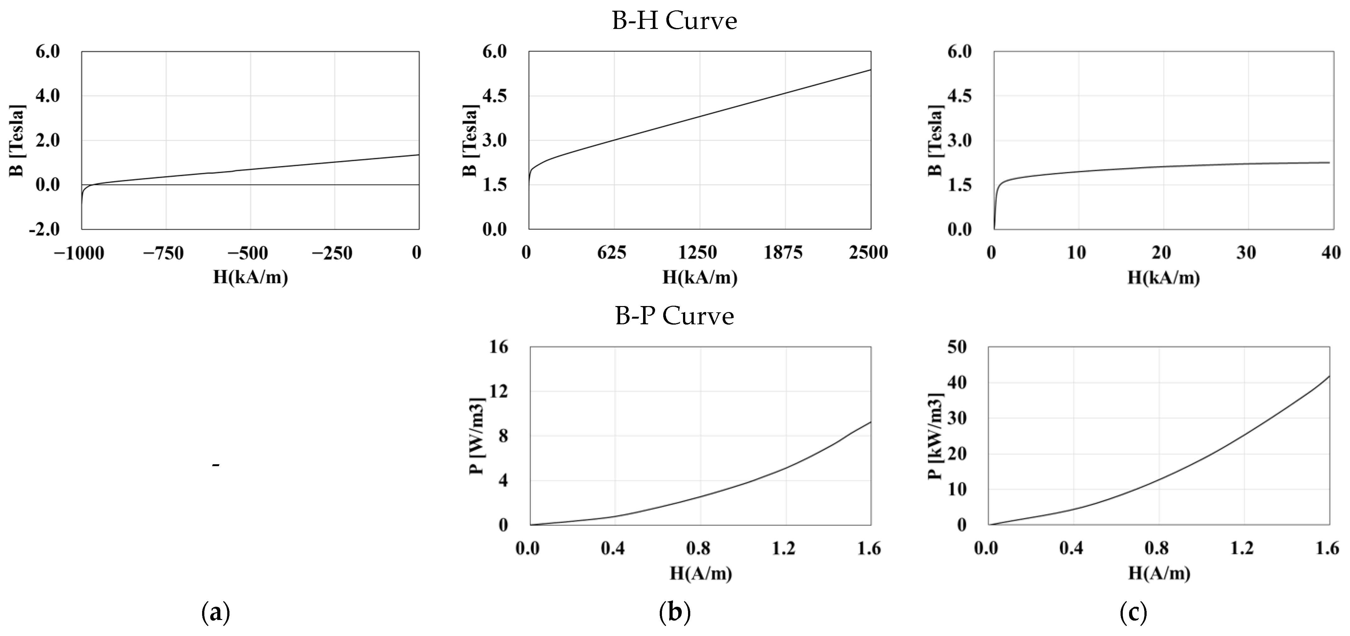
Commercial software (ANSYS Maxwell 2025R1) was used to perform the electromagnetic analysis of the motor. Figure 6 shows the electromagnetic analysis conditions. The motor was set to rotate counterclockwise at 1000 rpm, with the shaft, rotors, and permanent magnets defined as the rotating components(Figure 6a), and the coils were configured with a Y-connection. The coils were assigned to the phases according to their positions as follows: phase A (1, 4, 7, and 10), phase B (2, 5, 8, and 11), and phase C (3, 6, 9, and 12), as shown in Figure 6b. Electrical insulation was also applied to prevent current leakage from the coils. The permanent magnets were arranged with alternating N and S poles, with the magnetization directions defined as +Z for the N poles and −Z for the S poles, as shown in Figure 6c. The materials and properties of each component are listed in Table 3 and illustrated in Figure 7.

Figure 6. Boundary conditions and settings: (a) rotational condition, (b) phase coil assignment, (c) magnetization direction setting.

Table 3. Properties of AFM.

Part	Coil	Magnet	Rotor	Stator
Material	Copper	NdFeB (N45)	50PN800	Vacoflux 17
Relative permeability [-]	0.9999	B-H curve	B-H curve	B-H curve
Bulk conductivity [Siemens/m]	58,000,000	15,000	4,166,670	2,439,024
Magnetic coercivity [A/m]	0	−905,300	0	0
Core loss model [W/m3]	None	None	B-P curve	B-P curve

Figure 7. B-H and B-P curves for individual parts: (a) magnet, (b) rotor, (c) stator.

2.3. Calculation Grid and Analysis Setting

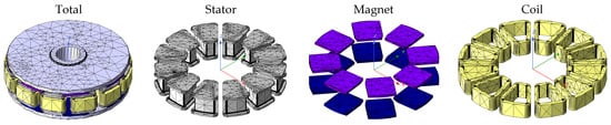
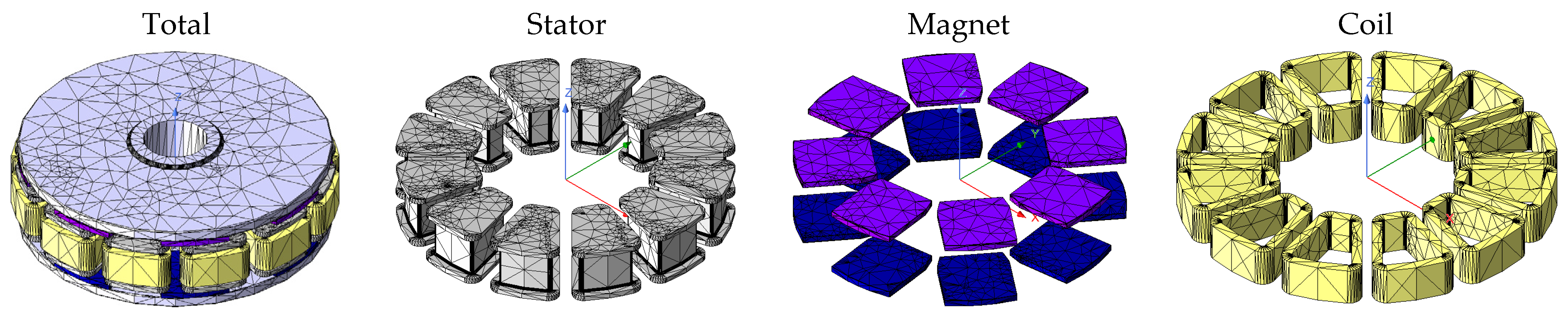
A tetrahedral mesh was generated for the computational domain. The mesh size was adjusted according to the geometry and size of each component. To improve the mesh resolution in critical regions, the length-based mesh refinement function in ANSYS Maxwell was applied, with a maximum element length of 2 mm. This refinement was applied to the major electromagnetic components to more accurately resolve the electromagnetic field distribution. The generated mesh model is illustrated in Figure 8. Approximately 333,000 computational cells were used in the analysis. The back-EMF analysis was performed under open-circuit conditions at 1000 rpm. A time step of 0.000041666 s and a total analysis time of 0.015 s were used, with the total analysis time corresponding to one electrical cycle (360°).

Figure 8. Computational mesh for each part.

2.4. Cogging Torque

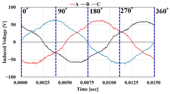
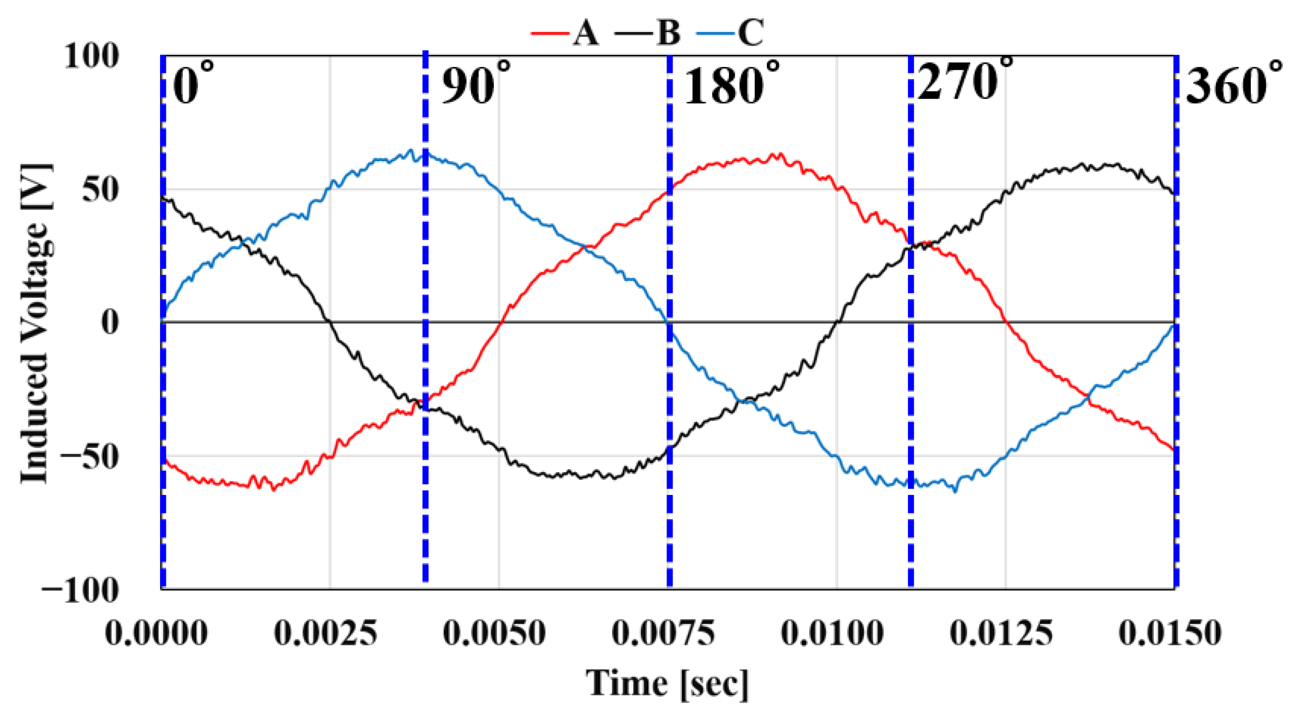
The back EMF was calculated under open-circuit conditions. The coil terminals were defined as open circuits, and no external current excitation was applied; therefore, the phase current was 0 A. The rotor was rotated at 1000 rpm, and the voltage induced in each phase coil by the time-varying magnetic flux of the permanent magnets was calculated as the back EMF. A high load resistance was not used because the open-circuit condition was directly applied to the coil terminals. Figure 9 shows the calculated back EMF. Sinusoidal induced voltages were generated in the coils as the electrical angle of the AFM changed. The three phases (A, B, and C) exhibited phase differences of 120°. The voltage waveforms were symmetrically distributed over a range of approximately ±60 V. These results indicate that the motor exhibits electromagnetic symmetry and generates a balanced three-phase voltage.

Figure 9. Induced voltage graph (@1000 rpm).

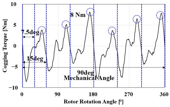
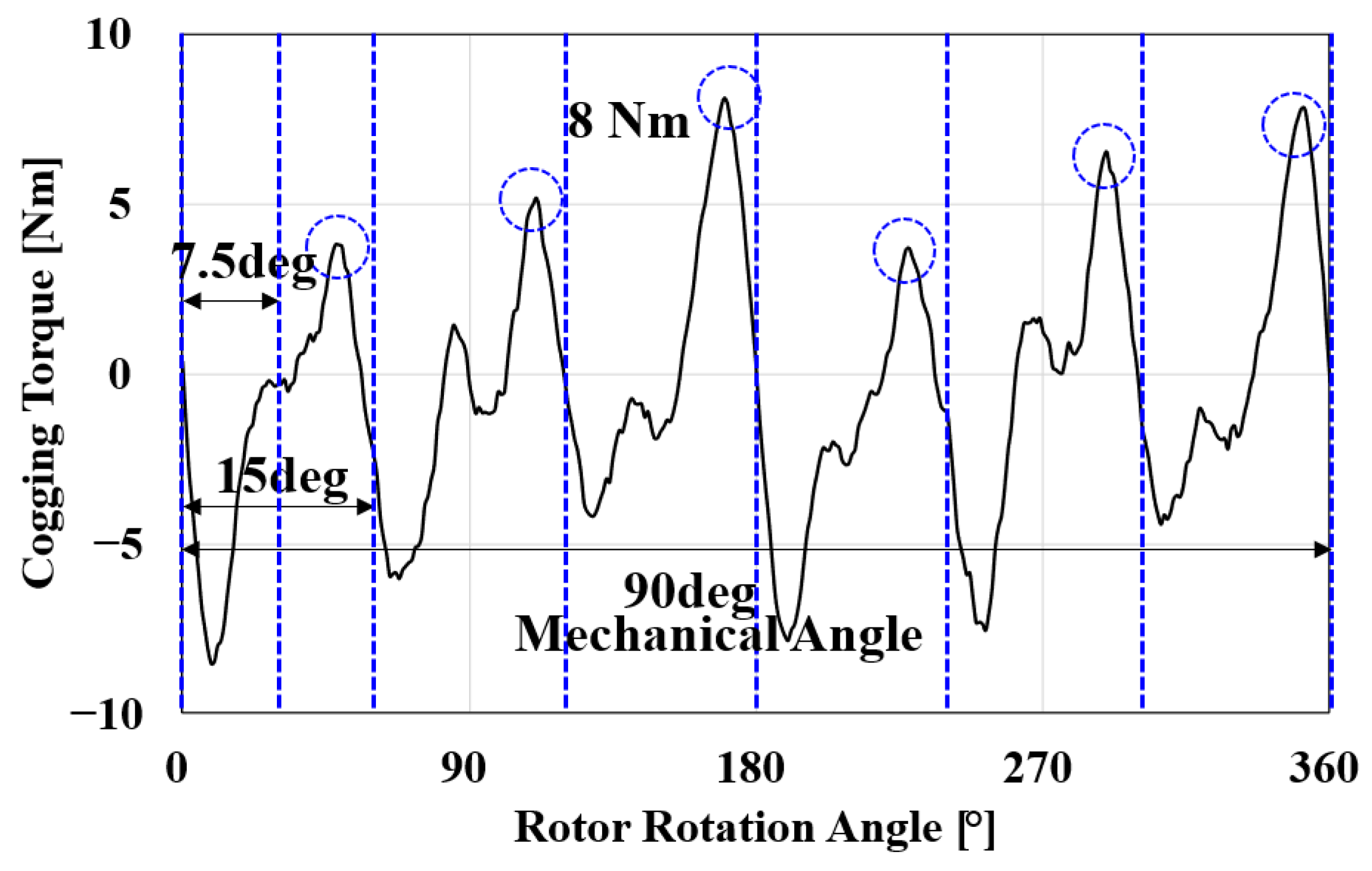
Figure 10 shows the cogging torque of the base model. Cogging torque is a periodic torque variation caused by the magnetic interaction between the rotor and stator. It is an important factor affecting the rotational smoothness, vibration, and noise of the motor. As shown in Figure 10, 12 periodic torque fluctuations occur during one mechanical period of 90°. This behavior results from the interaction between the rotor and the 12 stator slots during rotation. The maximum absolute value of the cogging torque waveform was approximately 8 N·m. For comparison with the shaft torque, an operating condition of 1000 rpm and 300 A was used. The average shaft torque at this operating point was 313 N·m, and the maximum cogging torque corresponded to approximately 2.6% of the average shaft torque. The basic period of the cogging torque was approximately 7.5° in mechanical angle, corresponding to the stator slot pitch. These periodic torque fluctuations can cause rotational instability, vibration, and noise, particularly at low speeds. Therefore, cogging torque should be reduced through measures such as slot skew or magnet shape optimization.

Figure 10. Cogging torque graph (@1000 rpm).

2.5. Power and Efficiency

Based on the back-EMF analysis results, current was applied to calculate the motor efficiency and output power. All results presented in this section were obtained from electromagnetic simulations. The motor has three phases, with a phase difference (θ) of 120° between phases A, B, and C. Based on Equation (8), the three-phase sinusoidal currents were applied to Phases C, A, and B sequentially, with a phase displacement of 120° between each phase. The input current of the electric motor is an alternating current that changes with time, directly affecting the rotor magnetic flux and torque generation. Table 3 lists the analysis conditions used to calculate the torque and motor efficiency. Eighteen cases were analyzed to evaluate motor performance under different operating conditions. Each case was defined by a different combination of rotational speed and input current to evaluate their effects on torque and efficiency. The time step and stop time were adjusted according to the rotational speed, and the values applied to each operating condition are listed in Table 4.

Phase Input current = I_peak + sin(ωt − θ)

(8)

Table 4. Input current conditions for each model.

No.	Irms [A]	Ipeak [A]	ω [rpm]	fe [Hz]	fm [Hz]	Time Step [s]	Stop Time [s]
1	450	636.39	1000	66.66	16.66	0.000041666	0.0150
2			2000	133.33	33.33	0.000020833	0.0075
3			3500	233.33	58.33	0.000011905	0.0043
4			4130	275.33	68.83	0.000010088	0.0036
5			5000	333.33	83.33	0.000008333	0.0030
6			6000	400.00	100.00	0.000006944	0.0025
7	300	424.26	1000	66.66	16.66	0.000041666	0.0150
8			3500	233.33	58.33	0.000011905	0.0043
9			4000	266.67	66.67	0.000010417	0.0038
10			4500	300.00	75.00	0.000009259	0.0033
11			5000	333.33	83.33	0.000008333	0.0030
12			6000	400.00	100.00	0.000006944	0.0025
13	225	318.20	1000	66.66	16.66	0.000041666	0.0150
14			3500	233.33	58.33	0.000011905	0.0043
15			5000	333.33	83.33	0.000008333	0.0030
16	150	212.13	1000	66.66	16.66	0.000041666	0.0150
17			3500	233.33	58.33	0.000011905	0.0043
18			5000	333.33	83.33	0.000008333	0.0030

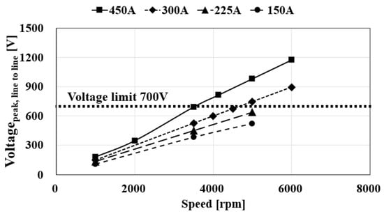
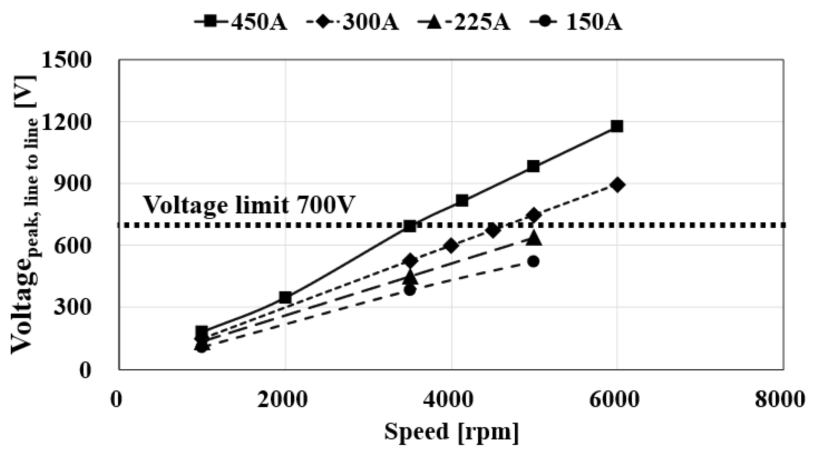
In this study, an 800 V battery pack was used for the drive system, and the inverter employed the space-vector pulse-width modulation (SVPWM) method. The maximum line-to-line voltage generated by the SVPWM controller is limited to approximately 86.6% of the DC-link voltage owing to the characteristics of the active voltage vectors. Therefore, for a DC voltage of 800 V, the maximum line-to-line voltage is approximately 700 V. Figure 11 shows the maximum line-to-line voltages for the 18 analyzed cases. The line-to-line voltage increased with rotational speed under all current conditions because the back EMF increases with speed as the magnetic flux varies more rapidly. Considering the 700 V voltage limit, the line-to-line voltage exceeded this limit at 3500 rpm at 450 A, 4500 rpm at 300 A, 5480 rpm at 225 A, and 7260 rpm at 150 A.

Figure 11. Line-to-line voltage comparison graph according to rotation speed (at ϕ = 0).

At high speeds, the back EMF of the motor increases rapidly. When the required line-to-line voltage exceeds the inverter voltage limit, the motor enters the voltage-limited operating region, resulting in reduced torque capability. As the rotational speed increases, a higher voltage is required to overcome the increasing back EMF. To mitigate this voltage limitation, a current phase angle shift technique was applied. This technique emulates the principle of flux-weakening control commonly implemented in field-oriented control (FOC), in which the d-axis and q-axis current components are adjusted to reduce the effective magnetic flux linkage and satisfy the inverter voltage constraint. In this study, the current phase angle was directly adjusted in the electromagnetic analysis without implementing a closed-loop control algorithm. By modifying the current phase angle, the required terminal voltage can be reduced, thereby extending the operating speed range of the motor. Current phase angles were applied to five cases (Cases 4–6, 11, and 12) that exceeded the line-to-line voltage limit. The applied current phase angles are listed in Table 5. Further analyses were conducted by applying different phase angles to Equation (9) for each case.

$$\mathrm{Input} \mathrm{current}={\mathrm{I}}_{\mathrm{peak}}+\sin \left(\mathsf{\omega }\mathrm{t}-\mathsf{\theta }+\left(\mathsf{\varphi }\times {\displaystyle \frac{\mathsf{\pi }}{180}}\right)\right)$$

(9)

Table 5. Input current conditions for each model with current phase-angle adjustment to satisfy the voltage limit.

No.	Irms [A]	Ipeak [A]	ω [rpm]	ϕ [deg]
4	450	636.39	4130	0
				10
				10.5
				11.3
				20
5			5000	0
				20
				28
				30
6			6000	0
				30
				43
				50
11	300	424.26	5000	0
				10
12			6000	0
				15
				20

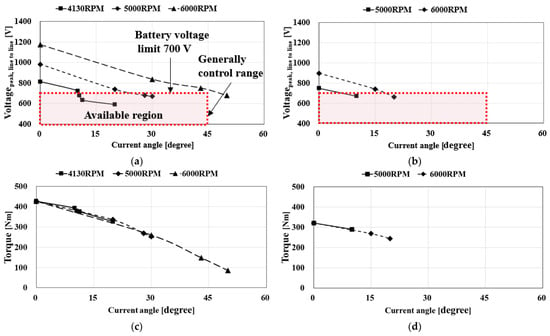
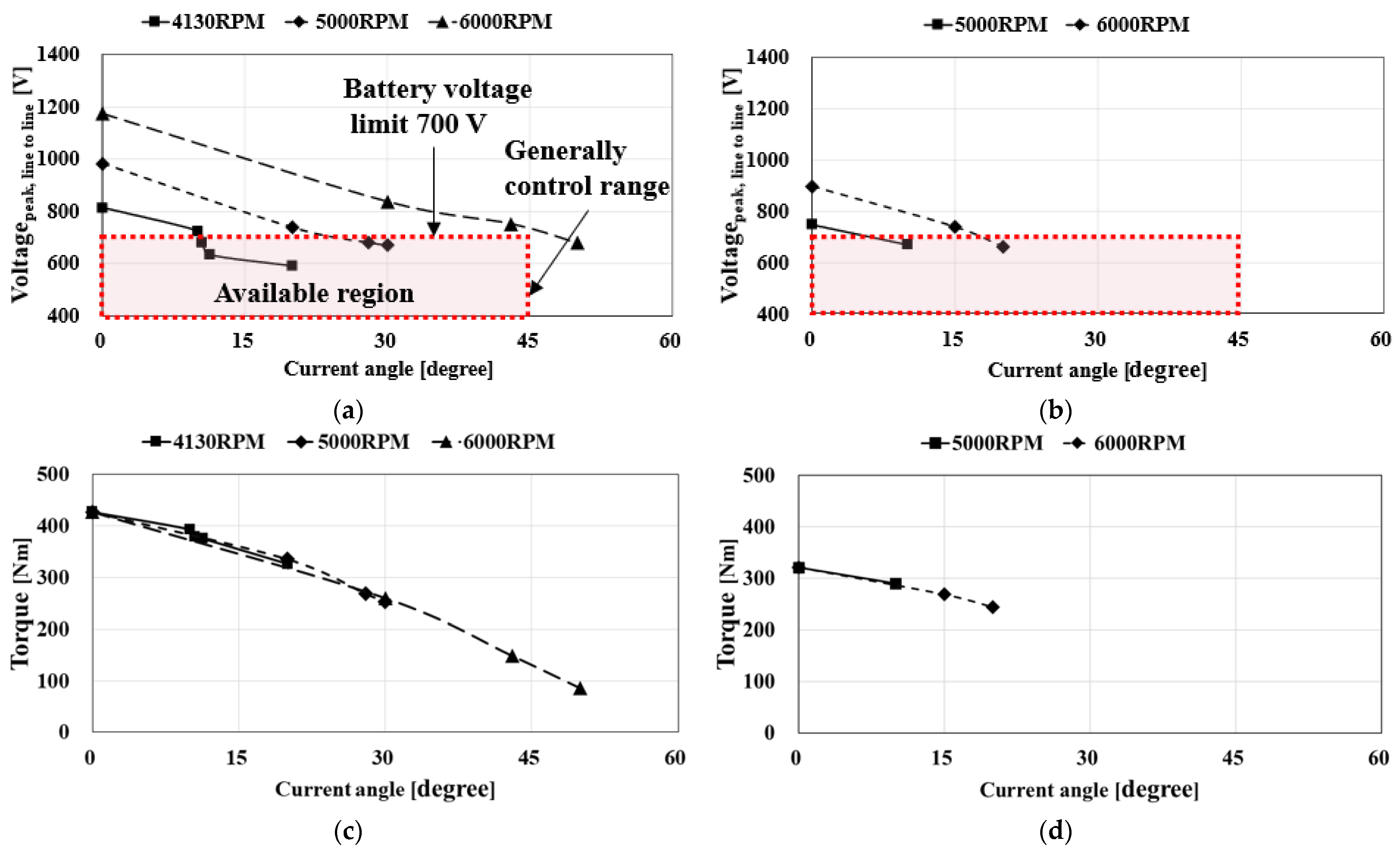
The analysis results for the current phase angles are shown in Figure 12, and the selected operating conditions are summarized in Table 6. As shown in Figure 12a,b, increasing the current phase angle reduced the line-to-line voltage, allowing the 700 V voltage limit to be satisfied at high rotational speeds. Accordingly, the required phase angle increased with rotational speed. Figure 12c,d show that the torque decreased as the current phase angle increased. At 450 A, the torque reduction became particularly significant at high rotational speeds, decreasing from 427 N·m at 0° to 86 N·m at the selected phase angle of 50° at 6000 rpm. A similar trend was observed at 300 A. These results indicate that increasing the current phase angle enables operation within the voltage limit but results in a corresponding reduction in torque, particularly at high rotational speeds. Therefore, the current phase angle should be selected considering both the voltage limit and torque performance.

Figure 12. Effect of current phase angle on line to line voltage and torque: (a) Voltage_{peak, line to line} (450 A), (b) Voltage_{peak, line to line} (300 A), (c) Torque (450 A), (d) Torque (300 A).

Table 6. Selected current phase angles satisfying the voltage limit and corresponding torque characteristics.

Current [A]	Speed [rpm]	Voltage-Limit Current Angle [deg]	Torque at 0° [N·m]	Torque at Voltage Limit [N·m]	Torque Reduction [%]
450	4130	10.5	427	379	11.2
	5000	28	427	269	37.0
	6000	50	427	86	79.9
300	5000	10	322	290	9.9
	6000	20	321	244	24.0

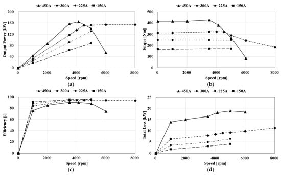
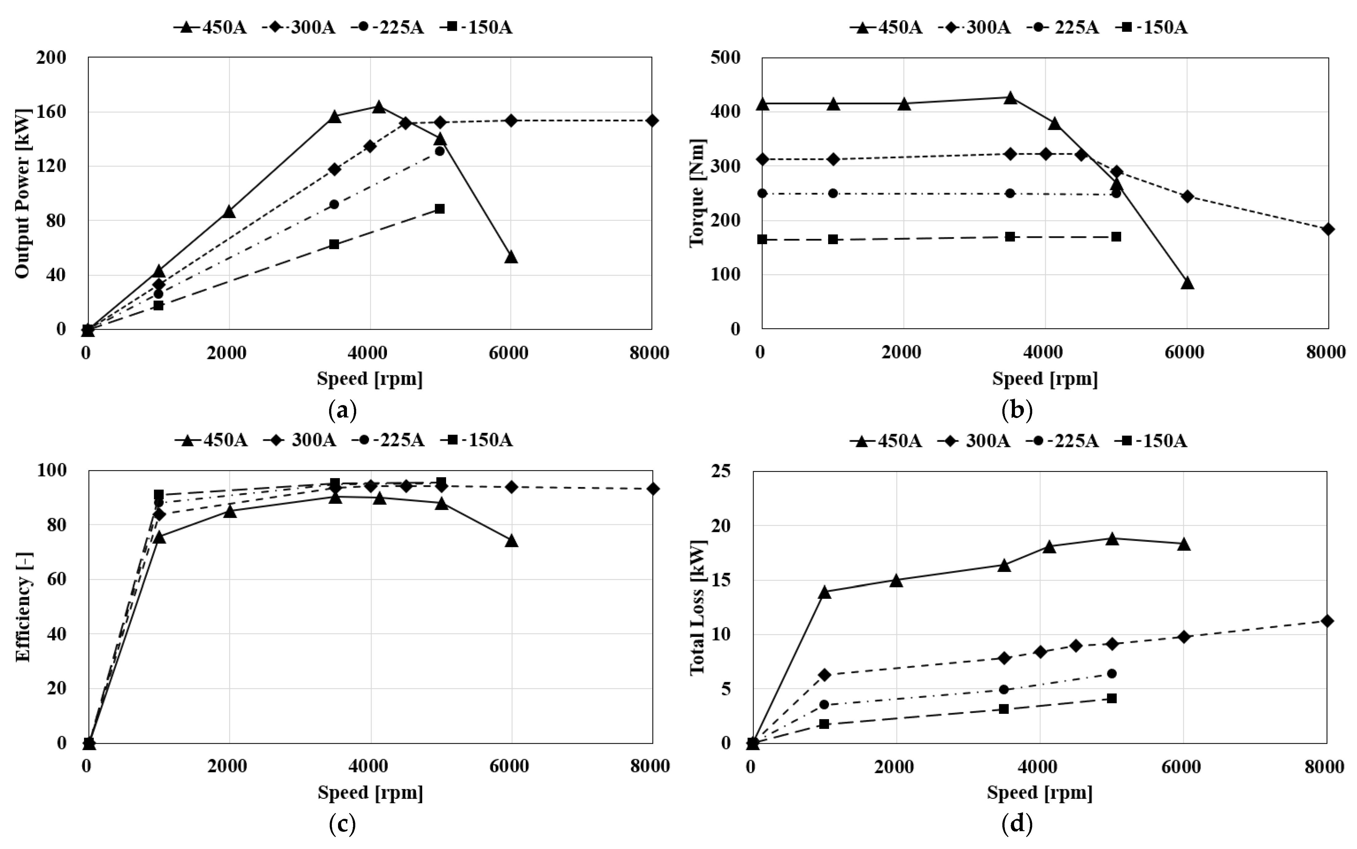
Figure 13 summarizes the analysis results considering the voltage limit, including torque (a), output power (b), efficiency (c), and total loss (d) for different input currents and rotational speeds. Figure 13a compares the torque at different input currents. At 450 A, the torque remained relatively constant at approximately 415 N·m below 4130 rpm but decreased rapidly above this speed. At 6000 rpm, the torque decreased significantly to 86 N·m. This reduction was attributed to the increase in current phase angle with rotational speed, which reduces the magnetic flux in the motor. Therefore, operation above 6000 rpm was considered difficult at 450 A. At 300 A, the torque remained nearly constant at approximately 322 N·m up to 4500 rpm, then gradually decreased to 290 N·m at 5000 rpm and 244 N·m at 6000 rpm. In contrast, at 225 and 150 A, the torque remained nearly constant at approximately 249 and 169 N·m, respectively, up to 5000 rpm. Figure 13b shows the output power at different input currents. At 450 A, the output power increased with rotational speed from the low- to medium-speed range and reached a maximum at approximately 4130 rpm. However, in the high-speed range, output power decreased rapidly owing to the reduction in torque, and the target output power of 160 kW could not be maintained. This was attributed to insufficient voltage margin to overcome the back EMF at high speeds. Therefore, at 450 A, a higher battery voltage or a design improvement to reduce the back EMF is required to improve motor performance at high speeds. At 300 A, the motor reached a maximum output power of 150 kW at 4500 rpm and maintained this output up to 8000 rpm. In contrast, the 225 A and 150 A conditions were not analyzed up to the rated output speed. However, the output power continued to increase in the low- and medium-speed ranges, with sufficient voltage margin remaining before the voltage limit was reached. Therefore, the output power is expected to increase further at higher speeds. Figure 13c,d show the efficiency and total loss, respectively, at different rotational speeds for each input current. The efficiency decreased as the input current increased. At 450 A, the maximum efficiency was 91% at 3500 rpm but decreased to 75% at 6000 rpm due to the voltage limit and increased current phase angle. In contrast, at 300, 225, and 150 A, the effect of the voltage limit was relatively small, and the efficiency remained high at 94–96% throughout the entire operating range.

Figure 13. Electromagnetic characteristics according to speed at different current conditions: (a) torque, (b) output power, (c) efficiency, (d) total loss.

To assess the reliability of the electromagnetic analysis, the predicted performance of the present SSDR AFM was compared with previously published AFPM research, as summarized in Table 7 [28,29,30]. The present model produced 150 kW at 4500 rpm and 300 A, with an efficiency of approximately 94.0% and a total electromagnetic loss of 8.97 kW. Wang et al. [28] reported a 150 kW SSDR AFPM with an efficiency of 97.8%, while Um et al. [29] investigated a 150 kW YASA-type AFPM under comparable power-level conditions. Polikarpova et al. [30] reported an efficiency of 93.5% for a DSSR AFPM based on numerical and experimental investigations. Overall, the efficiency predicted in the present research is within the range reported in previous AFPM research, supporting the reasonableness of the predicted electromagnetic performance. The differences in efficiency and total loss can be attributed to differences in motor topology, rotational speed, input current, magnetic materials, and loss components considered in each analysis. Therefore, direct quantitative comparison of the absolute values is limited; nevertheless, the comparison indicates that the electromagnetic performance predicted by the present numerical model is consistent with the performance range reported for previously investigated AFPMs.

Table 7. Electromagnetic performance comparison.

Author	Output Power [kW]	Input Current Irms [A]	Speed [rpm]	Efficiency [%]	Total Loss [kW]	Motor Type
Wang et al. [25]	150	215	1950	97.8	3.374	SSDR AFM
Um et al. [26]	150	269	2785	97.8	3.400	YASA AFM
Polikarpova et al. [27]	93.5	164	1500	93.5	6.500	DSSR AFM
Present study	150	300	4500	94.0	8.970	SSDR AFM

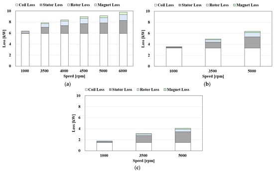
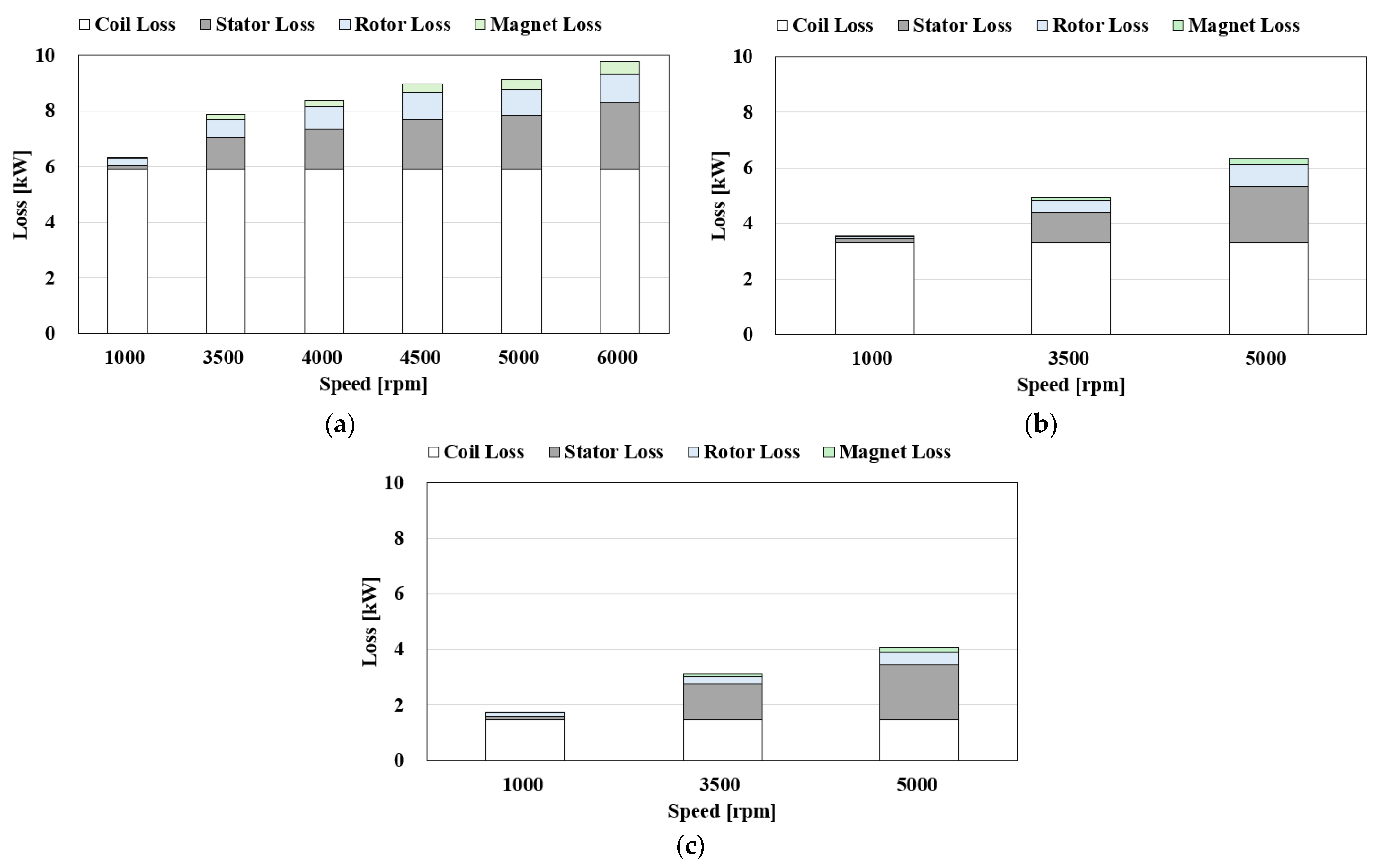
Figure 14 further decomposes the total electromagnetic loss shown in Figure 13d into coil, stator, rotor, and permanent-magnet losses. The individual loss components were determined based on the loss calculation methods described in Section 2. The coil loss was evaluated as stranded loss, the stator and rotor losses as core losses, and the permanent-magnet loss as solid loss resulting from induced eddy currents. The total electromagnetic loss was calculated as the sum of these individual loss components. Mechanical losses, including bearing friction and air resistance, were assumed to be negligible and were therefore not considered in the analysis. The coil copper loss decreased with decreasing input current, from 5.9 kW at 300 A to 3.3 kW at 225 A and 1.5 kW at 150 A. This behavior is attributed to the fact that copper loss is proportional to the square of the input current. The stator iron loss increased with rotational speed under all input-current conditions. At 300 A, the stator iron loss increased from 0.13 kW at 1000 rpm to 2.36 kW at 6000 rpm. The same trend was observed at 225 A and 150 A. This increase was primarily caused by the higher electrical frequency and greater magnetic flux variation at higher rotational speeds, which increased hysteresis and eddy-current losses. Magnet eddy-current loss also increased with increasing input current and rotational speed. At 300 A, magnet eddy-current loss increased from 0.01 kW at 1000 rpm to 0.45 kW at 6000 rpm. At 225 A and 150 A, the losses were relatively low because the alternating magnetic field in the magnets weakened as the input current decreased. Consequently, magnet eddy-current loss decreased.

Figure 14. Loss distribution analysis of motor components according to current magnitude variation: (a) 300 A, (b) 225 A, (c) 150 A.

3. Thermal Analysis

3.1. 3D Model and Properties

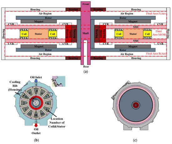
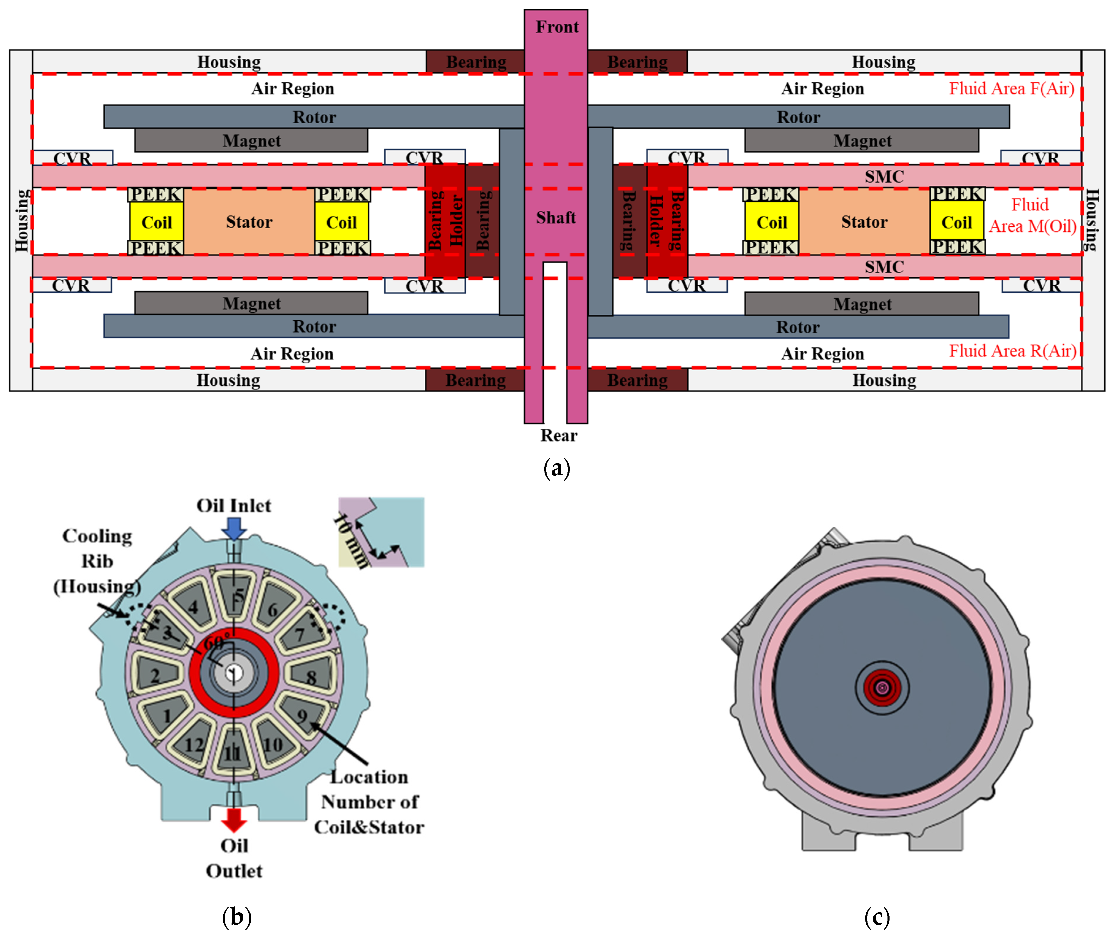
Figure 15 shows the overall structure of the AFM and the models used in this study. Figure 15a shows the overall motor structure, which consists of a stator, rotor, coil, soft magnetic composite (SMC), bearings, covers, bearing holders, shaft, and casing. The interior of the motor is divided into rotating and stationary regions. The rotor and magnets constitute the rotating region, through which air flows along the front and rear sides of the motor. In contrast, the stator and coils constitute the stationary region, where oil flows to cool the heat generated inside the motor. The SMCs are located at the top and bottom of the stator to prevent oil leakage and provide a magnetic flux path. Figure 15b shows the oil flow region of the base model, while Figure 15c shows the airflow region. In the oil-flow region, cooling ribs were symmetrically arranged at 60° on both sides of the central axis to cool the heat generated by the coil and stator. The materials and properties of the motor components used in the analysis are listed in Table 8. For the thermal-fluid analysis, the equivalent thermophysical properties of S45C were applied to the stator and rotor because complete thermophysical property data for VACOFLUX 17 and 50PN800 were unavailable from the manufacturers. The actual magnetic properties of VACOFLUX 17 and 50PN800 were used in the electromagnetic analysis. The shaft material was specified as stainless steel considering its mechanical durability and corrosion resistance under the internal operating environment of the motor. Although stainless steel has relatively low thermal conductivity compared with carbon structural steel, heat dissipation through the shaft was not considered a primary cooling path in the present cooling design. Therefore, the shaft material was not selected for thermal-performance enhancement. In addition, a comparative evaluation or optimization of shaft materials in terms of thermal conductivity, strength, corrosion resistance, magnetic characteristics, and thermal expansion was outside the scope of the present research, which focused on the electromagnetic characteristics and improvement of the oil- and air-cooling configurations.

Figure 15. AFM structure and 3D model (base model): (a) structural overview of the AFM, (b) oil area, (c) air area model.

Table 8. EV motor parts and materials.

Parts	Material	Density [kg/m3]	Thermal Conductivity [W/m·K]	Specific Heat [J/kg·K]	Viscosity [Pa·S]
Housing	Aluminum alloy	2790	168	833	-
Coil	Copper	8900	386	390
Stator	Steel S45C	7650	28	460
Magnet	NdFeB	7500	7.6	460
Cover ring	Aluminum alloy	2790	168	833
Rotor	Steel S45C	7650	28	460
Shaft	Stainless steel	8238	13.4	468
Bearing	Stainless steel	8055	15.1	480
PEEK	PEEK W6	1320	0.25	2.2
SMC	SMC	7581	5.3	450
Fluid area F&R	Air (gas)	1.225	0.026	1003.62	0.00001855
Fluid area M	PAO6 (Oil)	819.6	0.144	2289.2	0.0318

3.2. Mesh Settings and Boundary Conditions

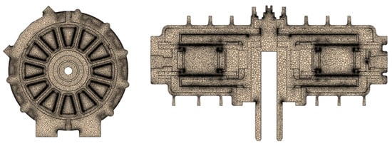
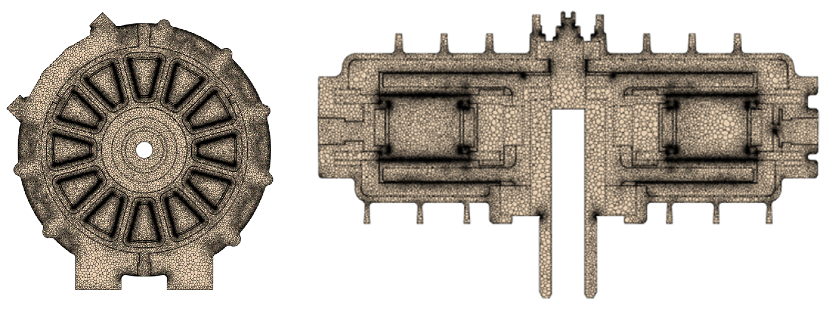
The numerical analysis in this study was based on three-dimensional steady-state thermal-fluid analysis. The standard k–ε turbulence model based on the Reynolds-averaged Navier–Stokes (RANS) equations was used. This model calculates turbulent viscosity using the turbulent kinetic energy (k) and its dissipation rate (ε) and provides stable predictions of internal flows in rotating machinery. It was selected for this study because of its low computational cost and good convergence characteristics. All thermal-fluid analyses were performed using the commercial CFD software STAR-CCM+(Ver. 19.06.008). A polyhedral mesh with a base size of 2 mm was used for the thermal-fluid analysis. Three prism layers with a total thickness of 0.4 mm were applied near the walls to resolve the near-wall flow and turbulence. Consequently, approximately 49 million computational cells were generated, as shown in Figure 16.

Figure 16. Mesh generation results of the AFM.

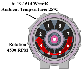
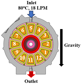
The boundary conditions for the motor thermal-fluid analysis are summarized in Table 9. The thermal-fluid analysis was performed under the maximum-output-power operating condition of 300 A and 4500 rpm. The heat generation rates of the individual motor components were determined based on electromagnetic losses calculated using ANSYS Maxwell under this operating condition. A one-way coupling approach was employed, in which the calculated electromagnetic losses were transferred to STAR-CCM+ as heat sources without considering temperature feedback to the electromagnetic model. The heat generation rates were 5913 W in the coils, 1780 W in the stator, 993 W in the rotor, and 290 W in the magnets, resulting in a total heat generation of 8976 W. To simulate heat transfer to the ambient air, a convective heat transfer coefficient of 19.1514 W/m²K was applied to the surfaces of the casing, shaft, and bearings. In addition, the Moving Reference Frame (MRF) method was applied to simulate the rotational motion of the rotor and magnets at 4500 rpm.

Table 9. Boundary conditions.

Part	Coil [W]	Stator [W]	Rotor [W]	Magnet [W]	Total Loss [W]
Heat source	5913	1780	993	290	8976
Region
Air			Oil

3.3. Fluid and Thermal Analysis Results

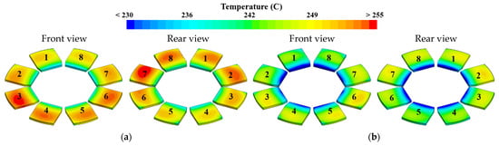
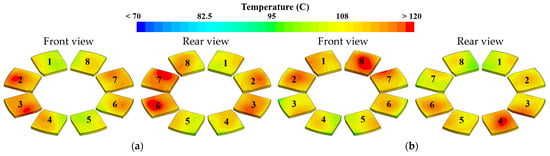
Among the thermal analysis results, permanent-magnet demagnetization was evaluated first because it is directly related to motor durability. Figure 17 shows the temperature distributions of the front and rear permanent magnets in the base model. Permanent magnets generally have an increased risk of demagnetization above 80 °C. Therefore, the magnet temperature was analyzed to determine whether it exceeded this limit. The results showed temperatures exceeding 230 °C in both the front and rear magnets, which were substantially higher than the specified demagnetization limit. In particular, the enclosed motor structure limits heat transfer to the outside environment, resulting in a continuous increase in magnet temperature. Prolonged exposure to high temperatures can cause irreversible demagnetization, reducing the residual magnetic flux density and magnetization performance. Consequently, torque and output power may decrease, potentially compromising the long-term durability of the motor. Therefore, improved cooling performance is necessary to ensure the thermal stability of permanent magnets.

Figure 17. Magnet temperature distribution of the base model: (a) front, (b) rear.

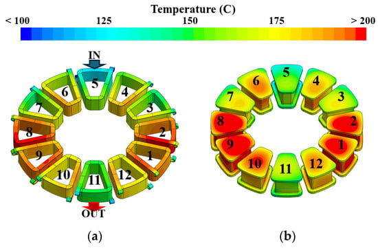
Figure 18 shows the temperature distributions of the coil and stator. Because the coils surround the stator, similar temperature distributions were observed at the same locations. High temperatures ranging from 170 °C to 200 °C were observed at coil and stator positions 1, 2, 8, and 9, while the average coil temperature ranged from 189 to 194 °C. The oil flow was concentrated near the center of the motor, resulting in insufficient oil supply to positions 1, 2, 8, and 9. Consequently, some coils exceeded the insulation coating temperature limit of 180 °C. Therefore, an improved cooling performance is required.

Figure 18. Coil and Stator temperature distribution of the base model: (a) coil, (b) stator.

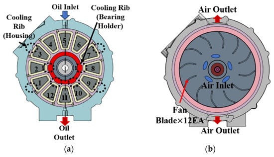
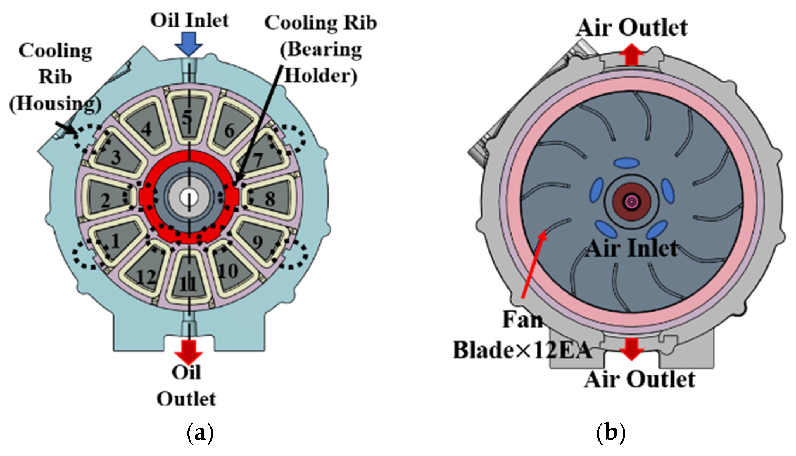
Based on these results, the R8+B12 model was designed to improve the cooling performance of the magnets and coils, as shown in Figure 19. In the model nomenclature, “R” denotes the cooling-rib configuration used to control and distribute the oil flow, whereas “B” denotes the rotor-blade configuration used to generate forced airflow. The R8 configuration consists of a total of eight cooling ribs: four ribs located in the outer housing region and four ribs installed around the bearing housing at the center of the motor. These ribs were arranged to redistribute the oil flow and improve the flow distribution among the coils. Figure 19a shows the oil-cooling structure. Four ribs were added to the bearing holder to improve the cooling balance between the coils. Additional ribs were added near coils 1 and 9 to prevent oil from flowing directly to the outlet and thereby improve the oil supply to the coils. The R8 configuration was developed through stepwise modification of the oil-flow path based on the CFD-predicted flow distribution. The number “8” indicates the number of cooling ribs in the final configuration and was not determined through a formal parametric optimization of the rib number. Figure 19b shows the cooling design of the airflow region. Twelve blades were placed at the top of the rotor. The blade shape was based on that of Company Y’s commercial motor. In addition, air inlets and outlets were designed to facilitate airflow. Five inlets were placed in the axial direction, while two outlets were located at the top and bottom of the motor. The number “12” indicates the number of rotor blades used in the B12 configuration. The blade number was selected considering the available rotor space and geometric arrangement. Therefore, the R8+B12 model represents a combined cooling configuration that integrates the improved oil-flow path of the R8 model with the forced-air cooling generated by the B12 rotor-blade model.

Figure 19. Improved cooling model (Configuration of the R8+B12 model): (a) cooling rib design (R8), (b) blade design (B12).

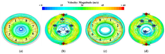
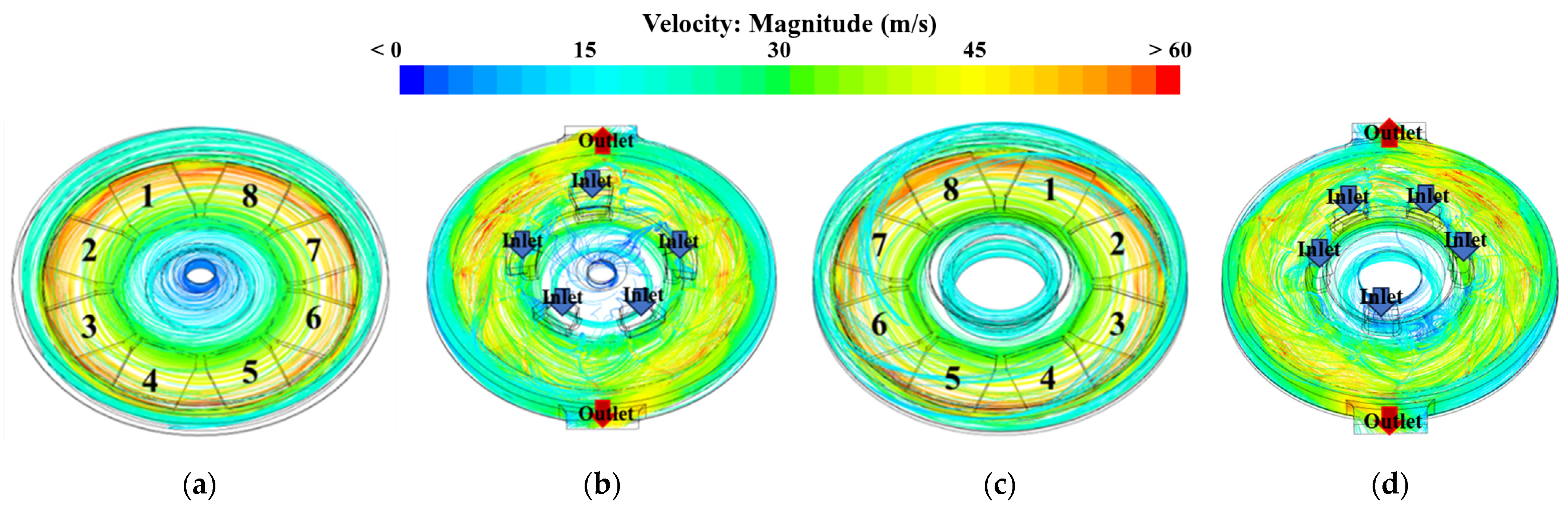
Figure 20 shows the streamlines in the airflow region. The Base model has a closed structure; therefore, air circulates inside the motor owing to rotor rotation. In contrast, the R8+B12 model incorporates rotor blades and air inlets and outlets in the housing. Outside air enters through the inlets, flows between the rotor and housing, and exits through the outlets. The calculated airflow rates were 750 LPM at the front and 720 LPM at the rear. This forced air circulation improved convective heat transfer around the rotor and permanent magnets, resulting in better magnet cooling compared with the Base model.

Figure 20. Streamline of the Air area: (a) base model at front, (b) R8+B12 model at front, (c) base model at rear, (d) R8+B12 model at rear.

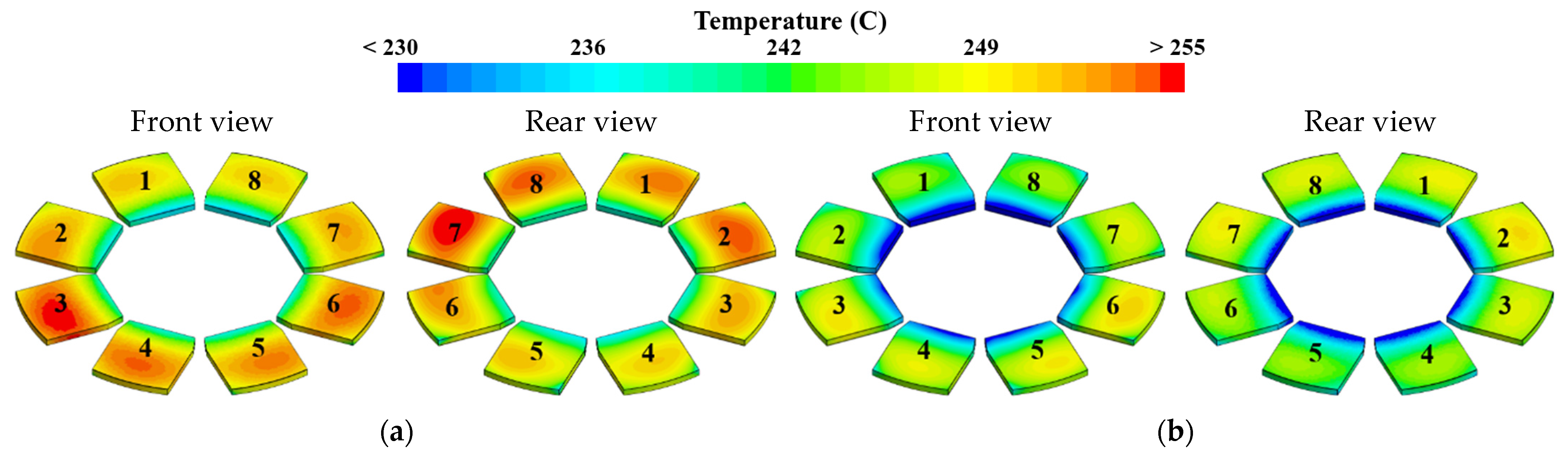
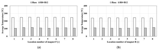
Figure 21 shows the permanent-magnet temperature distribution of the improved R8+B12 model. In the Base model, the magnet temperature exceeded 230 °C. In contrast, the blades, housing inlets, and outlets in the R8+B12 model improved airflow around the magnets. As a result, the magnet temperature decreased by more than 100 °C. Figure 22 compares the average magnet temperatures of the two models. In the Base model, all magnets showed a high average temperature of approximately 245 °C, indicating insufficient cooling performance. In the R8+B12 model, the average temperature of all magnets decreased to 110 °C, with only a small temperature difference among the magnets. The improved oil flow and air circulation increased heat transfer around the permanent magnets. However, the average temperature remained approximately 110 °C, which exceeded the recommended operating temperature of the permanent magnets. Therefore, further improvements in cooling performance are required.

Figure 21. Magnet temperature distribution of the R8+B12 model: (a) front, (b) rear.

Figure 22. Comparison of magnet average temperature: (a) front, (b) rear.

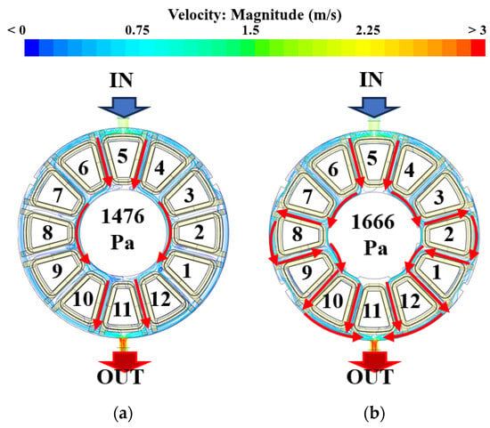
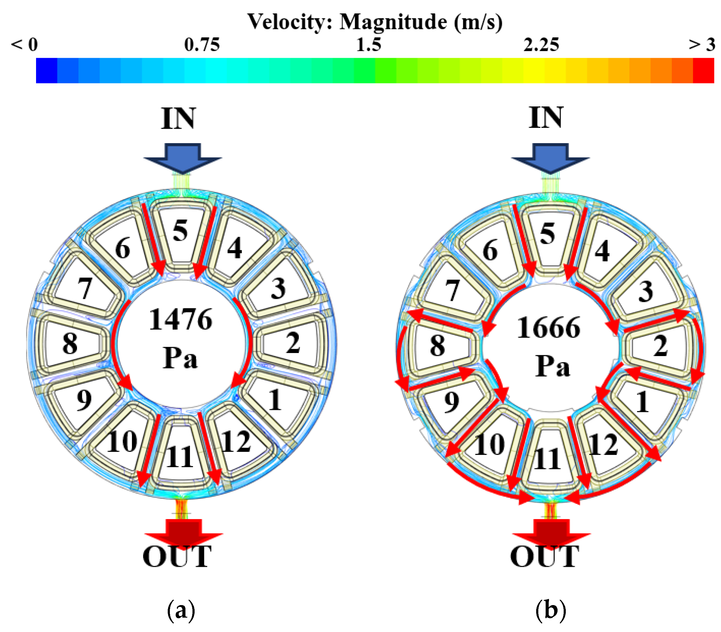
Figure 23 shows the velocity vectors in the oil flow regions of the Base and R8+B12 models. In the Base model, oil entered through the inlet and hit coil 5. It then flowed along both sides of the bearing holder and exited the outlet. The oil flow was primarily concentrated around coils 5 and 10–12, whereas relatively little oil reached coils 1–4 and 6–9. In contrast, the added ribs in the R8+B12 model redirected the oil flow direction and increased the flow rate around coils 1 and 9. In addition, a continuous flow path was formed through most of the coils, resulting in more uniform oil distribution than that of the Base model. The calculated pressure drops were 1476 Pa for the Base model and 1666 Pa for the R8+B12 model. Thus, the added ribs increased the pressure drop by 190 Pa, corresponding to a 12.9% increase relative to the Base model. Despite the increased pressure drop, the oil was distributed more uniformly throughout the coil and stator, thereby improving cooling performance.

Figure 23. Vector of oil area: (a) base model, (b) R8+B12 model.

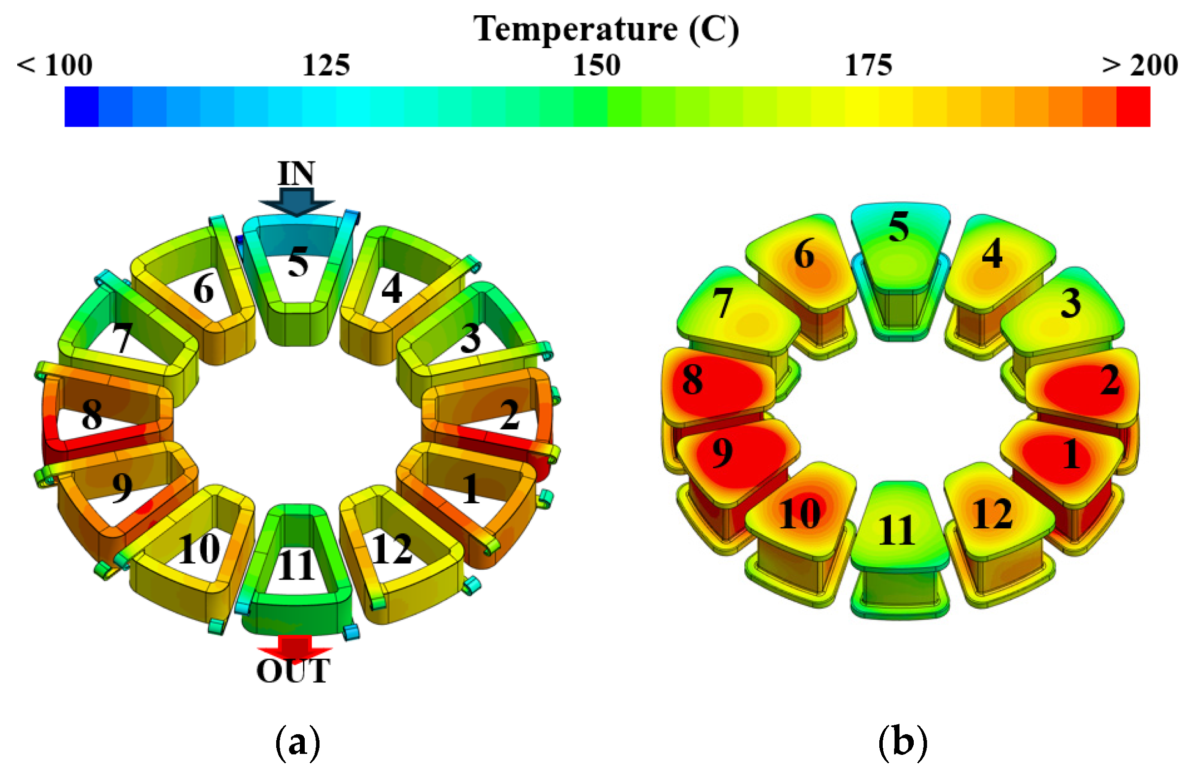
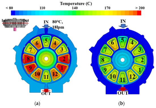
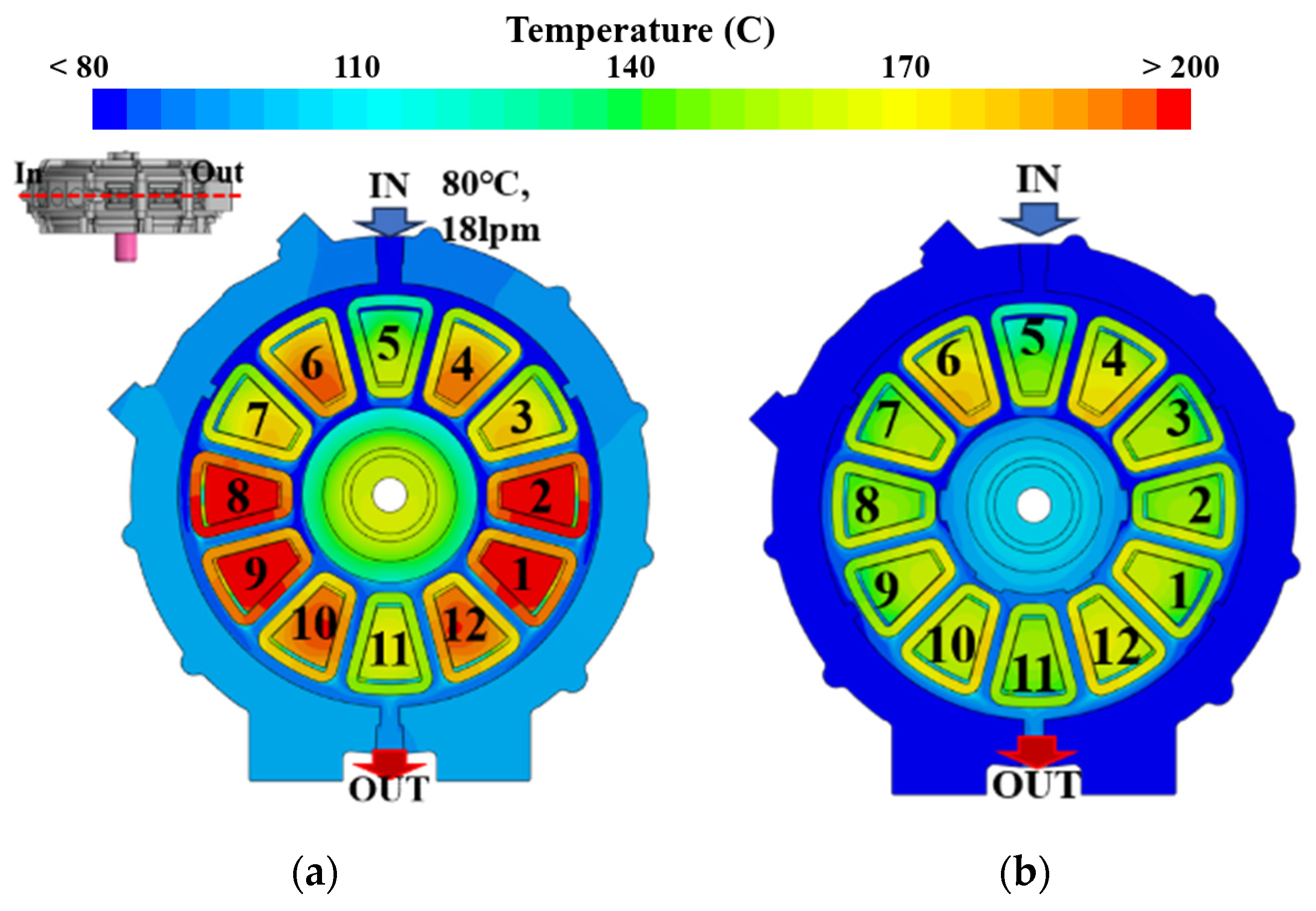
Figure 24 shows the temperature distributions at the center section of the motor, comparing coil and stator temperatures in the Base and R8+B12 models. In the Base model, high-temperature regions over 200 °C were observed throughout the coils and stator, particularly around coils 1–3 and 7–9. In contrast, the R8+B12 model eliminated the high-temperature regions above 200 °C. The maximum coil temperature decreased from approximately 194 °C to 170 °C, while the maximum stator temperature decreased significantly from 205 °C to 113 °C. In addition, the temperature distribution inside the motor became more uniform, indicating improved cooling performance of both the coils and stator. The improved oil flow path provided a more uniform oil supply to the coil and stator, thereby enhancing heat removal.

Figure 24. Temperature distribution of section M: (a) base model, (b) R8+B12 model.

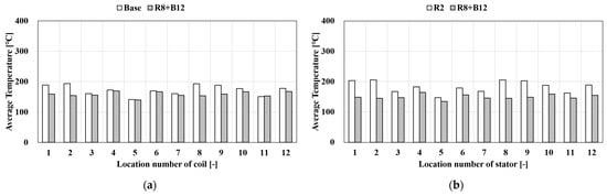
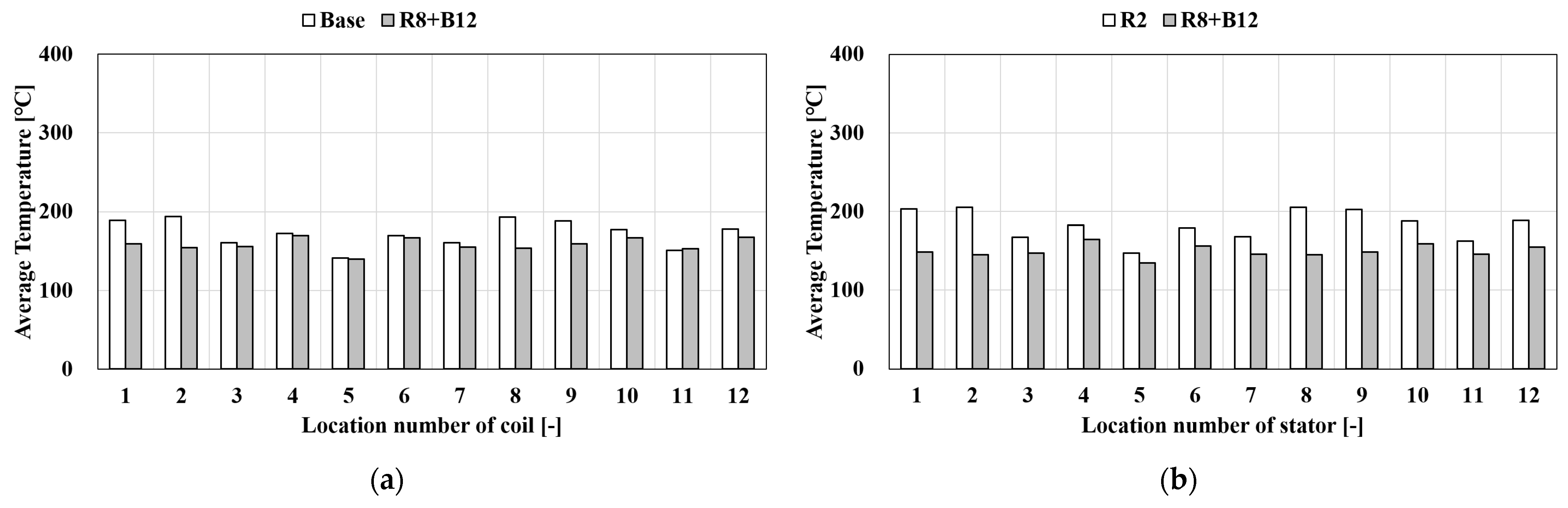
Figure 25 shows a quantitative comparison of the average coil and stator temperatures between the Base and R8+B12 models. As shown in Figure 25a, the coil temperatures of the Base model ranged from approximately 141 °C to 194 °C. In the R8+B12 model, the coil temperature decreased to approximately 140–170 °C. In particular, the temperatures of coils 1, 2, 8, and 9, which were relatively high in the Base model, decreased significantly. Consequently, the temperature difference between the coils was reduced. As shown in Figure 25b, the stator temperatures ranged from 147 °C to 205 °C in the Base model and decreased to 106–113 °C in the R8+B12 model. In addition, all stator positions in the R8+B12 model exhibited similar temperatures, indicating improved temperature uniformity. The standard deviations of the average temperatures were compared to quantitatively evaluate the temperature uniformity of the coil and stator. The standard deviation of the coil temperature decreased by approximately 50.6%, from 17.03 °C in the Base model to 8.42 °C in the R8+B12 model. Similarly, the standard deviation of the stator temperature decreased by approximately 58.6%, from 19.08 °C to 7.89 °C. These results indicate that the temperature differences between the positions were significantly reduced in the R8+B12 model. The improved oil flow path provided a more uniform oil supply to the coil and stator. Therefore, the R8+B12 model improved not only the average temperature but also the cooling uniformity.

Figure 25. Comparison of coil and stator average temperature: (a) coil, (b) stator.

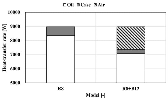
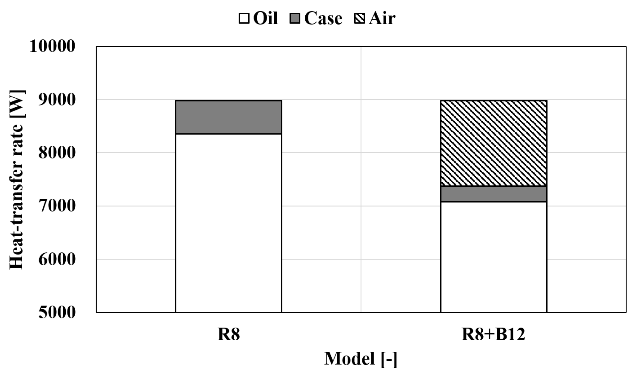
Figure 26 compares the heat transfer through the different cooling paths in the Base and R8+B12 models. In the Base model, heat transfer through the oil was 8324.6 W, accounting for most of the total heat transfer, while natural convection through the casing was 651.9 W. In contrast, in the R8+B12 model, heat transfer through the oil decreased to 7078.7 W, and heat transfer through the casing decreased to 291.2 W. However, heat transfer through the air cooling increased to 1606.6 W due to the addition of the blades and the resulting airflow. These results indicate that some of the heat transferred through the oil in the Base model was instead transferred through the air in the R8+B12 model. Therefore, the R8+B12 model uses both oil and air cooling, resulting in improved thermal management of the motor.

Figure 26. Comparison of heat transfer rate.

4. Conclusions

In this study, a multi-physics analysis combining electromagnetic and thermal-fluid analyses was conducted for an SSDR AFM with a target output power of 160 kW for electric vehicles. The electromagnetic performance and thermal management characteristics were analyzed. In addition, the improvement in thermal management performance achieved by the modified cooling flow path was evaluated. The main findings are as follows:

• Three-dimensional electromagnetic analysis was conducted to analyze the back EMF and cogging torque. The back EMF exhibited a symmetrical waveform with a phase difference of 120°. The cogging torque exhibited periodic variations, with a maximum value of approximately 8 Nm, attributed to the slot pitch. These results confirmed the basic electromagnetic characteristics of the AFM.
• The output power and torque were analyzed by considering the inverter voltage limit. At 450 A, the 700 V voltage limit was satisfied at current phase angles of 10.5° at 4130 rpm, 28° at 5000 rpm, and 50° at 6000 rpm. At 300 A, the voltage limit was satisfied at 10° at 5000 rpm and 20° at 6000 rpm. However, the torque decreased as the current phase angle increased, indicating a trade-off between the voltage limit and torque performance.
• The efficiency and loss characteristics were analyzed at different input currents. At 300 A, the motor achieved an output power of 150 kW with an efficiency of approximately 94%. At 450 A and 6000 rpm, the stator iron loss, rotor iron loss, and permanent magnet eddy-current loss accounted for approximately 12%, 10%, and 6% of the output power, respectively. These increased losses were the main cause of efficiency reduction at high speeds.
• In the Base model, the oil flow was concentrated near some coils, resulting in large temperature differences between the coil and stator positions. The maximum temperatures of the coil and stator were about 194 °C and 205 °C, respectively, while the average magnet temperature was approximately 245 °C. These temperatures exceeded the allowable limits of the coil insulation and permanent magnets. Therefore, the nonuniform cooling flow was identified as a major factor limiting the thermal management performance of the Base model.
• The R8+B12 model improved the oil and airflows, resulting in a more uniform cooling flow around the coil and stator. Compared with the Base model, the maximum coil temperature decreased from 194 °C to 170 °C, while the maximum stator temperature decreased from 205 °C to 113 °C. In addition, the standard deviations of the coil and stator temperatures decreased by approximately 50.6% and 58.6%, respectively.
• In the Base model, approximately 92.7% of the total heat was removed by the oil. In the R8+B12 model, approximately 78.9% was removed by oil, 17.9% by air, and 3.2% by the casing. The blades, housing inlets, and outlets increased air cooling and distributed heat transfer from the oil to the air region. Therefore, effective thermal management of high-power AFM requires consideration of forced airflow using fans or blades in addition to oil cooling.

References

- Demartini, M.; Ferrari, M.; Govindan, K.; Tonelli, F. The transition to electric vehicles and a net zero economy: A model based on circular economy, stakeholder theory, and system thinking approach. J. Clean. Prod. 2023, 410, 137031. [Google Scholar] [CrossRef] [Scilit]
- Pavlínek, P. Transition of the automotive industry towards electric vehicle production in the east European integrated periphery. Empirica 2023, 50, 35–73. [Google Scholar] [CrossRef] [Scilit]
- Petavratzi, E.; Gunn, G. Decarbonising the automotive sector: A primary raw material perspective on targets and timescales. Miner. Econ. 2023, 36, 545–561, Correction in Miner. Econ. 2023, 36, 743. https://doi.org/10.1007/s13563-022-00351-1. [Google Scholar] [CrossRef] [Scilit]
- Diouf, B. The electric vehicle transition. Environ. Sci. Adv. 2024, 3, 332–345. [Google Scholar] [CrossRef] [Scilit]
- Chan, C.C.; Han, W.; Tian, H.; Liu, Y.; Ma, T.; Jiang, C.Q. Automotive revolution and carbon neutrality. Front. Energy 2023, 17, 693–703. [Google Scholar] [CrossRef] [Scilit]
- Sanguesa, J.A.; Torres-Sanz, V.; Garrido, P.; Martinez, F.J.; Marquez-Barja, J.M. A review on electric vehicles: Technologies and challenges. Smart Cities 2021, 4, 372–404. [Google Scholar] [CrossRef] [Scilit]
- Blázquez Lidoy, J.; Martín Moreno, J.M. Eficiencia energética en la automoción, el vehículo eléctrico, un reto del presente. Econ. Ind. 2010, 377, 76–85. [Google Scholar]
- Credo, A.; Tursini, M.; Villani, M.; Di Lodovico, C.D.; Orlando, M.; Frattari, F. Axial flux PM in-wheel motor for electric vehicles: 3D multiphysics analysis. Energies 2021, 14, 2107. [Google Scholar] [CrossRef] [Scilit]
- Huang, R.; Liu, C.; Song, Z.; Zhao, H. Design and analysis of a novel axial-radial flux permanent magnet machine with Halbach-array permanent magnets. Energies 2021, 14, 3639. [Google Scholar] [CrossRef] [Scilit]
- Wang, H.; Zeng, X.; Eastham, J.F.; Pei, X. Axial flux permanent magnet motor topologies magnetic performance comparison. Energies 2024, 17, 401. [Google Scholar] [CrossRef] [Scilit]
- Johansen, P.R.; Patterson, D.; O’Keefe, C.; Swenson, J. The use of an axial flux permanent magnet in-wheel direct drive in an electric bicycle. Renew. Energy 2001, 22, 151–157. [Google Scholar] [CrossRef] [Scilit]
- Hao, Z.; Ma, Y.; Wang, P.; Luo, G.; Chen, Y. A review of axial-flux permanent-magnet motors: Topological structures, design, optimization and control techniques. Machines 2022, 10, 1178. [Google Scholar] [CrossRef] [Scilit]
- Cavagnino, A.; Lazzari, M.; Profumo, F.; Tenconi, A. A comparison between the axial flux and the radial flux structures for PM synchronous motors. IEEE Trans. Ind. Appl. 2002, 38, 1517–1524. [Google Scholar] [CrossRef] [Scilit]
- Tsunata, R.; Takemoto, M.; Ogasawara, S.; Watanabe, A.; Ueno, T.; Yamada, K. Development and evaluation of an axial gap motor using neodymium bonded magnet. IEEE Trans. Ind. Appl. 2018, 54, 254–262. [Google Scholar] [CrossRef] [Scilit]
- Chen, X.; Shen, Q.; Wang, D.; Han, L. Thermal comparison of axial and radial flux permanent magnet motor with the same volume. In Proceedings of the 2019 22nd International Conference on Electrical Machines and Systems (ICEMS), Harbin, China, 11–14 August 2019. [Google Scholar] [CrossRef] [Scilit]
- Akar, M.; Eker, M.; Özsoy, M.; Gerçekçioğlu, H.S. Efficiency Analysis of Axial Flux SynRM in Vairable Speed Applications. Machines 2022, 10, 838. [Google Scholar] [CrossRef] [Scilit]
- Gadiyar, N.; Van Verdeghem, J.V.; Severson, E.L. A review of axial flux permanent magnet machine technology. IEEE Trans. Ind. Appl. 2023, 59, 3920–3933. [Google Scholar] [CrossRef] [Scilit]
- Cheng, D.K. Plane electromagnetic waves. In Field and Wave Electromagnetics, 2nd ed.; Addison-Wesley: Boston, MA, USA; Tsinghua University Press: Beijing, China, 2007; pp. 378–388. [Google Scholar]
- Slutskiy, D.; Aung, S.H.; Basnet, S. Comparison of axial and radial flux permanent magnet machines. In Proceedings of the 2022 North American Power Symposium (NAPS), Salt Lake City, UT, USA, 9–11 October 2022. [Google Scholar] [CrossRef] [Scilit]
- Shen, Q.; Wu, X.; Zhu, H.; An, P.; Zeng, Y.; Zhong, Y.; He, L. Design of Spray Cooling System for YASA AFPM Flat Wire Winding Motors. Int. Commun. Heat Mass Transf. 2025. Available online: https://ssrn.com/abstract=5364071 (accessed on 23 July 2025).
- Chen, H.; Xiao, J.; Huang, Y.; He, P.; Zhang, J. Cooling enhancement of axial flux permanent magnet motors by corrugated spiral channels with nanofluid. J. Electr. Eng. Technol. 2025, 20, 1523–1540. [Google Scholar] [CrossRef] [Scilit]
- Gao, P.; Ren, H.; Wang, X.; Wang, L.; Zhao, X. Design of cooling structure for yokeless and segmented armature axial flux permanent magnet machine based on computational fluid dynamics. IEEE Trans. Energy Convers. 2026, 41, 975–989. [Google Scholar] [CrossRef] [Scilit]
- Zhao, X.; Shuai, Z.; Zhang, Y.; Li, Q. Design and research of high torque density AFPMSM based on hybrid cooling method. In Proceedings of the 2025 IEEE 8th International Electrical and Energy Conference (CIEEC), Changsha, China, 16–18 May 2025. [Google Scholar] [CrossRef] [Scilit]
- Qiao, L.; Liu, A.; Ren, D.; Meng, F.; Wang, Y.; Liu, Y. Cooling system design and temperature field analysis for high-speed switched reluctance motor considering multi-field coupling of electromagnetic-thermal-flow. IEEE Access 2025, 13, 77196–77209. [Google Scholar] [CrossRef] [Scilit]
- Su, X.; Li, F.; Yin, Z.; Liu, X.; Zhao, H. Order-reduced nonlinear semi-analytical multiphysics model for axial-flux motors. IEEE Trans. Transp. Electrif. 2025, 11, 10188–10202. [Google Scholar] [CrossRef] [Scilit]
- Qiu, J.; Zhang, Z.; Zhu, Z.; Luo, C. Design and optimization of honeycomb cooling structure for hybrid electric vehicle oil-cooled motor. Appl. Therm. Eng. 2025. Available online: https://ssrn.com/abstract=5391904 (accessed on 14 August 2025).
- Jenkins, C.; Jones-Jackson, S.; Zaher, I.; Pietrini, G.; Rodriguez, R.; Cotton, J.; Emadi, A. Innovations in axial flux permanent magnet motor thermal management for high power density applications. IEEE Trans. Transp. Electrif. 2023, 9, 4380–4405. [Google Scholar] [CrossRef] [Scilit]
- Wang, R.-J.; Kamper, M.J.; Van der Westhuizen, K.; Gieras, J.F. Optimal design of a coreless stator axial flux permanent-magnet generator. IEEE Trans. Magn. 2005, 41, 55–64. [Google Scholar] [CrossRef] [Scilit]
- Um, D.-Y.; Kumar, R.; Nadkin, A.; Batra, T.; Sjöberg, L. Performance enhancement of YASA axial flux permanent magnet machines using soft magnetic composites with reduced eddy current losses. In Proceedings of the 2025 28th International Conference on Electrical Machines and Systems (ICEMS), Busan, Republic of Korea, 16–19 November 2025; pp. 109–114. [Google Scholar] [CrossRef] [Scilit]
- Polikarpova, M.; Lindh, P.; Gerada, C.; Rilla, M.; Naumanen, V.; Pyrhönen, J. Thermal effects of stator potting in an axial-flux permanent magnet synchronous generator. Appl. Therm. Eng. 2015, 75, 421–429. [Google Scholar] [CrossRef] [Scilit]
Disclaimer/Publisher’s Note: The statements, opinions and data contained in all publications are solely those of the individual author(s) and contributor(s) and not of MDPI and/or the editor(s). MDPI and/or the editor(s) disclaim responsibility for any injury to people or property resulting from any ideas, methods, instructions or products referred to in the content. |
© 2026 by the authors. Licensee MDPI, Basel, Switzerland. This article is an open access article distributed under the terms and conditions of the Creative Commons Attribution (CC BY) license.