


Abstract
Heating, ventilation and air-conditioning (HVAC) systems are a major source of hotel energy use, particularly in tropical climates, but evidence on Internet of Things (IoT)-based control under real hotel operation remains limited. This study field-evaluated a commercial, interoperable IoT platform for reducing HVAC energy use in a guest room of a four-star resort in Cozumel, Mexico. Four intelligent control scenarios were implemented with IoT devices: an infrared controller, door/window and motion sensors, a presence sensor, a temperature-humidity sensor, and a Zigbee gateway bridged to the hotel Wi-Fi network. Indoor and outdoor conditions were recorded hourly over 44 valid 24 h periods, divided equally between a baseline period and an intelligent-control period, and HVAC energy consumption was estimated, without electrical metering, with a rule-based thermal-response model based on indoor temperature, relative humidity, and the outdoor–indoor temperature difference. With outdoor temperature higher by 1.6 °C and outdoor relative humidity higher by 3.8 percentage points during the intervention, estimated HVAC energy consumption decreased by 30.3% (95% CI: 10.9–45.6%), from 943.6 kW h to 657.3 kW h; this is an unadjusted difference between two sequential periods. When the intervention occupied- and unoccupied-hour energy rates were standardised to the baseline occupancy mix, the corresponding reduction was 26.3%. The confidence interval applies to the unadjusted one-room period contrast and is not adjusted for occupancy or outdoor weather conditions. Routine over-cooling was reduced and no guest complaints were recorded. The observed period difference was associated mainly with changes in the timing and estimated load of HVAC operation rather than with a uniform reduction in cooling demand: operating hours fell by only 6.8%, and the reduction in mean hourly estimated HVAC energy was greater during unoccupied than occupied periods. Differences in occupancy composition also contributed to the whole-period contrast. Scenario activation frequency was not proportional to estimated energy demand and so cannot serve as a proxy for scenario effectiveness; isolating the contribution of individual scenarios would require scenario-specific measurement. The study completed the first three of the five framework stages (scenario definition, IoT data acquisition and performance evaluation) in one guest room. The results are specific to this room, period and operating conditions, should not be generalised to other hotels or climates, and require validation against metered HVAC electricity.
1. Introduction
The building sector represents approximately 40% of global energy consumption and approximately one-third of energy-related carbon emissions [1]. The hospitality sector faces increasing pressure to reduce its environmental footprint [2], particularly its energy-related carbon emissions. This challenge is especially relevant for hotels operating in tropical and subtropical climates, where persistently high temperatures and humidity create substantial cooling and dehumidification demands to maintain comfortable indoor conditions for guests [2,3]. Heating, ventilation, and air-conditioning systems (HVAC) account for a substantial share of hotel energy consumption, making them a major target for reducing operating energy costs and carbon emissions related to energy [4,5]. Optimising HVAC operation has therefore become a key strategy for improving energy efficiency, advancing building decarbonisation, and promoting sustainable hotel management.
Hotels have distinctive operational characteristics compared to conventional buildings due to the wide variety of spaces, equipment, and HVAC installations involved. Guest comfort is the top priority regardless of outdoor conditions, unlike offices or schools, which can prioritise operational efficiency. HVAC performance depends on outdoor conditions, system characteristics, operational practices, occupancy, and guest/occupant behaviour. Even identical rooms equipped with the same system can show markedly different consumption patterns, because guests interact with the equipment in different ways [6,7]. This effect is more pronounced in tropical climates, where HVAC systems must control cooling and humidity simultaneously [3,4,8], increasing compressor operating time and electricity demand.
Hotel energy performance cannot be fully characterised by energy consumption or equipment efficiency alone; a more comprehensive assessment should also consider indoor environmental conditions, occupancy patterns, occupant behaviour, and actual HVAC operation under real-world conditions [9,10]. Hotel guests are generally not directly responsible for the energy costs incurred during their stay and tend to have poorer energy-conservation behaviour than in residential settings, reducing incentives to avoid unnecessary consumption [7,11]. Guest-room energy waste can arise from low temperature settings and air-conditioning operation while doors remain open [12], while occupancy-based studies also show that substantial energy use can persist during unoccupied periods [6]. In this context, IoT-based HVAC control systems can integrate environmental and occupancy data, such as temperature, humidity, and presence, to dynamically adjust air-conditioning operation and reduce unnecessary energy consumption [9,13,14].
Building energy technologies, the Internet of Things (IoT), artificial intelligence (AI), smart control systems, and real-time monitoring are now well established in building energy management. These technologies support monitoring, control, and data-driven optimisation, key strategies to reduce energy demand and improve efficiency [9,10,13,15,16]. By integrating information from the physical environment, these technologies enable intelligent control based on continuous monitoring and data-informed decision making. Despite these advances, evaluating their performance under real hotel operating conditions remains methodologically difficult.
Simulation models remain widely used at the design stage [17,18]. However, the simplifications required to represent occupancy and building operation can produce discrepancies between simulated and actual energy performance. Such assumptions suit design optimisation but cannot fully represent hotel operation—where HVAC demand varies with guest preferences, occupancy patterns, housekeeping activities, door and window operation, and changing outdoor conditions. Methodologies developed and validated exclusively using simulations, aggregated consumption data, or conventional building settings should therefore not be assumed to transfer directly to hospitality applications without accounting for these differences [6,19].
Continuous monitoring has substantially improved HVAC evaluation, with interconnected IoT sensors and automated systems that allow the collection of environmental, operational, and occupancy data in real time [9,10]. However, the practical value of these hospitality datasets depends on evaluation methodologies that select relevant performance indicators and turn the measured data into meaningful information for energy management [9,10,16]. This reveals a larger methodological gap: although continuous monitoring is increasingly available, the hospitality literature still lacks a standardised evaluation framework that defines which variables and performance indicators should be monitored and how intelligent HVAC performance should be consistently assessed and compared in hospitality contexts. Existing studies frequently report energy-savings results or proposed implementations, but provide limited guidance for objectively assessing their effectiveness or determining whether intelligent HVAC control produces measurable and economically significant improvements under real hotel operating conditions [20].
Addressing this challenge requires moving beyond data acquisition alone towards an integrated evaluation methodology. Smart HVAC performance should not be assessed only by electricity consumption. Other factors in the real-world context (such as relevant environmental, operational, occupant behaviour and economic variables) should be included in the performance analysis using a systematic framework capable of providing objective and reproducible evidence [9,21]. Evaluation also requires explicitly defined operational scenarios. Although IoT-based platforms respond automatically to sensor information, their performance depends on multivariable decision rules rather than a single trigger condition: examples in the literature combine occupancy information with indoor environmental variables and, in some cases, door-state or outdoor-condition data to define automated control rules [14,17,22]. However, operational scenarios and their underlying decision rules are not always reported in sufficient detail, which can limit methodological transparency and hinder the reproducibility and comparison of intelligent HVAC interventions [20].
The authors’ previous systematic review on the maturity of research on intelligent energy-efficiency systems for hotel rooms identified four methodological gaps in this field [20]. First, there is no clear consensus on which variables to monitor when evaluating smart HVAC systems in hospitality applications, and previous work reports fragmented approaches to variable selection and unclear monitoring objectives. Second, standardised indicator systems that integrate operational, environmental, behavioural, technical, connectivity, and economic dimensions simultaneously remain scarce. Third, operational scenarios are often described in insufficient methodological detail, making reported implementations difficult to reproduce or compare. Finally, longitudinal evidence obtained under real hotel operating conditions remains limited, despite being essential for evaluating the long-term performance of intelligent HVAC control strategies. This study does not re-examine these gaps as a literature question; it tests, in one hotel guest room, whether a framework built on them can be operated in the field. It specifies the monitored variables and indicators, documents each control scenario with its thresholds and operating hours, and reports hourly field data from a baseline period and an intervention period.
To address these limitations, this study proposes an integrated methodological framework for evaluating smart HVAC systems in hotel rooms. The framework was developed from the gaps identified in the systematic review [20] and demonstrated through a longitudinal field implementation under real hotel operating conditions. Rather than assessing performance through energy consumption alone, it combines relevant environmental, operational, behavioural, technical, and economic variables with performance indicators in a unified procedure—allowing an objective and reproducible evaluation of intelligent HVAC performance in real operation.
Previous studies have demonstrated occupancy-responsive climate control and occupancy-dependent energy use in real hotel guest rooms [6,14]. Instead of presenting occupancy-based control, this study presents an integrated evaluation framework in a hotel guest room and demonstrates the implementation of the framework in real-world scenarios. The methodology combines environmental and occupancy detection, explicit multivariable HVAC control rules, operational scenarios, and environmental, energy, emissions, economic, and reliability indicators within a longitudinal baseline-intervention evaluation. This provides a structured and reproducible approach for evaluating intelligent HVAC performance under real hotel operating conditions.
2. Materials and Methods
2.1. Framework Design
Figure 1 presents the conceptual framework proposed to evaluate energy savings in smart hotel rooms under intelligent HVAC control. The framework comprises five stages linked by an iterative optimisation loop. The first stage defines the control scenarios: the set points of target temperature and humidity, their minimum and maximum limits, and the operating time window of each scenario are agreed with the hotel. For this study and performance evaluation, the predefined operating range was 23.5 to 25.0 for indoor temperature and 60–75% RH for indoor relative humidity. These ranges were used as performance criteria and were distinct from the operational trigger thresholds used by individual control scenarios. In particular, Scenario 3 was activated at RH , introducing a 2.5 pp band above the 75% RH target boundary. This threshold was selected as an operational design choice to avoid repeated HVAC commands in response to small or transient humidity excursions associated with room-access events. The choice was also informed by the baseline indoor RH, which averaged approximately 77.3%. Thus, Scenario 3 would respond to more pronounced humidity conditions than to every minor excursion that exceeds the target range.
Figure 1.
Conceptual framework for evaluating energy savings in smart hotel rooms with intelligent HVAC control. Only Stages 1–3 were carried out in this study. The Stage 3 evaluation criteria were indoor temperature within 23.5–25 , indoor relative humidity within 60–75% RH, and the absence of control-related guest complaints. Because these criteria were not all satisfied, Stage 4 (optimisation), Stage 5 (final configuration), and the return loop were not carried out in this study.
The second stage is IoT data acquisition. An initial commissioning period of at least 24 confirms sensor connectivity, data integrity, and communication stability, verifies the correct execution of every scenario, and establishes the placement of each sensor and controller. The room is then monitored under two conditions: a baseline period without intelligent control and an intervention period with the scenarios active. Each period should last at least 20 days. Environmental, operational, and HVAC-related variables are recorded hourly; outdoor conditions are retrieved from a meteorological API, and guest complaints are logged hourly.
The third stage is performance evaluation. Performance indicators are calculated from the consolidated dataset and the baseline and intervention periods are compared. Predefined criteria include maintaining indoor predefined temperature/RH target ranges, reducing over-cooling, estimated HVAC operation load, energy consumption, and associated CO2 emissions, and ensuring no deterioration in system reliability or guest comfort, indicated in this stage by the absence of complaints. If these criteria are met, the configuration is considered technically validated for the room in which it was evaluated; at this point, the sensing architecture and control logic are not modified further (final configuration). Application to other rooms requires a separate pass through Stages 1–3 in those rooms.
In this study, only Stages 1–3 were implemented and evaluated. Stages 4 and 5 represent the subsequent steps proposed in the framework and were not experimentally tested. If the Stage 3 criteria are not met in future applications, the framework is intended to proceed to an optimisation in Stage 4. In that stage, potentially redundant devices or scenarios may be identified, additional sensing may be introduced where needed, and the control logic may be refined by examining areas of the room not covered by the sensors and operating situations not anticipated in the first stage. Possible refinements include requiring all predefined conditions to be satisfied simultaneously before a scenario executes, relaxing conditions to tune the activation frequency, adding operating time windows, or adjusting the temperature thresholds that trigger the scenarios. The revised configuration would then return to the scenario-definition stage for re-evaluation before a final configuration is established.
2.2. Indicators
The control scenarios were designed to respond to specific environmental and occupancy conditions, drawing on the indicators identified in the previous review of the literature by the authors [20]. Table 1 presents the full set of indicators for this study, grouped by category, with the unit and the data source for each indicator. Rather than reproducing the full set of indicators identified in the literature, indicator selection therefore prioritised variables that were directly measurable in the room or could support the estimation of HVAC energy use without requiring direct electrical metering. Subsequently, the selected indicators were organised into six functional categories: comfort, HVAC operation, energy, environmental, economic, and reliability, to provide a structured assessment of the proposed hospitality control strategy.
Table 1.
Indicator system proposed for the evaluation of IoT-based intelligent HVAC control in hotel rooms.
The indicator system has two functions. First, a set of monitored variables describes the current room conditions and serves as input to determine whether a control scenario should be activated and, if so, which one: indoor temperature and humidity, occupancy status and time of day. Second, the resulting indicators are used to evaluate the performance and outcomes of the control strategy in terms of comfort, HVAC operation, energy use, environmental impact, economic performance, and reliability. The system therefore links environmental sensing to control logic and performance evaluation, forming a continuous sequence from room-state assessment through HVAC intervention to its operational, environmental, and economic effects. These indicators define the design constraints of the smart room. The primary objective is to maximise energy efficiency without compromising guest comfort or creating complaints. Meeting this objective requires the control system to keep the monitored conditions within the preferred ranges. Daytime control scenarios (Scenarios 1 and 4) operated from 09:00 to 20:00, while Scenarios 2 and 3 remained continuously active. For each hourly observation, deviation from the predefined target range was calculated as the distance to the nearest boundary when the observation fell outside the target range, and as zero when it remained within the target range. Temperature deviation was therefore calculated as
and relative-humidity deviation as
The phase-level indicators reported in Table 3 were calculated as the arithmetic mean of the corresponding hourly deviations. Temperature deviation is reported in , whereas relative-humidity deviation is reported in percentage points (pp).
2.3. Control Scenarios
The smart-control logic used two air-conditioning modes: cool and dry. In Cool mode, the unit regulates room temperature towards the selected set point; in dry mode, it prioritises humidity reduction while limiting unnecessary cooling. Three of the four scenarios used dry mode. Because inverter compressor operation is continuously modulated according to thermal load, indoor conditions, set point, and operating mode, neither mode was assumed to correspond to a fixed compressor power level.
These indicators shape the control scenarios investigated in this study, listed in Table 2. Scenario 1, for example, applies when the room is unoccupied during the day (09:00–20:00): the controller raises the commanded set point to 24 and switches the unit to dry mode (dehumidification). The 77.5% RH threshold used in Scenario 3 should therefore be interpreted as an operational activation threshold rather than as the upper limit of the target humidity range. The 60–75% RH interval remained the predefined performance target. The 2.5 pp separation above the target boundary was introduced as a control band to reduce repeated scenario activation during short-duration humidity increases, particularly those associated with room-access events. Because the baseline mean indoor RH was approximately 77.3%, setting the trigger directly at 75% would have made Scenario 3 eligible for activation under a large proportion of the normal baseline conditions in the room. The 77.5% RH threshold was therefore not statistically optimised but was selected as a practical control parameter for field implementation.
Table 2.
Smart control scenarios. Each scenario adjusts the air-conditioning unit to a temperature, T, in either cool or dry mode when its condition is met.
Each scenario thus defines the system’s sensing and, in turn, the minimum set of IoT devices needed for reliable operation at the lowest installation cost and complexity. The temperature and humidity sensor continuously monitors indoor conditions and triggers an evaluation whenever it detects a change in room temperature of at least or 1 pp of relative humidity. When the indoor temperature falls below the Scenario 4 trigger threshold of 22 , the sensor notifies the gateway, which instructs the IR controller to set the unit to 24 ; this scenario operates during the day and is disabled at night. Each opening or closing event registered by the door and terrace contact sensors also triggers an indoor temperature evaluation, prompting the gateway to command the IR controller to restore the commanded set point to 24 only when the scenario condition is satisfied. While the terrace door remains open, the unit switches to dry mode at a commanded set point of 24 , reducing excess moisture while limiting unnecessary cooling.
If all three conditions were satisfied (an exact hourly timestamp, no PIR detection during the preceding 15 min, and no presence detected by the mmWave sensor at that moment), the IR controller triggered the corresponding HVAC adjustment to dry mode at 24 . If the conditions for Scenario 4 were also met, Scenario 4 was executed first, followed by Scenario 1 once the hourly absence conditions were satisfied. These scenarios are intended for hotels where the air conditioning runs continuously, a standard practice in hot, humid destinations, except when guests turn off the unit. In this context, the control logic reduces unnecessary cooling and energy use while maintaining the goal of the set temperature for thermal comfort without restricting the ability of the guests to adjust the HVAC settings manually.
2.4. Sensors and IoT System
The IoT system was designed on the basis of the hotel’s practical constraints: control of temperature and humidity, minimal battery dependency, low data consumption, full compatibility with a free and openly accessible IoT platform. These constraints favoured interoperability, connectivity, and replicability over a proprietary ecosystem while preserving the aesthetics of the room. Figure 2 shows a floor plan of the guest room and the layout of the seven physical devices that represent six types of devices that make up the proposed system.
Figure 2.
Layout of the IoT sensors and controller: (1) mmWave presence sensor, (2) motion sensor, (3) door/window contact sensors in room access and terrace, (4) IR smart controller, (5) Zigbee gateway, and (6) temperature/relative humidity sensor.
- MmWave presence sensor (Innopro, ED719 v1, Shenzhen, China) detects presence and minor bodily motion, confirming continuous occupancy when guests or hotel staff remain stationary;
- Passive infrared (PIR) motion sensor (Innopro, ED678 v1, Shenzhen, China) detects body movement as evidence of short-term occupancy, regardless of whether the occupant is a guest or staff member;
- Door/window contact sensor (Innopro, EC92 v1, Shenzhen, China) detects open and closed states, identifying entrance- and balcony-door events;
- IR controller (S-VENUS, SV-IR03 v1.4.3, Shenzhen, China) issues operating commands to the existing air-conditioning unit, providing remote HVAC control;
- Zigbee gateway (Innopro, EP832 v1, Shenzhen, China) relays sensor data to the cloud-based platform (Tuya Smart, version 7.2.8);
- Temperature and humidity sensor (S-VENUS, SV-TH01 v1.4.3, Shenzhen, China) measures indoor temperature and relative humidity, providing the environmental data required for monitoring and HVAC control.
Outdoor conditions were retrieved from the Open-Meteo Historical Weather API (v1; https://open-meteo.com/) for Cozumel, Quintana Roo, Mexico, using hourly outdoor air temperature and relative humidity data.
The two sensors were used together because some areas of the room, such as the bathroom entrance, could create temporary blind spots for either sensing technology. Therefore, at the beginning of each hourly evaluation, the room was classified as vacant only when the PIR sensor had not registered motion during the preceding 15 min and the mmWave sensor detected no presence at that moment. This combined criterion reduced the risk of triggering HVAC changes during temporary non-detection rather than actual guest absence. The PIR sensor detects changes in infrared radiation associated with body movement, whereas the mmWave radar detects motion and small bodily movements through reflected radio-frequency signals, making it more suitable for identifying occupants who remain relatively still. The door/window sensor monitored the entrance and terrace doors, representing the two main points of thermal exchange with the outdoor environment. The infrared controller was attached to the wall facing the mini-split unit, with an unobstructed line of sight to ensure reliable signal transmission.
All Zigbee devices operated at 2.4 GHz and communicated through the Zigbee–Wi-Fi gateway connected to the hotel’s Wi-Fi network. The infrared controller communicated directly through Wi-Fi. Stable network connectivity was required for reliable communication between devices and data continuity. The Tuya smart cloud stored environmental, occupancy and room-state data for longitudinal analysis. These data included indoor temperature and humidity, presence status, and door states, recorded at one-hour intervals. The activations of the Smart-control scenario were recorded separately as time-stamped automation events when the predefined triggering conditions were met.
2.5. Temperature and Humidity Analysis
The indoor temperature and relative humidity were analysed as time series with a strong diurnal cycle. Relative humidity levels are reported as percentages (% RH), while differences between relative humidity values are expressed as percentage points (pp). Differences between baseline and intervention periods were evaluated using harmonic regression to account for temporal variation and serial dependence on hourly records.
Harmonic regression was applied to the hourly indoor temperature and relative humidity series. The diurnal cycle was represented using Fourier terms with periods of 24 h, 12 h and 8 h. Heteroskedasticity and autocorrelation-consistent Newey–West standard errors were used to account for residual serial correlation and heteroskedasticity [23]. The model included a binary phase variable, encoded 0 for the baseline and 1 for the intervention, together with the corresponding outdoor temperature or relative humidity as a covariate. The phase coefficient therefore estimated the adjusted mean difference between the two periods after accounting for concurrent outdoor conditions. This allowed the phase difference to be evaluated while accounting for the warmer and more humid outdoor conditions observed during the intervention period.
2.6. Energy Consumption Calculation
HVAC energy consumption was estimated using an inferred operating-load coefficient. For each hourly observation, the estimated energy consumption was calculated as
where is the analytical full-load reference power adopted for the HVAC load model (3.5 kW), a modelling value rather than a measured input power of the installed unit, is the observation interval (1 h), and is the inferred HVAC load coefficient.
Because direct HVAC electrical measurements were not available in the present case study, a rule-based thermal-response coefficient, , was used to estimate comparative HVAC energy use. It is a variable over discrete steps ( = 0.0, 0.2, 0.4, 0.6, 0.8 and 1.0) as defined in Table A1. The non-intrusive inference approach was informed by [24], which indicates that air-conditioner operation can be estimated from the temporal behaviour of indoor temperature and relative humidity.
The discrete load classes and thresholds used in this study were defined specifically for this application. The classes were evaluated in a fixed order, listed in the first column of Table A1, and the first condition met was used to determine . The coefficient for hour t was assigned from the indoor response over hours t to ; therefore, it labels the thermal response that follows hour t rather than the electrical demand drawn during hour t. Consequently, the subscript t identifies the start of the thermal-response window used for classification and should not be interpreted as a concurrent measurement of the electrical state or the power of the HVAC during that hour. An hour was counted as an HVAC operating hour when . Because classes use indoor temperature and humidity, the variables that control scenarios were designed to change, a warmer room reduces by construction, and the estimator is not independent of the intervention. The thresholds were not validated against metered HVAC electricity, so no accuracy metrics can be reported; the resulting values are estimates to compare the two periods. This is consistent with thermal-response models, in which indoor temperature responds to the difference between outdoor and indoor temperature and to the thermal input of the HVAC unit [25].
For inverter air conditioners, electrical demand may not be adequately represented by a binary on/off state because compressor operation and system performance vary with thermal load and indoor and outdoor conditions [18,26]. The six discrete classes should therefore be interpreted as ordinal analytical load categories used by the thermal-response estimator, rather than as six directly observed compressor-power states. Based on these principles, this study used a rule-based thermal-response estimator to classify the hourly HVAC operating-load coefficient from three consecutive observations of indoor temperature and relative humidity and the concurrent outdoor–indoor temperature difference. The total estimated HVAC energy consumption for the baseline and intervention periods—denoted by and , respectively—was obtained by adding the hourly estimates over the observation periods. They can be expressed as follows.
The percentage reduction in estimated HVAC energy consumption, , was calculated as
where and are the estimated total HVAC electricity consumption during the baseline and intervention periods, respectively. The 95% confidence interval for the overall estimated energy reduction was obtained from a regression model of hourly estimated HVAC energy consumption with a binary phase indicator and heteroskedasticity- and autocorrelation-consistent Newey–West standard errors using a lag of 24 h. A sensitivity analysis was conducted to assess the dependence of the estimated reduction in HVAC-load on the threshold values of the classification implementation used to generate the reported estimates. The absolute indoor temperature thresholds were varied by ± , the outdoor–indoor temperature-gradient thresholds by ± , the temperature-change thresholds by ± and the relative-humidity-change thresholds by ±0.25 pp. A narrower local sensitivity analysis was also performed using half of these perturbations. Each threshold family was varied independently while retaining the original six load classes and the full-load analytical reference of 3.5 kW. The corresponding baseline and intervention estimated HVAC energy totals for each sensitivity run, together with the resulting percentage reductions, are reported in Table A2.
2.7. Emissions Calculation
The associated reduction in emissions, , was calculated as
where is the estimated reduction in emissions (kg e), and are the estimated electricity consumption of HVAC in each period (kW h), and is the emission factor of the grid. Mexico’s official RENE factor of 0.444 kg e/kW h [27] was used. The calculation follows the activity-data and emission-factor method recommended for electricity [28]. Therefore, the reported values represent estimated emissions derived from estimated HVAC electricity consumption rather than directly measured emissions.
2.8. Case Study
This study reports preliminary results from the deployment of the sensor system in real hotel operation. Only the initial stages of the framework (Stages 1–3) were carried out, defining the smart-control scenarios, the acquisition of IoT data and the evaluation of performance, so that the four scenarios could be compared in terms of their activation patterns and associated responses to temperature and humidity, without interpreting the activation frequency alone as a measure of effectiveness. Stages 4 and 5 were not carried out, so the results do not describe an optimised or final configuration.
The case study was conducted in a four-star resort, in Cozumel, Mexico. The IoT system was installed from March to May 2026, covering a baseline period (6–28 March 2026), during which the smart-control scenarios were deactivated and the HVAC system was not controlled by the IoT system, and a control period (8 April–5 May 2026), during which the IoT control system was commissioned and subsequently operated with the smart-control scenarios fully active. Throughout the baseline period, the system monitored only door activity, presence, temperature, and relative humidity.
There are periods that were excluded from the analysis because hotel staff accidentally shut off the Zigbee gateway during routine cleaning and maintenance. The excluded periods are: a 24-h period that lasted 14–15 March during the baseline period, and six consecutive 24-h periods spanning 18–24 April during the intervention period. Therefore, these interruptions were attributable to temporary physical disconnect of the gateway and not to hotel Internet outages or malfunction of IoT devices. Consequently, 22 valid 24-h periods were retained for each analytical phase, yielding 44 valid 24-h periods in total and 528 hourly observations per phase.
The connection was not continuous through this window, but the periods without connectivity were not attributable to hotel Internet outages or IoT-device malfunction. Only observations from 24-h periods in which all required devices remained continuously connected were retained for analysis. The outdoor Open-Meteo series was retrieved independently of the room gateway and was therefore not interrupted by gateway disconnections. However, outdoor observations corresponding to excluded room-data intervals were not used in the analytical comparison. Because the calculation of required three consecutive hourly observations, the final two observations of each analytical phase could not be classified, leaving 526 valid hourly HVAC-load estimates per phase.
In line with common practice in the hot and humid region, the room’s air-conditioning unit runs continuously, and guests rarely switch it off. The baseline therefore reflects an always-on operating policy, and the intelligent-control logic reduces unnecessary cooling within this always-on regime rather than by switching the unit off. The test room was a ground-floor unit of 35 m2 with a terrace opening to a private pool, equipped with a 36,000 BTU/h inverter air-conditioning unit (AJAN36HP230V1C, Ningbo AUX Electric Co., Ltd., Ningbo, China) [29]. Figure 3a illustrates the type of room with the intelligent HVAC control installation; Figure 3b shows a door contact sensor. The system estimated room occupancy solely from sensor readings and environmental patterns, without reservation data or personal information. The system did not differentiate between staff and guests during periods of presence or absence.
Figure 3.
(a) A room with the intelligent HVAC control installation. The numbers indicate the sensor locations: (1) PIR motion sensor, (2) door contact sensor to monitor the terrace, and (3) the Temperature/Relative Humidity sensor, mmWave radar, Zigbee gateway and IR controller. (b) A door contact sensor to monitor the main room’s door.
3. Results
3.1. Temperature and Relative Humidity
Figure 4 presents the temperature and relative humidity records. There were periods of data absence due to device disconnections; members of the hotel cleaning staff unknowingly and accidentally unplugged the power cable during the excluded 24-h interval spanning 14–15 March and the six consecutive 24-h periods spanning 18–24 April. For direct comparison between periods, Figure 4 should be interpreted using the same predefined target ranges for both phases: 23.5 °C–25 °C for indoor temperature and 60–75% RH for indoor relative humidity. Periods affected by gateway disconnection were excluded from the analysis and should not be interpreted as zero or continuous observations. During the baseline period (Figure 4a,b), the indoor temperature followed the outdoor trend, increasing from approximately 21 °C in early March to around 24 °C at the end of the month, with a mean of 22.3 ± 0.9 °C. The indoor relative humidity averaged 77.3 ± 4.1% and ranged from 64% to 87%: it rose during the first week to a peak around 11 March, before settling in the range 68% to 78% from 19 March onwards. These baseline values are reported against the same target ranges used for the intervention period, providing a common reference for comparison between the two phases.
Figure 4.
Temperature/Relative Humidity sensor records during (a,b) the baseline period and (c,d) the period with the intelligent HVAC control intervention. The same predefined target ranges apply to both periods: 23.5 to 25.0 for indoor temperature and 60–75% RH for indoor relative humidity. Periods affected by Zigbee gateway disconnection were excluded from the analytical dataset and do not represent zero-valued observations. The pronounced indoor-temperature decreases recorded on 3–4 May correspond to over-cooling events associated with guest-controlled operation outside the daytime temperature-correction period. Shaded regions indicate periods of detected occupancy.
In the period of the intervention (Figure 4c,d), the outdoor conditions were less favourable than at baseline. The mean outdoor temperature was 1.6 °C higher (26.8 °C versus 25.2 °C). The mean outdoor relative humidity was 3.8 pp higher (74.9% RH versus 71.1% RH). Both outdoor series were taken from the Open-Meteo record for Cozumel, not from a sensor at the room terrace; they indicate warmer and more humid ambient conditions during the intervention, but the cooling load on the room itself was not measured. During most of the intervention period, the indoor temperature remained between 22 °C and 24 °C, with a mean of 23.4 ± 1.6 °C.
The relative humidity in the indoor environment was 81.5 ± 4.5%, above the baseline mean and in line with the most humid outdoor conditions during this period. However, during 3–4 May, a pronounced change in temperature occurred. The indoor temperature briefly fell to approximately 13 °C to 16 °C during the early-morning hours, after manual control by the guests, during which the daytime temperature-correction scenarios were not active. The extreme values observed on 3–4 May are included in the reported intervention series and represent genuine over-cooling events rather than plotting artefacts. They should therefore be interpreted together with the remaining intervention data despite lying well below the predefined temperature target range.
The indoor temperature and humidity differed between the baseline and intervention periods in the harmonic regression. The indoor temperature was higher under the intervention: harmonic model 1.07 °C (95% CI: 0.38 °C, 1.76 °C). Adjusting for warmer outdoor conditions raised the estimate to 1.36 °C (95% CI: 0.74 °C, 1.98 °C). At the same outdoor temperature, the room remained warmer, consistent with reduced over-cooling. The harmonic model estimated a difference in indoor relative humidity of 4.17 pp (95% CI: 1.58–6.76 pp). After adjustment for outdoor relative humidity, the estimated phase difference was 3.36 pp (95% CI: 1.25–5.47 pp). No guest complaints about the control system were recorded in hotel records during the intervention period (Table 3).
3.2. Scenario Activation
Figure 5 shows the number of daily activations of the four intelligent-control scenarios during the intervention period. The scenarios operated under different time constraints. Scenarios 1 and 4 were restricted to the daytime control period (09:00–20:00). Scenarios 2 and 3 could be activated throughout the day and night.
Figure 5.
Daily number of intelligent HVAC control activation commands sent.
The activation frequency varied considerably between days. All four scenarios were repeatedly triggered and Scenarios 2 and 3 accounted for a large proportion of the recorded activations. The number of activations was highest around 2 May and again on 4 May. These counts represent control events rather than HVAC operating time. The IR controller transmits commands without reading the state of the unit, so each count is a command sent, not a confirmed change in operating mode. Therefore, a high number of activations does not necessarily correspond to high energy consumption.
Room occupancy also varied substantially during the intervention (see Figure 4c,d). Between 24 April and 1 May, the room was occupied only for 6 h of 179 h. Nevertheless, scenario activity continued during this period. In particular, Scenario 1 was designed to modify the HVAC set point and the operating mode when the room was not occupied during the day. The low-occupancy interval should therefore not be interpreted as a period without intelligent control.
The over-cooling events on 3–4 May provide an important example of the interaction between automated and conventional HVAC operation. For these events, in particular, the continuity and sensor records were reviewed, and data artefacts were discarded. The indoor temperature fell to 13.4 °C at 06:00 on 3 May and 15.6 °C at 05:00 on 4 May, approximately 8 °C to 10 °C below the lower limit of the predefined temperature-control target range of 23.5 °C. These events occurred outside the operating period of the daytime temperature-correction scenarios. Once daytime control resumed, the indoor temperature moved substantially closer to the target range, reaching approximately 21.7 °C at 10:00 on 3 May and 21.6 °C on 4 May. As relative humidity remained insufficiently controlled during some periods, this indicates the need for an additional optimisation phase focused on humidity management while preserving the observed temperature-control performance.
3.3. Energy Consumption
Figure 6 presents carpet plots that compare the temporal distribution of during the baseline and intervention periods. A clear change in both the magnitude and timing of the HVAC demand was observed. Total model-estimated HVAC energy consumption decreased from 943.6 kW h during the baseline to 657.3 kW h during the intervention. This unadjusted period difference is a reduction of 30.3%, or 286.3 kW h of the HVAC energy consumption estimated by the model. Scaled by the RENE factor of 0.444 kg CO2e/kW h via Equation (4), this estimated difference corresponds to approximately 127.1 kg CO2e. Unlike the comparison of indoor temperature and humidity (Section 2.5), the energy contrast was not adjusted for outdoor conditions or occupancy, and the load estimate has not been validated against metered electricity.
Figure 6.
Carpet plot of hourly estimated HVAC energy consumption, , during (a) the baseline period and (b) the intelligent-control intervention. The upper panels show daily estimated energy consumption, while the right panels show the mean hourly estimated energy profile. The colour scale is bounded at 3.5 kW h because the load model cannot exceed . White cells indicate the excluded 24-h periods: one interval spanning 14–15 March and six consecutive intervals spanning 18–24 April.
Using Equation (1), the estimated hourly HVAC energy consumption, , was calculated for each valid observation. The mean estimated HVAC energy consumption hourly was (95% CI: 1.701–1.886) during the baseline period and (95% CI: 1.167–1.332) during the intervention period. The corresponding total estimated HVAC energy consumption, obtained using Equation (2), was and .
Using Equation (3), this corresponds to an estimated energy reduction of 30.3% (95% CI: 10.9–45.6%). Using the classification implementation that generated the reported estimates of 943.6 kWh and 657.3 kWh, the corresponding reduction was 30.34%, reported as 30.3%. Across the full one-at-a-time threshold perturbations, the estimated reduction ranged from 22.8% to 33.2% (Table A2). The lower bound resulted from increasing the absolute indoor-temperature thresholds by 0.5 °C, yielding estimated HVAC energy totals of 1001.0 kW h for the baseline and 772.8 kW h for the intervention. The upper bound resulted from decreasing the outdoor–indoor temperature-gradient thresholds by 0.5 °C, yielding 993.3 kW h for the baseline and 663.6 kW h for the intervention. Under the narrower local perturbations, the estimated reduction ranged from 26.2% to 31.7%. The corresponding baseline and intervention estimated HVAC energy totals for all full and local sensitivity runs are reported in Table A2. The intervention estimate remained lower than the baseline estimate under every tested threshold specification, although the magnitude of the contrast remained threshold-dependent.
The demand structure also changed substantially. During the baseline period (Figure 6a), the demand for HVAC was concentrated over a prolonged day. The mean estimated hourly HVAC energy consumption was 1.79 ± 0.17 kW h. Under intelligent control (Figure 6b), the estimated demand for HVAC decreased. The reduction was most pronounced during the daytime, when the smart-control scenarios were active. Between 11:00 and 18:00, the mean decreased from 2.36 ± 0.22 kW h to 1.44 ± 0.12 kW h. At night, when the daytime Scenarios 1 and 4 were inactive and Scenarios 2 and 3 remained armed, the mean hourly estimated HVAC energy consumption also decreased from 1.39 ± 0.16 kW h to 1.02 ± 0.17 kW h. The larger daytime reduction is consistent with the operating schedule of the intelligent-control system.
For the defined smart-control period of 09:00–20:00, the estimated energy consumption of HVAC decreased from 542.5 kW h during the baseline to 362.6 kW h during the intervention. This represents an estimated reduction of 179.9 kW h. Using Equation (4), this estimated difference, scaled by 0.444 kg CO2e/kW h, corresponds to approximately 79.9 kgCO2e of estimated avoided emissions. The overall 24-h reduction was 30.3%. During the defined daytime smart-control period (09:00–20:00), the aggregate reduction was 33.16%, from 542.5 kW h to 362.6 kW h. When daytime data were analysed at the daily level, the mean reduction was 34.69% (95% CI: 17.5%, 47.4%).
In the intervention plot (Figure 6b), two observations are evident. First, the low-occupancy period in late April showed lower and more intermittent HVAC demand. This reduced demand is different from the six consecutive excluded 24-h intervals spanning 18–24 April and should not be interpreted as zero demand. Second, the demand for HVAC increased again around 3–5 May, coinciding with the pronounced over-cooling in Figure 4c. These episodes show that short periods of intensive HVAC operation remained possible when guest-controlled or conventional operation overruled the normal daytime control pattern.
Figure 5 and Figure 6 indicate that the activation frequencies of the scenarios were not directly proportional to the energy demand of the HVAC. Days with frequent control actions did not necessarily record the highest energy consumption. The energy contribution of individual scenarios therefore cannot be determined from activation counts alone. Hours with were counted as HVAC operating hours (Section 2.6). Of the 526 classified hours in each period, the estimated operating time was 497 h during the baseline and 463 h during the intervention, a decrease of 6.8%. The share of occupied hours with HVAC operation fell from 96.9% to 89.7%, and the share of unoccupied hours with HVAC operation fell from 91.6% to 87.2% (Table 3). Dividing the total estimated load by operating hours, the mean estimated load per operating hour fell from 1.899 kW h to 1.420 kW h, a decrease of 25.2%. The two ratios reproduce the result for the entire period, . Therefore, the reported 30.3% difference in estimated energy use was associated primarily with the lower estimated HVAC load per operating hour, while the reduction in estimated operating time made a smaller contribution.
3.4. Energy Saving
Using Equation (3), the percentage reduction in estimated HVAC energy consumption was calculated from = 943.6 kW h and = 657.3 kW h, resulting in an unadjusted period difference of 30.3%. Because the baseline and intervention periods were sequential rather than simultaneous, this whole-period contrast reflects both differences in mean hourly estimated HVAC energy within occupancy states and differences in the occupancy composition of the two periods. When the intervention occupied- and unoccupied-hour energy rates were standardised to the baseline occupancy mix, the corresponding estimated HVAC energy was 695.4 kW h, equivalent to a reduction of approximately 26.3% relative to baseline. The 95% confidence interval of 10.9–45.6% applies to the unadjusted 30.3% one-room period contrast and is not adjusted for occupancy or outdoor weather conditions.
The occupancy also differed between phases: the room was occupied for 287 of 526 classified hours during the baseline and 175 during the intervention (Table 3). This difference may have contributed to the observed contrast, although the mean estimated hourly energy use was lower in both occupied and unoccupied hours, and the reduction was greater when the room was not occupied. Other unmeasured factors, such as guest behaviour and hotel operation, may also have influenced the comparison, but their size and direction could not be quantified. The hotel maintained air-conditioning even when the room was empty, making these periods an important opportunity to reduce the unnecessary use of HVAC. The estimated energy reduction reached 37.9% during the vacancy of the room, compared to 16.3% during occupancy.
Therefore, the observed whole-period difference was primarily associated with a lower estimated HVAC load when full cooling was unnecessary rather than simply with fewer HVAC operating hours. Because the room was occupied for different periods of time in each phase, occupied and unoccupied hours were compared using the estimated mean energy per hour rather than totals. The occupancy 287 h during the baseline accounted for 506.1 kW h of the estimated HVAC energy, and 175 h during the intervention for 258.3 kW h.
During occupied periods, the mean hourly estimated HVAC energy decreased from 1.763 kW h to 1.476 kW h, corresponding to a 16.3% reduction. During unoccupied periods, the 239 baseline hours accounted for 437.5 kW h and the 351 intervention hours for 399.0 kW h; the mean estimated hourly energy decreased from 1.831 to 1.137 kW h, corresponding to a reduction of 37.9%. The larger reduction during vacancy therefore indicates that the baseline—intervention contrast in mean hourly estimated HVAC energy was greater when the room was unoccupied.
During the study, the hotel paid $3.00 MXN/kW h, equivalent to $0.18 USD/kW h (at an exchange rate of $1 USD = 16.96 MXN on 14 Sept 2026). The mean hourly cost therefore decreased from $5.38 MXN to $3.75 MXN, a saving of $1.63 MXN per hour. During each 22-day analysis period, the estimated cost of HVAC decreased from $2830.80 MXN to $1971.90 MXN—representing an estimated saving of $858.90 MXN ($50.64 USD) or 30.3% relative to baseline. These cost values are the estimated load multiplied by the tariff of $3.00 MXN/kW h; they are scaled from the load estimate, not from the billed or metered costs. Table 3 summarises the monitored conditions and the main performance indicators of Table 1 for both periods.
Table 3.
Monitored conditions and performance indicators for the baseline and intervention periods. Energy values are estimated with the load model; emissions and costs are the estimated load multiplied by 0.444 kg CO2e/kW h and $3.00 MXN/kW h, respectively.
4. Discussion
4.1. Thermal and Humidity Conditions
After adjustment for outdoor temperature, indoor temperature was 1.36 °C higher under intelligent HVAC control than at baseline, exceeding the unadjusted difference of 1.07 °C. Because the intervention period was warmer outdoors, the unadjusted comparison understates the effect: at a common outdoor temperature, the room sat further above the level its outdoor conditions alone would predict. The indoor temperature during the intervention was 23.4 ± 1.6 °C compared with 22.3 ± 0.9 °C during baseline. This reduction in over-cooling is consistent with the lower estimated HVAC demand, since a room held closer to the predefined temperature-control target range calls for less cooling. However, the load estimator classifies from indoor temperature, so a warmer room lowers the estimate by construction (Section 2.6); confirming that reduced over-cooling lowered electrical demand requires metered HVAC electricity (Section 4.4).
The fluctuation of indoor temperature during 3–4 May illustrates the influence of guest activity. The indoor temperature briefly fell to approximately 13 °C to 16 °C, below the nominal set point. These events account for much of the elevated variability during the intervention, the overall standard deviation increasing to 1.6 °C from 0.9 °C during the baseline period. They represent instances where guest intervention or conventional HVAC operation temporarily overrode the automated control, rather than the controller’s normal behaviour. Such interactions must be considered when evaluating intelligent systems under real hotel conditions.
The reduction in estimated energy consumption did not come at the cost of temperature regulation. The mean deviation from the predefined temperature target range decreased from approximately 1.2 °C during the baseline period to 0.5 °C during the intervention. Thus, the lower estimated consumption coincided with tighter temperature control. However, this should not be read as direct evidence of improved thermal comfort. The deviation from the predefined temperature target range was used here as an indicator of temperature-control performance. Although no guest complaints about the control system were recorded during the intervention period, occupant thermal sensation should be measured directly to confirm comfort.
Humidity was controlled less effectively. The relative humidity in the room was higher during the intervention (81.5 ± 4.5%) than during the baseline period (77.3 ± 4.1%). It remained high throughout, tracking outdoor humidity in a range of approximately 68% to 92%. Adjustment for outdoor humidity reduced the difference from 4.17 pp to 3.36 pp, so more humid outdoor air explained only part of the increase and a difference of this magnitude persisted after adjustment for outdoor humidity. This is consistent with less aggressive cooling, which removes less moisture in the cooling coil through condensation, rather than stronger active dehumidification. Therefore, the energy reduction should not be attributed to dry-mode operation and the increased indoor humidity should be weighed against the comfort implications of the control strategy. Thus, temperature was controlled more effectively than humidity, reinforcing the need to evaluate both variables independently in tropical hotels. Libralato et al. [21] also found that the absence of relative-humidity measurements limited the evaluation of thermal comfort of guests in a hotel energy modelling study.
Three of the four control scenarios used dehumidification mode, and Figure 5 shows that Scenario 3 was activated most frequently, followed by Scenario 2. Dry-mode commands constituted a substantial share of recorded control activations. However, the present data do not allow the estimated savings of each scenario to be quantified independently, and more measurement is required to determine how individual control modes affect both energy consumption and indoor humidity.
4.2. Energy Saving Implications
The main result was an unadjusted reduction of 30.3% (95% CI: 10.9–45.6%) in model-estimated HVAC energy consumption, from 943.6 kW h to 657.3 kW h. When the intervention occupancy-state energy rates were standardised to the baseline occupancy mix, the corresponding reduction was 26.3%. The confidence interval refers to the unadjusted one-room period contrast and is not adjusted for occupancy or outdoor weather conditions. Neither figure should be interpreted as an expected saving for other rooms, hotels, operating patterns or climates. During the defined daytime control period (09:00–20:00), consumption decreased from 542.5 kW h to 362.6 kW h—a reduction of 33.16%. Previous studies provide useful methodological context, but their reported savings are not directly comparable with the present estimate because building type, occupancy definition, control strategy, measurement boundary, and energy-estimation method differ. Song et al. [30] investigated IoT-based air-conditioning control with real-time electricity monitoring, whereas Gao et al. [31] evaluated human-centric IoT control in shared offices. Neither study used an estimated HVAC load in a hotel guest room under the occupancy definition adopted here; therefore, no numerical equivalence with those results is claimed. Reported savings in hospitality also vary substantially. Menegaki [32] reported energy reductions of approximately 10% to 15% for energy management systems and up to 30% for smart guest-room controls, while a reduction of 36% was reported for a hotel combining renewable-energy and sustainable-building measures.
Beyond the hospitality context, García-Monge et al. [15] estimated potential HVAC energy savings of 40% to 70% in university rooms. These differences reflect the variation in technology, baseline definition, climate, building type, occupancy, and the method used to calculate savings. A systematic review [20] similarly found that reductions of approximately 20% to 50% were frequently reported. However, the details of devices, control logic, platforms, and procedures were rarely documented in sufficient detail to reproduce these figures.
The estimated demand profile shows how the estimated savings occurred. Baseline operation sustained cooling between approximately 09:00 and 18:00. Under intelligent control, the estimated demand became lower and more intermittent. The mean hourly estimate decreased from 1.79 kW h to 1.25 kW h, and the demand estimated between 11:00 and 18:00 decreased from 2.36 kW h to 1.44 kW h (Section 3.3). Therefore, the intervention reduced estimated daytime cooling load rather than uniformly lowering demand, consistent with previous evidence that occupancy-responsive climate control can reduce unnecessary conditioning in hotel guest rooms [14].
The reported energy values were estimated from the HVAC load rather than measured directly. This approach is consistent with established HVAC models in which energy demand is related to indoor and outdoor thermal conditions, set point, humidity, and equipment response; in inverter systems, compressor modulation further causes operating power to vary substantially from the rated value [18,33]. The resulting values should therefore be interpreted as comparative estimates between periods rather than as measurements of absolute electricity consumption.
The baseline–intervention difference in estimated HVAC energy was associated more strongly with lower estimated load per operating hour than with reduced operating time. The HVAC operating hours (with ) decreased by 6.8%, while overall model-estimated HVAC energy consumption decreased by 30.3%. Operating hours fell from 497 h to 463 h, and the mean estimated load per operating hour fell from 1.899 kW h to 1.420 kW h (25.2%); most of the reduction therefore came from lower load per operating hour (Section 3.3). The effect was more pronounced when the room was empty ( of 37.9% during vacancy versus 16.3% during occupancy), with the mean hourly estimated energy consumption falling from 1.831 kW h to 1.137 kW h. In the operating context evaluated here, the observed difference was therefore associated mainly with lower estimated load during operation rather than with frequent HVAC shutdown.
4.3. Control Logic and Framework Optimisation
Scenario-activation records show that energy performance depends on how sensor information is translated into HVAC actions. The four scenarios were activated at different frequencies, but the activation frequency cannot be read as energy saving. A frequently triggered scenario may represent repeated adjustment rather than a large reduction in demand. The observed period difference in estimated energy use can therefore only be associated with the combined control strategy; the contribution of individual scenarios cannot be isolated.
Occupancy was central to the operating pattern. During the low-occupancy period from 24 April to 1 May, when the room was occupied for only 6 of 179 h, the estimated demand was substantially reduced, supporting evidence that occupancy-responsive control avoids unnecessary conditioning during vacancy [14]. The environmental and occupancy sensors allowed the controller to respond to temperature, humidity, and room condition, echoing previous IoT systems that combine occupancy and environmental detection [9,14]. These results suggest that each sensor should be chosen for the control action it enables, rather than monitoring more variables. However, this study cannot explicitly determine which sensors are essential; doing so would require testing each scenario separately or removing components one at a time.
The field experiment also revealed practical problems of real-world implementation that the energy-savings figure alone would not show. The night-time over-cooling on 3–4 May and persistently high indoor humidity indicate that further optimisation is required: a 24-h lower-temperature limit could prevent excessive cooling, and humidity-specific control could improve moisture management. This illustrates the value of treating the implementation of intelligent HVAC as an iterative cycle of monitoring, diagnosis, intervention, and re-evaluation, consistent with the smart-hotel operational framework of Li et al. [9]. The framework thus provides more than a means of estimating an energy-savings percentage: it identifies when savings occur, reveals undesirable operating conditions, and supplies the evidence needed to refine control logic progressively under real hotel operation.
Regarding the conceptual framework proposed (Figure 1), the study completed Stages 1–3 in a guest room: control scenarios were defined (Stage 1), IoT data was acquired during the two monitoring periods (Stage 2) and performance was evaluated (Stage 3). The tested configuration did not reach a final configuration. No guest complaints were recorded, but the mean indoor relative humidity was 77.3% during the baseline and 81.5% during the intervention, both above the upper limit of 75% of the target range. Scenario 3 was triggered in RH ≥ 77.5%, set 2.5 pp above that limit so that brief increases in humidity after room-access events would not cause repeated activations; the threshold was also close to the baseline mean of 77.3%, reserving the scenario for more pronounced humidity conditions. The results of the intervention show that this threshold was too high to keep the relative humidity in the room within the range of 60–75%.
The mean indoor temperature during the intervention ( ) was also marginally below the lower limit. In the framework, the configuration would therefore proceed to the optimisation stage (Stage 4) rather than to the final configuration, and the Scenario 3 humidity threshold and its control logic should be further reassessed. Future work should also carry out Stages 4 and 5. Optimisation would refine the control parameters. Because the optimisation stage returns to the scenario definition (Stage 1), the revised configuration would be re-acquired and re-evaluated, and the configuration could be finalised (Stage 5) once satisfactory performance has been achieved.
4.4. Limitations and Future Work
The limitations of this study are discussed below.
- The experiment involved a single guest room in a tropical resort; it demonstrates feasibility but cannot represent all hotel rooms, HVAC systems, occupancy patterns or climates, particularly since the hotel savings reported already vary substantially with the type of building and operating conditions [32]. Future studies should apply the same framework to multiple rooms, hotels, HVAC technologies, and climates.
- The baseline and intervention periods were sequential. Although the outdoor temperature and humidity were less favourable during the intervention, occupancy, guest behaviour, solar load, and hotel operation may also have differed; matched or crossover designs would better control these factors. The 30.3% figure is therefore an unadjusted period difference: unlike indoor temperature and humidity, the energy contrast was not adjusted for outdoor conditions or occupancy. When the intervention occupancy-state energy rates were standardised to the baseline occupancy mix, the corresponding reduction was approximately 26.3%, indicating that differences in occupancy composition contributed to the whole-period contrast. The 95% confidence interval of 10.9–45.6% applies to the unadjusted 30.3% one-room period comparison and is not adjusted for occupancy or outdoor weather conditions. Outdoor conditions were taken from the Open-Meteo series for Cozumel rather than measured in the room.
- HVAC electricity was estimated from operating load rather than measured with a dedicated power meter. Because is classified from indoor temperature and humidity—the variables that the control scenarios were designed to change—a warmer room lowers the estimate by construction; for hour t also reflects the thermal response over the following two hours rather than the electrical state of hour t, and the thresholds were not validated against the metered data. The estimated savings are therefore not independent of the intervention.
- The IR controller operated as an open-loop device and did not provide HVAC-state readback. Scenario-activation records therefore represent commands sent rather than confirmed changes in HVAC operating state. The data set cannot distinguish whether an issued command was accepted and maintained by the air-conditioning unit or was subsequently overridden by a guest or other manual operation. Direct controller-state feedback would be required to distinguish confirmed from unconfirmed command execution.
In general, the intervention reduced the estimated energy consumption of the HVAC while avoiding routine over-cooling; its main remaining weakness is humidity control. The broader contribution is a reproducible framework for evaluating and progressively optimising intelligent HVAC control in real hotel operation, rather than the expectation that identical percentage savings will occur in every hotel [32].
5. Conclusions
This study field-tested an IoT framework for evaluating smart HVAC control under real hotel operating conditions, integrating environmental monitoring, occupancy detection, automated control scenarios, and operational, environmental, and economic performance indicators. Across 22 valid 24-h periods per phase, yielding 526 classified hourly HVAC-load estimates per phase, total model-estimated HVAC energy consumption decreased from 943.6 kW h to 657.3 kW h, corresponding to an unadjusted whole-period difference of 30.3%. When the intervention occupied- and unoccupied-hour energy rates were standardised to the baseline occupancy mix, the corresponding reduction was approximately 26.3%. Scaled by 0.444 kg CO2e/kW h, the unadjusted estimated energy difference of 286.3 kW h corresponds to approximately 127.1 kg CO2e; these values are estimates, not metered savings. The intervention also tightened temperature regulation, with the mean deviation from the predefined temperature target range decreasing from approximately 1.2 °C to 0.5 °C. However, indoor relative humidity rose from 77.3% to 81.5%, showing that reduced cooling did not improve moisture control. The results should not be read as evidence of improved perceived comfort, which was not directly assessed; instead, they underline the need to jointly evaluate temperature, humidity, HVAC operation, energy use, and guest-related indicators in tropical hotels.
The main contribution is the proposed framework and its field evaluation, which link sensing requirements, explicit control rules, operational response, and energy, emissions, and cost indicators. The findings remain case-specific: a single guest room, sequential baseline and intervention periods, estimated rather than metered electricity, and differences in occupancy and operating conditions between periods, with the contribution of individual scenarios not isolated. Only Stages 1–3 of the framework were carried out, in one pass, and the 30.3% reduction should not be read as a generally expected saving for other hotels, operating patterns or climates. Future research should validate the framework with direct metered HVAC electricity, multiple matched rooms and hotels, crossover or parallel designs, and formal occupant-comfort assessment. It should also quantify uncertainty in the load model, evaluate scenarios through controlled ablation, strengthen humidity-specific control, and examine 24-h temperature-limit strategies. On this basis, and once Stages 4 and 5 have been tested, the framework could provide a practical means of systematically testing, comparing and progressively optimising IoT-based HVAC control in hotel guest rooms.
Author Contributions
Conceptualization, M.D.C. and P.B.; methodology, M.D.C., P.B. and O.F.-M.; software, M.D.C.; validation, M.D.C. and P.B.; formal analysis, P.B.; investigation, M.D.C.; resources, M.D.C. and O.F.-M.; data curation, M.D.C. and P.B.; writing—original draft preparation, M.D.C.; writing—review and editing, P.B., O.F.-M. and J.G.C.B.; visualization, P.B.; supervision, P.B., O.F.-M. and J.G.C.B.; project administration, M.D.C. and P.B.; funding acquisition, M.D.C. and O.F.-M. All authors have read and agreed to the published version of the manuscript.
Funding
This research received no external funding.
Data Availability Statement
The datasets used and analysed during the current study are available from the corresponding author upon reasonable request.
Acknowledgments
M.D.C. acknowledges the Mexican Federal Government (SECIHTI) for supporting the doctoral programme in Sustainable Development (Fellowship number 004088), as well as Prince of Songkla University for hosting the doctoral research stay and facilitating the academic collaboration and co-authorship of this publication.
Conflicts of Interest
The authors declare no conflicts of interest.
Abbreviations
| HVAC | Heating, Ventilation, and Air Conditioning |
| IoT | Internet of Things |
| AI | Artificial Intelligence |
| RH | Relative Humidity |
| PIR | Passive Infrared |
| IR | Infrared |
| mmWave | Millimetre-Wave |
| API | Application Programming Interface |
| BTU | British Thermal Unit |
| CO2e | Carbon Dioxide Equivalent |
| RENE | Registro Nacional de Emisiones |
| MXN | Mexican Peso |
| USD | United States Dollar |
| GHG | Greenhouse Gas |
| CI | Confidence Interval |
| pp | Percentage Points |
Appendix A
Table A1 presents the derivation of the operational load coefficient () classified from the thermal response of the hotel room. Increasing represents progressively stronger evidence of active cooling and/or hygrometric response against the outdoor thermal gradient. The load coefficient assigned to hour t was inferred retrospectively from indoor temperature and relative-humidity observations at t, , and ; it is therefore not the electrical demand measured during hour t. Here, , , , , and . Classification criteria were evaluated sequentially in the order . The first satisfied rule determined . If none of these conditions was satisfied, the residual low-load class was assigned.
Table A1.
Derivation of operational-load coefficient ().
Table A2 presents sensitivity analysis of the HVAC-load classification thresholds. Each threshold family was perturbed independently while retaining the remaining thresholds, the six load classes, and the analytical full-load reference of 3.5 kW. The estimated reduction for each run was recalculated from the corresponding perturbed baseline and intervention energy totals.
Table A2.
Sensitivity analysis of the HVAC-load classification thresholds.
References
- Lu, M.; Lai, J. Review on carbon emissions of commercial buildings. Renew. Sustain. Energy Rev. 2020, 119, 109545. [Google Scholar] [CrossRef] [Scilit]
- Balbis-Morejón, M.; Cabello-Justafré, O.; Cabello-Eras, J.J.; Rey Hernández, J.M.; Rey-Martínez, F.J.; Elgharib, A.O.; Salem, K.M. High-Accuracy Energy Forecasting for Sustainable Hospitality: A Hybrid Ensemble Machine Learning Approach to 50-Year Retrofit Analysis in Sub-Tropical Hotels. Sustainability 2026, 18, 2307. [Google Scholar] [CrossRef] [Scilit]
- Aziz, A.A.; Sumiyoshi, D.; Akashi, Y. Low cost humidity controlled air-conditioning system for building energy savings in tropical climate. J. Build. Eng. 2017, 11, 9–16. [Google Scholar] [CrossRef] [Scilit]
- Nasrullah; Hamdy, M.A.; Mustamin, M.T.; Faharuddin, A. Energy Management Model for Air Conditioning Energy Conservation in Hotel Buildings of Makassar City, Indonesia. Civ. Eng. Archit. 2024, 12, 2755–2771. [Google Scholar] [CrossRef] [Scilit]
- Agharid, A.P.; Permana, I.; Wang, F.; Lee, M. Energy-saving and carbon reduction analysis of series/parallel combination for heat pump and chiller in a hotel building. Energy Build. 2024, 325, 115022. [Google Scholar] [CrossRef] [Scilit]
- Lee, J.; Kim, J.; Hong, T.; Mun, S.G.; Koh, K.; Koo, C. Scalable investigation of energy usage patterns and saving potential in hotel guestrooms: Focused on occupancy states and electrical installations. Energy Build. 2024, 303, 113735. [Google Scholar] [CrossRef] [Scilit]
- Palani, H.; Karatas, A. Identifying Energy-Use Behavior and Energy-Use Profiles of Hotel Guests. Appl. Sci. 2021, 11, 6093. [Google Scholar] [CrossRef] [Scilit]
- Lee, J.; Cha, S.H.; Hong, T.; Koo, C. Empirical investigation of occupant-centric thermal comfort in hotel guestrooms. Renew. Sustain. Energy Rev. 2024, 189, 114046. [Google Scholar] [CrossRef] [Scilit]
- Li, W.; Koo, C.; Cha, S.H.; Lai, J.H.K.; Lee, J. A Conceptual Framework for the Real-Time Monitoring and Diagnostic System for the Optimal Operation of Smart Building: A Case Study in Hotel ICON of Hong Kong. Energy Procedia 2019, 158, 3107–3112. [Google Scholar] [CrossRef] [Scilit]
- Franco, A.; Crisostomi, E.; Dalmiani, S.; Poletti, R. Synergy in Action: Integrating Environmental Monitoring, Energy Efficiency, and IoT for Safer Shared Buildings. Buildings 2024, 14, 1077. [Google Scholar] [CrossRef] [Scilit]
- Miao, L.; Wei, W. Consumers’ pro-environmental behavior and the underlying motivations: A comparison between household and hotel settings. Int. J. Hosp. Manag. 2013, 32, 102–112. [Google Scholar] [CrossRef] [Scilit]
- Mitwong, H.; Kaewdee, C.; Pansrinual, W. Energy Saving Approach for Air Conditioner in Hotel Room. Acad. J. Ind. Technol. Innov. 2023, 1, 33–40. [Google Scholar]
- Rocha, F.; Dantas, L.C.; Santos, L.F.; Ferreira, S.; Soares, B.; Fernandes, A.; Cavalcante, E.; Batista, T. Energy Efficiency in Smart Buildings: An IoT-Based Air Conditioning Control System. In Internet of Things. A Confluence of Many Disciplines; Springer: Cham, Switzerland, 2020; pp. 21–35. [Google Scholar] [CrossRef] [Scilit]
- Kim, H.; Oldham, E. Characterizing Variations in the Indoor Temperature and Humidity of Guest Rooms with an Occupancy-Based Climate Control Technology. Energies 2020, 13, 1575. [Google Scholar] [CrossRef] [Scilit]
- García-Monge, M.; Zalba, B.; Casas, R.; Cano, E.; Guillén-Lambea, S.; López-Mesa, B.; Martínez, I. Is IoT Monitoring Key to Improve Building Energy Efficiency? Case Study of a Smart Campus in Spain. Energy Build. 2023, 285, 112882. [Google Scholar] [CrossRef] [Scilit]
- Farzaneh, H.; Malehmirchegini, L.; Bejan, A.; Afolabi, T.; Mulumba, A.; Daka, P.P. Artificial Intelligence Evolution in Smart Buildings for Energy Efficiency. Appl. Sci. 2021, 11, 763. [Google Scholar] [CrossRef] [Scilit]
- Moreno, M.V.; Úbeda, B.; Skarmeta, A.F.; Zamora, M.A. How Can We Tackle Energy Efficiency in IoT Based Smart Buildings? Sensors 2014, 14, 9582–9614. [Google Scholar] [CrossRef] [Scilit] [PubMed]
- Pizzatto, L.R.; Nascimento, C.A.R.; Mendes, N. An Empirical Model of a Split-Type Inverter Air Conditioner for Building Energy Simulation. Appl. Therm. Eng. 2024, 236, 121714. [Google Scholar] [CrossRef] [Scilit]
- Huang, G.; Ng, S.T.; Li, D.; Zhang, Y. State of the art review on the HVAC occupant-centric control in different commercial buildings. J. Build. Eng. 2024, 96, 110445. [Google Scholar] [CrossRef] [Scilit]
- Couturier, M.D.; Frausto-Martínez, O.; Cabrera Borraz, J. Research Maturity of IOT-Based Energy Efficiency in Hospitality: A PRISMA Systematic Review. Eng. Proc. 2026, 147, 3. [Google Scholar] [CrossRef] [Scilit]
- Libralato, M.; D’Agaro, P.; Cortella, G. Development of an Energy Digital Twin from a Hotel Supervision System Using Building Energy Modelling. J. Phys. Conf. Ser. 2023, 2600, 032014. [Google Scholar] [CrossRef] [Scilit]
- Arfiansyah, T.; Arifin, A.S. Feasibility Study on the implementation of room control automation to realize smart green buildings. J. Phys. Conf. Ser. 2021, 1844, 012011. [Google Scholar] [CrossRef] [Scilit]
- Newey, W.K.; West, K.D. A Simple, Positive Semi-Definite, Heteroskedasticity and Autocorrelation Consistent Covariance Matrix. Econometrica 1987, 55, 703–708. [Google Scholar] [CrossRef] [Scilit]
- Serati, R.; Kulatilleke, G.; Layeghy, S.; Ariai, F.; Dolnicar, S.; Portmann, M. Deep Sequence Learning Models for Hotel Room Air Conditioner Runtime Estimation via Ambient Sensing. Energy Build. 2026, 370, 118118. [Google Scholar] [CrossRef] [Scilit]
- Philip, A.; Islam, S.N.; Phillips, N.; Anwar, A. Optimum Energy Management for Air Conditioners in IoT-Enabled Smart Home. Sensors 2022, 22, 7102. [Google Scholar] [CrossRef] [Scilit] [PubMed]
- Giannetti, N.; Matsui, S.; Mori, R.; Jeong, J.; Mukhtar Ariyadi, H.; Miyaoka, Y.; Togashi, E.; Saito, K. Emulator-type load-based tests for dynamic performance characterization of air conditioners. Energy Build. 2022, 273, 112411. [Google Scholar] [CrossRef] [Scilit]
- Secretaría de Medio Ambiente y Recursos Naturales. Factor de Emisión del Sistema Eléctrico Nacional 2024 [Aviso]; Gobierno de México: Mexico City, Mexico, 2025. [Google Scholar]
- World Resources Institute; World Business Council for Sustainable Development. GHG Protocol Scope 2 Guidance: An Amendment to the GHG Protocol Corporate Standard; Technical report, Greenhouse Gas Protocol; World Resources Institute: Washington, DC, USA, 2015. [Google Scholar]
- AUX. SEER20 LC C-Series Single-Zone Mini Split, 36K: AJAN36HP230V1CH Technical Submittal. Available online: https://us.auxair.com/products/seer20-lc (accessed on 14 September 2026).
- Song, W.; Feng, N.; Tian, Y.; Fong, S. An IoT-Based Smart Controlling System of Air Conditioner for High Energy Efficiency. In Proceedings of the 2017 IEEE International Conference on Internet of Things (iThings) and IEEE Green Computing and Communications (GreenCom) and IEEE Cyber, Physical and Social Computing (CPSCom) and IEEE Smart Data (SmartData), Exeter, UK, 21–23 June 2017; pp. 442–449. [Google Scholar] [CrossRef] [Scilit]
- Gao, H.; Zhong, H.; Zou, L. Human-centric IoT control: A framework for quantifying the impact of occupant behaviour on energy efficiency in shared offices. J. Build. Eng. 2025, 108, 112784. [Google Scholar] [CrossRef] [Scilit]
- Menegaki, A.N. Powering Down Hospitality Through a Policy-Driven, Case-Based and Scenario Approach. Energies 2025, 18, 328. [Google Scholar] [CrossRef] [Scilit]
- Park, Y.C.; Kim, Y.C.; Min, M.K. Performance Analysis on a Multi-Type Inverter Air Conditioner. Energy Convers. Manag. 2001, 42, 1607–1621. [Google Scholar] [CrossRef] [Scilit]
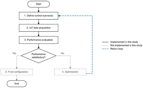
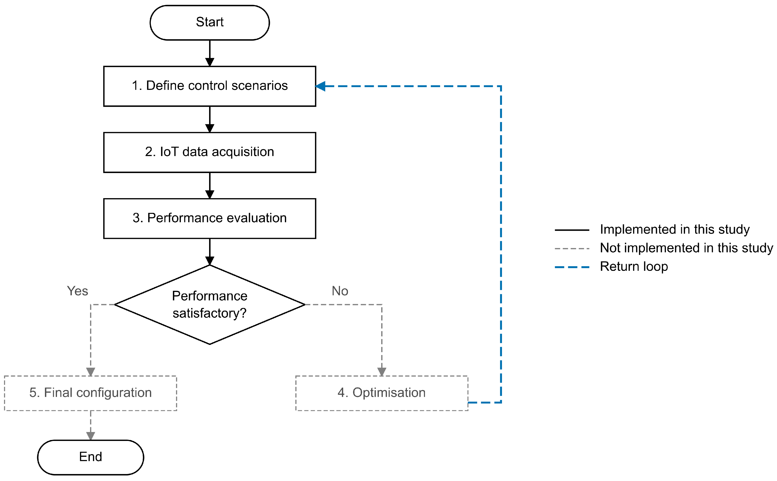
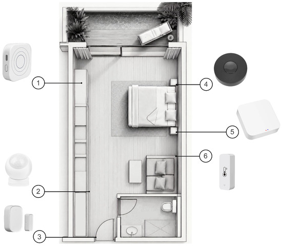
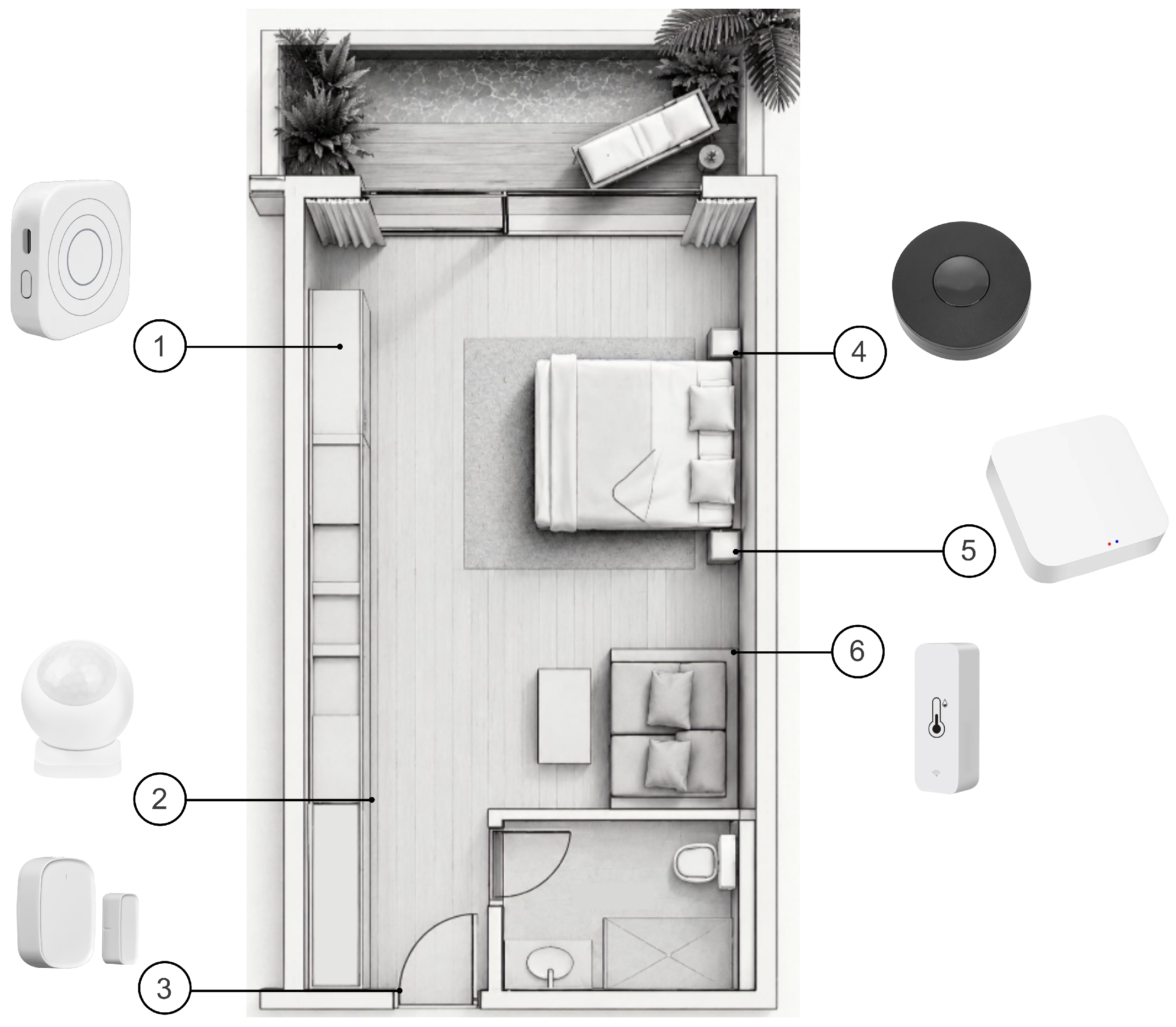
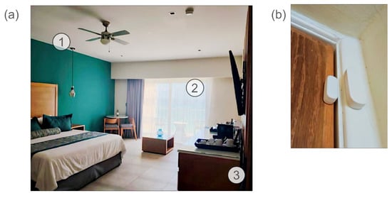
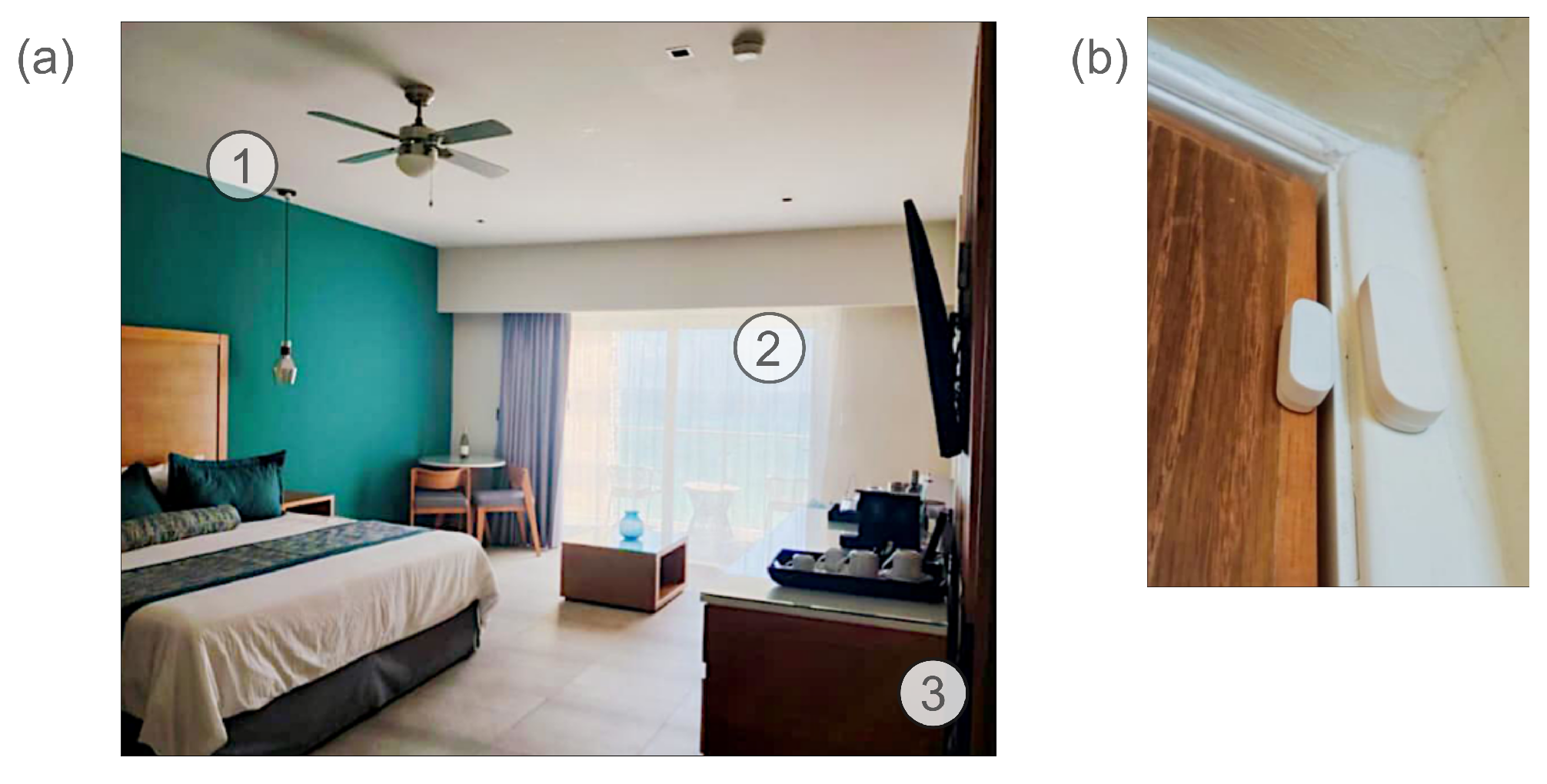
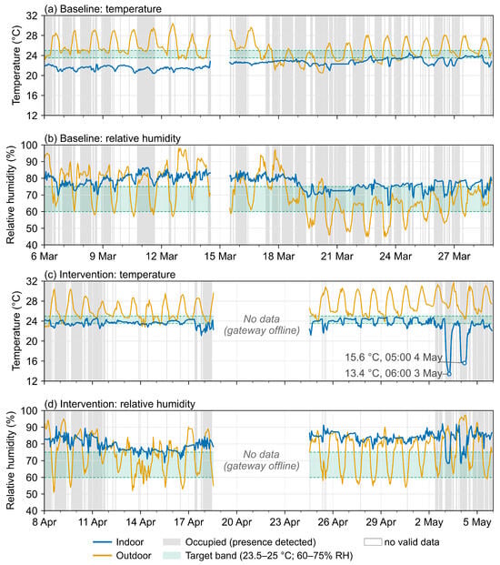
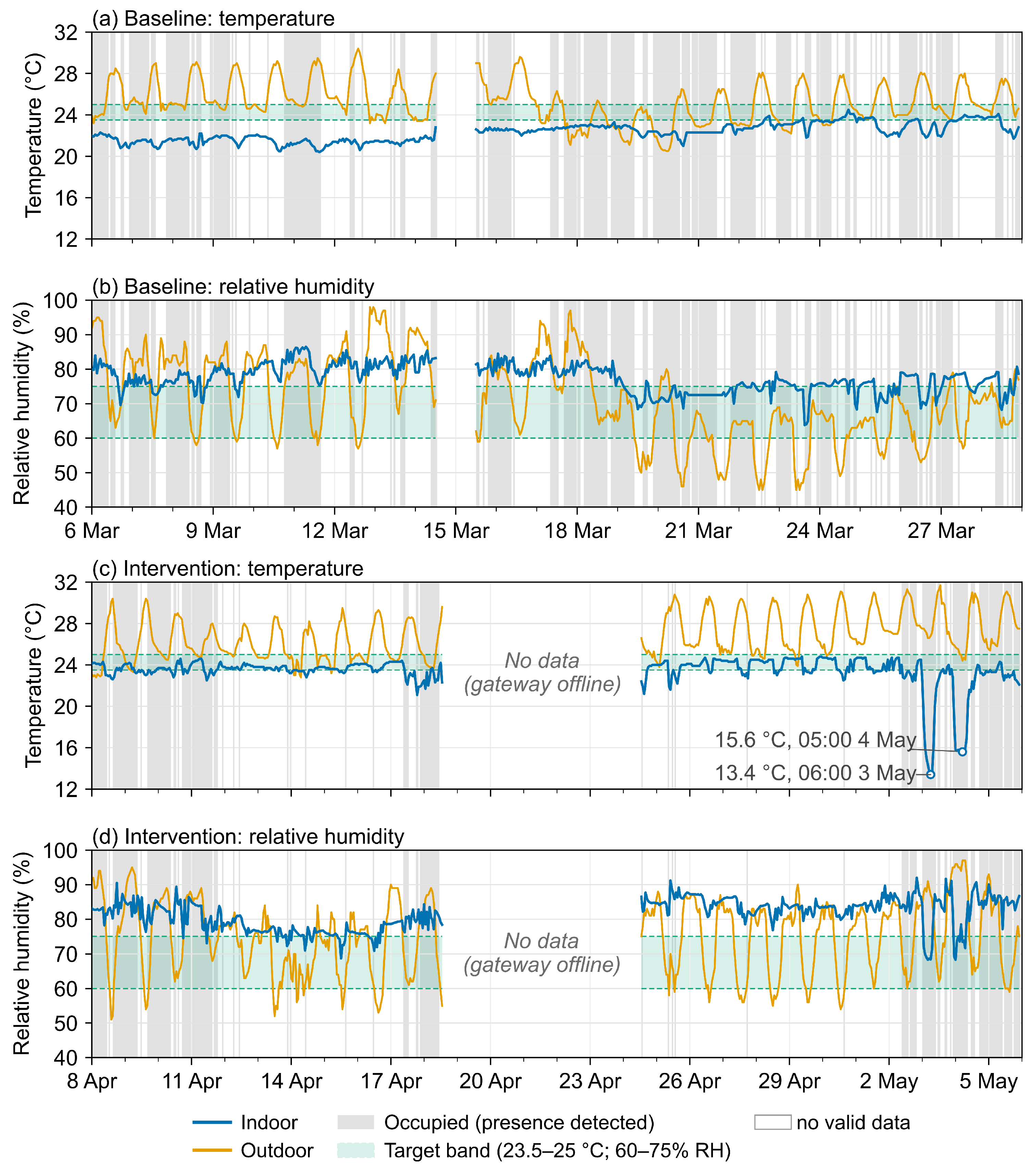
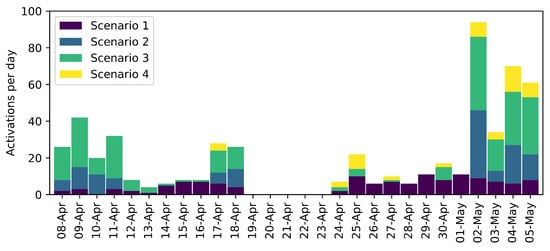
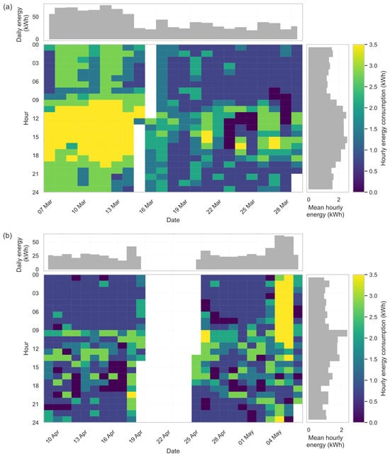

Disclaimer/Publisher’s Note: The statements, opinions and data contained in all publications are solely those of the individual author(s) and contributor(s) and not of MDPI and/or the editor(s). MDPI and/or the editor(s) disclaim responsibility for any injury to people or property resulting from any ideas, methods, instructions or products referred to in the content. |
© 2026 by the authors. Licensee MDPI, Basel, Switzerland. This article is an open access article distributed under the terms and conditions of the Creative Commons Attribution (CC BY) license.