Techno-Economic Assessment of Integrating Renewable Power to Large Inductive Loads Under Power Compensation Schemes: A Case Study of Metropolitan Water Pumping Systems

Abstract

Large inductive loads such as motors and pumps require balanced active and reactive power for their operation. There are two major approaches that are adopted to reduce energy consumption. The capacitor bank scheme (CBS) is mainly used for reactive power compensation, whereas solar power integration (SPI) is used mainly to reduce the burden on the grid while providing active power. However, significant aspects that may need precise quantitative assessment are active power, reactive power, and the power factor variations under the CBS and SPI schemes. This research study proposes an evaluate, quantify, and compare (EQC) framework for CBS and SPI schemes that will help industries to systematically opt for the efficient and cost-effective operation of large inductive loads. Under the EQC framework, detailed quantified trade-offs between active power, reactive power, and power factor corrections were found. It was found that without integrating renewable power, the active power and reactive power on the LV bus were 115 kW and 58.9 kVAR, respectively, compared to CBS, where reactive power was reduced to 34.9 kVAR. SPI approach with unity power factor reduced active power and reactive power to 34 kW and 59 kVAR, respectively. However, the power factor was reduced to 50.4% from 80% in CBS. While integrating solar power with a 90% power factor, the active power was reduced to 34 kW, and the reactive power was reduced to 20 kVAR with the power factor increasing to approx. 90%, proving the suitability of the SPI approach. To further assess the SPI approach in terms of economics, the feasibility analysis for SPI was conducted on HOMER PRO. The NPC reaches up to 1.13 million, which is 30% lower compared to grid supplies. The operation capital cost for solar PV power is USD 63,453. The operational cost is 34% compared to the grid. One of the important parameters is the levelized cost of energy (LCOE). The cost of energy for the grid-based system is set at 0.210 cents, whereas for solar power, the LCOE is set at 0.126 cents, which is 40% less compared to the grid.

1. Introduction

Water-pumping systems are high-power consumption units [1]. Due to their continuous operation, water-pumping systems can be considered high-power consumption units that certainly impact power distribution systems. Due to their higher power consumption, regular energy assessments, formally known as energy audits for pumping stations, are conducted. However, these energy audits have limited boundaries, with most of them limited to the analysis of water being produced against the consumed power [2]. The efficiency of the pumping equipment, including the motor, pump, and connecting shaft, is highly dependent on the proper sizing of all three components [3]. Overall efficiency of the pumping station can be improved by adopting the following measures [4]:

•

Proper sizing of motor and pump;

•

Using an energy-efficient motor;

•

Installing a smart motor control;

•

Improving the low-voltage line.

The cost of electricity is more than 90% of the total operating cost of a municipal water distribution system [4].

In light of the recent literature survey specifically for water-pumping stations, the prime objective of this study is to find energy-saving opportunities while conducting an energy audit of pumping stations. One past work by the Japan International Cooperation Agency (JICA) included an energy savings potential study [1] for the second largest metropolis of Pakistan. The main focus of this project was to identify the pumping stations with less than 95% discharge efficiency and replace the pumping equipment of such stations. One of the major findings of this JICA-led project was the mismatch between the pumping capacity of the centrifugal pump and the output power of the induction motor. However, the study was limited to the assessment of the water pumps themselves. A similar project is described by Miao Qun et al. in [5]. In this project, building information management (BIM) tools were used to design and implement an urban water supply pumping station. The use of BIM greatly improves the environmental impact of a pumping station throughout its life cycle.

Energy efficiency improvements based on water management data and energy recovery were suggested for a water distribution network in South Africa. The study proposed using small-scale hydroelectric turbines to harvest excess energy from pressurized water supply pipes. The results show an annual energy recovery potential of more than 4% for one metropolitan area [6]. Energy efficiency improvements using pump-scheduling optimization were studied in another research work by Tiago Luna et al. The authors proposed a genetic algorithm to develop an optimized hourly pumping schedule based on historical water demand data. The authors modeled the water distribution system and ran simulations using a hydraulic simulation tool. The best-case energy-efficiency results showed a 15% improvement over normal operation [7].

Rudra et al. presented a case study involving water supply systems of multiple cities from Africa [8]. The selected cities had diverse urban settings in terms of population size, altitude, and expansion potential. This study’s findings relate to all three areas: the electrical system, pumping scheme, and distribution network of the water supply infrastructure. The study suggested improvements in all of the above areas. The study suggested voltage regulation and power factor improvements for the electrical system. For mechanical systems, the study suggested replacing multiple smaller pumps with a single high-power pump. At some locations, older inefficient pumps were replaced with newer pumps. The study also suggested updating the piping network to match flow rates between pumps and the water distribution network. A similar study was performed by Fragkoulis Papagiannis et al. to optimize the replacement of aging equipment in the water distribution network of Ukraine. A mathematical technique was proposed to perform multi-factor planning optimization for the replacement of aging pump station equipment [9].

Araceli et al. presented a relationship between the energy consumption and pipe diameter [10] for a water distribution network. For a given water distribution network, especially in urban settings, the demand of water is highly variable. This variable demand challenges designers in choosing an energy-efficient pipe diameter. The presented method can be used to determine an equivalent flow rate, in place of the variable flow rate, to optimize the piping design process from an energy-use perspective. A similar method is presented in [4] for energy assessment of water pumps. Critical operating parameters were recorded from a large number of pumps to arrive at an empirical relationship between the pump efficiency and its flow rate. Both of the above-mentioned methods can be used during the initial design process or after an energy audit to improve the energy efficiency of a water supply system.

A detailed and in-depth study is presented by Kumar et al. in [11]. Energy efficiency data were collected from multiple large cities with specific attention to the water distribution systems. Results of this long study revealed a potential of up to 40% improvement in the energy efficiency of ground water pumping and distribution. A similar comparison is presented by Olivia Jensen et al. to compare the outcome of integrated urban water management schemes of Hong Kong and Singapore. The results clearly show a higher water security index in Singapore after implementing water management processes, due to strong institutionalization and clear objectives [12]. Another interesting study is presented by Farrukh Mahmood and Haider Ali in [13] which compares the energy efficiency of individual water pumping systems with community-level water pumping stations. This study shows that large-scale water pumping is much more efficient, especially when pumping from deep aquifers.

Energy efficiency improvements using a combination of solar energy storage and municipal water storage were proposed by Mario et al. Using the pumped-hydro facility along with an appropriately sized solar farm, the water is pumped to an elevated reservoir during daytime. The stored energy is used during peak hours to minimize fossil fuel use and reduce greenhouse gas emissions. This is especially beneficial for large-scale water distribution networks, where pumping energy requirements are high. Because this hybrid system requires a relatively large water reservoir to store water at elevation, it is only feasible in certain geographic locations [14]. An enhanced version of this approach is presented by S. Liu et al. by simulating a water supply network along with a hybrid energy generation system with multiple energy resources. The proposed simulation model uses pumped-hydro, heat pumps, solar and wind farms, and conventional fossil fuel resources in a hybrid mode. For a thousand-house community, annual heat demands were fulfilled by 63% with a 55% reduction in carbon emissions [15].

A cyber-physical framework is proposed by Congcong Sun et al. to improve the overall efficiency of an urban water management system. A multilayer cyber-physical management system was proposed to control water distribution in a metropolis optimally. The optimization algorithm uses information from multiple subsystems inside a water distribution network, essentially forming a global optimization scheme. The results show that both the sustainability goals and emission targets were met with improved efficiency compared with non-global parameter optimization [9]. Another cyber-physical system is presented by Sanaz Imen et al. to optimize the water treatment process. The proposed system creates a relationship between the water impurities in the source water and treatment plant operating parameters. The required level of water treatment determines the water supply capacity to the distribution network. The proposed algorithm adjusts all of the above parameters in real-time and provides a cyberspace for the decision makers to perform any adjustments if needed [16].

Use of variable speed pumps (VSPs) is discussed by Moustafa Darweesh in [17]. A comparison is presented between fixed speed pumps (FSPs) and VPS. It is observed that the VSP scheme is up to 20% more efficient in terms of electricity usage. Another benefit of VSPs is the reduction in pipe leakages due to lower system pressure. It is evident that energy efficiency and optimization can be fruitful in managing the load effectively [18]. However, the assessment of reactive and active power balance and its impact on power factor under solar power integration varies dynamically, which needs careful attention to achieve optimal power flows [19,20]. Integration of renewable energy into highly inductive loads poses serious challenges to the grid power quality parameters [21]. Inappropriate integration may cause power quality issues where the power factor may significantly reduce under the unbalanced active and reactive power flows, as well as voltage instability in the overall system [22].

Research Gap and Contribution

In recent literature reviews, large inductive loads such as water pumping systems have been assessed in terms of energy efficiency through optimization techniques and energy audit studies in low voltage distribution. When quantified comprehensively, there are interesting trade-offs among active power, reactive power, and power factor, and adjusting them may improve decision-making for industries to optimize power utilization. Solar power integration (SPI) and capacitor bank schemes (CBS) are widely used power-conditioning and optimization approaches, but the trade-offs that severely affect power quality have not been quantified in depth. Moreover, solar power analysis and reactive power compensation schemes are often studied as distinct subjects, even though they are strongly correlated when properly coordinated with power factor adjustments in inverter-interfaced power networks. Studies to quantify reactive power compensation under inverter-interfaced power networks have not been studied in depth.

This research study focuses on developing a complete EQC assessment framework to quantitatively assess reactive and active power balance on the low-voltage side and their impact on power factor when integrating solar power under CBS and SPI schemes. The quantitative analysis highlights the importance of balanced solar power integration and optimized energy use. In the second part of the research, we quantify project economics while integrating solar power to assess the project’s economic suitability. This study contributes to assessing and quantifying power factor adjustments in inverter-interfaced solar power systems and their overall impact on system reactive power compensation. Finally, the manuscript also financially assesses the overall EQC framework for installing a solar PV system over 25 years, providing a techno-economic analysis of large inductive loads such as water pumps in power systems.

2. Materials and Methods

The research is divided into two parts. The first part is a technical assessment of active and reactive power compensation on the low-voltage side, as voltage and power factor vary.

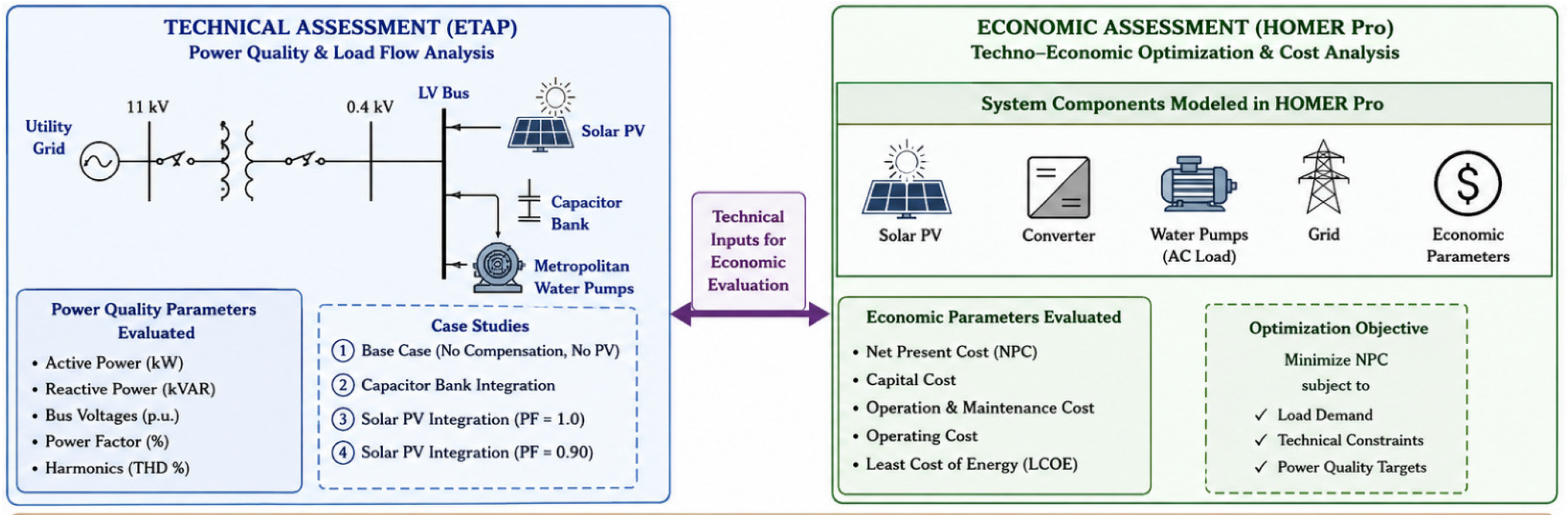
In the second part, the 100 kW solar power integration has been assessed economically using HOMER Pro software. The project’s Net present value, cost of energy, capital and operational cost and payback period have been assessed. The next section provides the details of the technical assessment. Figure 1 shows the techno-economic assessment framework.

Figure 1. Diagnostic and techno-economic assessment framework.

2.1. Technical Assessment

ETAP 20.6.0 software was used for the technical study. In this study, a 100 kW water pumping system that provides water to the metropolitan area was selected.

2.2. System Description and Single-Line Diagram

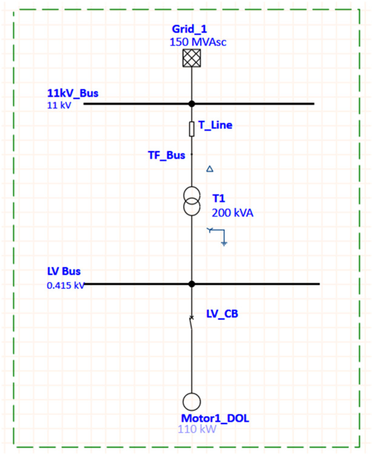
The motor is fed from an 11 kV grid through a 11/0.415 kV step-down transformer. The load is a centrifugal pump, modeled in ETAP using a polynomial torque–speed characteristic. The motor nameplate and system parameters used throughout the simulation are summarized in Table 1, Table 2, Table 3 and Table 4 below.

Table 1. Grid source data.

Grid Parameter	Value
System	150 MVAsc
Nominal Voltage	11 kV

Table 2. Motor and system data.

Motor Parameter	Value
Designation	Induction Motor
Rated Power	150 HP (110 kW)
Rated Voltage	0.415 kV
Rated Speed	3000 RPM
Poles	2
Nameplate Power Factor	89% at FL
Motor Efficiency	95.6% at FL
Starting Method	Direct-On-Line (DOL)
Connected Bus	LV Bus

Table 3. Transformer Data.

Transformer Parameter	Value
Designation	2-Winding Transformer (T1)
Rating	200 kVA
Voltage	11 kV/0.415 kV
Vector Group	Dyn11
Impedance (%Z)	4.0%
X/R Ratio	1.5

Table 4. Transmission Line Data.

Transmission Line Parameter	Value
Length	3.0 km
Conductor	BOWLS 1120
Conductor Size	120 mm2
Nominal Voltage	11 kV

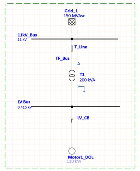
The network single line diagram is shown in Figure 2. The topology of the grid, a 200 kVA step-down transformer, LV bus, and motor/pump, is the same for the three starting cases considered in this study; only the starting device connected to the motor terminals changes between the DOL, VFD, and autotransformer simulations.

Figure 2. System single-line diagram.

2.3. Load Flow Analysis

A load flow analysis was carried out to evaluate the motor’s steady-state conditions in the system. The load flow uses different case scenarios to observe the motor’s impact on the HV and LV bus voltages, power factor (PF), and harmonics in the system. Equations (1)–(4) below are used to evaluate the harmonic distortion, power quality, and the PF correction [23].

2.4. Harmonic Distortion

The standard equations used for the total harmonic distortion (voltages) to figure out the results are given in Equation (1) below:

$$\mathit{TH}{D}_V\left(\%\right)={\displaystyle \frac{\sqrt{{\sum }_{h=2}^{h_{\mathit{max}}}{\left(V_h\right)}^2}}{V_1}}\times 100$$

(1)

The equation shows the combined magnitude of all the harmonic voltage components as a percentage of the fundamental voltage and is the quantity compared directly against the IEEE 519 Standard limit [24]. The single harmonic order Equation (2) is given below.

$${\mathit{IHD}}_h\left(\%\right)=\left({\displaystyle \frac{V_h}{V_1}}\right)\times 100$$

(2)

2.5. Power Factor

Equation (3) shows the standard relationship between real power (P), reactive power (Q), and the resulting power factor, and this report uses it to quantify the power factor at each bus in each case.

$$\mathit{PF}=\mathit{cos}\left(\theta \right)={\displaystyle \frac{P}{\sqrt{\left(P^2+Q^2\right)}}}$$

(3)

2.6. Capacitor Bank Sizing

When the system power factor, calculated by Equation (3), falls below the standard limits the PF correction becomes important. One solution to this suboptimal operation is to install capacitor banks at specific buses, called target buses. The theoretical reactive power capacity Qc required for the correction of low power factor is calculated by using Equation (4) as the difference between the uncorrected phase angle tan θ₁ and the improved phase angle tan θ₂.

Qc = P × (tan θ₁ − tan θ₂)

(4)

In this study, the mathematical calculation resulted in a reactive power compensation requirement of approximately 20 kVAR. A 25 kVAR capacitor bank is chosen for the ETAP assessment to achieve the desired power factor correction under the modeled operating conditions. A 20 kVAR option is very close to the theoretical minimum, and 30 kVAR banks would overcompensate, increasing the risk of overcompensation under light-loading conditions. The 25 kVAR selection gave a power factor of approximately 0.957 on the LV bus under the simulated condition. This approach provides the reactive power needed to optimize system voltages and PF without overcorrecting the grid network.

2.7. Motor Starting Analysis

The motor starting analysis was carried out to assess the transient conditions on the system. To observe the pump controlling techniques, three different starting conditions were used for motor starting analysis including DOL, VFD and the autotransformer operation, which were tested in ETAP to evaluate the voltage, current behavior and the torque of motor during the start based on the induction motor equivalent model and the starting conditions [25].

The fundamental premise is the standard per-phase equivalent-circuit expression of induction motor torque as a function of slip, described in Equation (5):

$$T={\displaystyle \frac{3V^2(R2/s)}{\left\{\omega s\right[(R1+R2/s)2+(X1+X2)2\left]\right\}}}$$

(5)

In the equation above, V is the stator phase voltage, R1 and R2 are the stator resistance and X1 and X2 are the stator reactance, s is the slip and ws the synchronous speed. In Equation (5), torque is at a constant slip and frequency is proportional to the square of the voltage applied. This voltage–torque scaling in Equation (6) is the relation that governs both DOL and autotransformer motor starting:

$$(T\propto V^2)\Rightarrow {\displaystyle \frac{T_2}{T_1}}=({{\displaystyle \frac{V_2}{V_1}})}^2$$

(6)

The application of Equation (6) includes both DOL and autotransformer starts. DOL (direct-on-line) starting is a full-voltage starting in which the motor is connected across the line at the rated voltage without any current limiting device. For an autotransformer starter with tap ratio a (0 < a < 1), the motor side voltage and current quantities are specified in Equations (7) and (8):

V_MOTOR = a.V_line, I_MOTOR = a.I_LR

(7)

T_Start = a².T_DOL, I_line = a².I_LR

(8)

The source current decays faster with the ‘a²’ than the motor side current, which decays only with the ‘a’. This ‘a²’ reduction is the key advantage of the autotransformer over the series impedance starter.

Unlike the DOL and autotransformer starter, the VFD does not rely on Equation (6). Instead, it uses Volts/Hertz control, defined in Equation (9) below:

$${\displaystyle \frac{V}{f}}={\displaystyle \frac{V_{\mathit{rated}}}{f_{\mathit{rated}}}}=\mathit{constant}\Rightarrow \Phi =\mathit{constant}$$

(9)

As the air-gap flux Φ is held constant during the ramp, the VFD starting current is set directly by a closed loop current limit control (typically 1.0–1.5 × FLA) and is not governed by Equation (2); this explains why VFD current does not follow the V² condition while governing DOL and the autotransformer starting.

The behavior of the VFD current limiting model is expressed in Equation (10) below:

$$\mathit{Is}\left(t\right)=\mathit{min}\left[V_{{\displaystyle \frac{v}{f}}}\right(t),I_{\mathit{Limit}}]$$

(10)

where:

I_Limit = k ⋅ I_FLA (k ∈ [1.0, 1.5])

The $V_{{\displaystyle \frac{v}{f}}}\left(t\right)$ Vv(t)/f is the current that would be obtained from the open V/f ramp, and I_Limit is the limit of the current setpoint. When $V_{{\displaystyle \frac{v}{f}}}\left(t\right)$ exceeds I_Limit, as occurs near breakaway, the pump’s static torque A₀ = 10%, as shown in Equation (8). The controller still has to be overcome; the frequency ramp is decreased instead of allowing current to increase according to V². This is why the VFD’s start time is longer than the DOL’s, as the performance metrics in the results section show.

The mechanical load the motor must accelerate against is the pump’s torque–speed characteristic used within ETAP, given by the polynomial curve fit in Equation (11):

T_load = A₀ + A₁ω + A₂ω² + A₃ω³

(11)

where A₀ = 10, A₁ = –91, A₂ = 321, A₃ = –147, and ω is the per unit speed (0 to 1), taken from the standard pump load model of ETAP. A₀ = 10% is the pump breakaway torque at zero speed (static head and friction).

2.8. Economic Analysis

As analyzed in the previous section, integrating renewable power for power-quality analysis is well suited to large inductive loads once the parameters are properly tuned. In this section, to analyze the economic impact of integrating renewable power, metrics such as net present cost, cost of energy, payback period, and capital cost of integrating renewable power are calculated. HOMER Pro software was used for the economic analysis. The major economic parameters that directly impact project costs are capital and operational costs. The capital cost can be expressed as given in Equation (12), whereas the cost of energy can be expressed as given in Equation (13) [26].

$$C_{\mathit{capital}}={\displaystyle {\sum }_{j=1}^n}{C}_{\mathit{capital}j}$$

(12)

$$\mathit{COE}={\displaystyle \frac{C_{\mathit{ann},\mathit{tot}}}{E_{\mathit{served}}}}$$

(13)

where:

•

COE = cost of energy (USD/kWh);

•

Cann,tot = total annualized cost (USD/yr);

•

Eserved = annual electrical energy served (kWh/yr).

The per-kW cost of solar power was set at USD 375, whereas the operational cost was set at USD 10 per kW. The derating factor for solar power was kept at 80%. For the grid side, the per-unit cost was set at USD 0.210 and energy selling price was kept at USD 0.10.

Other than capital and operational cost, the decisive parameter for integrating renewable power economically is net present cost, which helps to evaluate the project cost over a 25-year period span; this can be expressed as Equation (14).

$$\mathit{NPC}=C_{\mathit{ann},\mathit{tot}}{\displaystyle \frac{{(1+i)}^N-1}{{i(1+i)}^N}}$$

(14)

where:

• NPC = total net present cost;
• Cann,tot = total annualized cost;
• i = annual real interest rate;
• N = project lifetime in years.

As pumping stations operate mainly twice a day, a 100 kW pump load profile was used. Due to two major peaks, the load factor was 0.5, and the average load was 49 kW, which is less than 50% of the peak load of 100 kW. Table 5 below shows the system sizing.

Table 5. System configuration and sizing.

Component	Name	Size	Unit
PV	Generic flat plate PV	100	kW
System converter	System Converter	86.5	kW
Grid	Grid	unlimited	kW

2.9. Power Sell Back to Grid

HOMER Pro uses instantaneous power flow to determine the grid sales. The software accumulates the power that is sold back or exported over the simulation steps based on the designated time steps to obtain the energy sold in kWh.

The power that is sold back to the grid is calculated as given in Equation (15):

P_grid = P_generation − P_load − P_{batterycharging}

(15)

The power to be sold can be calculated as given in Equation (16):

P_sale = max(0,P_grid)

(16)

The solar energy can be calculated as given in Equation (17):

E_sale,t = P_sale,t×∆t

(17)

The overall Egrid sales can finally be calculated as given in Equation (18).

$$E_{\mathit{grid}\mathit{sales}}={\displaystyle \sum _{t=1}^N}{P}_{\mathit{sale},t}∆t$$

(18)

where:

• Psale, t = power exported to grid at time t (kW);
• ∆t = simulation time step (h);
• E_grid sales = total energy sold to grid (kW).

2.10. PV Sizing

The PV size is deliberately below the motor nameplate rating (110 kW) to avoid extra capital expenditure while still providing substantial power generation. The selected solar system also allows analysis of the impact on the grid, while the grid seamlessly supplies the remaining power during peak demand. The motor’s actual operational demand varies below its nameplate rating due to the conventional design safety margins. However, to maintain conservative margins, the steady-state load flow assumes the motor operates at 100% capacity to evaluate system conditions.

3. Results

3.1. Load Flow Analysis Results:

3.1.1. Case 1: Baseline Case with No Compensation

In this case, the motor is tested direct-on-line with no reactive power compensation and an independent generation source at the LV Bus.

The simulation results are provided in Table 6. The load flow results show that the power factor of all three buses is around 89%. The total voltage drop across the system is 2.48%, which is due to the impedance of the 3 km transmission line and the transformer carrying the motor’s full operational current.

Table 6. Baseline Case 1 results.

Bus	Nominal Voltage (kV)	Operating Voltage (kV)	Operating Voltage (%)	Current (A)	Power (kW)	Power (kVAR)	PF (%)	THDV (%)
11 kV Bus	11	11	100.00	6.9	117.1	60.7	88.8	0.17
TF Bus	11	10.982	99.84	6.9	117.1	60.7	88.4	0.17
LV Bus	0.415	0.405	97.52	184.3	115	58.9	89.0	0.15

3.1.2. Case 2: Capacitor Bank Compensation

In this case, a 25 kVAR capacitor bank is connected to the LV Bus; the capacitor is sized according to Equation (4) to raise the PF from 89% toward a target of 95%. This represents the conventional, lowest-capital-cost approach to power factor correction at a load of this size.

The installation of the 25 kVAR capacitor bank brings the PF of all buses up to 95.5%, as shown in Table 7. This reactive support decreases the motor bus current from 184.3 A to 170.7 A, which results in a decrease in line losses and also helps increase the terminal voltage up to 97.96%. Overall harmonics remain within the safe limit of 5.0% specified by the IEEE 519 Standard. Still, the new capacitor-network impedance focuses the background distortion on the 11th harmonic order and doubles the transformer harmonic current. This resonance change is currently compliant and within limits but may need close monitoring in the event of future expansion.

Table 7. Case 2: results with capacitor bank compensation.

Bus	Nominal Voltage (kV)	Operating Voltage (kV)	Operating Voltage (%)	Current (A)	Power (kW)	Power (kVAR)	PF (%)	THDV (%)
11 kV Bus	11	11	100.00	6.4	116.8	36.2	95.5	0.16
TF Bus	11	10.98	99.87	6.4	116.8	36.2	95.2	0.16
LV Bus	0.415	0.407	97.96	170.7	115	34.9	95.7	0.15

3.1.3. Case 3: Renewable Energy Integration

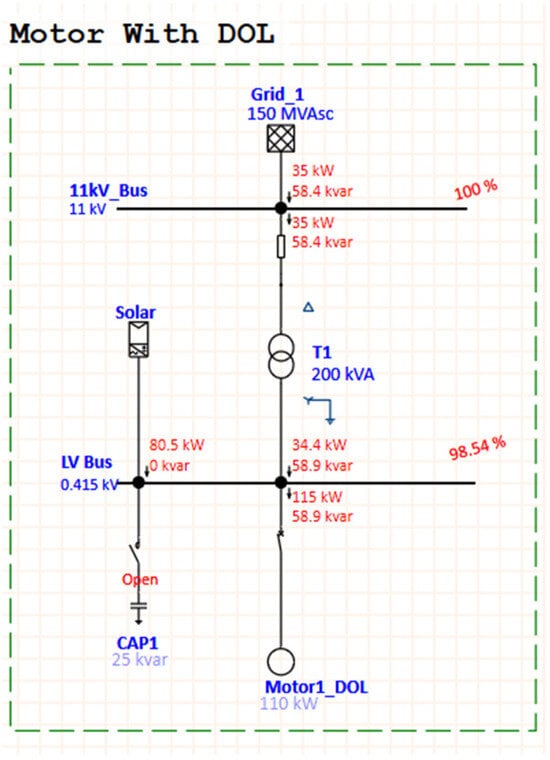
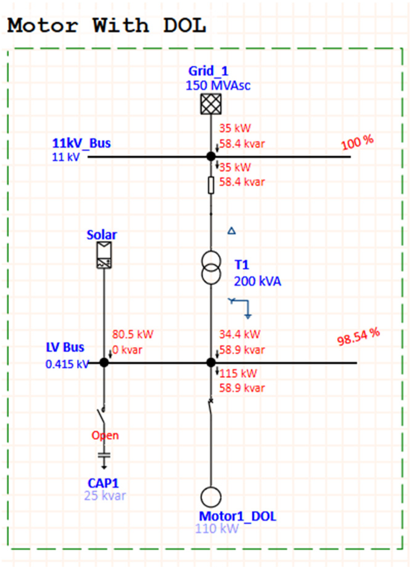
For this case, a 100 kW solar PV source is connected at the LV Bus as shown in Figure 3, sized intentionally below the motor’s real power demand. This means the PV source will never export power back through this transformer, and a comparison is drawn between two different inverter modes of operation: Case 3A, where the inverter operates at 100% power factor supplying only real power, and Case 3B, where the inverter is operated with partial reactive support with a power factor of about 90%. In comparison, the effect of the inverter’s reactive power setting on its real power is offset by the effect of the real-power offset itself.

Figure 3. Case 3A: load flow SLD with PV inverter at 100% PF.

• Solar PV with 100% PF:

In this configuration (Figure 4), the inverter supplies 80.5 kW of real power and no reactive power compensation since the inverter is operating at unity PF. The results are summarized in Table 8 below:

Table 8. Case 3A: results with PV inverter at 100% PF.

Bus	Nominal Voltage (kV)	Operating Voltage (kV)	Operating Voltage (%)	Current (A)	Power (kW)	Power (kVAR)	PF (%)	THDV (%)
11 kV Bus	11	11.000	100.00	3.6	35	58	51.4	0.09
TF Bus	11	10.991	99.92	3.6	35	60	50.6	0.09
LV Bus	0.415	0.409	98.54	96.3	34	59	50.5	0.08

Since the solar inverter only injects real power at a unity power factor, the grid must continue to supply the entire inductive reactive power demand of the motor. This large reduction in grid active power, combined with the constant reactive load, results in a heavy deterioration of the active-to-reactive ratio. The measured displacement power factor at grid connection point collapses to around 51%. This drop is a well-known network phenomenon of real-power solar offset. Although the overall apparent power and line current decrease, the displacement power factor deteriorates because the fixed reactive component dominates the smaller total power vector.

The intermittent nature of solar generation does not affect continuous operation because the PV system is integrated in a grid-connected configuration rather than operating as an isolated source. The 11 kV utility connection acts as an instantaneous balancing mechanism. If PV generation drops, the grid supplies the additional power required.

2.

Solar PV with 90% inverter power factor:

Figure 4. Case 3B: load flow SLD with PV inverter at 90% PF.

Figure 4. Case 3B: load flow SLD with PV inverter at 90% PF.

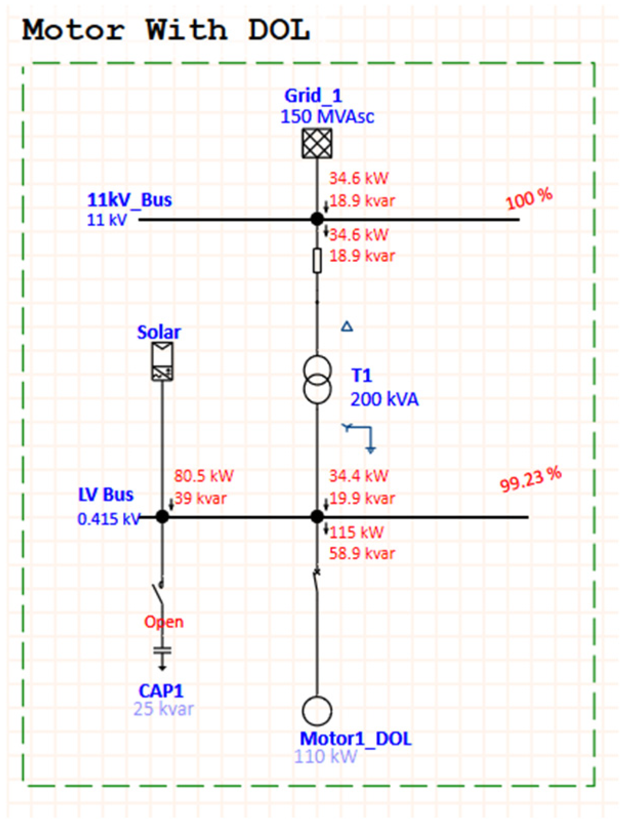
In this configuration, the inverter delivers approximately 81 kW of real power and 39 kVAR of reactive power, with an operating power factor of approximately 90%. The results are summarized in Table 9 below:

Table 9. Case 3B: results with inverter PF 90%.

Bus	Nominal Voltage (kV)	Operating Voltage (kV)	Operating Voltage (%)	Current (A)	Power (kW)	Power (kVAR)	PF (%)	THDV (%)
11 kV Bus	11	11.000	100.00	2.1	35	19	87.8	0.05
TF Bus	11	10.995	99.95	2.1	35	20	86.4	0.05
LV Bus	0.415	0.412	99.23	55.8	34	20	89.0	0.04

In addition to real power, the inverter now provides partial reactive support, reducing the grid’s required reactive power from 60.7 kVAR at baseline to 19 kVAR. The grid-side power factor recovers to 87.8%, close to the baseline level and much better than Case 3 with the inverter PF at unity. The best voltage result among the four cases is achieved by reducing the real and reactive current through the line and transformer. The LV bus voltage increases to 99.23%, which corresponds to a voltage drop of only 0.77%.

A sudden motor trip is simulated in ETAP. The resulting LV voltage increased to approximately 101% (0.419 kV), which is still within the normal inverter operating range. However, in this study, reverse-power protection at the point of common coupling is not implemented; this means that, at sudden load rejection, the PV exports power to the grid. Therefore, the present simulations cannot conclusively assess inverter tripping during sudden load rejection; further studies should verify this through a dedicated protection analysis.

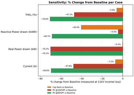
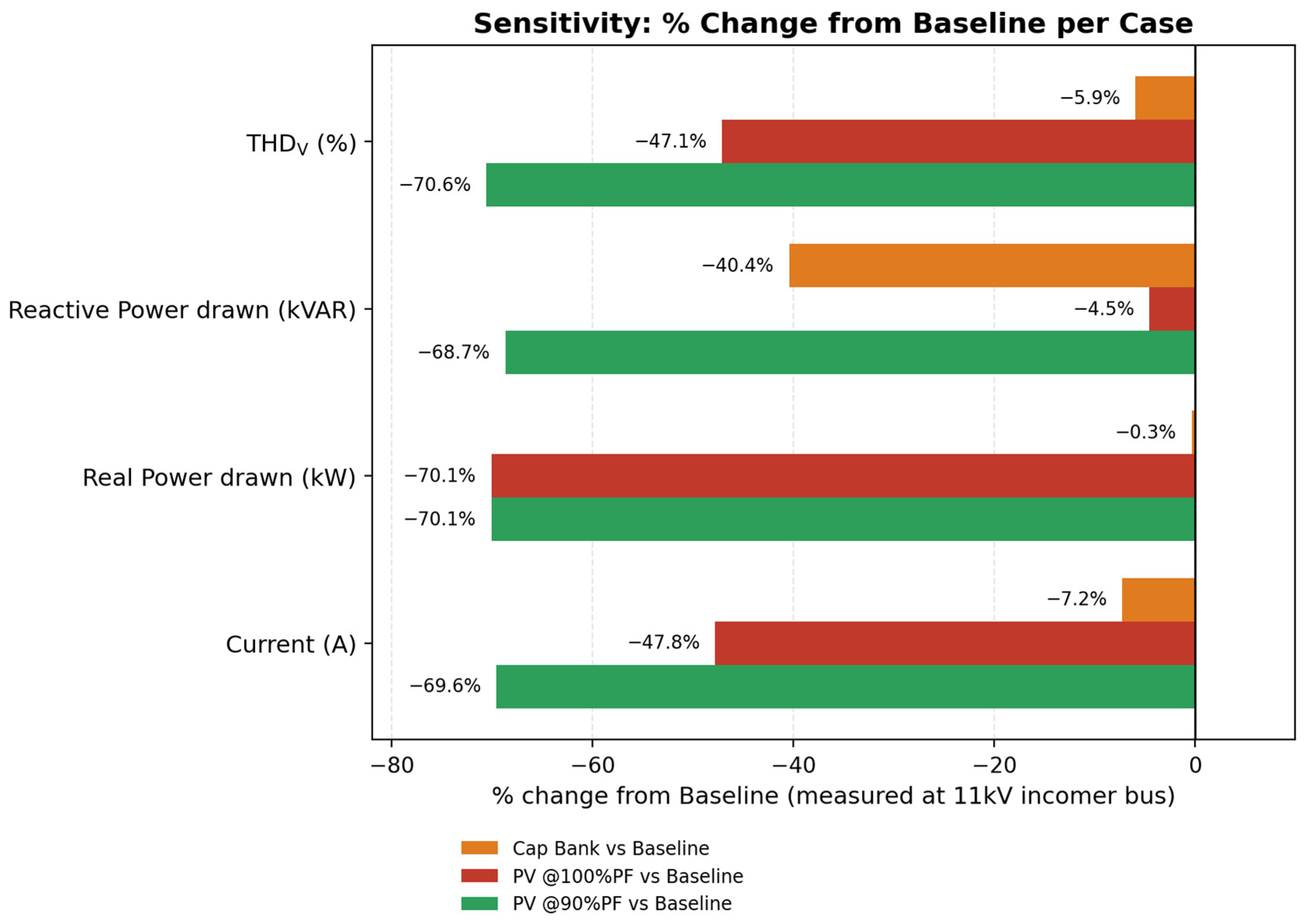
Figure 5 shows the sensitivity analysis comparing the percentage change from baseline for three cases of the ETAP study: capacitor bank case, PV inverter at 100% PF, and PV inverter at 90% PF; and four parameters measured at the 11 kV incomer bus: real power, reactive power, current, and voltage THD. The resulting plot indicates that the injection of the PV inverter at 90% power factor produces the highest improvement and results in a large reduction in almost all of the parameters due to both active and reactive power support that the inverter provides.

Figure 5. Percentage change in each case comparing to baseline case.

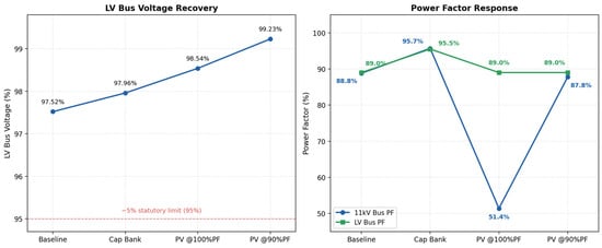
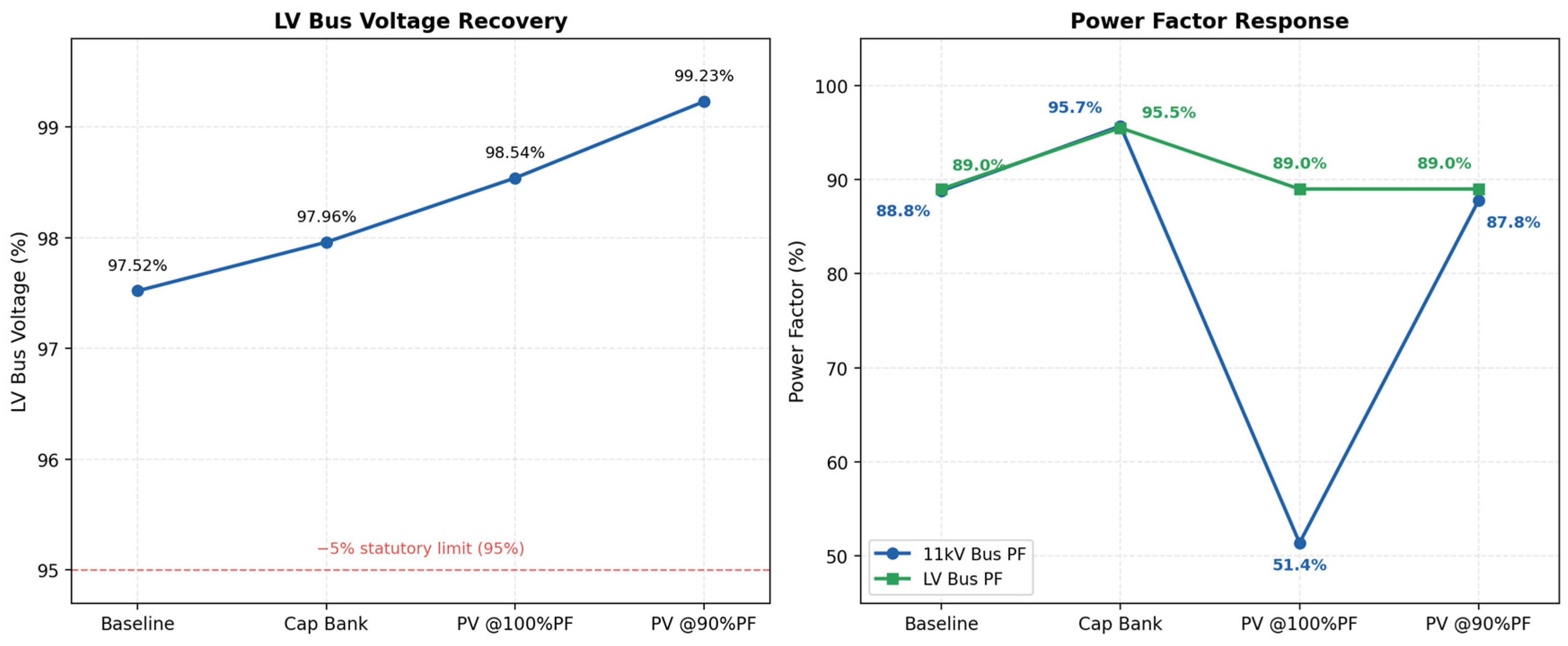
Figure 6 shows the impact on voltage and power factor performance trends in all operating scenarios. Bus voltages significantly improve in each case with the addition of each support, from 97.52% in the baseline case to 99.23% with the PV inverter at 90% PF. All the voltage levels are within the ±5% range. The system power factor in the baseline case is about 89%. However, when the inverter operates at unity PF, the grid power factor drops to 51.4% because the active power contribution comes only from the inverter; it does not contribute any reactive power to the grid. Real power consumption from the grid significantly reduces, while reactive power demand remains the same. When the inverter PF was set to 90%, the grid power factor returned to 87.8% due to reactive power compensation, which is very close to the LV bus power factor of 89.0%.

Figure 6. Impact on voltage and power factor in each case.

3.2. Motor Starting Analysis Results

The motor starting analysis is used to evaluate the effect of three starting methods: direct-on-line (DOL), variable frequency drive (VFD), and autotransformer starter on starting current, input-bus voltage dip, and accelerating torque for a 150 HP, 0.415 kV induction motor driving a centrifugal water pump. ETAP was used for motor acceleration simulations with the same grid/transformer configuration, the only change being the starting device at the motor terminals.

The starting performances of the three methods obtained from the ETAP motor-acceleration simulations are compared in Table 10.

Table 10. Performance comparison of motor starting analysis.

Parameter	DOL (Direct-on-Line)	VFD (V/f Ramp)	Autotransformer Starter
Rated FLA	179.5 A	179.5 A	179.5 A
Peak starting current	600% FLA	150% FLA	450% FLA
Bus Voltage—Maximum	97.52%	98.8%	97.52%
Bus Voltage—Minimum	85%	97.5%	90%
Peak acceleration torque	250 to 300%	70 to 100%	140%
Approx. time to rated speed	3 s	3 s	4 s

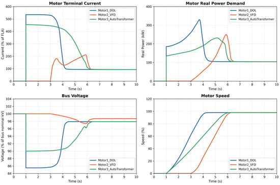
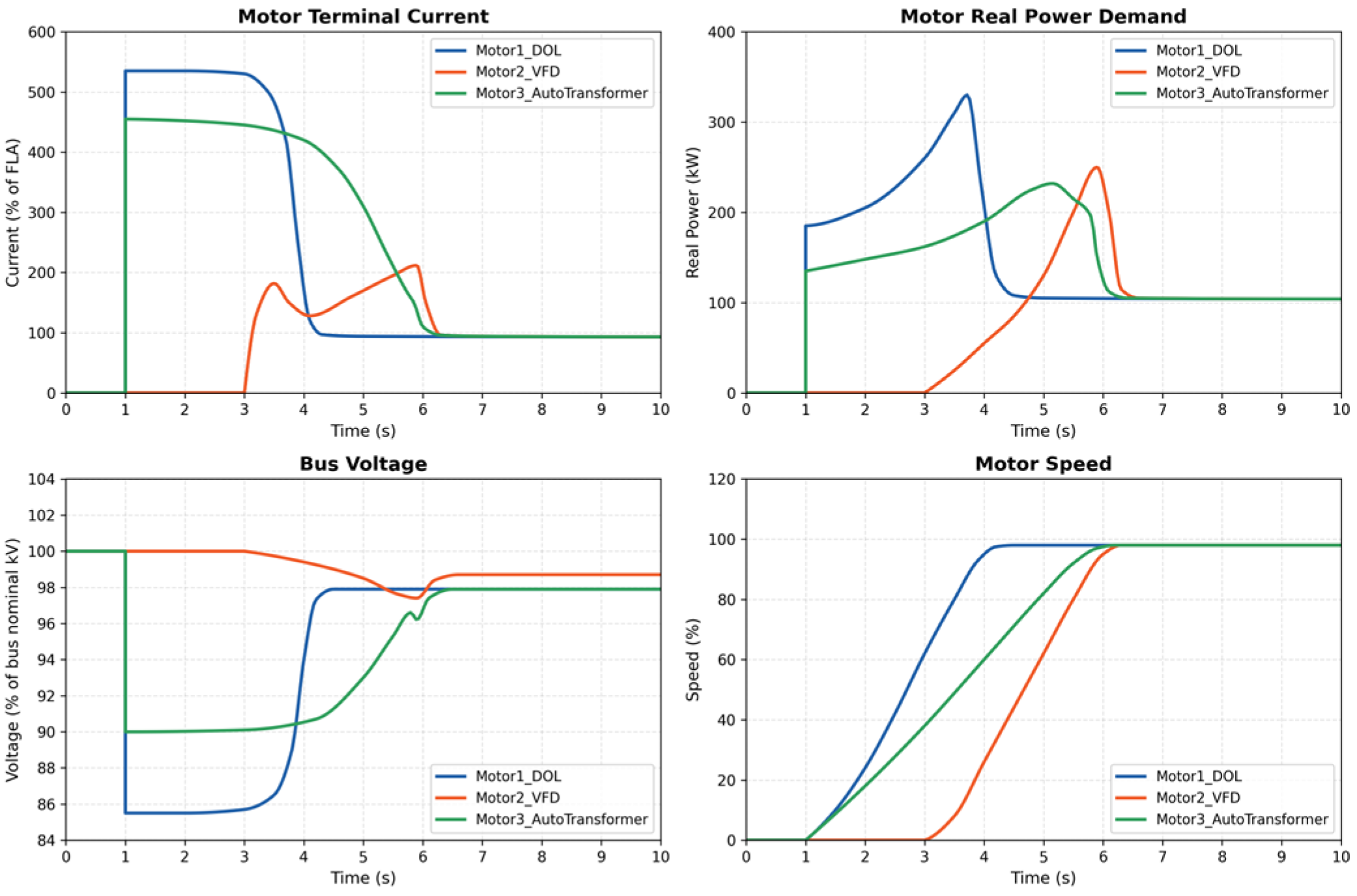
The motor starting behavior of the three methods is shown in Figure 7 below, where Motor1 is DOL starting, Motor2 is VFD starting, and Motor3 is autotransformer starting. DOL has the largest inrush current and the largest voltage drop, but the fastest time to rated speed. The autotransformer is used to minimize inrush current and voltage dip by changing the tap. The VFD produces the smoothest ramp with the least disturbance to the bus voltage and current, but has a longer start time.

Figure 7. Results of motor starting analysis.

3.3. Economic Analysis

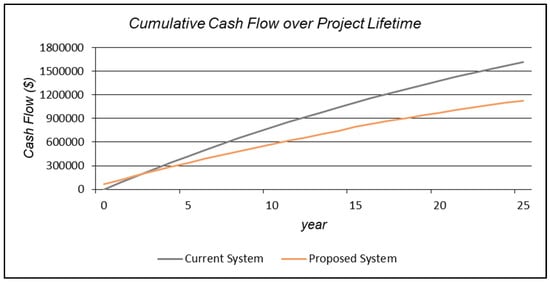
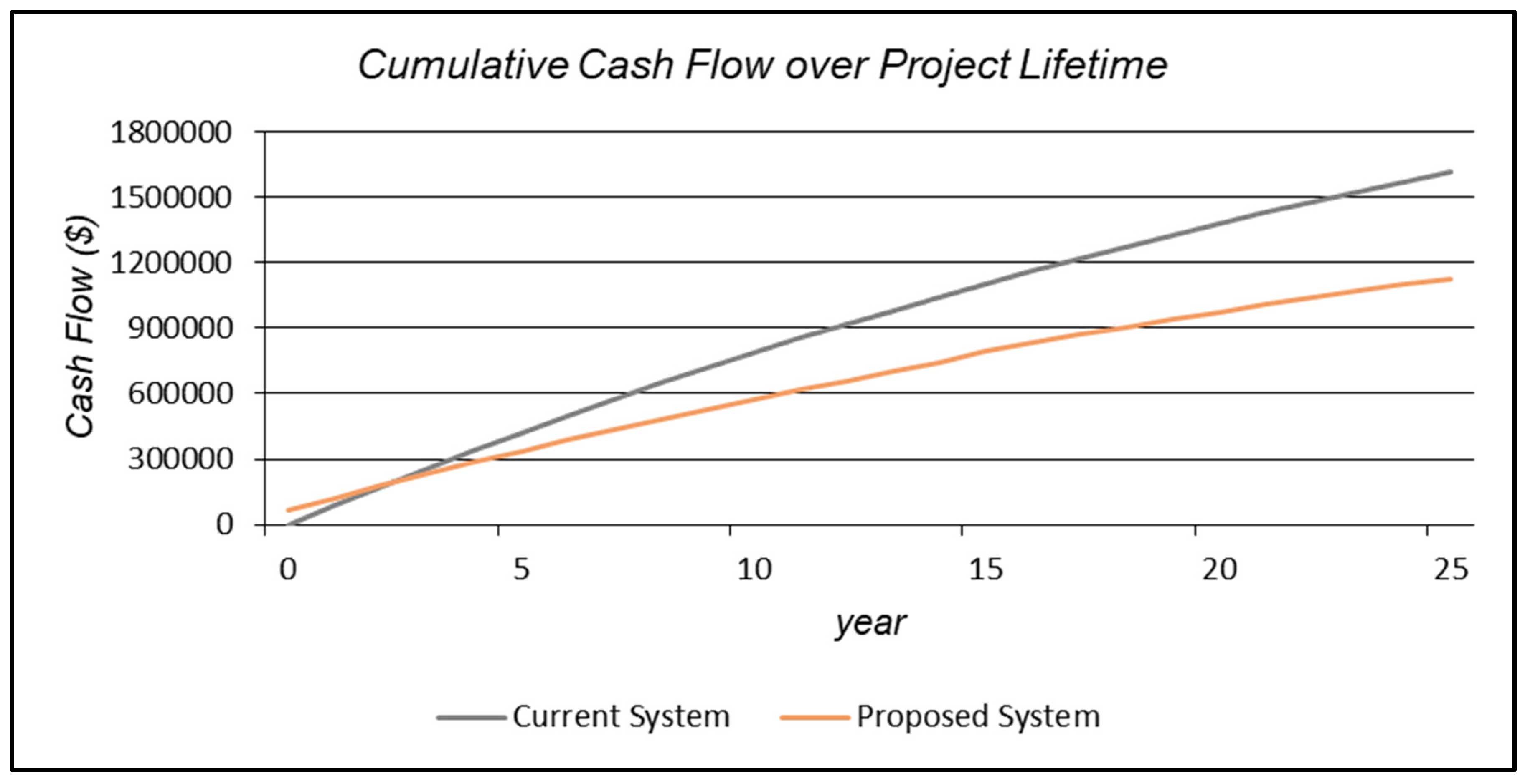
While integrating 100 kW solar power into the existing grid, encouraging results were achieved. Although solar worked only during the daytime, the total capital cost of the system was USD 63,453, whereas the payback period was approx. 2 years (Figure 8) with the net present cost of USD 491,968. Table 11 below shows the return on investment that was 45.5% and annualized savings of USD 31,391.

Figure 8. Cash flow comparison of the systems.

Table 11. Financial and economic analysis.

Parameter	Value
Simple payback:	1.98 yr
Return on Investment:	45.5%
Internal Rate of Return:	50.6%
Net Present Value:	USD 491,968
Capital Investment:	USD 63,453
Annualized Savings:	USD 31,391

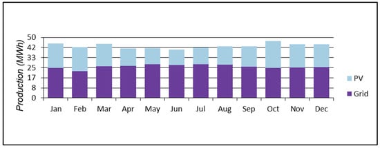
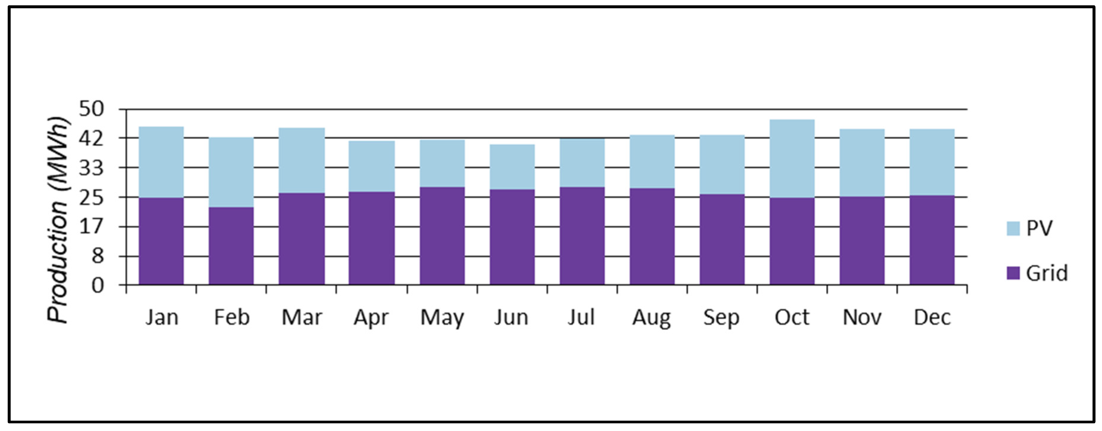
This microgrid requires 1339 kWh/day and has a peak of 100 kW. In the proposed system, the following generation sources serve the electrical load. In Figure 9, it can be seen that utilization of the grid was reduced to half, where the total energy purchases reached an annual reading of 310,333 kWh, as shown in Table 12. The highest months for energy purchases from the grid were in summer, from May to August, which is rational as water utilization increases during the summer. The total energy sold was 68,255 kWh, which contributes to lowering the overall project cost and payback period.

Figure 9. Monthly energy production from PV and grid.

Table 12. Monthly energy billing summary.

Month	Energy Purchased (kWh)	Energy Sold (kWh)	Net Energy Purchased (kWh)	Peak Demand (kW)	Energy Charge	Demand Charge
January	24,928	7629	17,299	100	USD 4472	USD 0.00
February	22,035	7340	14,695	100	USD 3893	USD 0.00
March	26,122	6294	19,828	100	USD 4856	USD 0.00
April	26,344	4328	22,015	100	USD 5099	USD 0.00
May	27,689	3511	24,179	99.8	USD 5464	USD 0.00
June	27,072	3365	23,708	99.5	USD 5349	USD 0.00
July	27,777	3654	24,123	99.4	USD 5468	USD 0.00
August	27,645	4615	23,030	100	USD 5344	USD 0.00
September	25,677	5680	19,997	100	USD 4824	USD 0.00
October	24,766	8000	16,766	100	USD 4401	USD 0.00
November	25,005	7028	17,977	100	USD 4548	USD 0.00
December	25,274	6812	18,461	100	USD 4626	USD 0.00
Annual	310,333	68,255	242,078	100	USD 58,344	USD 0.00

Comparing the grid-only system and solar integrated system, Table 13 shows that the NPC of the grid-only system reached 1.62 million, whereas when integrating the solar PV, the NPC reaches 1.13 million, which is 30% lower and clearly shows that integrating solar PV power with metropolitan pumps is highly favorable. The operation capital cost for solar PV power is USD 63,453 and 0 for the grid, as the grid is already operational. The operational cost of the grid is USD 91,455, whereas for solar power integration, the operational cost is USD 60,064, which is 34% lower compared to the grid. One important parameter is the levelized cost of energy (LCOE). The cost of energy for the grid-based system is set at 0.210 cents, whereas for solar power, the LCOE is set at 0.126 cents, which is 40% less compared to the grid.

Table 13. Cost and emission comparison of both systems.

	Base System	Proposed System
Net Present Cost	USD 1.62M	USD 1.13M
CAPEX	USD 0.00	USD 63,453
OPEX	USD 91,455	USD 60,064
LCOE (per kWh)	USD 0.210	USD 0.126
CO2 Emitted (kg/yr)	275,236	152,993

While discussing the statistics of solar PV, Table 14 shows that the rated capacity of solar PV is 100 kW, with a mean output of 23.4 kW and a capacity factor of 23.4, since the mean energy output per day is 562 kWh/d. Total production was 205,129 kWh/yr.

Table 14. PV array parameters.

Quantity	Value	Units
Rated Capacity	100	kW
Mean Output	23.4	kW
Mean Output	562	kWh/d
Capacity Factor	23.4	%
Total Production	205,129	kWh/yr

4. Sensitivity Analysis

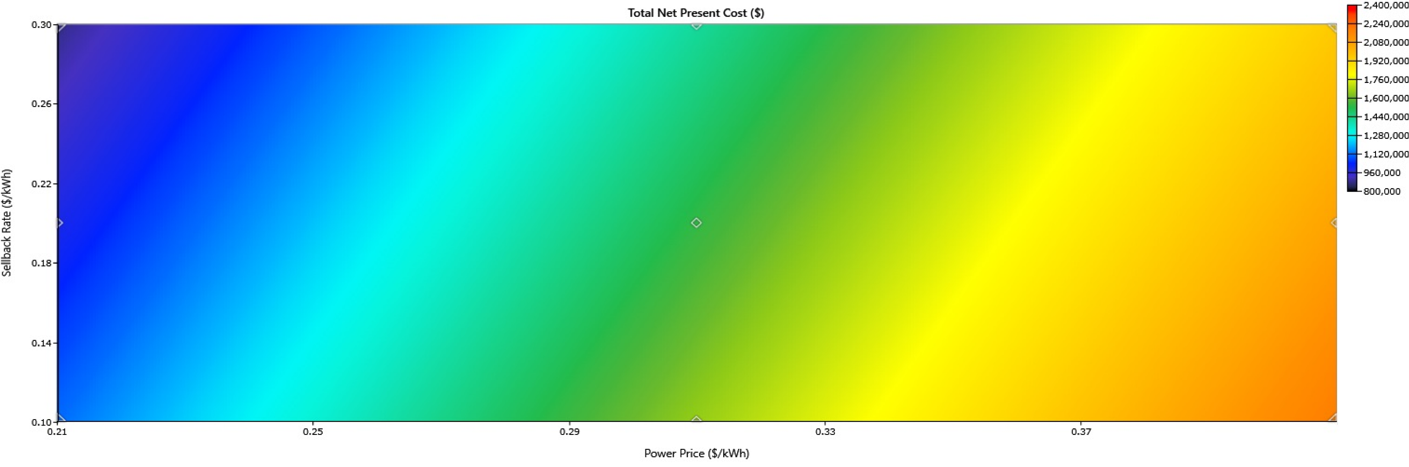
The operational cost significantly depends on the grid purchase price and sell-back power purchase. As shown in Figure 10, the different prices of grid purchase and sell-back power can impact the overall performance of the operational cost of the systems. The sensitivity analysis was performed to assess the operation cost of the overall renewable-energy-based system while changing the power generation prices and power sell-back price. The sensitivity analysis in Figure 10 shows that as the sell-back prices increase, the capital cost of the system reduces, where the lowest capital cost is USD 40,000 with the highest selling power to the grid of 0.30. However, the power purchased at this stage is very low, which is practically not possible; the optimal point is USD 80,000, where the grid sell cost is 0.21 USD/kWh and the power purchase is 0.31 USD/kWh. The sensitivity analysis shows that if the cost of the power purchase is set between 0.30 and 0.31, the optimum operational cost can be achieved, whereas increasing the power purchase cost may impact overall operational cost, increasing up to USD 140,000 when purchased at 0.37 USD/kWh and sold back at 0.10 USD/kWh. This sensitivity analysis shows that reducing the cost optimally while installing solar power can significantly reduce the overall operational cost of the system.

Figure 10. Sensitivity analysis for the operational cost under the influence of power-purchase and sell-back scenarios.

5. Conclusions

The research work conducted in this study quantifies the impact of power balance when integrated with solar power for high inductive loads. In the second part of the research, an economic analysis was performed to assess the economic impact of integrating 100 kW of solar power. This study considered large metropolitan pumping stations. We assessed several power–quality trade-offs and found interesting results. The results showed that, while keeping the power factor at unity in inverter-interfaced systems, active power is reduced by 70%. However, the power factor drops sharply because the grid supplies most of the reactive power (59 kVAR), while the solar power provides the active power. Adjusting the reactive power may improve the power factor and balance active and reactive power values. It was found that setting the reactive power of the inverter interface system from unity to 0.9 reduced reactive power supply from the grid by 66%. It improved the power factor from 0.50 to 0.9 in the unity power factor case. On the other hand, when reactive power compensation is balanced with active power, integrating solar power into the system can provide encouraging economic benefits, with a payback period of approximately 2 years. In the future, the controlling mechanisms for reactive power compensation at load side may even provide better results when integrated with battery energy storage systems (BESSs) with solar power integration.

References

- Reis, A.L.; Lopes, M.A.; Andrade-Campos, A.; Antunes, C.H. A review of operational control strategies in water supply systems for energy and cost efficiency. Renew. Sustain. Energy Rev. 2023, 175, 113140. [Google Scholar] [CrossRef] [Scilit]
- Bititci, N.S.S.; Kumar, U.S.; Chan, V. State of the art literature review on performance measurement. Comput. Ind. Eng. 2011, 60, 279–290. [Google Scholar] [CrossRef] [Scilit]
- Zaman, D.; Tiwari, M.K.; Gupta, A.K.; Sen, D. Performance indicators-based energy sustainability in urban water distribution networks: A state-of-art review and conceptual framework. Sustain. Cities Soc. 2021, 72, 103036. [Google Scholar] [CrossRef] [Scilit]
- Japan International Cooperation Agency. Preparatory Survey Report on the Project for Energy Saving in Water Supply System in Lahore; Japan International Cooperation Agency: Tokyo, Japan, 2014.
- Miao, Q.; Wang, J.; Chao, L. Energy-Saving Optimization of Water Supply Pumping Station Life Cycle Based on BIM Technology. In IOP Conf. Series: Earth and Environmental Science; IOP Publishing: Bristol, UK, 2017; Volume 100, p. 012201. [Google Scholar]
- Gómez, E.; del Teso, R.; Cabrera, E.; Cabrera, E.; Soriano, J. Labeling Water Transport Efficiencies. Water 2018, 10, 935. [Google Scholar] [CrossRef] [Scilit]
- Khadim, M.A.; Al-Zahrani, M.A. Energy-Efficiency Optimization of Water Distribution Networks Using Genetic Algorithms. J. Water Supply Res. Technol.-Aqua 2019, 68, 543–556. [Google Scholar]
- Bonthuys, G.J.; van Dijk, M.; Cavazzini, G. Leveraging Water Infrastructure Asset Management for Energy Recovery and Leakage Reduction. Sustain. Cities Soc. 2019, 46, 101434. [Google Scholar] [CrossRef] [Scilit]
- Luna, T.; Ribau, J.; Figueiredo, D.; Alves, R. Improving energy efficiency in water supply systems with pump scheduling optimization. J. Clean. Prod. 2019, 213, 342–356. [Google Scholar] [CrossRef] [Scilit]
- Rudra Narsimha Rao, G.; Sharma, K.V. Energy conservation opportunities in municipal water supply systems: A case study. Resour. Energy Dev. 2012, 9, 35–48. [Google Scholar] [CrossRef] [Scilit]
- Papagiannis, F.; Gazzola, P.; Burak, O.; Pokutsa, I. Overhauls in water supply systems in Ukraine: A hydro-economic model of socially responsible planning and cost management. J. Clean. Prod. 2018, 183, 358–369. [Google Scholar] [CrossRef] [Scilit]
- Martin-Candilejo, A.; Santillán, D.; Iglesias, A.; Garrote, L. Optimization of the Design of Water Distribution Systems for Variable Pumping Flow Rates. Water 2020, 12, 359. [Google Scholar] [CrossRef] [Scilit]
- Rohilla, S.K.; Kumar, P.; Matto, M.; Sharda, C. Mainstreaming Energy Efficiency in Urban Water and Wastewater Management in the Wake of Climate Change; Centre for Science and Environment: New Delhi, India, 2017. [Google Scholar]
- Jensen, O.; Nair, S. Integrated Urban Water Management and Water Security: A Comparison of Singapore and Hong Kong. Water 2019, 11, 785. [Google Scholar] [CrossRef] [Scilit]
- Mahmood, F.; Ali, H. Energy-Cost Optimization in Water-Supply System. Pak. Dev. Rev. 2013, 52, 437–446. [Google Scholar] [CrossRef] [Scilit]
- Liu, F.; Tait, S.; Schellart, A.; Mayfield, M.; Boxall, J. Reducing carbon emissions by integrating urban water systems and renewable energy sources at a community scale. Renew. Sustain. Energy Rev. 2020, 123, 109767. [Google Scholar] [CrossRef] [Scilit]
- Sun, C.; Puig, V.; Cembrano, G. Real-Time Control of Urban Water Cycle under Cyber-Physical Systems Framework. Water 2020, 12, 406. [Google Scholar] [CrossRef] [Scilit]
- Azeem, F.; Narejo, G.B.; Shah, U.A. Integration of renewable distributed generation with storage and demand side load management in rural islanded microgrid. Energy Effic. 2020, 13, 217–235. [Google Scholar] [CrossRef] [Scilit]
- Al-Shetwi, A.Q.; Hannan, M.A.; Jern, K.P.; Mansur, M.; Mahlia, T.M.I. Grid-connected renewable energy sources: Review of the recent integration requirements and control methods. J. Clean. Prod. 2020, 253, 119831. [Google Scholar] [CrossRef] [Scilit]
- Shafiullah, M.; Ahmed, S.D.; Al-Sulaiman, F.A. Grid integration challenges and solution strategies for solar PV systems: A review. IEEE Access 2022, 10, 52233–52257. [Google Scholar] [CrossRef] [Scilit]
- Ghani, A.A.; Ramachandaramurthy, V.K.; Yong, J.Y. Design of a master power factor controller for an industrial plant with solar photovoltaic and electric vehicle chargers. Electr. Eng. 2022, 104, 13–25. [Google Scholar] [CrossRef] [Scilit]
- Maharjan, S.; Kumar, D.S.; Khambadkone, A.M. Enhancing the voltage stability of distribution network during PV ramping conditions with variable speed drive loads. Appl. Energy 2020, 264, 114733. [Google Scholar] [CrossRef] [Scilit]
- Dugan, R.C.; McGranaghan, M.F.; Santoso, S.; Beaty, H.W. Electrical Power Systems Quality, 3rd ed.; McGraw-Hill: New York, NY, USA, 2012; Available online: https://books.google.co.zm/books?id=h1iBVtbSeI0C (accessed on day month year).
- IEEE Std 519-2014; IEEE Recommended Practice and Requirements for Harmonic Control in Electric Power Systems. IEEE: New York, NY, USA, 2014.
- Chapman, S.J. Electric Machinery Fundamentals; McGraw-Hill: New York, NY, USA, 2012; Available online: https://books.google.com.pk/books?id=wyHAuQAACAAJ (accessed on day month year).
- Azeem, F.; Memon, Z.A.; Baig, S.; Awan, A.B. A two-way pre-installation assessment framework for microgrids under power systems expansion planning. Sustain. Energy Technol. Assess. 2023, 55, 102920. [Google Scholar] [CrossRef] [Scilit]
Disclaimer/Publisher’s Note: The statements, opinions and data contained in all publications are solely those of the individual author(s) and contributor(s) and not of MDPI and/or the editor(s). MDPI and/or the editor(s) disclaim responsibility for any injury to people or property resulting from any ideas, methods, instructions or products referred to in the content. |
© 2026 by the authors. Licensee MDPI, Basel, Switzerland. This article is an open access article distributed under the terms and conditions of the Creative Commons Attribution (CC BY) license.