Research on Multi-Time-Scale Optimal Scheduling of Hydro–Solar Complementation in the Shuoqu River Basin

Abstract

The integration of high shares of renewable energy into the power grid poses significant challenges to the stable operation of power systems. Hydropower, owing to its rapid response capability and reservoir regulation capacity, can effectively mitigate the volatility and randomness associated with photovoltaic power output. This study adopts the “hydro-regulated photovoltaic generation” approach as its core methodology. First, a six-dimensional complementary comprehensive evaluation indicator system is established, and the weights of each indicator are determined using the Analytic Hierarchy Process. Second, tailored to long-term and short-to-medium-term forecasting requirements, the quantile mapping method and the ARIMA–Prophet model are employed to forecast solar and hydroelectric resource. Finally, based on the Guwa Hydropower Station, a long-term–medium-term–short-term multi-objective optimal dispatch framework is developed. The NSGA-II algorithm is utilized to perform multi-objective optimization targeting power generation and resource utilization efficiency. The results demonstrate that, after long-term optimization, power generation increased by 6.34% compared to the non-optimized scenario; medium-term optimization achieved monthly power generation efficiency improvements of 11.45% during the high-water period; and after short-term optimization, the daily output power fluctuated cyclically between 45 and 129 MW, while the overall output remained smooth.

1. Introduction

The installed capacity of new energy sources—particularly wind power and photovoltaic (PV) systems—has expanded rapidly; as a result, the power system is accelerating its transition into a new-type power system characterized by a high proportion of renewable energy and high penetration of power electronic devices. This evolution has led to a decrease in system inertia and short-circuit capacity, significantly increasing the challenges associated with ensuring safe and stable operation [1]. PV power output is inherently characterized by volatility, randomness, and intermittency; its large-scale integration into the grid thereby intensifies the peak-shaving burden on the power system. In contrast, hydroelectric power plants, leveraging their reservoir capacity for regulation, can effectively smooth out fluctuations in PV power output, representing an important technical approach for addressing both the integration of renewable energy and the maintenance of grid stability [2].

In the context of water–photovoltaic complementary energy system evaluation, Zhao et al. [3] developed a flexibility assessment framework for watershed-based wind–solar–hydropower multi-energy complementary bases that takes into account the complementary characteristics of cascade hydropower stations, thereby providing a quantitative basis for evaluating the capacity matching between water and photovoltaic resources. Zhang et al. [4], from the perspective of capacity allocation, comprehensively considered both power delivery demands and reservoir characteristics to investigate the optimal PV integration capacity for large-scale water–photovoltaic complementary systems, thus offering a quantitative basis for determining the matching relationship between water and photovoltaic resources. Zhang et al. [5] proposed a simulation model that fully integrates long-term water allocation with short-term peak-shaving demands, designed to accurately determine the optimal integration capacity of PV power plants within water–photovoltaic complementary systems.

In the field of complementary scheduling optimization, Wenlin et al. [6] developed a long-term scheduling model for hydro–photovoltaic complementary systems; by introducing a scheduling auxiliary function, they integrated long-term generation objectives and short-term operational performance indicators into the long-term optimal scheduling process, thereby overcoming the limitations imposed by the time-step size in long-term scheduling. Huang et al. [7], addressing issues such as output shortages, wind/photovoltaic curtailment, and hydro curtailment risks in the operation of wind–solar–hydro complementary systems, constructed a complementary scheduling optimization model that balances economic efficiency with operational risks, providing a systematic methodology for economic operation decision-making in such systems. Guo et al. [8], focusing on day-ahead scale complementary scheduling problems, proposed a risk-averse optimization scheduling method that leverages the rapid regulation capability of hydropower to mitigate the stochastic fluctuations in wind and solar power output while satisfying the grid’s demand for stable power supply; Lu et al. [9], tackling the multiple uncertainties associated with runoff and photovoltaic output in long-term scheduling for cascade hydro–photovoltaic complementary systems, proposed a medium-to-long-term scheduling method based on interval optimization; by defining appropriate uncertainty intervals for the decision variables, this method enhances the adaptability and robustness of the scheduling scheme in actual operation; Su et al. [10] developed a real-time rolling optimization scheduling framework based on model predictive control; through a cyclic mechanism comprising rolling prediction–rolling optimization–rolling execution, this framework enables rapid response to and dynamic adjustment of photovoltaic output fluctuations. Zhu et al. [11] developed a coordinated optimization framework for the long-term joint operation of large-scale hydropower–photovoltaic complementary systems and designed a parallel GFM-MOEA algorithm to search for Pareto-optimal solutions; by integrating the SMAA-FOS robust decision-making model, they enhanced the reliability of the scheduling schemes under uncertain conditions. Xu et al. [12], while accounting for electricity price factors, derived long-term operational rules for hybrid hydropower–wind–photovoltaic energy systems, revealing the driving influence of electricity price fluctuations on hydropower dispatching decisions.

However, current research predominantly focuses on the computational efficiency and integration effectiveness at a single time scale (e.g., day-ahead or intra-day), while there is insufficient depth of investigation into multi-time-scale coordination. To address this gap, some scholars have begun exploring coordinated scheduling across multiple time scales. Shen et al. [13] proposed a multi-time-scale scheduling optimization method for cascade hydro–photovoltaic complementary systems that accounts for spatiotemporal correlations; by employing Frank-copula correlation analysis to identify the spatiotemporal interaction characteristics of hydro and photovoltaic resources, they demonstrated the feasibility of multi-time-scale-coordinated scheduling in enhancing photovoltaic power integration capabilities. However, this article further integrates complementary resource assessment, temporal scale prediction, and reservoir boundary transfer within a unified research framework. Cheng et al. [14], addressing the high computational complexity associated with modeling the coupling between medium-to-long-term and short-term operational decisions, introduced deep learning models as an alternative to traditional explicit coupling approaches; these models are used to capture the intrinsic relationships among short-term, medium-term, and long-term operational decisions, thereby bringing the system’s optimization outcomes closer to the theoretically optimal solution. This article employs a top-down boundary transmission mechanism with well-defined physical meanings: long-term scheduling establishes the water volume and operational boundaries; medium-term planning further decomposes these boundaries and transmits them to the short-term horizon; and in the short term, hydropower regulation capacity is utilized within these pre-defined boundaries to compensate for fluctuations in photovoltaic generation. Liu et al. [15] proposed a multi-stage nested coordinated optimization scheduling model for hydro, wind, and solar power systems based on opportunistic constraints to mitigate wind and solar power curtailment issues arising from insufficient transmission line capacity. The study by Cheng et al. is the closest to this article. Cheng et al. [16], tackling the problem of the fragmented medium- and short-term scheduling processes and the lack of a unified coupling framework in hydro–wind–solar complementary systems, developed a medium-and long-term complementary scheduling coupled with a short-term power balance model; this model was applied to large-scale renewable energy bases, revealing the collaborative and competitive mechanisms under various multi-energy interaction scenarios.

In conclusion, existing studies on hydro–photovoltaic complementary systems have increasingly recognized the role of hydropower flexibility in mitigating photovoltaic fluctuations, but the integrated coordination of hydropower regulation across multiple scheduling horizons remains insufficiently explored. This study therefore develops an integrated multi-time-scale dispatch framework centered on hydropower regulation of photovoltaic output. By linking resource complementarity assessment, multi-scale resource forecasting, and hierarchical optimization, the proposed framework coordinates long-term water-resource allocation, medium-term water-use scheduling, and short-term photovoltaic fluctuation compensation.

Specifically, the contributions of this paper can be divided into the following three parts: (1) A six-dimensional hydro–solar complementarity assessment is established to characterize resource complementarity from correlation, seasonal, fluctuation, regulation, capacity matching, and cascade synergy dimensions, providing a resource-level basis for subsequent scheduling. (2) A time-scale-matched forecasting framework is developed, in which quantile mapping forecasting is used for long-term resource characterization, while an ARIMA–Prophet fusion model with error-based reciprocal weighting is used for medium- and short-term resource prediction. The predictive data primarily serve as data inputs for assessing the complementarity of hydroelectric and solar power resources. (3) Medium-, long-, and short-term dispatch calculations are performed via retrospective optimization based on historical observation data. A hierarchical long-to-medium-to-short-term scheduling framework is constructed in which reservoir-state and generation boundaries are progressively transferred from longer to shorter horizons. Within these boundaries, hydropower is actively used to regulate photovoltaic output at the short-term scale. The present implementation adopts explicit top-down boundary transfer, thereby maintaining physical interpretability and computational decomposition.

2. Methodology

The Shuoqu River is part of the Jinsha River water system. According to relevant water security planning data from Xiangcheng County, the total drainage area of the Shuoqu River is approximately 10,987.1 km², of which the area within Xiangcheng County accounts for approximately 2192.5 km²; the length of the river within the county is about 122.1 km, the average gradient of the river channel is approximately 12‰, the total elevation drop is about 1427.35 m, the multi-year average discharge is approximately 66.3 m³/s, and the multi-year average annual runoff is approximately 2.091 billion m³. These figures indicate that the study area possesses a large drainage basin scale and pronounced topographic relief. Regarding the specific locations of the water–solar complementary projects, the Guwa Hydropower Station is situated in the upper reaches of the Shuoqu River, with the project area at an elevation of approximately 3000 m; in contrast, the supporting Lela Photovoltaic Power Station is located at an elevation of approximately 4600 m, approximately 18 km from the Guwa Hydropower Station, creating a significant elevation difference of about 1600 m.

This study takes the Guwa–Lela Hydropower–Photovoltaic System in the Shuoku River Basin as its research subject and establishes a research framework encompassing “resource assessment–resource forecasting–multi-time-scale optimization”. First, a complementary comprehensive evaluation indicator system is developed to quantify the complementary potential of hydro–photovoltaic resources; second, tailored to the forecasting requirements at both long-term and medium-to-short-term time scales, the quantile mapping method [17] and an ARIMA–Prophet fusion model are employed to obtain high-precision hydro–photovoltaic resource forecasting data; finally, a long-term–medium-term–short-term multi-objective optimization framework is constructed and solved using the NSGA-II algorithm to achieve the synergistic optimization of power generation benefits and resource utilization efficiency.

2.1. Water–Solar Energy Complementarity Comprehensive Evaluation Indicator System

To quantitatively assess the complementary potential of water and solar resources within a watershed, this study establishes a six-dimensional complementarity evaluation system that encompasses the Correlation Index, Seasonal Complementarity Index, Fluctuation Complementarity Index, Regulation Index, Capacity Matching Index, and Cascade Synergy Index.

(1) Correlation Index

The Pearson correlation coefficient is used to measure the linear correlation r between solar irradiance and runoff, and the correlation coefficient is then linearly mapped onto the [0, 1] interval:

$$r={\displaystyle \frac{{\displaystyle \sum _{t=1}^T(G(t)-\overline{G})(Q(t)-\overline{Q})}}{\sqrt{{\displaystyle \sum _{t=1}^T{(G(t)-\overline{G})}^2{\displaystyle \sum _{t=1}^T{(Q(t)-\overline{Q})}^2}}}}}$$

(1)

$$I_{\mathrm{corr}}={\displaystyle \frac{1-r}{2}}$$

(2)

G(t) denotes solar irradiance (W/m²), Q(t) denotes river runoff rate (m³/s), and r denotes the Pearson correlation coefficient between photovoltaic and hydroelectric power output sequences. r ∈ [−1,1]. When r = −1 (perfect negative correlation), and I_corr = 1, it indicates optimal complementarity; when r = 1 (perfect positive correlation), and I_corr = 0, it indicates poorest complementarity; and when r = 0, and I_corr = 0.5, it represents a reference point for moderate complementarity. This index converts the statistical correlation coefficient into a standardized complementarity measure that can be directly incorporated into weighted calculations.

(2) Seasonal Complementarity Index

This approach uses the I_season stability of the seasonal correlation coefficients to reflect the persistence of complementary relationships over the seasonal scale; its construction methodology is consistent with that of the Correlation Index, and it essentially represents a decomposition and reweighting of the Correlation Index across the seasonal dimension.

$$I_{\mathrm{season}}={\displaystyle \frac{1}{4}}{\displaystyle \sum _{s=1}^4\frac{1-r_s}{2}}$$

(3)

r_s denotes the correlation coefficient for each season, reflecting the stability of seasonal complementarity.

(3) Volatility Complementarity Index

The Fluctuation I_fluct Complementarity Index measures the proportion of time periods in which the daily power output variations in photovoltaic and hydroelectric systems move in opposite directions relative to the total time period, reflecting the complementary capability at the short-term fluctuation level.

$$\left\{\begin{array}{l}{I}_{\mathrm{fluent}}={\displaystyle \frac{1}{T-1}}{\displaystyle \sum _{t=1}^{T-1}\left[\Delta G\left(t\right)\cdot \Delta Q\left(t\right)\right]}\\ \Delta G\left(t\right)=G\left(t\right)-G\left(t-1\right)\\ \Delta Q\left(t\right)=Q\left(t\right)-Q\left(t-1\right)\end{array}\right.$$

(4)

(4) Adjustment Capability Index

The cascade total regulation coefficient is defined as the ratio of the total storage capacity to the annual average runoff:

$$I_{\mathrm{reg}}={\displaystyle \frac{V_{\mathrm{total}}}{W_{\mathrm{annual}}}}$$

(5)

V_total denotes the total storage capacity of the reservoir (m³), and W_annual denotes the total annual runoff volume (m³). A larger value indicates a stronger interannual and seasonal regulation capacity of the reservoir for runoff, thereby providing an adequate compensation margin to accommodate fluctuations in photovoltaic power generation.

(5) Capacity Matching Index

Based on the assessment of the compatibility between photovoltaic and hydroelectric power systems, the normalized evaluation range for the Capacity Matching Index in this study is set between 0.5 and 1.5; if this range is exceeded, the complementary effect will exhibit a slight decline.

$$I_{\mathrm{cap}}=\left\{\begin{array}{cc}{\displaystyle \frac{C_{\mathrm{PV}}/C_{\mathrm{H}}}{0.5}},& C_{\mathrm{PV}}/C_{\mathrm{H}}<0.5\\ 1,& 0.5\le C_{\mathrm{PV}}/C_{\mathrm{H}}\le 1.5\\ \max \left(0,1-{\displaystyle \frac{C_{\mathrm{PV}}/C_{\mathrm{H}}-1.5}{2}}\right),& C_{\mathrm{PV}}/C_{\mathrm{H}}>1.5\end{array}\right.$$

(6)

C_PV denotes the rated capacity of the photovoltaic power station (MW), and C_H denotes the rated installed capacity of the hydroelectric power station (MW).

(6) Cascade Synergy Index

The cascade synergy I_syn index increases as the number of cascade stages (n) increases, reflecting the additional benefit in complementary capacity associated with the joint regulation of multiple reservoirs compared to the operation of a single reservoir.

$$I_{\mathrm{syn}}=\min \left(1, {\displaystyle \frac{n}{10}}+0.2\right)$$

(7)

2.2. Multi-Time-Scale Prediction Method for Water and Energy Resources

2.2.1. Long-Term Forecasting: Quantile Mapping Method

Within the study area, even if two energy facilities are relatively close in horizontal distance, their solar radiation, temperature, and precipitation conditions may differ significantly due to variations in elevation, slope aspect, and topographic shading. Consequently, employing a single spatial scale to directly characterize the solar energy resources across the entire study area may obscure local spatial heterogeneities.

Based on their study using a topographic radiation model over the Tibetan Plateau, Xian et al. [18] found that the influence of topography on surface shortwave radiation intensifies with increasing slope gradient; in steep areas where the slope exceeds 15°, the topographic radiation forcing can reach 9.5% of the annual mean shortwave radiation. More importantly, even when the spatial resolution is reduced to 5 km, the topographic effect remains pronounced, exhibiting significant seasonal and slope aspect-dependent variations. Compared to the low resolution of the original climate model, the 2 km × 2 km resolution better captures large-scale topographic and resource spatial gradients within the study region.

The quantile mapping method corrects the statistical distribution of the model’s output to match the distribution characteristics of the observed data by establishing a mapping relationship between the simulated and observed data on their cumulative distribution functions (CDFs), thereby eliminating systematic bias. Let F_m,hist(x) denote the cumulative distribution function of the model’s simulated data over the historical period, and let F_obs(x) denote the cumulative distribution function of the observed data over the same period. For any raw output value x_m generated by the model for a future period, the quantile mapping method applies correction based on the “equal-probability transformation” principle [19]:

$$F_{\mathrm{obs}}\left(\stackrel{\wedge }{{\displaystyle x}}\right)=F_{m,\mathrm{hist}}\left(x_m\right)$$

(8)

The quantile position of the original model data within its own distribution corresponds to the quantile position of the corrected data within the observed distribution. However, the validity of this method depends on the “bias stationarity assumption”—namely, that the statistical characteristics of the model’s systematic bias do not change over time.

2.2.2. Short-to-Medium-Term Forecasting: ARIMA–Prophet Fusion Model

The solar radiation observation series exhibits characteristics such as strong annual cyclical seasonality, non-stationary trend variations, and multi-scale random disturbances; therefore, a single linear model is insufficient to simultaneously capture both its trend and cyclical structures. To address this, we develop a hybrid ARIMA–Prophet forecasting model: the ARIMA [20] component is used to extract the linear trend and short-term autocorrelation features of the series; the model is specified as ARIMA(p,d,q), where the order of differencing (d) is determined via an ADF stationarity test, and the optimal order is identified through grid search within a specified range p,q ∈ [0,3] based on the BIC criterion; the Prophet [21] component decomposes the time series into an additive structure consisting of a trend term, a cyclical term, a holiday term, and an error term:

$$y\left(t\right)=g\left(t\right)+s\left(t\right)+h\left(t\right)+{\epsilon }_t$$

(9)

g(t) denotes the trend term, s(t) denotes the cyclical term (annual or weekly cycle), h(t) denotes for the holiday effect term, and u is the error term. This study extracts the annual cyclical component and constructs a phase-position encoding for solar radiation over the annual cycle.

The predicted values from the two models are weighted and fused using the reciprocal of the root mean square error (RMSE) based on the 1095-day historical forecast [20,21]:

$${\widehat{y}}_{\mathrm{fusion}}(t)=w_{\mathrm{ARIMA}}(t)\cdot {\widehat{y}}_{\mathrm{ARIMA}}(t)+w_{\mathrm{Prophet}}(t)\cdot {\widehat{y}}_{\mathrm{Prophet}}(t)$$

(10)

$$\left\{\begin{array}{l}\begin{array}{c}{w}_{\mathrm{ARIMA}}(t)={\displaystyle \frac{{\mathrm{RMSE}}_{\mathrm{Prophet}}(t)}{{\mathrm{RMSE}}_{\mathrm{ARIMA}}(t)+{\mathrm{RMSE}}_{\mathrm{Prophet}}(t)}}\\ w_{\mathrm{Prophet}}(t)={\displaystyle \frac{{\mathrm{RMSE}}_{\mathrm{ARIMA}}(t)}{{\mathrm{RMSE}}_{\mathrm{ARIMA}}(t)+{\mathrm{RMSE}}_{\mathrm{Prophet}}(t)}}\end{array}\\ \mathrm{RMSE}\left(t\right)=\sqrt{{\displaystyle \frac{1}{L}}{\displaystyle \sum _{\tau =t-L}^{t-1}{e}^2(\tau )}}\end{array}\right.$$

(11)

e(τ) denotes the sequence of model prediction errors over the 1095-day preceding time point, and $\widehat{\mathrm{y}}\left(\mathrm{t}\right)$ denotes the predicted value from the forecasting model at time point.

2.3. Single-Stage Multi-Time-Scale Multi-Objective Optimization Scheduling Model

Grid-connected power balance relationship: the hydro–photovoltaic complementary system leverages the fast response capability and energy storage characteristics of hydroelectric power to compensate for the stochastic nature and reverse peak-shaving behavior of photovoltaic output; the system’s grid-connected power P(t) is expressed as follows:

$$P\left(t\right)=P_{\mathrm{PV}}\left(t\right)+{\displaystyle \sum _{i=1}^N{P}_{\mathrm{hy},i}}\left(t\right)$$

(12)

P_PV(t) denotes the actual photovoltaic power output (W); P_hy,t(t) denotes the power output of the i-th hydropower station (W); and N is the number of cascade stages (for single-stage power stations, N = 1). This equation serves as the fundamental power balance constraint in the multi-objective optimization model.

In dispatch optimization, the calculation of hydropower generation output consistently employs physical relationships based on discharge rate, net head, and generator output coefficients. In long-, medium-, and short-term scheduling programs, the downstream water level is first determined from the discharge rate and the downstream flow rate using the DQH curve; subsequently, the net operating head and the output power of the hydropower station are calculated by subtracting the downstream water level from the average upstream water levels at the beginning and end of the time interval (m), and then accounting for the head loss associated with the discharge rate.

$$H_t=Z_t^{\mathrm{up}}-Z_t^{\mathrm{down}}-h_t^{\mathrm{loss}}$$

(13)

$$P_{\mathrm{H},t}={\eta }_i\cdot \rho \cdot g\cdot Q_t\cdot H_t$$

(14)

P_H,t denotes the output power of the hydroelectric power station during the time interval t (W); Q_t denotes the power generation flow rate of the hydroelectric power station during the time interval t (m³/s); and H_t denotes the net power generation head of the hydroelectric power station during the time interval t (m).

The three-tiered nested framework—comprising long-term, medium-term, and short-term scales—divides optimal decision-making into these three temporal dimensions based on the monsoon climate characteristics of continental plateaus within river basins and the multi-scale fluctuation patterns of photovoltaic and runoff resources. The long-term scale (annual cycle, monthly time step; T = 12, Δt = 720 h) focuses on the annual interannual allocation of water resources and the overall distribution of electricity generation; the medium-term scale (monthly cycle, daily time step; T equals the number of days in the current month, Δt = 24 h) bridges long-term and short-term objectives by employing monthly weather forecasts to perform fine-grained allocation of daily water usage; and the short-term scale (daily cycle, 15 min time step; T = 96) is responsible for real-time compensation of fluctuations in photovoltaic power output. These three scales are hierarchically nested and coupled through water level boundaries and power generation constraints; the medium-and long-term scales determine the initial and final water levels for each time interval as well as the total electricity generation; the short-term scale then performs fine-grained adjustments within this framework, although insufficient regulation reservoir capacity at the medium-and long-term stages will directly constrain the short-term load tracking capability.

The long-and medium-term optimization objectives are to minimize water curtailment, maximize total benefit, and maximize adjustability.

$$f_{1,l}=\min {\displaystyle \sum _t^T{Q}_{\mathrm{spill},t}\cdot \Delta t}$$

(15)

Q_spill,t denotes the curtailed water flow of the hydropower station during the time interval (m³/s).

$$f_{2,l}=\max {\displaystyle \sum _{t=1}^T\left[c_{\mathrm{H}}{P}_{\mathrm{H},t}\Delta t+c_{\mathrm{PV}}{P}_{\mathrm{PV},\mathrm{used},t}\Delta t-c_{\mathrm{curt}}{P}_{\mathrm{PV},\mathrm{curt},t}\Delta t\right]}$$

(16)

c_H denotes hydropower feed-in tariff (yuan/(kW·h)), c_PV denotes photovoltaic feed-in tariff (yuan/(kW·h)), c_curt denotes reneged photovoltaic penalty tariff (yuan/(kW·h)), P_PV,used,t denotes actual photovoltaic power utilized (W), and P_PV,curt,t denotes discarded optical power (W).

$$f_{3,l}=\max {\displaystyle \sum _{t=1}^T\left[P_{\mathrm{H},t}^{\max }\left(Z_t\right)-P_{\mathrm{H},t}^{\min }\left(Z_t\right)\right]}$$

(17)

$P_{\mathrm{H},t}^{\max }\left(Z_t\right)$ denotes maximum power output of the hydroelectric power station (W), $P_{\mathrm{H},t}^{\min }\left(Z_t\right)$ denotes lower limit of hydropower plant output (W).

The short-term optimization objectives are to minimize load tracking deviation, maximize short-term adjustability, and minimize output variability.

$$f_1^s=\min {\displaystyle \sum _{t=1}^T{\left(P_{\mathrm{load}}(t)-\left(P_{\mathrm{PV}}(t)+P_{\mathrm{H}}\left(t\right)\right)\right)}^2}$$

(18)

This formula ensures that the system exhibits favorable tracking performance, with the objective of minimizing the deviation between the system’s operating point output and the load setpoint.

$$f_2^s=\max {\displaystyle \sum _{t=1}^T\min \left(P_{\mathrm{H},t}^{\max }(t)-P_{\mathrm{H},t}(t),P_{\mathrm{H},t}(t)-P_{\mathrm{H},t}^{\min }(t)\right)}$$

(19)

In short-term operation, adjustability is manifested as residual adjustable capacity, which is utilized to mitigate ultra-short-term forecasting errors in photovoltaic systems; this formulation ensures that the system maintains sufficient upper and lower adjustment margins at all times.

$$f_3^s=\min {\displaystyle \sum _{t=1}^{T-1}{\left(P_{\mathrm{H},t}(t+1)-P_{\mathrm{H},t}(t)\right)}^2}$$

(20)

In the short-term dispatch phase, the smoothness of hydropower output profiles is used to assess system operational stability.

The model is subject to various physical constraints—including water balance, reservoir water level, upper and lower limits on power station output, discharge rate, daily water level variation range, output ramp rate, and avoidance of unit vibration zones—thereby forming a high-dimensional, nonlinear, and strongly coupled multi-objective optimization problem.

$$\begin{array}{cc}{V}_{t+1}=V_t+(Q_{\mathrm{in},t}-Q_t-S_t-O_t)\Delta t& \forall t\in T\end{array}$$

(21)

V_t+1 denotes initial reservoir water storage of the power plant during the t + 1-th time interval (m³), Q_in,t denotes inlet flow rate to the power station during time interval t (m³/s), S_t denotes discharge flow rate of the power station during time interval t (m³/s), and O_t denotes other water usage in the t-th time interval of the power station (m³/s).

$$\begin{array}{cc}{\underset{\_}{Z}}_t\le Z_t\le {\overline{Z}}_t& \forall t\in T\end{array}$$

(22)

${\underset{\_}{Z}}_t$ denotes the lower water level limit at the beginning of the T time period of the power station (m), ${\overline{Z}}_t$ denotes the upper water level limit of the power station during the T time period (m), and $Z_t$ denotes the reservoir water level at the beginning of time interval t at the power station (m), which is identical to the upstream reservoir water level.

$$\begin{array}{cc}{N}_{\min }\le A\times Q_t\times H_t\le N_{\max }& \forall t\in T\end{array}$$

(23)

N_min denotes allowable minimum output of the power plant (W), and N_max denotes the installed capacity of the power plant (W).

$$\begin{array}{cc}{Q}_t^{\min }\le Q_{\mathrm{out},t}\le Q_t^{\max }& \forall t\in T\end{array}$$

(24)

$Q_t^{\min }$ denotes the minimum discharge rate to be ensured by the power station during time interval t (m³/s), and $Q_t^{\max }$ denotes maximum allowable discharge flow rate of the power station during time interval t (m³/s).

$$\left|Z(t+1)-Z(t)\right|\le \Delta Z_{\max }$$

(25)

$\Delta Z_{\max }$ denotes permitted daily water level variation for the reservoir (m).

$$\left|P_H(t+1)-P_{\mathrm{H}}(t)\right|\le R_{\max }^{\mathrm{ramp}}\Delta t$$

(26)

$R_{\max }^{\mathrm{ramp}}$ denotes maximum allowable ramp rate of the power plant (W/h).

$$\begin{array}{cc}\left(p_{i,n,t}-p_n^{\mathrm{low}}\right)\left(p_{i,n,t}-p_n^{\mathrm{up}}\right)\ge 0,& \forall i,n,t\end{array}$$

(27)

$p_n^{\mathrm{low}}$ denotes lower limit of the unit vibration zone, and $p_n^{\mathrm{up}}$ denotes upper limit of the unit vibration zone.

The scheduling optimization problem for water–photovoltaic complementary systems is characterized by high dimensionality, nonlinearity, strong coupling, and the presence of multiple conflicting objectives. In this study, the NSGA-II algorithm [22], which is based on genetic algorithms, is selected as the solver—primarily due to its natural suitability for multi-objective Pareto optimization, its strong robustness in handling non-convex and discontinuous feasible regions, and its capability to maintain population diversity.

NSGA-II is employed to obtain a set of non-dominated solutions for the multi-objective scheduling problem presented in this paper, thereby revealing the trade-offs among profit, water diversion, adjustability, and short-term power stability. In the long-term optimization phase, the population size is set to 200, with a crossover probability of 0.90, a mutation probability of 0.10, and a maximum number of evolutionary generations constrained to 100. The crossover operator employs Blend Crossover with parameter α = 0.5, while the mutation operator uses Gaussian Mutation with mean μ = 0, standard deviation σ = 1, and a per-gene mutation probability of 0.10. Environmental selection is performed using the NSGA-II non-dominance sorting operator. For the medium-term optimization phase, NSGA-II is likewise employed, although its decision variables and objective function formulation differ from those in the long-term phase. The algorithm parameters are set as follows: population size = 200, maximum number of generations = 100, crossover probability = 0.90, and mutation probability = 0.10; crossover employs Blend Crossover (α = 0.5), mutation employs Gaussian Mutation (μ = 0, σ = 1, single-gene mutation probability = 0.2), and environmental selection utilizes the non-dominance sorting mechanism of NSGA-II. In the short-term scheduling phase, the population size is also set to 200, with a crossover probability of 0.90, a mutation probability of 0.10, and a maximum number of evolutionary generations set to 100. The crossover operator again employs Blend Crossover (α = 0.5), the Gaussian Mutation parameters are set to μ = 0 and σ = 5, the per-gene mutation probability remains 0.10, and environmental selection is likewise performed using the NSGA-II non-dominance sorting mechanism.

The long-term optimization employs real-number encoding, using monthly scale water level variations as the primary decision variables. For the Guwa Hydropower Station, each individual comprises 11 consecutive water level decision variables, corresponding to the water levels from early July to early May of the following year; the water levels at the beginning and end of June of each year serve as fixed boundary conditions. During the individual evaluation phase, the decision variables are first subjected to boundary processing; subsequently, the discharge and power generation flows for the respective time periods are calculated based on the water level–reservoir capacity relationship, while constraints such as ecological flow requirements and the maximum allowable power generation flow are verified. In the medium-term optimization phase, daily scale water levels within the current month are adopted as decision variables, with boundary conditions at the beginning and end of each month derived from the long-term optimization results. Boundary corrections are applied during individual evaluation, and constraints pertaining to water level, flow rate, and other operational parameters are checked; if the degree of constraint violation exceeds 10⁻⁶, the individual solution is deemed infeasible. After 100 evolutionary generations, the final Pareto non-dominated solution set is extracted, sorted according to power generation revenue, and the solution achieving the median power generation revenue level is selected as the representative compromise solution. The corresponding boundary conditions are then passed to the short-term optimization phase. The short-term optimization employs daily scale data with a 15 min time resolution, comprising a total of 96 time intervals, with power generation flow rate as the core decision variable. Based on actual photovoltaic power output, fine-grained decision-making is applied to the corresponding time intervals when the PV output exceeds 0.01 MW; for intervals where no effective PV output is available, coarse-grained representation is employed. The discharge is constrained within the range of 0–87.80 m³/s. During the hourly evaluation process, the reservoir water level is updated based on the water balance equation, while operational constraints—including ecological base flow, water level upper and lower limits, and the maximum power output of the hydropower station—are also verified. After completing evaluations for 96 hourly intervals, the final water level is checked, allowing a deviation of ±0.5 m from this value; if this terminal constraint is not satisfied, the individual scenario is deemed infeasible.

Taking short-term complementary scheduling as an example, for the load tracking deviation F₁ and output volatility F₃, we employ a Min–Max normalized form: Z₁(x) = [F₁(x) − F₁min]/[F₁max − F₁min], and Z₃(x) = [F₃(x) − F₃min]/[F₃max − F₃min]. For the short-term adjustable capacity F₂, which is a maximization objective, we convert it to an equivalent minimization form: Z₂(x) = 1 − [F₂(x) − F₂min]/[F₂max − F₂min]. After these transformations, all three indicators are converted into dimensionless quantities following the principle that “the smaller the value, the better.” On this basis, we then apply pre-defined decision preference weights: w₁ = 0.80, w₂ = 0.15, w₃ = 0.05, and compute: J(x) = 0.80Z₁(x) + 0.15Z₂(x) + 0.05Z₃(x). The non-dominated solution yielding the smallest value of J(x) is selected as the representative operating scheme for the short-term scheduling phase.

2.4. Description of the Guwa Hydropower Station

This study takes the Guwa–Lela Hydropower–Photovoltaic System in the Shuoku River Basin as its research subject. The operating parameters of the Guwa Hydropower Station are presented in Table 1.

Table 1. Operating parameters of the Guwa Hydropower Station.

Parameter Name	Numeric Value	Role in the Model
Reservoir storage capacity	2.39 × 108 m3	The capacity bound defining the water balance constraint.
installed capacity	205 MW	Determine the physical reference for the output upper-bound constraint.
Regulating storage capacity	2.23 × 108 m3	Used to calculate the storage coefficient β and determine the regulation capacity level.
Annual runoff volume	1.72 × 109 m3	Denominator term for calculating the storage capacity coefficient.
Output	Max: 205 MW Min: 53 MW	Output constraint determines the feasible solution boundary.
Waterhead	Max: 314.9 m Min: 212.7 m	Value boundary for the nonlinear waterhead–output mapping.
Short-term adjustment coefficient	0.025	Short-term decision variable scoring calculation basis.
Mid-term adjustment coefficient	0.501	Mid-term decision variable scoring basis.
Long-term adjustment coefficient	0.938	Long-term decision variable scoring basis.

Notes: definition of the adjustment coefficient: $R_{\mathrm{reg}}={\displaystyle \frac{V_{\mathrm{total}}}{W_{\mathrm{annual}}}}$.

Where R_reg denotes accommodation coefficient, V_total denotes total reservoir capacity (m³), W_annual denotes annual total runoff (m³). The value “53 MW” in Table 1 denotes the minimum operating output reference value for the hydroelectric power station; this should be interpreted as the operational boundary when the generating unit is in operation, rather than being directly understood as the “average power lower limit” across all time scales.

3. Results and Discussion

The results of the investigation are presented and discussed in this section for the three stages carried out.

3.1. Water–Solar Energy Complementarity Comprehensive Evaluation Results

After normalizing the six sub-indicators, the Analytic Hierarchy Process (AHP) [23] was employed to determine their weights and perform weighted synthesis (Table 2). The AHP method determines the relative importance of each indicator by constructing a judgment matrix, using the Saaty pairwise comparison scale, and performing a consistency check (CR < 0.1); to improve reproducibility, the final weights were determined based on the constructed pairwise comparison matrix and subsequently examined through consistency and weight-sensitivity analyses. Ultimately, the Regulation Capability Index was assigned the highest weight of 0.25, while the Seasonal Complementarity and Fluctuation Complementarity Indexes were each assigned a weight of 0.15; the Capacity Matching Index and the Cascade Synergy Index were established as auxiliary indicators.

Table 2. Complementary composite index weights.

Metric	Relativity Index	Seasonal Complementarity Index	Fluctuation Complementarity Index	Regulation Index	Capacity Matching Index	Cascade Synergy Index
exponential quantity	0.35	0.43	0.479	0.4	0.6	0.7
weighted value	0.20	0.15	0.15	0.25	0.15	0.1

Notes: Equation (7) is employed to represent the cascaded coordination relationships in a general n-stage cascade hydropower system, serving to describe the additional coordinated regulation capability that emerges as the number of cascade stages increases. For the specific case studies presented in this paper, the primary focus has been on conducting single-plant dispatch optimization centered around the Guwa Hydropower Station; consequently, the Isyn corresponding to Equation (7) has not been directly incorporated as either the objective function or a constraint in the NSGA-II algorithm. The research scope of both the original and revised versions of this paper has also been explicitly delineated, and the current study has not yet fully accounted for the coordinated regulation capability among multiple cascade stages. The value 0.70 in Table 2 is an auxiliary normalization quantity in the six-dimensional complementary evaluation table, rather than an Isyn value directly computed from Equation (7) for the current single-stage case study.

Based on the physical significance of the six criteria, the research objectives, and their interrelationships within the hydro–solar complementary system, we constructed a single pairwise comparison matrix using the Saaty pairwise comparison scale, yielding the following judgment matrix:

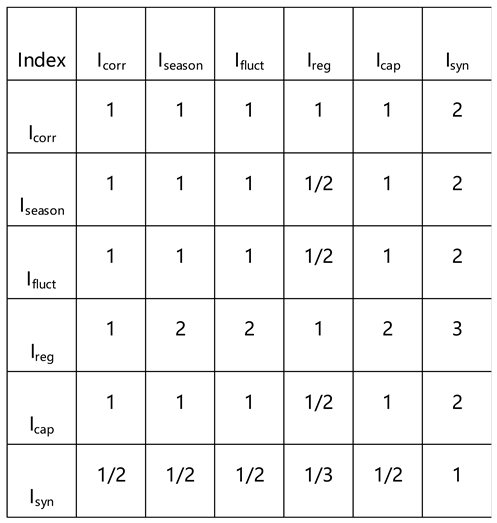
The six rows and six columns correspond, respectively, to the Correlation Index, Seasonal Complementarity Index, Fluctuation Complementarity Index, Regulation Capability Index, Capacity Matching Index, and Cascade Synergy Index.

Using the largest eigenvalue method, the following results were obtained:

$${\lambda }_{\max }=6.0523$$

It further follows that

$$CI={\displaystyle \frac{{\lambda }_{\max }-n}{n-1}}={\displaystyle \frac{6.0523-6}{6-1}}=0.0105$$

Given a sixth-order judgment matrix $RI=1.24$, the random consistency index is calculated as follows:

$$CR={\displaystyle \frac{CI}{RI}}={\displaystyle \frac{0.0105}{1.24}}=0.0084$$

Therefore, the judgment matrix passed the consistency test.

The weights obtained from the judgment matrix are approximately: w = (0.1788, 0.1565, 0.1565, 0.2699, 0.1565, 0.0820). It can be observed that the weight structure derived from the judgment matrix aligns with the benchmark weights ultimately adopted in this study. The values (0.20, 0.15, 0.15, 0.25, 0.15, 0.10) exhibit relatively good consistency, with the Regulation Capability Index consistently ranking highest in importance, while the Cascade Synergy Index primarily serves an auxiliary evaluative role.

We conducted a single-factor weight perturbation analysis using the data from Table 2 in this paper. The six indicator values in Table 2 are 0.35, 0.43, 0.479, 0.40, 0.60, and 0.70, respectively, while the baseline weights are 0.20, 0.15, 0.15, 0.25, 0.15, and 0.10, respectively.

The benchmark composite score is defined as follows:

$$S={\displaystyle \sum _{i=1}^6{w}_i{I}_i}$$

The benchmark composite score has been calculated as follows:

$$S_0=0.46635$$

Subsequently, we applied perturbations of ±10% and ±20% to the weight of each indicator, respectively, and then re-normalized all weights after these perturbations. When the weight of a given indicator is perturbed by ±10%, the overall range of variation in the composite score is 0.46399–0.46872; relative to the baseline value of 0.46635, the maximum relative change is approximately 0.51%; and when the weight perturbation expands to ±20%, the overall range of change in the composite score is 0.46158–0.47120, with a maximum relative change of approximately 1.04%. The above results indicate that, even when subjecting the weights of individual indicators to a relatively large perturbation of ±20%, the composite score remains within a narrow range, demonstrating that the comprehensive evaluation results obtained in this study exhibit a certain degree of robustness against minor changes in weights. Simultaneously, this analysis also reveals that such weight variations primarily affect the magnitude of the composite score, without altering the inherent physical meaning of the six evaluation dimensions themselves. Accordingly, we consider it appropriate to adopt the current weight configuration as the benchmark weighting scheme for the case study presented in this paper.

3.2. Multi-Time-Scale Prediction Results for Water and Energy Resources

3.2.1. Long-Run Forecast, Long-Term Forecast, Long-Term Prediction

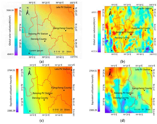
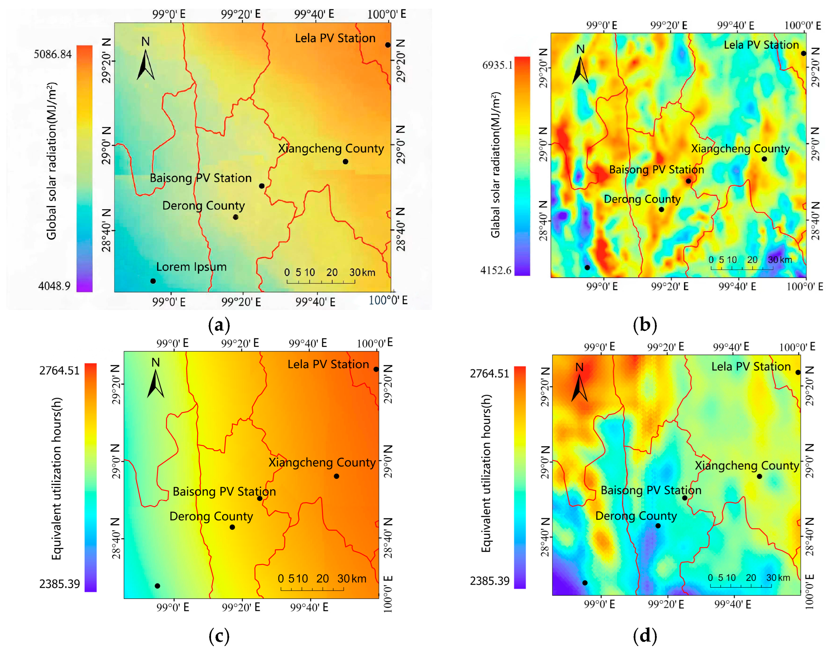
This study utilizes the 2016–2020 satellite remote sensing solar radiation data from the National Solar Radiation Database (NSRDB) (spatial resolution: 2 km × 2 km; temporal resolution: 1 h) as the observational baseline to perform bias correction and spatial downscaling on the solar radiation data output by the CMCC-ESM2 model under the CMIP6 initiative. Figure 1 shows the predicted solar radiation data for the Shuoku River Basin over the next 30 years. The multi-year total average solar radiation value for the Lela Photovoltaic Power Station area is 6574 MJ/m², while that for the Baisong Photovoltaic Power Station area is 6730 MJ/m²; both values are in good agreement with the reference data (in this study, NSRDB satellite data is used as the actual reference data). Furthermore, the multi-year average effective sunshine hours for the two power stations amount to 2658 h and 2574.5 h, respectively—both exceeding 4 h/day—and thus meet the power generation requirements of the photovoltaic power stations.

Figure 1. Thirty-year average total radiation and sunshine duration in the Shuoku River Basin. (a) Un-downscaled average total radiation. (b) Downscaled average total radiation. (c) Un-downscaled average sunshine hours. (d) Downscaled average sunshine hours.

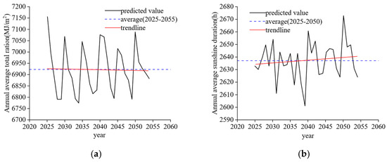
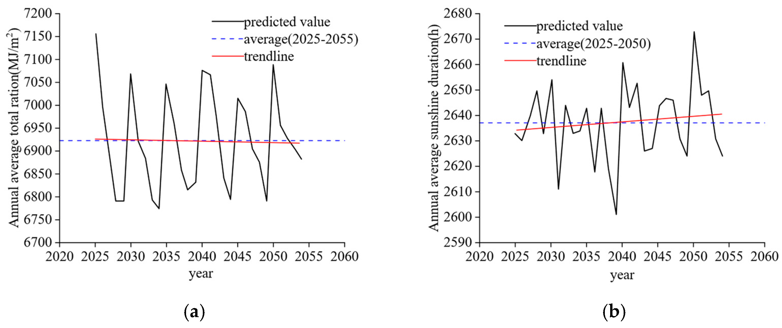
Figure 2 shows the annual average total solar radiation and sunshine duration for the Shuoku River Basin from 2025 to 2054. As shown in Figure 2a, the annual average total solar radiation ranges between 6750 MJ/m² and 7200 MJ/m²; this annual average solar radiation exhibits an oscillatory variation pattern, with the maximum amplitude occurring between 2049 and 2050 (approximately 300 MJ/m²). Overall, the annual average total solar radiation shows a slight downward trend. Figure 2b indicates that the maximum sunshine duration over the next 30 years is 2673 h, occurring in 2050, while the minimum sunshine duration is 2601.3 h, occurring in 2039. The results indicate that the average total solar radiation for the Shuoku River Basin over the next 30 years will be 6920 MJ/m², and the average effective sunshine duration will be 2637 h. This region is classified as having the “most abundant” solar resources and a “very stable” resource stability rating, providing a reliable resource base for long-term hydropower–photovoltaic complementary capacity planning and annual water allocation.

Figure 2. Predicted results for the Shuoku River Basin (2025–2054). (a) Annual average total radiation map. (b) Annual sunshine hours chart.

3.2.2. Short-to-Medium-Term Forecast

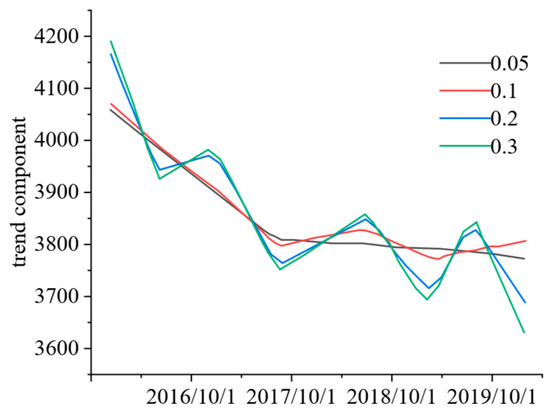
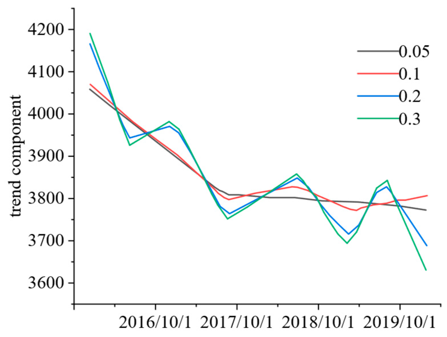
The model order determination and training were performed using the daily average solar radiation data from 2016 to 2019; the optimal GHI forecasting model was identified through BIC matrix search as ARIMA(1,1,1) (where BIC is minimized at p = 1 and q = 1, with a value of 21,461.89). Table 3 presents the BIC values calculated for various parameter combinations; for runoff forecasting, due to the stronger non-stationarity of the time series (ADF test p = 0.342, p < 0.01 after first-order differencing) and more complex temporal dependencies, the optimal model order was ARIMA(2,1,2). The trend flexibility parameter of the Prophet model was adjusted from 0.2 to 0.3 to accommodate more frequent trend turning points; Figure 3 illustrates the impact of different flexibility levels on the trend component. The annual Fourier order was reduced from 10 to 8 to prevent overfitting to the interannual variability of runoff.

Table 3. BIC matrix for the GHI sequence after first-order differencing.

	q	0	1	2	3
p
0		21,885.10	21,473.27	21,463.91	21,467.49
1		21,641.43	21,461.89	21,468.83	21,473.83
2		21,573.13	21,468.37	21,474.66	21,480.78
3		21,517.23	21,474.51	21,481.42	21,487.92

Figure 3. Impact of varying flexibility on the trend component.

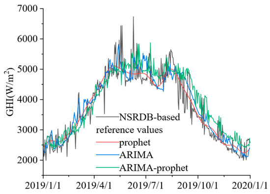
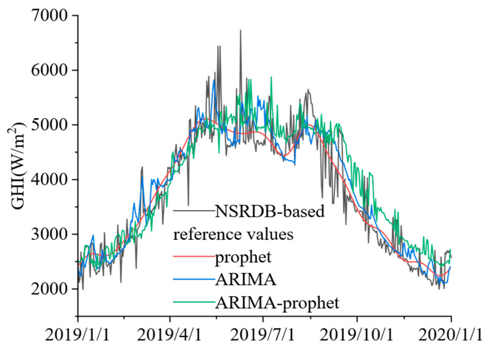
The solar radiation prediction map is shown in Figure 4; the ARIMA weight for the fusion model is 0.51 and the Prophet weight is 0.49. The ARIMA–Prophet fusion model achieved a 3.86% reduction in RMSE compared to the standalone Prophet model, indicating that the fusion model exhibits certain error reduction under these specific evaluation conditions, which validates the effectiveness of combining ARIMA’s linear trend extraction with Prophet’s periodic decomposition.

Figure 4. ARIMA–Prophet solar radiation value prediction data.

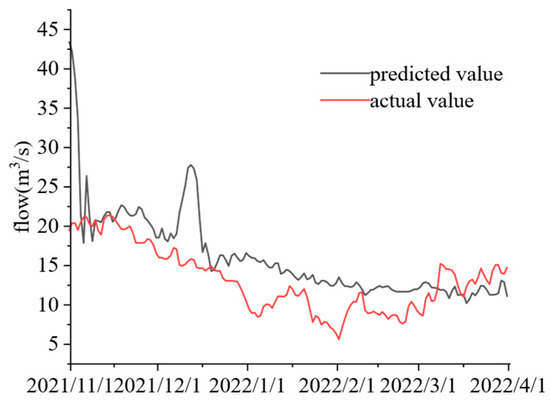
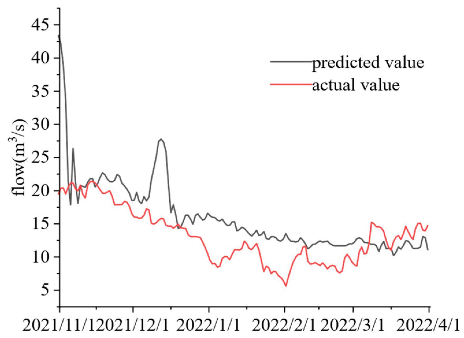
The runoff forecasting plot is shown in Figure 5; in this model, the weights assigned to the ARIMA and Prophet models each equal 0.5. A rolling forecasting validation was conducted for the dry season (from 15 November 2021, to 15 March 2022)—the period of particular interest for hydro–photovoltaic complementary scheduling—yielding a mean absolute percentage error (MAPE) of 30.53%, an average error (ME) of +2.9 m³/s, and a root mean square error (RMSE) of 8.68 m³/s. During the low-flow validation period examined in this study, the fusion model achieved the aforementioned error levels and demonstrated certain predictive capabilities; however, significant systematic bias and random errors remained. The prediction results are used for resource characteristic analysis; long-, medium-and short-term scheduling optimization employs actual observational data from corresponding historical time periods for retrospective optimization.

Figure 5. ARIMA–Prophet runoff data forecast values.

3.3. Results of the Single-Stage Multi-Time-Scale Multi-Objective Optimization Scheduling Model

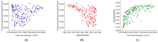
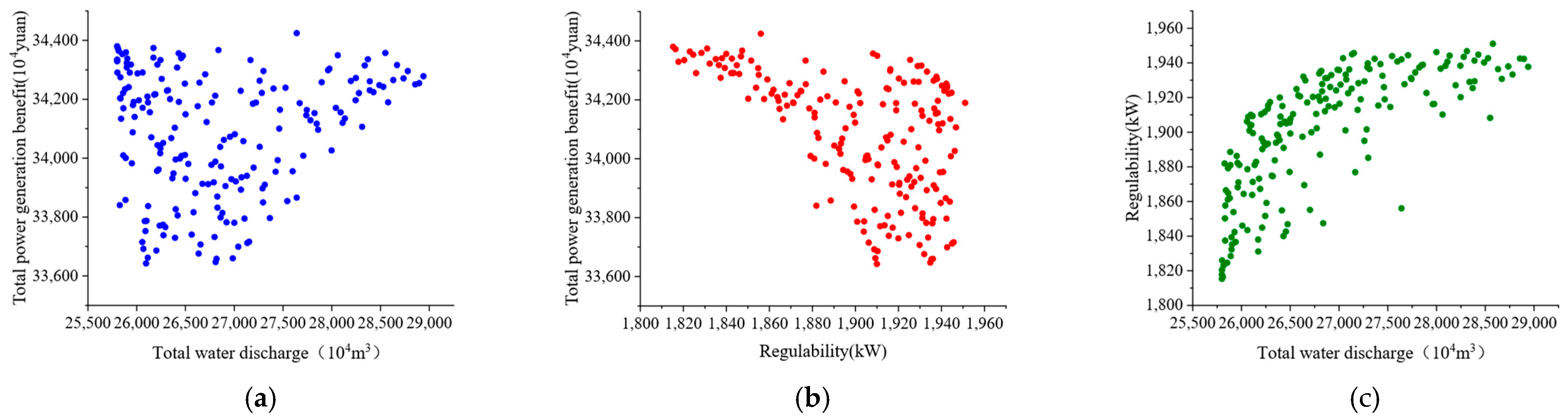
Figure 6 shows the projection of the Pareto distribution generated by the NSGA-II algorithm across the dimensions of spilled water volume, benefit, and adjustability; the Pareto front distribution is relatively uniform and distinctly characterized, with a negative correlation observed between each pair of the three optimization objectives. Notably, the total power generation benefit of multiple non-dominated solutions obtained using the NSGA-II algorithm exceeds RMB 3.024 × 10⁸, yet the corresponding spilled water volume does not increase significantly.

Figure 6. Pareto distribution of the NSGA-II algorithm. (a) Pareto distribution of total power generation benefit; (b) Pareto distribution of total power generation benefit and regulability; (c) Pareto distribution of total abandoned water volume and regulability.

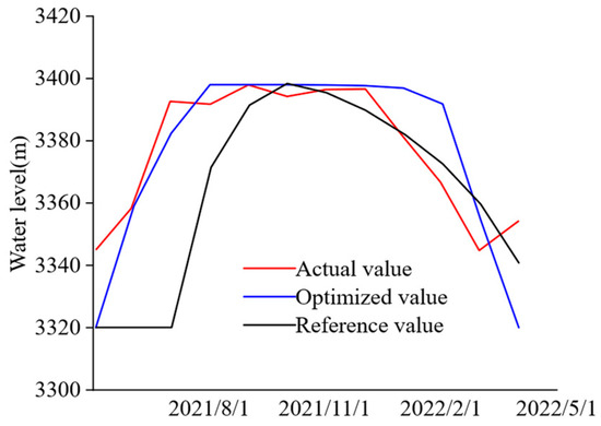
Figure 7 illustrates the annual water level allocation determined using the NSGA-II algorithm. Overall, the monthly water levels obtained via the NSGA-II algorithm enable the reservoir to maintain higher water levels for a longer duration; during the wet season (June–October), when upstream inflow increases, the reservoir fills from its lowest to its highest water level. Compared to the actual operating curve, after implementing the water–photovoltaic complementary generation strategy, the rate of water level rise accelerates, allowing the reservoir to reach the optimal power generation water level more quickly. From November to May of the following year, the period corresponds to the average-water and dry-water seasons, during which, upstream inflow decreases, and relying solely on upstream flow for power generation can no longer meet demand. Consequently, the water level values for the period from January to April of the following year in the actual operating curve exhibit a clear downward trend, attributable to the consumption of reservoir storage water to supplement the power generation flow. Under the optimized water–photovoltaic complementary generation mode, the demand for power generation at the hydropower station is reduced thanks to the supplementation provided by photovoltaic power generation; however, the utilization of upstream flow still meets the power generation requirements, thereby minimizing the consumption of reservoir storage water and enabling the reservoir to maintain a high water level for an extended period.

Figure 7. Long-term optimization results for single-stage water–photovoltaic complementary system (water level).

According to Table 4, for both power generation output and revenue generation, the unoptimized annual power generation under the water–photovoltaic complementary generation approach amounts to 994 million kWh, with energy-equivalent hydropower curtailment loss of 278 million kWh; after optimization using the NSGA-II algorithm, the annual power generation reaches 1057 million kWh, with an energy-equivalent hydropower curtailment loss of 164 million kWh. Compared to the unoptimized scenario, the power generation output increases by 6.34%, energy-equivalent hydropower curtailment loss is reduced by 41.01%, and the power generation revenue rises by RMB 4,958,300.

Table 4. Long-term optimization results for single-stage water–photovoltaic complementary energy system.

Month	Water Level (m)	Inlet Flow Rate (m3/s)	Power Generation Flow Rate (m3/s)	Discharge (m3/s)	Output of Power Station (MW)	Photovoltaic Output (MW)	Monthly Income (Wan Yuan)	Adjustability (MW)
6	3320.00	49.89	45.49	0.00	90.17	32.01	2499.25	50.00
7	3358.99	109.26	80.79	0.00	164.02	23.90	3987.48	50.00
8	3382.42	208.91	78.23	96.26	179.48	25.92	4358.48	114.98
9	3398.00	106.37	71.88	0.07	182.49	22.91	4219.62	156.86
10	3398.00	38.41	34.01	0.00	95.50	23.97	2529.70	201.00
11	3398.00	23.44	19.04	0.00	55.35	17.77	1856.64	201.00
12	3397.91	9.95	5.74	0.00	19.82	16.39	1030.51	201.00
1	3397.69	9.95	6.00	0.00	20.50	36.00	1460.44	200.74
2	3396.91	9.08	6.48	0.00	21.75	37.64	1389.15	200.13
3	3391.81	9.49	15.27	0.00	44.83	40.64	2404.90	197.92
4	3354.91	14.83	62.56	0.00	150.91	29.19	5679.05	183.47
5	3320.00	22.63	38.49	0.00	82.69	31.30	2964.71	108.18

Notes: The entry “output of power station (MW)” in Table 4 corresponds to the monthly average hydroelectric power output derived from long-term monthly scale calculations.

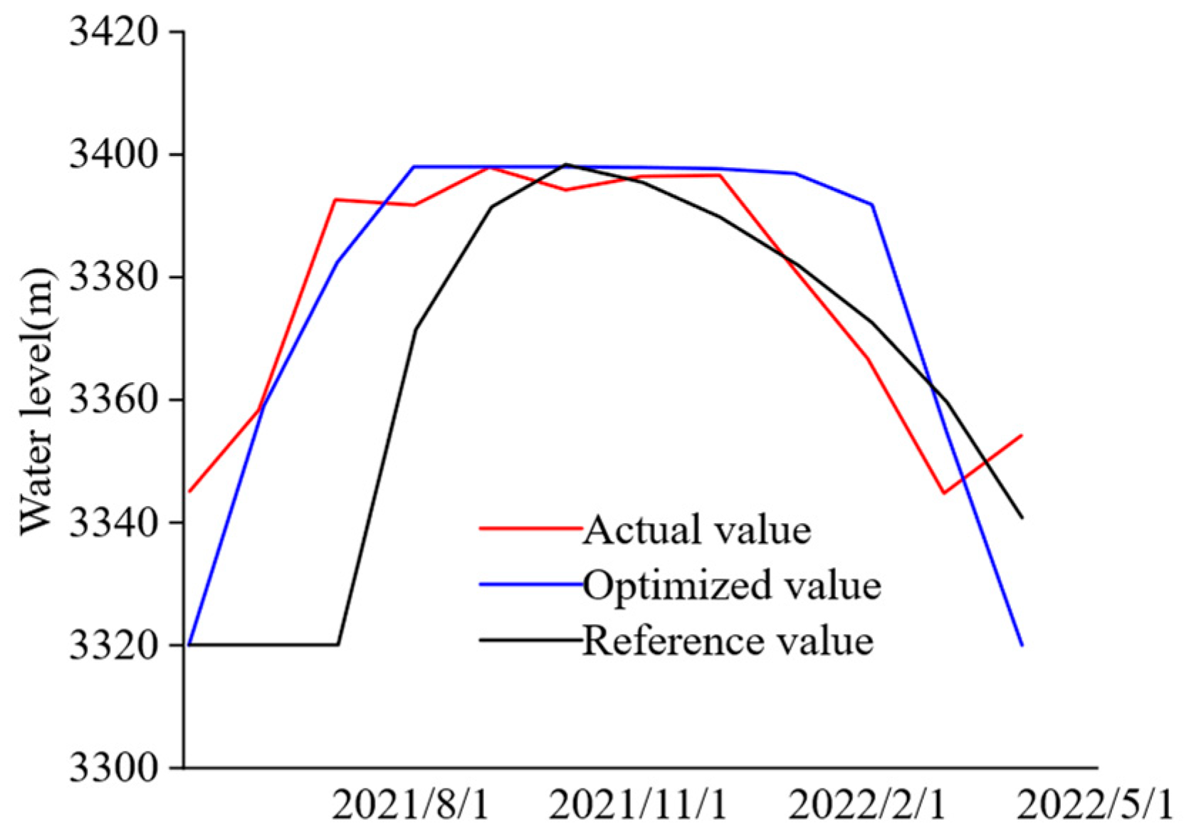
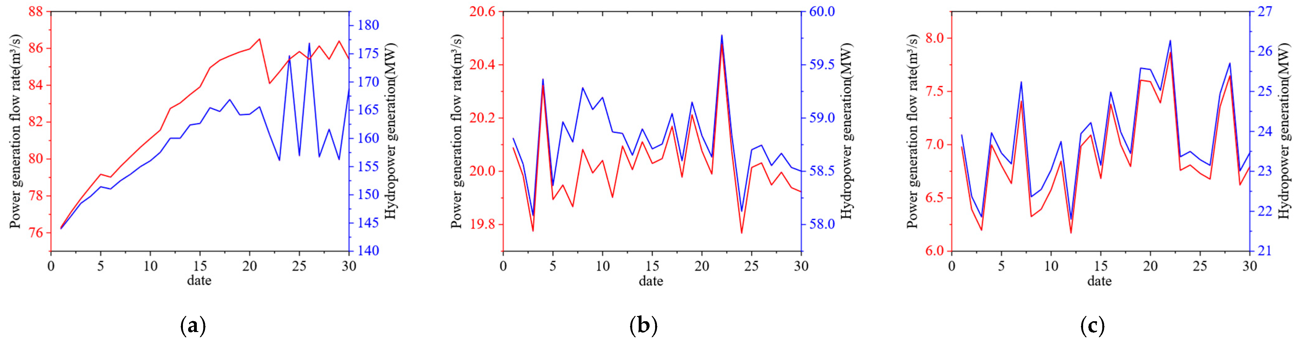
In the mid-term hydro–solar complementary energy system optimization study, the problem of daily water usage allocation over a one-month period was investigated. Given the significant seasonal variations in both photovoltaic power output and upstream water flow, three representative months—July (high-water period), November (average-water period), and January (low-water period)—were selected to analyze the optimal operational outcomes for the hydro–solar complementary system. Figure 8 illustrates the mid-term optimal optimization results obtained using the NSGA-II algorithm; the water level variation trends for each month reflect the influence of the distinct inflow characteristics associated with the high-and low-water periods. Figure 8a presents the optimization results for the flood season in July 2023. The power generation flow rate exhibits a significant positive correlation and synergistic variation with the total hydropower output; the power generation flow rate gradually increased from 76.22 m³/s on day 1 to 79.89 m³/s on day 31, while the hydropower output during the same period rose from 144.21 MW to 178.22 MW. Although the trends of the two variables were consistent, the increase in hydropower output was more pronounced. This phenomenon occurred because, during the flood season, reservoirs began to be filled, leading to a continuous increase in the hydraulic head, which in turn increased the power output per unit of power generation flow rate. Compared to the actual power generation process, the total monthly power generation during the flood season increased by 12.8022 million kW·h, and the monthly power generation efficiency improvements increased by an average of 11.45%. Figure 8b shows the optimization results for the normal season. In this phase, the upstream inflow generally sufficed to meet power generation demands; consequently, the water levels at the end and beginning of the month differed little, the hydraulic head remained largely consistent, and a significant linear relationship existed between the power generation flow rate and the total hydropower output. Compared to the actual power generation process, the monthly power generation during the normal season decreased by 4.287 million kW·h; this reduction was attributed to the practice of utilizing additional reservoir capacity to generate extra electricity during that month, which resulted in a decrease in the water level by 0.78 m at the end of the month and a reduction in reservoir capacity by 4.47 million m³. Figure 8c displays the optimization results for the dry season. In this phase, the upstream inflow was insufficient to meet power generation demands, necessitating the depletion of reservoir capacity; both the power generation flow rate and the total hydropower output were significantly lower than those observed during the flood and normal seasons, respectively.

Figure 8. Mid-term optimization results for a single-stage water–photovoltaic complementary system: (a) wet season; (b) normal water level period; (c) low water period.

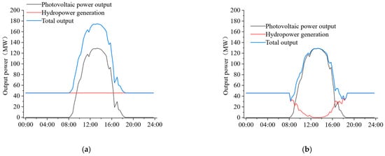
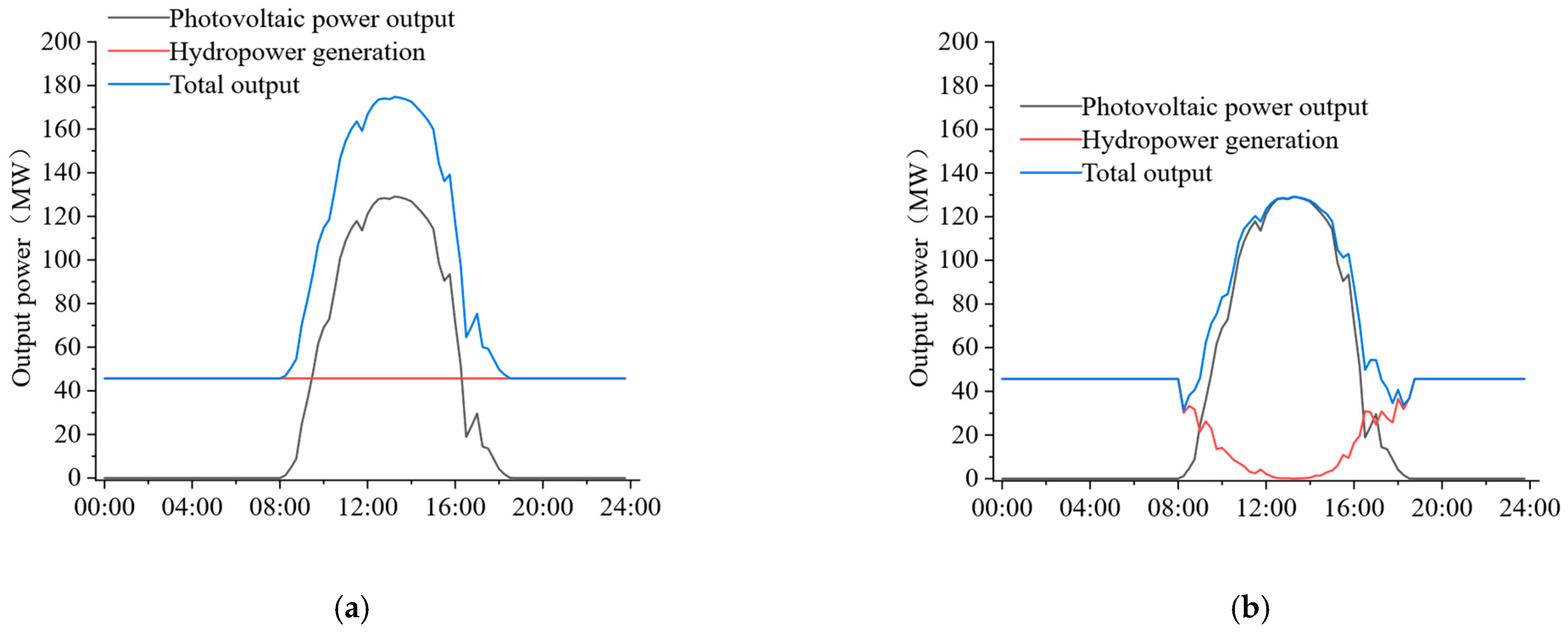
Figure 9b illustrates the short-term optimization results of the hydropower–solar complementary system for the dry season on 1 January 2024. The solar power output exhibits distinct diurnal fluctuations: it gradually increases from 8:00 a.m. (sunrise), reaches its peak value of 129.13 MW at 12:00 p.m., then progressively declines, and drops to zero after 6:00 p.m. To mitigate the intermittency and volatility of solar power output, during nighttime and early morning hours—when solar output is zero—hydropower output is maintained at a relatively high level (45.68 MW) to fulfill the base load requirement; conversely, during peak solar output periods (8:00 a.m. to 4:00 p.m.), hydropower output is correspondingly reduced, thereby helping to smooth overall power output fluctuations to a certain extent. The total power output fluctuates cyclically within the range of 45–129 MW, resulting in an overall smooth power profile. However, due to the limited available water supply for the day, complete smooth integration of solar power output cannot be achieved; consequently, the total power output exhibits a pronounced increase during solar power generation periods. The standard deviation of the total treated power before optimization was 48.510 MW, while after optimization, it was 31.536 MW. This dispatch strategy fully leverages the rapid regulation capability of hydropower, achieving relatively smooth overall system power output and demonstrating the feasibility of hydropower–solar complementarity on short-term time scales.

Figure 9. Short-term optimization results for single-stage water–photovoltaic complementary energy system. (a) Pre-optimization of photovoltaic and hydropower output; (b) optimized photovoltaic and hydroelectric power output.

3.4. Discussion

Compared with previous studies on hydro–PV complementary operation, the proposed framework is characterized by an explicit hierarchical organization of long-, medium-, and short-term scheduling decisions. Zhang et al. [5] integrated long-term and short-term hydro-PV operational modes mainly for photovoltaic capacity planning and analyzed the effects of hydropower discharge constraints on photovoltaic curtailment. Yuan et al. [6] incorporated short-term operational performance into long-term scheduling through auxiliary scheduling functions, thereby improving the coordination between long-term generation and short-term operation. Shen et al. [13] further developed a multi-time-scale scheduling framework considering the spatiotemporal correlation between hydropower and photovoltaic resources, while Cheng et al. [16] proposed a synchronized framework covering short-, medium-, and long-term operations of hydro–wind–PV complementary systems. These studies demonstrate the importance of cross-timescale coordination in hybrid renewable energy scheduling. The present study extends this research line by integrating three components into a unified framework: complementary resource assessment, multi-time-scale resource forecasting, and hierarchical multi-time-scale optimization. Specifically, long-term scheduling determines inter-period water allocation and generation boundaries, medium-term scheduling refines daily water-use allocation within these boundaries, and short-term scheduling performs 15 min scale compensation of photovoltaic fluctuations. The coupling among the three layers is achieved through the transfer of reservoir water levels, water-use boundaries, and generation targets. Therefore, the contribution of this study can be understood primarily as the integration and physical coordination of complementary assessment, forecasting, and hierarchical scheduling.

This study focuses on a single cascade power station (Gua Wa Power Station) as its primary subject; however, it has not yet fully accounted for the coordinated regulation capability among multiple cascades nor the impact of varying physical characteristics on the selection of decision variables. Additionally, there is significant room for improving the accuracy of the ARIMA–Prophet fusion model in runoff forecasting. Future research could extend this methodology to cascade hydropower–photovoltaic complementary systems and integrate factors such as electricity market mechanisms and demand response to further refine a multi-time-scale collaborative optimal dispatch framework, thereby providing more comprehensive technical support for the safe and stable operation of power systems under high penetration of renewable energy sources.

4. Conclusions

This paper addresses the operational optimization problem of hydro–photovoltaic complementary power systems under high penetration of renewable energy sources. Taking the Guwa–Lela hydro–photovoltaic complementary power system along the Shuoku River as a case study, the paper proposes a multi-time-scale dispatching method centered on the concept of “hydro-regulated photovoltaic generation.” A integrated research framework encompassing “resource assessment–resource forecasting–multi-time-scale optimization” is established. The main findings of this study are as follows:

(1) In the context of evaluating the complementarity between hydropower and solar energy systems, the six-dimensional comprehensive evaluation indicator system developed in this study enables an effective assessment of the complementary potential of water and solar resources within a river basin. The results obtained using the Analytic Hierarchy Process (AHP) demonstrate that the Regulation Capability Index plays a significant role in the complementarity evaluation, confirming that the reservoir’s regulation capability is a core parameter for hydropower–solar complementary systems and providing a theoretical foundation for subsequent dispatch strategies centered on hydropower regulation.

(2) For hydro–photovoltaic resource forecasting, the long-term forecast employs the quantile mapping method to calibrate and spatially downscale the CMIP6 model output data, increasing the resolution to 2 km × 2 km. The forecast indicates that the average total solar radiation over the watershed for the next 30 years will be 6920 MJ/m². For medium-to-short-term forecasting, an ARIMA–Prophet fusion model was developed; this model effectively integrates linear trends through feedback inverse weighting, enhancing its periodicity and decomposition capabilities and indicating a certain reduction in prediction error under the specific evaluation environment. Under typical low-water-year conditions, the MAPE for runoff forecasting is 30.53%, offering a usable resource input for medium-to-short-term scheduling.

(3) For multi-time-scale planning and optimal scheduling, this study proposes a long-, medium-, and short-term multi-objective optimization framework. The framework establishes interconnections across different time scales through grid-connected power balance relationships and employs the NSGA-II algorithm to perform multi-objective optimization of power generation and resource utilization efficiency. The results demonstrate that, after long-term optimization, power generation increased by 6.34% compared to the baseline scenario, hydroelectric curtailment losses were reduced by 41.01%, and power generation revenue rose by RMB 4,958,300; medium-term optimization achieved monthly power generation efficiency improvements of 11.45% during the high-water periods; and through the rapid complementary regulation of photovoltaic generation by hydropower output, the daily output power fluctuates cyclically between 45 and 129 MW, while the overall output remains smooth, thereby validating the feasibility of the “hydro-regulated photovoltaic generation” strategy for real-time mitigation of photovoltaic output fluctuations. This method is applicable to water–solar complementary systems similar to the Guwa–Lela system—specifically those equipped with reservoir regulation capabilities and capable of coordinating water resource allocation with photovoltaic power fluctuation compensation across multiple time scales; however, further extension and validation are required for applications involving multi-reservoir cascaded coordination, stochastic uncertainty optimization, and cross-regional deployment under diverse resource conditions.

References

- Dong, W.; Zhang, J.; Zhou, Q.; Zhang, L.; Gong, H. A Review of the Evolution of Power System Security and Stability in China. China Electr. Power 2025, 58, 115–127. [Google Scholar] [CrossRef]
- Glasnovic, Z.; Margeta, J. The features of sustainable solar hydroelectric power plant. Renew. Energy 2009, 34, 1742–1751. [Google Scholar] [CrossRef] [Scilit]
- Zhao, M.; Wang, Y.; Wang, X.; Chang, J.; Chen, Y.; Zhou, Y.; Guo, A. Flexibility evaluation of wind-PV-hydro multi-energy complementary base considering the compensation ability of cascade hydropower stations. Appl. Energy 2022, 315, 119024. [Google Scholar] [CrossRef] [Scilit]
- Zhang, Y.; Ma, C.; Lian, J.; Pang, X.; Qiao, Y.; Chaima, E. Optimal photovoltaic capacity of large-scale hydro-photovoltaic complementary systems considering electricity delivery demand and reservoir characteristics. Energy Convers. Manag. 2019, 195, 597–608. [Google Scholar] [CrossRef] [Scilit]
- Zhang, J.; Guo, A.; Wang, Y.; Chang, J.; Wang, X.; Wang, Z.; Tian, Y.; Jing, Z.; Peng, Z. How to achieve optimal photovoltaic plant capacity in hydro-photovoltaic complementary systems: Fully coupling long-term and short-term operational modes of cascade hydropower plants. Energy 2024, 313, 134161. [Google Scholar] [CrossRef] [Scilit]
- Yuan, W.; Sun, Z. Long-Term Optimal Scheduling of Hydro-Photovoltaic Hybrid Systems Considering Short-Term Operation Performance. Energies 2024, 17, 5388. [Google Scholar] [CrossRef] [Scilit]
- Huang, K.; Liu, P.; Ming, B.; Kim, J.-S.; Gong, Y. Economic operation of a wind-solar-hydro complementary system considering risks of output shortage, power curtailment and spilled water. Appl. Energy 2021, 290, 116805. [Google Scholar] [CrossRef] [Scilit]
- Guo, Y.; Ming, B.; Huang, Q.; Wang, Y.; Zheng, X.; Zhang, W. Risk-averse day-ahead generation scheduling of hydro–wind–photovoltaic complementary systems considering the steady requirement of power delivery. Appl. Energy 2022, 309, 118467. [Google Scholar] [CrossRef] [Scilit]
- Lu, N.; Wang, G.; Su, C.; Ren, Z.; Peng, X.; Sui, Q. Medium-and long-term interval optimal scheduling of cascade hydropower-photovoltaic complementary systems considering multiple uncertainties. Appl. Energy 2024, 353, 122085. [Google Scholar] [CrossRef] [Scilit]
- Su, C.; Li, L.; Zhang, T.; Sui, Q.; Yang, Y. A real-time scheduling framework of cascade hydropower-photovoltaic power complementary systems based on model predictive control. Appl. Energy 2025, 392, 126023. [Google Scholar] [CrossRef] [Scilit]
- Zhu, F.; Zhong, P.-A.; Sun, Y.; Xu, B.; Ma, Y.; Liu, W.; Zhang, D.; Dawa, J. A coordinated optimization framework for long-term complementary operation of a large-scale hydro-photovoltaic hybrid system: Nonlinear modeling, multi-objective optimization and robust decision-making. Energy Convers. Manag. 2020, 226, 113543. [Google Scholar] [CrossRef] [Scilit]
- Xu, S.; Liu, P.; Li, X.; Cheng, Q.; Liu, Z. Deriving long-term operating rules of the hydro-wind-PV hybrid energy system considering electricity price. Renew. Energy 2023, 219, 119353. [Google Scholar] [CrossRef] [Scilit]
- Wan, Y.; Shen, L.; Wang, Q.; Xu, X.; Liu, Y. Multi-timescale scheduling optimization of cascade hydro-solar complementary power stations considering spatio-temporal correlation. Sci. Technol. Energy Transit. 2025, 80, 17. [Google Scholar] [CrossRef] [Scilit]
- Cheng, Q.; Liu, P.; Feng, M.; Cheng, L.; Ming, B.; Xie, K.; Yang, Z.; Zhang, X.; Zheng, Y.; Ye, H. Leveraging a deep learning model to improve mid-and long-term operations of hydro-wind-photovoltaic complementary systems. Renew. Sustain. Energy Rev. 2025, 222, 115986. [Google Scholar] [CrossRef] [Scilit]
- Liu, B.; Liu, T.; Liao, S.; Lu, J.; Cheng, C. Short-term coordinated hybrid hydro-wind-solar optimal scheduling model considering multistage section restrictions. Renew. Energy 2023, 217, 119160. [Google Scholar] [CrossRef] [Scilit]
- Cheng, Q.; Liu, P.; Ming, B.; Yang, Z.; Cheng, L.; Liu, Z.; Huang, K.; Xu, W.; Gong, L. Synchronizing short-, mid-, and long-term operations of hydro-wind-photovoltaic complementary systems. Energy 2024, 305, 132309. [Google Scholar] [CrossRef] [Scilit]
- Fan, Y.; Zhong, P.; Zhu, F.; Mo, R.; Wang, H.; Wei, J.; Zeng, Y.; Wang, B.; Qian, X. Assessing the potential and complementary characteristics of China’s solar and wind energy under climate change. Renew. Energy 2025, 249, 123213. [Google Scholar] [CrossRef] [Scilit]
- Xian, Y.; Wang, T.; Leng, W.; Letu, H.; Shi, J.; Wang, G.; Yan, X.; Yuan, H. Can topographic effects on solar radiation be ignored: Evidence from the Tibetan Plateau. Geophys. Res. Lett. 2024, 51, e2024GL108653. [Google Scholar] [CrossRef] [Scilit]
- Hua, K.; Wang, Z.; Yao, Y.; Jiang, G.; Han, L.; Wan, J.; Tian, D.; Yang, D. Fine-grained solar energy distribution assessment and long-term forecasting based on the quantile mapping method. J. China Univ. Pet. (Nat. Sci. Ed.) 2024, 48, 198–205. [Google Scholar]
- Baloch, M.; Honnurvali, M.S.; Kabbani, A.; Jumani, T.A.; Chauhdary, S.T. An intelligent SARIMAX-based machine learning framework for long-term solar irradiance forecasting at Muscat, Oman. Energies 2024, 17, 6118. [Google Scholar] [CrossRef] [Scilit]
- Saidani, K.; Essaddi, N.; Besbes, M. Harnessing Prophet Model with Rigorous Cross Validation For Long term Solar Insolation Prediction. Results Eng. 2025, 28, 107915. [Google Scholar] [CrossRef] [Scilit]
- Ssekulima, E.B.; Etemadi, A.H. Stochastic optimization framework for capacity planning of hybrid solar PV–small hydropower systems using metaheuristic algorithms. Complex Intell. Syst. 2026, 12, 32. [Google Scholar] [CrossRef] [Scilit]
- Gao, J.; Lin, T.; He, X.; Bai, J.; Yuan, L. Fuzzy comprehensive evaluation of mini pumped hydro storage based on combined weighting method. J. Energy Storage 2026, 152, 120734. [Google Scholar] [CrossRef] [Scilit]
Disclaimer/Publisher’s Note: The statements, opinions and data contained in all publications are solely those of the individual author(s) and contributor(s) and not of MDPI and/or the editor(s). MDPI and/or the editor(s) disclaim responsibility for any injury to people or property resulting from any ideas, methods, instructions or products referred to in the content. |
© 2026 by the authors. Licensee MDPI, Basel, Switzerland. This article is an open access article distributed under the terms and conditions of the Creative Commons Attribution (CC BY) license.