


Abstract
Assessing additional converter capacity requires stability analysis under operating, control, device-model and network-topology uncertainty. This paper integrates structured singular value analysis with branch and bound to assess regions in engineering coordinates, including capacity, short-circuit ratio, synchronisation bandwidth and reactive support. Each box undergoes equilibrium screening and structured uncertainty analysis; candidate instability is confirmed by reconstructing a physical scenario and applying a winding-number test. On a nine-bus, six-device system, the computation assigns 8.34% of the domain to verified robust boxes, 38.80% to undecided boxes, 18.49% to boxes containing confirmed instability witnesses and 34.37% to boxes rejected by equilibrium screening. Verification on a 44-point frequency grid reduces the initial robust share from 19.01% to 8.34%. Under a fixed stressed scenario, the critical capacity is bracketed between 477.148 and 477.178 MW. An average-value electromagnetic-transient model reproduces the candidate device’s positive-rotation admittance with deviations of approximately 0.2% in magnitude and 0.2° in phase at eight frequencies, as well as the strongly unstable system growth rate to about 2%; switching simulations corroborate selected qualitative outcomes. The contribution is the integrated planning workflow. Its reported coverage depends on refinement and identification quality and remains conditional on sampled equilibrium and residual assessments and finite-frequency evaluation.
1. Introduction
The Introduction identifies the planning problem, reviews the relevant modelling and robustness methods, and defines the scope of the proposed workflow.
1.1. Motivation
Transmission corridors that were designed around synchronous generation are being replanned around converter-interfaced resources. When a planner is asked whether a further block of wind, photovoltaic or storage capacity can be connected at a given bus, the answer is no longer delivered by a thermal or voltage check alone. Grid-following (GFL) converters synchronise through a phase-locked loop (PLL); impedance-based studies have shown that PLL interaction with a weak grid of finite short-circuit capacity can produce low-frequency oscillatory instability [1,2]. The admissible limit depends jointly on the capacity to be added, strength of the network behind the point of common coupling, bandwidth of the synchronisation loop, and reactive support installed nearby. These four quantities are collected in this paper as the engineering coordinate vector; Section 2 establishes why an answer must be expressed in exactly these coordinates to be usable by the process that needs it.
The practical difficulty is that nothing else surrounding the decision is known exactly. The operating point migrates with resource availability and load; for a plant that has not yet been procured, controller gains and bandwidths are available to the planner as specified tolerances rather than as identified values, which motivates their treatment as bounded uncertainty [3,4]; the terminal behaviour of a vendor-supplied converter is disclosed only up to an identification envelope, because its internal control is proprietary; and the network must remain admissible under a set of credible topology changes. The honest form of the planning question is, therefore, set-valued: for which engineering coordinate vector does the corridor remain small-signal stable for every operating deviation, every control tolerance, every port model within its envelope, and every credible topology?
Point-wise scanning, which is the prevailing practice, cannot answer a question of this form. A scan evaluates a stability test at finitely many sampled parameter vectors and returns verdicts at those vectors only; the continuum between the samples remains unexamined, and it is exactly there that a connection capacity must be committed. Nor can the deficiency be repaired by density alone: small-signal stability is not a monotone function of the parameters in converter-dominated networks, so interpolation between two stable samples is not a valid inference. A scan can supply a counterexample, which is genuinely useful, but it cannot supply a certificate. What the planner needs is the inverted logic—a bound that holds over an entire sub-box of parameters at once, together with an explicit statement of where that bound stops being conclusive.
A region-valued answer, moreover, must distinguish outcomes that carry different engineering consequences—standing approval, targeted remedy, network reinforcement, or further study—because collapsing them into a binary verdict discards the information that makes the answer actionable; the four-class partition that formalises this distinction and the planning consequence attached to each class are developed in Section 2.3.
EMT comparisons examine whether selected analytic predictions are reproduced by time-domain models. The average-value layer supports quantitative admittance and growth-rate comparisons, while the switching layer tests qualitative outcomes with a realistic sampled implementation. These comparisons are a validation component of the workflow, not proof that the complete physical uncertainty family is enclosed.
1.2. Related Work
Impedance-based analysis supplies the modelling foundation. Sun formalised the impedance-ratio Nyquist criterion for a source–load interconnection and showed that the stability of a converter–grid interface can be assessed from terminal characteristics alone [5]; the formulation is well suited to proprietary equipment, but it is stated for a single interface and evaluates one parameter point at a time, so it yields no region in a planning space. Harnefors et al. derived the input admittance of controlled voltage-source converters and showed how the control structure shapes it towards or away from passivity [6]; the dissipation viewpoint explains the destabilising mechanism, yet passivity-based shaping presumes access to the converter internals that a planner facing vendor equipment does not have, and the assessment remains point-wise in the parameters. Cespedes and Sun constructed analytical three-phase converter impedance models including the PLL and the current control and validated them against measurement [7]; their comparison makes visible the very quantity a nominal criterion cannot absorb—the band between the measured and the modelled response—which is exactly the envelope information that the present framework promotes into the certificate itself.
The dq-frame refinement of these models exposed the multivariable structure of the problem. Wen et al. derived the two-by-two dq impedance of grid-tied inverters and identified the PLL-induced negative-resistance behaviour of the q-axis channel [1]; the multivariable coupling they demonstrated is the reason a scalar impedance ratio does not suffice, and it motivates the structured, matrix-valued uncertainty description adopted here—but the analysis itself is a nominal-case assessment. Dong et al. analysed the low-frequency interaction between the PLL and a weak grid and quantified how the admissible synchronisation bandwidth contracts as the short-circuit ratio falls [2]; the study isolates the trade-off that dominates the present test system, yet it delivers a boundary curve for a nominal single converter, not a certified interval for a multi-device corridor.
Aggregation to the system level has been addressed through whole-system admittance models. Gu et al. embedded the local reference-frame dynamics of heterogeneous devices into one whole-system impedance model and showed that the construction scales to composite grids [8]; the nodal formulation is adopted in this paper, but the published studies evaluate it at nominal parameters, so the set-valued question is not posed. Zhu et al. developed grey-box participation analysis, locating which converters and which internal parameters drive a given whole-system mode without requiring full control disclosure [9]; participation tells the analyst where uncertainty matters, which is complementary to—but different from—bounding how much uncertainty is tolerable, which is the question a certificate must answer.
The interaction of device classes sharpens the problem further. Li et al. unified grid-forming (GFM) and grid-following operations through a duality theory that explains their complementary synchronisation behaviour [10]; the insight is structural and guides the device templates used here, but it does not by itself produce a quantitative admissible region. Xin et al. asked how many grid-forming converters a system needs and answered it through generalised grid-strength metrics [11]; the study quantifies the GFM/GFL mix at the planning level, yet its conclusions rest on nominal models and sampled evaluations, so the space between evaluated configurations carries no guarantee, and continuous control and model-error uncertainty is not carried inside the metric.
The planning literature poses the capacity question directly. Yuan et al. computed the maximal admissible GFL capacity under grid-strength constraints [3]; this is the same engineering question addressed here, but stability enters through aggregate strength proxies rather than as a certified small-signal condition, and device model error has no place in the formulation. Zhang et al. characterised renewable hosting capacity as a feasible region with an explicit frequency-security constraint [12]; the output is region-valued, which is the right form, but the dynamic constraint is the frequency nadir rather than oscillatory small-signal stability, and no worst-case guarantee is attached to the interior of the region.
Robust control theory supplies the machinery for converting a nominal criterion into a set-valued one. Doyle introduced the structured singular value μ as the exact measure of robust stability under block-structured uncertainty [13]; exactness, however, comes with intractability, and the value must be bounded. Packard and Doyle consolidated complex-μ theory—the linear-fractional machinery, the D-scaling upper bound and the power-iteration lower bound—into the computational canon [14]. Young et al. extended the bounds to mixed real and complex uncertainty through D and G scalings, making genuinely parametric blocks computable [15], and Newlin and Young combined the mixed bounds with branch and bound on the uncertainty set to close the residual gap between them [16]. This chain is the mathematical backbone of the present method, and none of it is claimed as a contribution; what the chain does not supply is the power-system construction in front of it—a sound enclosure that maps the movement of the operating point, the steady-state frame rotations, and the vendor port envelopes of a meshed multi-converter network into one admissible perturbation structure. A μ bound certifies the enclosure it is given; without a sound enclosure it certifies nothing about the physical system.
Applications of structured robustness analysis to power systems exist and delimit the state of the art. Castellanos et al. applied structured-singular-value analysis to large, interconnected power systems under parametric uncertainty [17]; the study demonstrates scale, but the uncertain dynamics are those of classical machines, and neither converter port envelopes nor planning coordinates appear. Sumsurooah et al. mapped μ analysis into explicit robust stability domains in a parameter space for a converter system with a constant-power load [4]; this is the closest prior art in spirit—a certified parametric domain—but the system is a single-converter architecture, the domain is not screened for equilibrium existence, the conservatism of the certificate is not decomposed, and no EMT cross-validation is reported. Kim et al. recently applied μ-synthesis to inverter-based resources under weak-grid impedance uncertainty [18]; the work confirms the currency of structured methods for converter-dominated grids, but it synthesises a controller for one device rather than certifying a region for a system.
On the equilibrium side, interval analysis provides the corresponding rigorous tool. Wang and Alvarado introduced interval arithmetic into power-flow analysis and obtained guaranteed solution enclosures under data uncertainty [19]; the enclosures are static statements, never coupled to a dynamic certificate. Ding et al. applied the Krawczyk operator, with a preconditioner guaranteeing convergence, to interval power flow under renewable uncertainty [20]; the existence machinery is exactly what a region determination needs, but the setting is a radial distribution feeder and the certificate stands alone. Wang et al. gave fixed-point conditions for the existence and uniqueness of the load-flow solution [21]; the conditions are analytic and elegant, yet they have not been embedded in a determination procedure in which the loss of equilibrium competes with the loss of stability as the binding constraint. Nogueira et al. demonstrated Krawczyk-contracted interval load flow in this journal [22], confirming that the tool is current; its use, again, remains detached from any small-signal question.
Finally, the validation strand: Mahseredjian et al. surveyed electromagnetic-transient simulation methods and established EMT as the reference environment in which averaged models are to be judged [23]; what the survey’s perspective makes conspicuous is how rarely set-valued stability certificates are carried down to that reference—even though the certified quantity, a modal growth rate, is exactly what an EMT run can measure. For the digital control path, the z-domain small-signal formalism and the now-standard one-and-a-half-sample computation-plus-hold delay convention were established for digitally controlled converters in [24,25]; both treat the delay as a device-level design constraint, whereas a system-level certificate must carry the delay inside every device port model and must demonstrate that its EMT realisation reproduces the certified dynamics rather than merely resembling them.
1.3. Unresolved Issues and Contributions
Five unresolved issues follow from this record. First, impedance-based criteria are mature but are evaluated at nominal parameter points, so they cannot certify an interval, which is the object a planning decision requires. Second, structured robustness tools are mature but are not connected to engineering coordinates: their inputs are abstract perturbation blocks and their outputs are margins, neither of which a planner can act upon without a construction that is absent from the theory. Third, the existence of an admissible equilibrium and the small-signal stability of that equilibrium are treated in separate bodies of literature, although in a converter-dominated corridor the binding constraint switches between them as the operating point moves, and a method that reports only a stability verdict misattributes the transfer-limited part of the domain. Fourth, the conservatism of a set-valued certificate is rarely decomposed, so it remains unknown whether tightening a device envelope, refining a partition, or improving a relaxation is the effective remedy—a question with direct budgetary consequences, since these remedies are purchased with different resources. Fifth, set-valued certificates are almost never cross-validated against switching-level EMT simulation, although the certified quantity—the growth rate of the dominant mode—is directly measurable there.
The contribution is an engineering workflow that integrates established robust-control, interval-analysis and branch-and-bound tools for multi-converter planning. No new structured-singular-value bound, winding-number criterion, Krawczyk theorem or branch-and-bound theory is claimed. The specific contributions are the following; their numerical scope is qualified in Section 3.5, Section 4.1 and Section 4.4.
- Joint uncertainty analysis in engineering coordinates. A structured linear-fractional representation combines operating and control deviations, device port envelopes and the affine-enclosure residual. Branch and bound converts the per-box assessments into a four-way partition. Each unstable label requires an independently confirmed physical counterexample, rather than a lower bound alone.
- Ordered equilibrium and stability assessment. Equilibrium screening precedes dynamic analysis, separating possible transfer limitations from oscillatory instability. The study distinguishes vertex-and-sample screening at production resolution from a rigorous interval existence certificate.
- Quantification of numerical coverage. Comparisons across identification envelopes, partition depths and frequency grids show how these choices affect the reported robust and undecided shares. The results guide the allocation of identification and computational effort within the tested configurations.
- Staged EMT comparison. An average-value model provides quantitative device-admittance and system-mode comparisons, while a switching model checks selected qualitative outcomes. The candidate-device positive-rotation admittance differs by approximately 0.2% in magnitude and 0.2° in phase at the eight tested frequencies; the strongly unstable growth rate agrees to about 2%. These tests corroborate selected model predictions, not every box of the region.
1.4. Organisation
Section 2 formulates the engineering domain and uncertainty set. Section 3 develops the device and network models and equilibrium screen. Section 4 and Section 5 describe the structured bounds and branch-and-bound classification. Section 6 presents the EMT methodology, Section 7 reports the case studies and computational effort, and Section 8 summarises the findings and limitations.
2. Problem Formulation
This section defines the engineering coordinates, the joint uncertainty set and the ideal region classes. It also distinguishes these ideal sets from the box labels obtained by the numerical procedure.
2.1. The Engineering Question and Its Coordinates
The corridor under study carries a heterogeneous fleet of synchronous machines (SG), grid-following converters (GFL), which synchronise to the network through a phase-locked loop, and grid-forming converters (GFM), which impose their own voltage phasor. A planner is asked whether a further block of grid-following capacity may be connected at a specified bus of this corridor. The question sounds like a request for a single number—a hosting capacity—and it has, indeed, been treated as one in grid-strength-constrained capacity assessment [3]. It is not a single number, because the limiting mechanism is an oscillatory interaction whose intensity depends jointly on at least four quantities. Every connected megawatt loads the corridor and moves the steady state towards its transfer limit. The short-circuit ratio at the point of common coupling sets the phase stiffness on which every synchronisation loop leans, and its reduction is the classical route to phase-locked-loop instability in weak grids [2]. The bandwidth specified for the synchronisation loops sets the frequency band over which the grid-following fleet presents negative incremental damping to the network. The reactive support installed at the bus displaces the steady-state voltage profile and, through the operating point, every linearised device model. None of these dependencies can be assessed in isolation, because the mechanism that limits the capacity couples all of them.
The first object of the formulation is, therefore, the space in which the answer must live. That space has to be spanned by quantities the planner can act upon—a capacity that can be granted or refused, a network strength that can be altered by reinforcement, a bandwidth that can be written into a grid code, a compensation size that can be procured—because a region expressed in internal model parameters cannot be used in a connection decision. These four quantities are collected into the engineering coordinate vector and its domain, which every subsequent construction takes as its base set: the sub-boxes handled by the branch-and-bound procedure in Section 5 are boxes B ⊆ Π, and every region reported in Section 7 is a subset of Π.
where Padd denotes the rated capacity of the candidate grid-following plant at the specified bus, SCR denotes the short-circuit ratio of the external grid equivalent at the point of common coupling, fbw denotes the synchronisation-loop bandwidth specified for the grid-following fleet, Qres denotes the reactive support installed at the candidate bus, and the underlined and overlined symbols denote the lower and upper limits within which the planning study is conducted.
Two conventions in (1) carry engineering weight. First, the short-circuit ratio refers to a fixed reference capacity rather than to Padd itself; otherwise, the first two coordinates would be algebraically coupled, Π would not be a rectangle, and a sub-box in one coordinate would silently move the other. With a fixed reference, the axes are independent decisions, and a box, B, has an unambiguous planning meaning. Second, fbw is the specified value for the fleet, not the value realised by an individual plant: the deviation of each realised bandwidth from its specification is a tolerance, and tolerances belong to the uncertainty set of the next subsection, not to the decision coordinates.
2.2. The Joint Uncertainty Set
What the planner cannot decide falls into three categories of different mathematical character, and the formulation keeps them distinct because the certificate from Section 4 exploits precisely this structure. The first category consists of real, signed, smoothly entering deviations of the operating point and the control settings: the aggregate renewable output and the load level move with resource and demand, the voltage set-points carry a tolerance, and the control parameters of plants that have not yet been procured are known only as bands around their specified values. These deviations are collected into the normalised vector ξ ∈ [−1, 1]6 with components δgen (aggregate renewable output level), δload (load level), δvolt (voltage set-point), δpll (synchronisation-loop bandwidth tolerance), δcur (current-loop bandwidth tolerance) and δdrp (droop-gain tolerance of the grid-forming units), each scaled by a declared half-range; the numerical declaration used in the case study is provided with the study setup in Section 7.1. Because these parameters are real, their perturbations cannot contribute arbitrary phase, and a formulation that discards this realness gives away margin; the amount given away is quantified in Section 7.
The second category is the port model error of the devices. The internal control of a vendor-supplied converter is not disclosed, so the honest statement of its terminal behaviour is a nominal dq-frame admittance together with a norm-bounded error envelope obtained from identification. The description must be matrix-valued: a grid-following converter is not rotationally symmetric in the dq frame, because the synchronisation loop acts on one axis and not the other [1], so a scalar error model would misrepresent exactly the channel that drives the instability. The envelope is graded by identification maturity—a vendor declaration before testing, a bench identification, and a field identification are three different states of knowledge, denoted as E0, E1 and E2—and it is scaled per device by an accuracy-class factor, ci, smallest for synchronous machines, whose standard-parameter models are well characterised, intermediate for grid-forming converters, and largest for grid-following converters, whose behaviour is dominated by undisclosed firmware.
The third category is the network topology. A connection decision must survive the credible contingencies, so the network is not one graph but a finite set, , containing the base case together with the credible single outages of lines and of a synchronous unit. Topology change is discrete: it cannot be embedded in a norm-bounded perturbation of one nominal network without absurd conservatism, and it is, therefore, carried as an explicit enumeration over which the final region is intersected.
The three categories are now bound into a single admissible set. This set receives the engineering coordinates of (1) as frozen decision variables, and it supplies the quantifier range for every stability statement in the remainder of the paper: it is the set that the certificate from Section 4 must cover in its entirety and that a point-wise scan can only sample.
where Yi(s) denotes the actual dq-frame port admittance of device i; denotes its nominal model, which itself depends on η, ξ and τ through the equilibrium; Δi denotes a full complex block representing the unmodelled remainder of the device; denotes the largest singular value; ci denotes the accuracy-class factor of device i; we(s) denotes the envelope weight of the selected identification grade, characterised by its low-frequency error level, its high-frequency error level and the corner frequency between them; N denotes the number of devices; and denotes the finite topology set.
The set structure of (2), rather than a list of scenarios, is the substantive commitment of the formulation. The worst admissible combination is a joint property: a load increase, a renewable shortfall and a synchronisation-loop tolerance do not act independently, because each moves the equilibrium at which the others are linearised. Moreover, the stability boundary is not monotone in every coordinate, so checking the vertices of the ranges—the intuitive engineering shortcut—examines a finite subset of 𝕌 and certifies nothing about its interior. Any method that claims coverage of 𝕌 must, therefore, bound over the set, which is what Section 4 constructs.
2.3. The Region-Valued Answer
The classes of the answer follow from a point-wise trichotomy. Fix η ∈ Π and u = (ξ,Δ,τ) ∈ 𝕌. Call an equilibrium admissible if the network power flow possesses a solution at which every bus voltage lies inside the declared operating band. Exactly one of three things is then true: no admissible equilibrium exists, so there is nothing to linearise and the corridor cannot be operated at (η,u) at all; an admissible equilibrium exists and its linearisation has no closed-loop mode in the open right half-plane; or an admissible equilibrium exists and its linearisation has at least one such mode. Let n(η,u) denote the number of closed-loop modes in the open right half-plane at the equilibrium associated with (η,u); Section 3 and Section 4 realise this count computationally—Section 3 assembles the return-difference determinant, D(s), whose winding number Section 4 counts—and Section 3 realises the equilibrium question through a screening test with an interval certificate based on the Krawczyk operator, K, in the lineage of rigorous load-flow solvability analysis [21].
The answer to the planning question aggregates this trichotomy over the whole uncertainty set, converting statements about points (η,u) into subsets of Π. The definition below receives Π from (1) and 𝕌 from (2); its first three sets form the ideal, infinite-resolution partition of the domain, and the fourth records what a finite computation must add to it. It feeds directly into the classification rule executed on every sub-box in Section 5.
The no-equilibrium class in (3) contains engineering coordinates for which an admissible uncertainty condition destroys the operating point. The robust class requires admissibility and stability for every condition, whereas the unstable class admits an equilibrium throughout the uncertainty set but includes an unstable condition. The hatted symbols denote the computed counterparts, and the to-be-refined set is their unresolved complement. Their numerical interpretation is qualified below.
Equation (3) defines ideal point-wise classes. The reported computation, instead, labels finite boxes: a verified robust box passes the sampled equilibrium screen and the structured upper-bound tests on the verification grid, conditional on a valid residual envelope; a certified-unstable box contains an independently confirmed instability witness, without establishing instability at every engineering coordinate inside it; and a no-equilibrium label denotes rejection by the production screen. The computed labels form a partition, but sampled equilibrium and residual assessments and finite-frequency evaluation prevent an unconditional claim that they are rigorous inner approximations of the ideal sets. Unresolved boxes remain explicitly to be refined.
The labels support different follow-up actions. Verified robust boxes identify candidate operating envelopes subject to the stated qualifications. Undecided boxes require further analysis or identification. Confirmed instability witnesses provide reproducible scenarios against which remedies can be tested. Boxes rejected by equilibrium screening require investigation of power-flow feasibility and operating limits before dynamic conclusions can be drawn. This distinction complements region-based hosting-capacity assessment [12] and robust stability domains [4] by separating the available evidence for each planning decision.
3. Device Port Models and Network Interconnection
The dynamic model combines device dq-port admittances, operating-point frame rotations and the frequency-dependent network admittance. An equilibrium screen precedes the structured stability analysis. The device models retain the outer-loop sign structure and PLL frame-rotation coupling needed for the subsequent EMT comparison.
3.1. Grid-Following Converter
The grid-following (GFL) converter regulates its output current in a dq frame supplied by a synchronous-reference-frame phase-locked loop (PLL) and adjusts the current references through an outer power loop. Small-signal behaviour around the operating point (vd0, vq0) = (V0, 0), and (id0, iq0) = (P0/V0, −Q0/V0) is, therefore, shaped by three nested mechanisms—current control, synchronisation, and power regulation—and the port admittance is obtained by closing them one at a time.
The innermost mechanism is the current loop. The converter synthesises its terminal voltage from a proportional–integral law acting on the current error, augmented by feed-forward of the measured terminal voltage and by decoupling of the fundamental inductive coupling, and the whole command reaches the filter through the actuation lag that represents computation and modulation. The loop equation is needed first because both the PLL and the power loop act by perturbing its inputs:
where Δic and Δvc denote the converter-frame deviations of the output current and the terminal voltage; Δiref the current-reference deviation; Zf(s) = (rf + slf/ω0)I + lfJ the dq impedance of the output filter with resistance, rf, and reactance, lf (both in p.u. on the system base); gc(s) = kpc + kic/s the current-loop proportional–integral law; gd(s) = 1/(1 + 1.5tds) the actuation lag with control period td; I the identity; and J the 90° rotation generator of the dq plane (Jed = eq, Jeq = −ed, J2 = −I). The term (gd − 1)Δvc expresses that the voltage feed-forward would render the converter an ideal current source if the actuation were instantaneous; every non-trivial entry of the admittance below is the residue of that near-cancellation, which is why the delay model and the frame bookkeeping deserve the care given to them here.
A (s)Δic = gd(s)gc(s)Δiref + (gd(s) − 1)Δvc, A(s)
= Zf(s) + gd(s)gc(s)I − gd(s)lfJ,
= Zf(s) + gd(s)gc(s)I − gd(s)lfJ,
Synchronisation enters next. The PLL drives the q-axis component of the measured terminal voltage to zero, so a system-frame disturbance, , displaces the converter frame by an angle, Δθ. Writing the PLL as a proportional–integral law on vq followed by the angle integrator and closing the internal loop gives the tracking transfer function that converts voltage disturbances into frame motion:
where kpp and kip are the PLL gains, normalised by the operating voltage so that the design bandwidth, ωpll, is realised at the operating point. Frame motion contaminates every converter-frame measurement: a vector, x, with steady value, x0, satisfies Δxc = Δxs − ΔθJx0, which will be used repeatedly below.
The outer power loop closes last. The measured active and reactive powers respond to converter-frame current and voltage deviations through the operating point,
and the references are corrected through a proportional–integral law, go(s) = kpo + kio/s. The sign structure of this correction is not free. Because ∂P/∂id = vd0 > 0 while ∂Q/∂iq = −vd0 < 0, a correction that applies the same sign to both channels turns the reactive channel into positive feedback: Against a stiff bus the device then carries a real right-half-plane pole at approximately kiovd0/(1 − kpovd0), i.e., it is internally unstable regardless of the network. The internal stability of every device admittance is exactly the premise under which the winding-number count from Section 4 equates encirclements with closed-loop modes, so the channel signs must be split:
where Sg restores negative feedback in the reactive channel. With (7), the device is internally stable for every gain set used in this paper, and the certificate framework in Section 4 rests on solid ground.
One further term must be carried before the loops can be closed. The filter KVL is a physical, system-frame relation; the controller, however, acts in the PLL frame, and the two frames differ by the disturbance-driven angle Δθ. Mapping the system-frame KVL into the converter frame with Δxc = Δxs − ΔθJx0 for the converter voltage, terminal voltage and current and using the steady-state drop, vc0 − v0 = Zf(0)i0, all rotation terms cancel, except the frequency-dependent part of the filter impedance:
where vc denotes the converter-side voltage, and i0 the steady output current. The residual term is the small-signal image of the voltage that a rotating inductor current induces when the observation frame itself accelerates; it scales with the loading, i0, and with the frequency, and at the oscillation frequencies of interest in Section 7, it modifies the admittance phase by more than ten degrees for the most heavily loaded plant. The electromagnetic-transient measurements of the device admittance in Section 6 resolve exactly this term, which is why it is retained, although it is quadratic in no small quantity other than the disturbance itself.
Combining (4)–(8) and converting the response back to the system frame with Δis = Δic + ΔθJi0 yields, column by column of the disturbance basis, the two-by-two admittance that the interconnection uses:
where the sign convention counts the current into the device as positive, consistent with the nodal assembly in Section 3.4. Every quantity in (9) has been defined above; the expression is evaluated numerically on the frequency grid in Section 5 rather than expanded symbolically.
3.2. Grid-Forming Converter and Synchronous Machine
Grid-forming (GFM) converters and the reduced synchronous machine share one structure: an internal electromotive force behind a series impedance, with slow synchronisation and excitation loops steering its angle and magnitude. This shared structure allows for one derivation to serve both device classes, with the synchronisation law as the only switch.
The port impedance is the series connection of the virtual (or transient) impedance and the output filter, Zo(s) = (rv + rf + s(lv + lf)/ω0)I + (lv + lf)J, where rv and lv denote the virtual (for the machine, transient) resistance and reactance. The internal EMF deviation follows from two scalar loops. The synchronisation loop converts the active-power deviation into angle motion; the excitation loop converts the reactive-power deviation into a magnitude correction filtered by the voltage-loop lag. Both are needed before the KVL can be closed:
where ΔθE and ΔE are the angle and d-axis magnitude deviations of the EMF, H and D the inertia and damping constants (already scaled by the device rating), mp and nq the active and reactive droop gains, τp and τq the droop measurement lags, and ωv the corner of the inner voltage loop. In contrast to Section 3.1, the KVL of this device class is written directly in the system frame, with the EMF deviation mapped out of the device frame as Δes = Δec + ΔθEJe0; the frame-rotation bookkeeping is then automatic, and no residual term arises. Solving the two scalar loops together with and the power sensitivities of (6) provides the GFM admittance evaluated column-wise, with the current into the device positive as before.
3.3. Network Model with Fundamental-Transparent High-Frequency Damping
The transmission network is an RL branch network with shunt capacitances, constant-impedance loads and two aggregate frequency-dependent terms that represent, respectively, the conductor skin effect and collective damping of transformer core losses, motor loads and filter resistors. Both terms are defined on the synchronous-frame variable, s, which encodes a modelling decision with consequences for everything downstream:
where r is the branch resistance at a rated frequency, KSK and ωSK are the skin-effect gain and corner, and GHF and ωHF are the aggregate shunt conductance and its wash-out corner. Because both expressions vanish at s = 0—the fundamental, in synchronous-frame coordinates—they add damping to every oscillatory deviation without carrying any fundamental-frequency current. The equilibrium of the certified model, therefore, coincides exactly with the conventional power flow of the plain r + jx network, a property the electromagnetic-transient realisation from Section 6 must, and does, reproduce by construction. Line charging is represented by half-susceptances at both branch ends, loads as series RL impedances computed from the power flow, z = V2/(P − jQ), and the external grid as an ideal source behind the short-circuit impedance defined by the SCR coordinate of η.
3.4. Nodal Interconnection
With devices and network in hand, the closed loop is a statement of Kirchhoff’s current law at every bus. Each device admittance, derived in its own frame, is rotated into the system frame by the operating-point angle, θk, of its bus, and the network contributes its nodal dq admittance:
where Ynet(s) is the 2nb × 2nb nodal admittance built from Section 3.3, with nb the number of network buses and Ydev,k(s) the admittance of device k at its bus. Voltage deviations obey Ysys(s)Δv = 0; the closed-loop modes are the zeros of det Ysys(s), and the return difference, , supplies the winding-number test of in Section 4.
3.5. Equilibrium Existence Screening
A dynamic assessment requires an admissible equilibrium. For power-flow equations, F(x) = 0, the state interval is X, the midpoint is xc, the preconditioner is C, and the Krawczyk operator is
K (X) = xc − CF(xc) + (I − CF′(X))(X − xc)
Here, the Jacobian is enclosed over X using interval arithmetic. A Krawczyk image strictly inside X certifies a unique equilibrium in that interval; admissibility additionally requires the voltage-band limits. Failure to contract proves neither existence nor non-existence. At a production resolution, the operator does not contract, and the reported screening, therefore, uses vertex-and-sample admissibility tests. Neither passing these samples nor a failed numerical power-flow solve proves the corresponding property over the complete parameter box. The interval condition states the rigor target, not a guarantee achieved by the production screen.
4. Structured Enclosure and Certified Stability Radius
This section encloses the parameter-dependent nodal admittance in a structured uncertainty model, computes mixed-μ bounds and obtains a grid-evaluated stability radius [13,14]. An independent winding-number test supplies the nominal anchor and confirms physical instability witnesses. The residual and frequency qualifications are essential to interpreting the resulting box labels.
4.1. Least-Squares Affine Enclosure over a Sub-Box
The structured singular value machinery in Section 4.3 operates on models in which every unknown enters as a norm-bounded block acting on a fixed nominal matrix. The evaluator in Section 3 does not have this form. Ysys depends smoothly but not affinely on the engineering coordinates and on ξ, chiefly because the steady state itself moves with them: the power-flow solution relocates the linearisation point and the frame-rotation angle of every device, and the current set-points scale with the dispatched power. An exact linear-fractional representation of this dependence would require rational parameter entry and would, in any case, carry a block dimension far beyond what the bounds in Section 4.3 can process at every node of a branch-and-bound tree. The route adopted here is, therefore, a two-part enclosure: an affine surrogate fitted over the sub-box and an explicit bound on everything the surrogate misses. The fit is performed frequency point by frequency point on the imaginary axis, because the imaginary axis is where the non-singularity question in Section 4.4 is posed. The enclosure reads as
where the normalised coordinate vector concatenates the free engineering coordinates of the sub-box and the six components of the operating/control deviation; the fitted centre and sensitivity matrices define the affine part; the remainder is the exact difference between the evaluator and that affine part; the scalar residual bound is a uniform bound used in the enclosure; and the matrix norm is the largest singular value. The residual is computed by evaluating the exact-minus-affine matrix on a validation set disjoint from the fitting samples, taking the maximum singular norm, adding the discarded truncated-SVD tail, and multiplying the resulting quantity by the declared safety factor.
Two fitting decisions determine how tight (14) can be made, and both are consequences of the mechanism rather than numerical conveniences. First, the coefficients Y0 and Sk are obtained by least squares over the axis points of the sub-box together with a set of interior samples, rather than by finite differences at the centre. A centred least-squares fit distributes the curvature error symmetrically about zero, whereas one-sided differencing pushes the entire curvature term into the remainder; since ρ(ω) enters the certificate as a full uncertainty block, every reduction in the residual translates directly into certified area. Second, the short-circuit ratio does not enter the fit in its natural coordinate. The grid equivalent is constructed from the reactance Xg = 1/(SCR · Sref), with Sref being the fixed reference capacity provided in Section 2, so the admittance-level dependence is close to affine in the reciprocal 1/SCR and strongly curved in the SCR itself. The fit is, therefore, built in the reciprocal coordinate, and the interval endpoints of the sub-box are mapped accordingly; without this transformation, the sensitivity block of that single coordinate dominates all others and the enclosure degrades across the whole domain.
Each sensitivity matrix is factorised by a truncated singular-value decomposition, with the discarded tails included in the residual allowance. The residual bound is the sampled maximum singular norm of the exact-minus-affine error on validation vectors distinct from the fitting set, plus the SVD-tail contribution, multiplied by 1.35. This factor is an engineering buffer, not a proof that the bound holds among samples. Underestimating the residual can overstate the verified robust area and can lead to an unjustified robust label; an unnecessarily large bound can, instead, reduce the area verified as robust. An underestimated residual cannot by itself create a certified-unstable label, because every instability candidate must be reconstructed in the physical model and independently confirmed by the winding-number test in Section 4.5. Refinement can reduce the smooth second-order remainder but does not remove the need for a valid residual bound.
4.2. Assembly into a Single Linear-Fractional Representation
Equation (14) captures how the system moves with the parameters; it must now be joined with what the models may hide. Four sources of uncertainty coexist on a sub-box: the operating deviations and the control tolerances, both carried by the parametric term of (14); the port model error of every device, declared in Section 2 as a frequency-weighted envelope around the nominal admittance because the internal control of a vendor-supplied converter is not disclosed; and the enclosure residual bounded by ρ(ω). The structured singular value operates on all of them simultaneously only if they are collected into one block-diagonal perturbation acting through constant factor matrices. The parametric terms retain their direction in matrix space and are, therefore, represented as repeated real scalar blocks; the device envelopes carry no directional information and become full complex 2 × 2 blocks; the residual is a single full complex block, which is the least informative and, hence, soundest description of a term about which only a norm is known. The assembled representation is
where L and R denote the frequency-dependent left and right factor matrices, which absorb the factors Uk and of the sensitivity blocks, the bus-incidence selectors that place each device block at its terminal pair, the scalar envelope weights, Wi(jω) = ciwe(jω), composed of the envelope weight, we, of the selected identification grade and the device-class accuracy factor, ci, both declared in Section 2, and the residual bound, ρ(ω); denotes the repeated real scalar block of parametric coordinate k with multiplicity rk inherited from the truncation in Section 4.1; Δi ∈ ℂ2×2 denotes the model-error contraction of device i among N devices; denotes the residual contraction, with nb being the number of network buses as in Section 3 and 2nb the dimension of the dq-stacked nodal matrix; and Δ denotes the induced block structure, the set over which all subsequent optimisation is constrained.
The representation (15) is deliberately graded in its conservatism. The repeated real blocks are the most structured description available and cost nothing, because the affine fit supplies the directions; the device blocks are directionless by declaration, which is where identification effort can buy margin back; the residual block is directionless by construction, which is the price of a sound over-approximation of a nonlinear dependence. Robust non-singularity of the family (15) reduces to a structured condition through the determinant identity det(Y0 + LΔR) = det(Y0)det(I − MΔ) with M(jω) = −RY0(jω)−1L, valid whenever Y0(jω) is invertible—a property checked at every evaluation frequency and equivalent to non-singularity of the fitted nominal, which holds on every sub-box that survives the screening in Section 3. The question “can any admissible combination of unknowns place a closed-loop mode at jω” is thereby transferred from the physical matrix, Ysys, to the interconnection matrix, M, seen by the perturbation.
4.3. Structured Singular Value and Two-Sided Bounds
What is needed next is the exact measure of the smallest structured perturbation that defeats the determinant condition, because any measure that ignores the block structure of Δ—for instance, the plain largest singular value of M—answers a strictly more pessimistic question in which operating deviations, control tolerances and model errors are allowed to conspire in physically impossible directions. That measure is the structured singular value introduced in [13],
where μΔ(M) denotes the structured singular value of M with respect to the block structure Δ of (15), and the convention μΔ(M) = 0 applies when no admissible perturbation of any size renders I − MΔ singular. By construction, μΔ(M(jω)) < 1 at a frequency ω states that no perturbation inside the declared unit ball can place a closed-loop mode at jω; the reciprocal of μ is the frequency-wise distance to singularity measured in units of the declared uncertainty.
Exact computation of (16) is not tractable for the mixed real–complex structures used here, so the quantity is bracketed. The two bounds have different duties and are engineered accordingly: the upper bound is the certificate and must be sound however crudely it is optimised; the lower bound must be constructive, returning not only a value but the perturbation that attains it, because Section 4.5 consumes that perturbation. Both requirements are met by the classical scaling and power-iteration machinery [14,15].
where denotes the set of positive-definite block-diagonal scalings that commute with every element of Δ—an arbitrary positive-definite matrix on each repeated real scalar block but only a positive scalar multiple of the identity on each full complex block; denotes the set of Hermitian scalings supported on the repeated real blocks and zero elsewhere; ⪯ denotes the Loewner order; μub(ω) denotes the computed upper bound at frequency ω; and μlb(ω) denotes the lower bound returned by a power iteration over the admissible perturbation set.
μlb(ω) ≤ μΔ(M(jω)) ≤ μub(ω),μub(ω) = min{β > 0:∃D ∈ D,G
∈ :MHDM + j(GM − MHG) ⪯ β2D},
∈ :MHDM + j(GM − MHG) ⪯ β2D},
Three properties of (17) carry the practical weight. First, setting G = 0 recovers the purely complex D-scaling bound ; the G term is where the realness of the parametric blocks is exploited, encoding the fact that a real parameter cannot supply arbitrary phase to the loop. Second, the smallest feasible β for fixed scalings is the largest generalised eigenvalue of the scaled pencil, so the bound can be descended directly without an outer bisection, and—decisively for a branch-and-bound setting—any feasible triple (D,G,β) is a valid certificate: terminating the optimisation early yields a looser but never an unsound bound. Third, the commutation structure of rewards the block grading of Section 4.2, because a repeated real scalar block commutes with an arbitrary invertible matrix, every direction retained in the truncation of Sk acquires its own scaling freedom, whereas the directionless device and residual blocks admit only scalar scalings. The structure that the enclosure preserves is, thus, exactly the structure the bound can exploit.
The lower bound is computed by a power iteration that alternately aligns the perturbation with the dominant input–output directions of M. For each repeated real block the iteration converges to a sign, driving the corresponding parametric coordinate to an endpoint of its interval; for each full complex block, it returns a rank-one contraction. The iteration is not guaranteed to converge to the global optimum, and no such guarantee is needed: μlb is never used as a certificate but only as evidence, whose probative value is established independently by the rule in Section 4.5. The gap between μub and μlb is reported rather than hidden, because its size is diagnostic: in this application, the gap is dominated by the residual block of the enclosure rather than by the real–complex relaxation, so it is closed by partitioning the domain—the branch-and-bound template in [16]—and not by richer scalings. The quantitative decomposition supporting this statement is provided with the case studies in Section 7.
4.4. Certified Structured Stability Radius
The bounds of (17) are frequency-wise objects, while the classification in Section 5 needs one scalar per sub-box with a direction of soundness that is known and fixed. The conversion is the peak over the evaluation frequencies of the certified upper bound.
where rlow denotes the certified structured stability radius of the sub-box, and Ω denotes the finite evaluation grid on the imaginary axis over which the enclosure and the bounds are computed.
rlow = (maxω∈Ω μub(ω))−1,
A radius above unity excludes singularity of the enclosed admittance family at the evaluated frequencies, conditional on enclosure validity. To infer robust stability by homotopy, a stable nominal anchor must be combined with exclusion of imaginary-axis crossings at all relevant frequencies. The present finite grid does not establish the latter condition. Equation (18), therefore, provides a structured radius for the stated grid, not an unconditional continuous-frequency guarantee. A radius at or below unity remains inconclusive and does not itself prove instability.
Because the radius is a norm on the declared uncertainty, radii of different sub-boxes, envelopes and topologies are directly comparable. The reciprocal peak lower bound brackets the true structured radius of the enclosure from above, and the pair localises the grid-evaluated radius to an interval. The frequency at which the upper bound peaks identifies the critical interaction band. A necessary limitation is explicit: this is a certificate on the stated finite grid, so an inter-grid peak is not formally excluded. The determination, therefore, uses the 20-point grid only for screening. Every candidate robust box is re-evaluated on the 44-point verification grid before it is retained; candidates that fail are returned to the non-robust set. The reported robust share is, consequently, the post-verification share, while adaptive peak search or continuous-frequency bounding remains a needed extension near the boundary.
4.5. Generalised Nyquist Winding Count and the Back-Substitution Rule
Everything certified so far is a statement about the enclosure (15), which over-approximates the physical family: the residual block can act in directions that no parameter combination produces, and the device blocks are directionless by declaration. Two places in the workflow, therefore, require an independent statement about the physical model itself: the nominal verdicts—the anchor of the homotopy argument in Section 4.4 and the point verdicts used when a critical capacity is located by bisection in Section 7—and the confirmation of every instability claim. Both are supplied by the generalised Nyquist criterion applied to the return-difference determinant, D(s) = det(I + Ynet(s)−1Ydev(s)) [5], evaluated by the argument principle.
where n denotes the winding number of the image D(Γ) about the origin, equal by the argument principle to Z − P, with Z and P the numbers of zeros and poles of D(s) enclosed by the contour; Γ denotes the clockwise boundary of the right half-plane, composed of the imaginary axis with a small semicircular indentation into the right half-plane at the origin and closed by an arc of arbitrarily large radius; and Ydev(s) denotes the block collection of the frame-rotated device admittances in Section 3. The large arc contributes no phase because D(s) → 1 as |s| → ∞, and the indentation excludes the poles that the synchronisation and outer-loop integrators of the devices place at the origin.
The identity that gives the count its meaning is D(s) = det Ysys(s)/det Ynet(s): the zeros of D in the right half-plane are the unstable closed-loop modes, while its right-half-plane poles can arise from zeros of det Ynet or from poles of the device admittances. The count n, therefore, equals the number of unstable closed-loop modes if and only if P = 0, and this internal-stability premise is stated precisely because the entire evidentiary chain rests on it. It has exactly two parts. First, det Ynet(s) ≠ 0 for Re s > 0, which holds structurally: the passive network in Section 3 consists of positive series resistances and inductances, shunt capacitances and constant-impedance load equivalents, and its frequency-dependent skin-resistance and shunt-conductance washout terms are themselves positive-real, so the network admittance is that of a strictly passive circuit. Second, every device admittance, Ydev,i(s), must be analytic in the open right half-plane—each device must be internally stable when fed from an ideal voltage source at its terminals. This second part is a property to be verified, not assumed, and it is verified directly on the state-space realisation of every device class before any winding count is trusted.
The verification is not a formality, because the determinant itself can conceal a violation. If the grid-following outer loop is closed without the sign structure, Sg, of (7), every grid-following device acquires the real right-half-plane admittance pole quantified there, near +60 s−1. Such a pole enters D(s) as a right-half-plane pole that is cancelled exactly by a coincident closed-loop factor, so the Nyquist locus betrays nothing, while the count silently returns Z − P instead of Z and can report stability in the presence of internally unstable devices. The premise must, therefore, be checked outside the determinant on the device realisations themselves; the count is only as trustworthy as that check. Numerically, the contour is sampled adaptively: samples are inserted until the phase increment of D between consecutive points falls below a fixed threshold, which prevents the unwrapped phase from skipping a branch in the neighbourhood of the fundamental-frequency and network-resonance features where the locus rotates rapidly.
The winding count completes the classification logic through a rule that is deliberately asymmetric, because the two bounds of (17) do not certify the same object: μub bounds the enclosed physical family at the evaluated frequencies, conditional on enclosure validity, whereas μlb > 1 certifies only that the enclosure can be defeated—possibly along unphysical directions of the residual block. A sub-box is, consequently, never declared unstable on the strength of μlb alone. Instead, the worst-case perturbation returned by the power iteration is back-substituted: the sign pattern of its repeated real blocks selects a vertex θ* of the sub-box—a fully physical parameter vector of engineering coordinates and operating and control deviations, the object Section 5 records as the scenario (η⋆,ξ⋆); the full nonlinear model is rebuilt at θ*—power flow re-solved, devices re-linearised at the new equilibrium, nominal port models, and no residual; and the winding count (19) is evaluated on that reconstruction. Only if it returns n > 0 is the sub-box labelled certified unstable; if it returns n = 0, the discrepancy is read as evidence of enclosure looseness, and the sub-box goes back to the refinement queue in Section 5, where splitting shrinks ρ(ω) and re-tightens the bounds.
The rule buys two things at the cost of one extra evaluation per candidate. Soundness: no over-approximation artefact can ever create a false physical instability witness, so the red class of the final partition inherits the credibility of the physical model rather than of the enclosure. Constructiveness: every certified-unstable label carries a reproducible scenario—the vertex θ*, its winding number, and the dominant closed-loop mode, sdom = σ + j2πfdq, located by a root search on det Ysys in the band indicated by the peak of μub—which is exactly the object that the electromagnetic-transient verification in Section 6 replays and measures against.
5. Branch-and-Bound Determination and Implementation
The workflow in Figure 1 orders equilibrium screening, structured bounds and physical confirmation before deciding whether a box can be labelled or must be split. This section specifies the recursion, stopping rule and computational accounting, together with the settings used by the analytic and EMT assessments.
Figure 1.
Recursive branch-and-bound workflow.
Each box first undergoes equilibrium screening, followed where admissible by enclosure and mixed-μ bounds. Robust candidates require denser frequency verification. An unstable label requires a back-substituted physical witness and winding-number confirmation. Other boxes are bisected along the normalised widest coordinate until the depth cap, when they remain to be refined. The equilibrium, residual and frequency qualifications in the text apply to these labels.
The algorithmic template, mixed-μ bounds embedded in a branch-and-bound recursion over the uncertain set, follows the robust-control literature [16]; what is specific to the present construction is the placement of the equilibrium screening ahead of any dynamic analysis and the asymmetric confirmation rule, both of which are required if the resulting partition is to carry a power-system planning meaning rather than a purely algebraic one.
5.1. Three-Stage Per-Box Test
Stage I: equilibrium screening. The box centre and vertices are tested with the declared operating deviations and voltage limits before dynamic analysis. At production resolution, these are finite-sample admissibility tests. The Krawczyk condition in Section 3.5 is the rigorous counterpart but does not contract at that resolution. A failed power-flow solve or failed interval contraction is not itself proof of non-existence; a passed sample set does not prove admissibility throughout the box.
Stage II: enclosure and structured bounds. For a box that survives the screening, the closed-loop nodal admittance Ysys(s) is enclosed over B × [−1, 1]6 by the affine-plus-remainder model in Section 4, the perturbation terms are collected into the structured linear-fractional representation, and the structured singular value of the resulting interconnection is bounded from above by the D and D–G scalings and from below by the power iteration [15]. Both bounds are evaluated at every point of the frequency grid defined in Section 5.4, and the peaks over the grid yield the certified radius, rlow = 1/maxω μub(ω), and the peak lower bound, maxω μlb(ω). The two numbers carry the different logical standing established in Section 4.5: the upper bound covers the system at the evaluated frequencies, conditional on enclosure validity, while the lower bound merely exhibits a perturbation of the enclosure that need not be physically realisable.
Stage III: verdict or split. A box passing the nominal stability anchor and the structured upper-bound test is a robust candidate; it retains the verified robust label only after the denser frequency check, subject to the equilibrium and enclosure qualifications. A lower-bound result above unity triggers physical reconstruction and an independent winding-number test. A confirmed witness yields the certified-unstable box label, meaning that an unstable scenario exists in that box, not that every point in it is unstable. Unconfirmed or inconclusive boxes are split until the depth cap, after which they remain undecided. Reaching that cap never forces a stability verdict.
5.2. Recursion, Splitting Rule and Termination
The three-stage test maps one box to a verdict or to a pair of children, and the region determination is its recursive closure over the initial partition of Π. Writing the recursion explicitly serves two purposes: it fixes the precedence of the tests, which is essential because the labels are not symmetric in their evidential weight, and it defines the object that Section 7 reports—the union of labelled leaves. The determination operator acting on a box B is
where (B) denotes the set of labelled leaf boxes produced from B; EQ(B) denotes the Stage-I screening with outcomes of pass or fail; inf, rob, uns and und denote the labels no admissible equilibrium, certified robust, certified unstable and undecided; rlow(B) denotes the certified structured stability radius of the enclosure over B; μlb(ω; B) denotes the power-iteration lower bound at frequency ω; (η⋆(B),ξ⋆(B)) denotes the back-substituted worst-case scenario; n denotes the winding number of D(s) for the nonlinear model rebuilt at that scenario; B− and B+ denote the two halves produced by the splitting rule below; d(B) denotes the refinement depth of B; and dmax denotes the prescribed depth cap. The cases are evaluated from top to bottom, so a box that fails the winding-number confirmation falls through to the splitting case rather than being mislabelled, and the final partition is the union of (B) over the boxes of the initial grid. When a set of network topologies is declared, the recursion is executed independently for each topology on its own partition, and a capacity claim that must survive contingencies is supported by the intersection of the per-topology certified robust regions; the coarser partitions used for that sweep are reported with the case studies in Section 7.
The splitting rule decides which coordinate of an inconclusive box is bisected, and the choice matters because the enclosure remainder—the dominant conservatism source identified in Section 7—contracts with the box width. Splitting the coordinate that is widest in absolute terms would refine the capacity axis indefinitely, since its physical range is orders of magnitude larger than that of the short-circuit ratio; the rule, therefore, normalises each width by the extent of the root domain.
where k⋆(B) denotes the index of the coordinate to be split, wk(B) denotes the width of B along the engineering coordinate k, and wk(Π) denotes the width of the full engineering domain along the same coordinate. The box is bisected at the midpoint of coordinate k⋆, producing the children B− and B+ of (20). The normalisation keeps the aspect ratio of every descendant bounded by that of the initial grid, so the recursion refines the partition isotropically in the normalised coordinates; the rule acts on the engineering coordinates in which the region is reported, independently of any internal reparameterisation the enclosure in Section 4 may employ.
Termination is structural rather than tolerance driven. Every call of either assigns a label or increments the depth of both children, so the recursion tree, rooted at an initial box, is binary, with a depth of, at most, dmax, and the procedure halts after finitely many steps for any input. The four labels are exhaustive and mutually exclusive by construction, so the leaves form a partition of Π: no area is double-counted, and none is silently dropped. What the depth cap does not do is force a verdict—the residual undecided area is reported as such, never absorbed into a certified class.
5.3. Complexity Accounting
Computational effort depends on visited boxes, frequency evaluations, topologies, and the dimensions of the nodal and uncertainty matrices. The structured-solve count records box analyses, while grid size and matrix dimensions determine the work within each solve; counts alone do not predict runtime across different networks. Increasing the depth cap may resolve more boxes but expands the recursion tree according to (22). Independent boxes and topologies permit parallel execution. Sparse network calculations, controlled rank reduction, adaptive frequency evaluation and prioritised refinement are possible extensions; discarded terms must remain covered by the residual envelope. Their benefit requires larger-network tests. The present numerical evidence is limited to nine buses and six devices.
where Ns denotes the number of structured solves, denotes the set of all boxes visited by the recursion (internal nodes and leaves alike, since an inconclusive box consumes its solve before it is split), N0 denotes the number of boxes in the initial partition, and is the maximum number of nodes in a binary tree of depth dmax. Two further cost items are counted separately because they are incurred conditionally: each certified unstable verdict carries one winding-number confirmation—a rebuild of the full nonlinear model at the back-substituted scenario and one adaptive Nyquist traversal—and each visited box carries the Stage-I power-flow solves, whose cost is negligible against a structured solve.
The main determination in Section 7 instantiates the accounting as follows: The initial partition is 12 × 8 boxes in the capacity–strength plane (N0 = 96), with dmax = 2, so (22) admits, at most, 96 × 7 = 672 structured solves; the run performed 357, roughly half the worst case, because the screening prunes the infeasible corner of the domain before any dynamic analysis and because every box certified at an intermediate depth terminates its subtree. The recursion produced 243 leaf boxes. The accumulated solver time was 16,426 s, executed as 12 parallel chunks of the box list; the parallelisation is trivial because the boxes are independent, so the structured-solve count, not the wall-clock figure, is the number that transfers to other hardware. The topology sweep uses coarser 6 × 4, depth-1 partitions per topology, and its cost is dominated by the same unit. Two structural properties of the accounting are worth recording. First, the cost of certifying a box is independent of how many parameter combinations the box contains—the certificate covers a continuum at the price of one solve, which is the economic argument for set-valued determination over scanning. Second, the pruning is asymmetric in a favourable direction: the regions that are cheapest to remove (no admissible equilibrium) are exactly those where the dynamic machinery would be meaningless, so the expensive analysis concentrates where the stability question is genuinely open.
5.4. Implementation and Reproducibility
The traceable settings are the following.
- Analytic frequency evaluation. The screening stage uses 20 logarithmically spaced frequencies from 0.5 to 1500 Hz, followed by a 44-point check of every robust candidate. In the main run, 32 of 73 candidates survive, reducing the robust share from 19.01% to 8.34%. Verification adds approximately 160 production-solve equivalents to the 357 sweep solves. Missing a critical peak can overstate robustness; a failed upper-bound test, however, only makes the box inconclusive unless instability is independently confirmed. The denser check reduces grid sensitivity but excludes neither inter-grid peaks nor behaviour outside the assessed band. Adaptive peak searches and rigorous continuous-frequency bounds remain future extensions.
- EMT discretisation. The simulations run at a fixed step of Ts = 1.5 μs =Tc/100 under the discrete solver configuration (FixedStepDiscrete), so a quarter of the PWM carrier spans 25 simulation steps and the switching instants are resolved rather than averaged [23].
- Actuation lag. gd(s) = 1/(1 + 1.5tds) and td = Tc = 150 μs, as identical explicit blocks in the certificate model and in the average-value EMT layer in Section 6.1 [24,25].
- Two EMT layers. Average-value (quantitative comparison) and switching (implementation realism), as defined in Section 6.1, with fc = 6666.7 Hz and Tc = 150 μs.
- Network realisation exact at the fundamental. The frequency-dependent washout terms are realised as ω0-tuned L–C branches vanishing at 50 Hz (Section 6.2), and Stage 1 of the validation protocol verifies the realisation against the power flow.
- Two-phase start. PLL bandwidths scaled by 0.1 until t = 1.5 s, certified gains engaged at t = 1.5 s, and fits taken on the post-engagement window only (Section 6.4).
- Parallel schedule. The box list of the main determination is processed in 12 independent parallel chunks; the machine-independent cost record is the structured-solve count in Section 5.3, and the accumulated solver time is reported alongside it for completeness.
The analytic and EMT models use identical branch data, device parameters, loads, shunts, uncertainty half-ranges and envelope definitions. The test-system values are specified in Section 7.
6. Two-Layer EMT Validation Methodology
EMT simulation is used to test selected predictions of the analytic model [23,26]. The average-value layer supports quantitative comparison with the continuous control law and explicit actuation lag; the switching layer checks qualitative behaviour with a sampled control and PWM. Verification proceeds from the passive network to the isolated device port and then the interconnected system, helping to distinguish sources of discrepancy.
6.1. Rationale, Model Layers and Common Implementation
A validation that compared only qualitative verdicts would be weak evidence: a simulation that remains bounded where the certificate says n = 0 and diverges where it says n = 2 could do so for reasons unrelated to the certified mechanism. The comparison is, therefore, made quantitative wherever the certificate produces a number. At the device level, the analytic port admittance is compared against a perturbation-injection measurement in magnitude and phase across the frequency band that contains the certified dominant modes. At the system level, the measured envelope growth rate is compared against the certified σ and the measured oscillation frequency against the certified fdq. These quantities vary over orders of magnitude across the engineering domain, so agreement is informative in a way that a binary stable/unstable match is not.
One implementation question has to be settled before any model is built, because it determines what is being validated. The certified object is the continuous control law together with the explicit first-order actuation lag gd(s) = 1/(1 + 1.5tds) with td = Tc = 150 μs, the standard continuous surrogate for one control period of computation delay plus a half-period of modulator hold [24,25]. A production controller, however, executes at the full control period, Tc, and replacing the continuous law by the actually sampled law changes the device port admittance by roughly 20% in magnitude and 20–25° in phase in the synchronisation-crossover band—a deviation comparable to or larger than the port model-error envelopes declared in the certificate. A single EMT model would, therefore, confound two distinct questions: whether the certified analytic model is correct and whether the certified verdict survives the discrete implementation. Since digital delay and sampling effects are known to be stability-critical rather than cosmetic [27], the delay representation must be a controlled variable of the experiment, not an incidental by-product of the simulation environment. The methodology consequently uses two model layers.
Layer (a) is an average-value EMT model that implements the certified dynamics as literally as a discrete-time simulator allows. Each converter bridge is replaced by its average-value controlled-source equivalent, the controllers are executed at a fast sampling period of Ts = 1.5 μs = Tc/100 so that the sampled law is indistinguishable from the continuous one over the frequency band of interest, and the actuation lag is inserted explicitly as the block gd(s)—the same transfer function the certificate contains. Layer (a) is the layer on which all quantitative comparisons are made; admittances, growth rates and frequencies measured on it are compared numerically against the certificate.
Layer (b) is a switching EMT model built for implementation realism. The bridges are two-level converters with discrete switches, sinusoidal PWM and the realistic sampled controller, so the computation delay and modulator hold arise physically instead of being imposed as the continuous surrogate used in the certificate. It is, therefore, not used for numerical equality of growth rates or admittances; such an equality would conflate deliberate implementation differences with model error. Its prespecified validation target is qualitative but stringent: a robust point must remain bounded and an unstable point must depart from the equilibrium. Quantitative agreement is reserved for layer (a), which implements the certified continuous law and explicit lag.
The division of labour in Table 1 is deliberate and asymmetric. Layer (a) can falsify the certificate: a growth rate or an admittance phase that disagrees beyond the declared envelopes would indicate an error in the analytic model itself. Layer (b) can falsify only the claim that the certified verdict is implementable: agreement of verdicts across the two layers demonstrates that the continuous-law abstraction, with its explicit 1.5td lag, is an adequate certified surrogate for the sampled controller at the operating points studied, while any disagreement would localise the failure to the sampling effects that separate the layers—and nowhere else, because everything, except the bridge model, modulator and controller execution rate, is identical between them.
Table 1.
The two EMT model layers and their roles in the validation.
Both layers share the same network realisation, power-flow initialisation and fixed-step discrete solver settings specified in Section 5.4. The step is one hundredth of the control period, resolving the carrier comparison. Identical numerical parameter sets are used throughout; the intentional differences are the bridge representation, modulator and controller execution rate.
6.2. Stage 1: Passive-Network Verification by Ideal-Source Substitution
Every subsequent stage compares dynamic responses, and those comparisons are meaningful only if the static substrate—the passive network at the fundamental frequency—is exact. Stage 1, therefore, verifies the network in isolation. Every device is replaced by an ideal three-phase voltage source imposing the voltage phasor, in magnitude and angle, that the power-flow solution assigns to its bus. With ideal sources, the converter dynamics are absent, and the network elements are the only remaining physics, so the active and reactive power injected at every device bus must reproduce the power-flow values used by the certificate. The stage is passed only if every injection matches to better than 0.5%; in practice, the match is limited only by display precision, because the EMT elements and the power-flow model use identical network parameters.
One part of the network requires a dedicated construction for this test to be passable at all. The certified network model contains two frequency-dependent dq-frame terms, both built as washouts that vanish at the dq origin: the skin-effect line resistance, Rbr(s) = r(1 + KSKs/(s + ωSK)), of (11), with a KSK = 3 and corner ωSK = 2π · 200 rad/s, and the high-frequency shunt conductance, Gbus(s) = GHFs/(s + ωHF), per bus with a GHF = 0.06 p.u. and ωHF = 2π · 100 rad/s. In the dq frame, these terms contribute nothing at s = 0, which in the stationary frame means they must carry no current at the fundamental ω0 = 2π · 50 rad/s—otherwise, they would displace the very operating point Stage 1 verifies. An EMT model, however, is assembled in the stationary frame from physical R–L–C elements, so the washouts must be realised as passive networks whose stationary-frame response reproduces the dq washout under the frame mapping s ↦ j(ω − ω0) and whose zero at the fundamental holds exactly, not approximately. Both requirements are met by ω0-tuned resonant pairs: at each bus, the shunt branch is a resistance in series with a parallel L–C tank tuned to ω0, and in each line, the excess resistance is a resistor bypassed by a series L–C trap tuned to ω0.
where Zbus denotes the impedance of the per-bus shunt branch realising Gbus(s), Zline denotes the series line impedance realising Rbr(s) (the line reactance is a plain series inductor and is omitted for clarity), Lb and Cb denote the elements of the parallel tank, R1 denotes the bypass resistor equal to the high-frequency excess resistance KSKr = 3r, L1 and C1 denote the elements of the series trap, and r denotes the fundamental-frequency line resistance. At ω = ω0, the parallel tank is an open circuit and the series trap is a short circuit, so the shunt branch draws no current, the line reduces exactly to r, and the 50 Hz power flow of the realised network coincides with that of the certified one by construction—this is the property that the ideal-source substitution test confirms numerically. Away from the fundamental, writing ω = ω0 + Δω, the tank admittance is , and the trap reactance is approximately j2L1Δω, so with the element rules of (23), the two branches reproduce Gbus(jΔω) and Rbr(jΔω) to first order in the frequency offset: the resonant pairs are the stationary-frame image of the dq washouts, with the corner frequencies ωHF and ωSK mapped through the factors 2Cb and 2L1. The residual second-order mismatch at large offsets is part of the model–EMT discrepancy that the subsequent stages measure rather than assume away.
6.3. Stage 2: Device-Admittance Ring Test
The elementary building block of the entire certificate is the device port admittance, so Stage 2 validates it in isolation, before any network interaction can obscure whose model is at fault—the measurement-based validation paradigm established for dq-frame impedance models [1,7]. The device under test is connected directly to an ideal three-phase source imposing the terminal phasor of the certified power-flow solution so that the device settles to exactly the operating point about which the certificate linearises; the device and the stiff source form a closed two-element loop—hence, ring test—in which every current through the port is the device’s own response. Because the source impedance is zero, the synchronisation loop is not destabilised regardless of the certified verdict of the interconnected system: instability is a property of the interconnection, not of the isolated device across a stiff bus, so the port can be identified even at operating points certified unstable—which is where the comparison is most valuable.
The EMT measurement returns stationary-frame phase waveforms, while the certified admittance lives in the dq frame; the two are linked by the complex space vector, which also converts the real two-by-two dq admittance into a pair of complex scalar operators and thereby fixes what a single probe can identify. The transformation is
where denotes the complex space vector of the three phase quantities va, vb, and vc, a denotes the unit phase rotator, vdq(t) denotes the complex dq representation combining the d- and q-axis components, and θ0(t) = ω0t + θbus denotes the steady-state frame angle of the bus under test. A balanced positive-sequence set at the stationary frequency ω0 + ωp maps under (24) to the single complex exponential in the dq frame, which is what makes the probe design below economical.
The probe is a positive-sequence voltage at stationary frequency, ω0 + ωp, with an amplitude that is 1% of the fundamental terminal voltage—small enough to remain in the linear regime, large enough to stand clearly above the numerical noise floor—superposed on the source. Because the dq admittance is a real matrix, its action on the complex signal vdq necessarily involves both vdq and its conjugate, so the current response to a single probe contains the probe frequency and its conjugate image: two stationary-frame sidebands at ω0 ± ωp. Reading both sidebands, therefore, identifies both complex operators from one injection:
where idq(t) denotes the complex dq current deviation at the port, taken positive into the device in accordance with the sign convention of the nodal model, V denotes the complex dq amplitude of the probe, I+ and I− denote the complex amplitudes of the current components at +ωp and −ωp, extracted by discrete Fourier projection over an integer number of probe periods after the injection transient has decayed, Yp denotes the positive-rotation admittance operator, Ym denotes the mirror (frequency-coupling) operator, and Ydd, Ydq, Yqd, and Yqq denote the entries of the real two-by-two dq admittance matrix. The identification is repeated one frequency at a time over a sweep of eight dq-frame frequencies between 10 and 145 Hz, a band chosen to bracket the certified dominant modes and the synchronisation-loop crossover, where the model corrections in Section 3 have their largest signature. The analytic Yp, against which the measurement is compared, is assembled from the same expressions and the same parameter source (Section 5.4), so the admittance comparison in Section 7.10 closes the loop between the certified device model and its layer-(a) realisation with no free parameters in between.
6.4. Stage 3: System-Level Two-Phase Start and Mode Extraction
The system-level predictions are the verdict n and, when n > 0, the dominant mode sdom. Measuring a growth rate presupposes that the simulation first reaches the equilibrium about which the certificate linearises—and this is precisely what a conventional ramped start cannot deliver at a certified-unstable operating point, because the instability develops during the start-up itself, and the trajectory never settles into the small-signal regime whose growth is to be measured. The protocol, therefore, separates reaching the equilibrium from observing its dynamics. In the first phase, the synchronisation-loop bandwidths of all grid-following devices are scaled by 0.1, which suppresses the destabilising PLL–grid interaction [2] and lets the full system settle to the certified power-flow equilibrium. At the switching instant tsw = 1.5 s, the certified gains are engaged, and everything that follows is the free response of the certified closed loop about the certified equilibrium, seeded by the small residual ripple present at the switching instant. No artificial disturbance is injected: an unstable mode, if the certificate is right, needs none.
The acceptance mapping follows the winding number. Where the certificate returns n = 0, all mode-band envelopes must decay, in both layers, over an observation window long enough to display the decay across decades on a logarithmic scale. Where it returns n = 2—one unstable conjugate pair—layer (a) must exhibit a single growing oscillation whose growth rate and frequency are extracted and compared numerically against σ and fdq, and layer (b) must diverge from the equilibrium into saturation or a sustained limit cycle, corroborating the verdict at the implementation level.
The quantitative extraction must be robust to the fact that the growing signal is small at first and nonlinear at the end. Each device-port dq deviation is band-pass filtered around the certified mode band and converted to its analytic signal z(t), whose modulus is the mode envelope A(t) = |z(t)|; the growth rate is then the slope of a log-linear least-squares fit over a window, [t1,t2], that begins after the gain-engagement transient has decayed and ends before any converter leaves its linear modulation range, and the frequency is estimated from the unwrapped phase slope of the same analytic signal.
where A(tk) denotes the envelope sampled at instants tk inside the fit window, denotes the fitted initial amplitude, denotes the fitted growth rate that is compared against the real part of the certified dominant mode, denotes the phase-slope estimate of the mode frequency in the dq frame, and [·]unw denotes phase unwrapping over the window. The frequency is additionally estimated by the FFT peak of the raw dq deviation over the same window; agreement between the two estimators, which have different leakage and bias mechanisms, guards against a spurious identification. The fit of (26) is performed independently on every device port, and the median across the device fleet is reported as the measured growth rate, with the spread across devices serving as an internal consistency check: a genuine system mode must grow at the same rate everywhere it is observable. The measured envelopes, overlaid with the certified exponential, eσt, and the corresponding waveforms of both layers are reported in the time-domain comparison in Section 7.11; the numerical outcomes of all three stages are analysed in Section 7.
7. Case Study
The case study applies the workflow to a nine-bus, six-device corridor. Section 7.1, Section 7.2, Section 7.3, Section 7.4, Section 7.5, Section 7.6, Section 7.7 and Section 7.8 report the partition and its dependence on refinement, uncertainty envelopes, topology and control bandwidth. Section 7.9, Section 7.10 and Section 7.11 compare selected predictions with EMT results; Section 7.12 and Section 7.13 discuss implementation sensitivity, measurement resolution and computational effort.
7.1. Test System, Uncertainty Declaration and Study Setup
The test system is a 220 kV, 50 Hz, nine-bus meshed corridor on a 100 MVA base (Zbase = 484 Ω), shown in Figure 2. Eleven branches form a ring with two internal ties: L1 (B1–B2, 0.0055 + j0.0468 p.u., b/2 = 0.0194), L2 (B1–B4, 0.0094 + j0.0506, 0.0174), L3 (B2–B3, 0.0176 + j0.0886, 0.0337), L4 (B3–B4, 0.0215 + j0.0935, 0.0394), L5 (B4–B5, 0.0066 + j0.0413, 0.0141), L6 (B5–B6, 0.0110 + j0.0550, 0.0198), L7 (B6–B7, 0.0138 + j0.0660, 0.0242), L8 (B7–B8, 0.0083 + j0.0440, 0.0154), L9 (B8–B9, 0.0099 + j0.0484, 0.0165), L10 (B3–B7, 0.0165 + j0.0825, 0.0308) and L11 (B5–B9, 0.0154 + j0.0770, 0.0286). Loads of 1.10, 1.60 and 1.35 p.u. at a power factor of 0.95 (Q = 0.3287P) are connected at buses B3, B5 and B7 and are converted to constant impedances at the power-flow voltage; fixed shunt supports of 0.16, 0.30 and 0.22 p.u. are installed at the same three buses.
Figure 2.
Test system A: nine buses, five existing devices (SG1, WF1, PV1, BES1, and MMC1), the candidate plant NEW at bus B5, and the external grid behind the short-circuit impedance at the point of common coupling.
The device fleet mixes the three classes treated by the port models: a synchronous machine at B2, grid-following plants at B4, B6 and B9, a grid-forming battery storage unit at B8, and the candidate grid-following plant at B5. The external grid is represented by a Thevenin equivalent whose reactance follows from the short-circuit-ratio coordinate. The passive network carries frequency-dependent augmentations that vanish at the fundamental: a skin-effect series-resistance multiplier and a high-frequency shunt conductance at every bus. The shunt term is a fundamental-transparent damping surrogate rather than a fitted load-flow element: its corner is placed above the fundamental and below the principal interaction band, and its gain is selected conservatively to represent aggregate high-frequency dissipation without changing the 50 Hz equilibrium. Its effect is, therefore, an explicit modelling assumption, not a universal system constant.
The uncertainty declaration follows the structure introduced earlier. The operating and control half-ranges represent planning deviations and specified tuning tolerances: 18% on renewable output and load, 4% on voltage set-points, 25% on PLL bandwidth, 18% on current-loop bandwidth and 22% on grid-forming droop gain. These are scenario assumptions, not universal constants, and they are retained inside every sub-box as repeated real blocks. Each device port additionally carries a norm-bounded model-error envelope. E0 denotes a conservative vendor declaration available before independent testing; E1 denotes bench identification from controlled terminal tests; and E2 denotes field identification under the installed operating environment. The grades differ in evidence maturity and in allowed error, so their results quantify the value of identification. The certified landscape is computed on the capacity–strength plane with the synchronisation bandwidth fixed at 55 Hz and no reactive support beyond the fixed shunts; the bandwidth axis is opened separately in Section 7.7.
The software platforms and numerical settings are those recorded in Section 5.4. Both EMT layers from Section 6.1 are exercised—the average-value layer for quantitative comparison, the switching layer for implementation realism [26]—and both, together with the analytic pipeline, use the same numerical parameter set.
7.2. Certified Landscape on the Capacity–Strength Plane
The engineering domain is evaluated with the two-grid procedure in Section 5.4: a 20-point sweep followed by a 44-point check of every robust candidate. Figure 3 shows the sweep-stage box map; its green boxes are candidates before the denser check. Table 2 reports the final post-verification shares, including candidates returned to the undecided class.
Figure 3.
Sweep-stage partition of the capacity–strength plane under E1 at refinement depth 2. Green boxes are robust candidates on the 20-point grid, not the final verified region. Table 2 gives the post-verification shares.
Table 2.
Four-way partition of the engineering domain (E1 envelope, 12 × 8 initial partition, refinement depth 2; 243 leaf sub-boxes, 357 structured solves in the sweep stage; 32 of 73 robust candidates, 43.9% of the candidate area, survive the 44-point verification stage). Shares sum to 100.00%.
Figure 3 separates boxes rejected by equilibrium screening from those containing confirmed oscillatory instability. The screened no-equilibrium class is concentrated in the weak-grid, high-capacity corner; this is a vertex-and-sample outcome, not a proof that no equilibrium exists at every point in those boxes. The adjacent instability band is consistent with PLL–network interaction [2]. Verified robust boxes occupy the low-capacity band at SCR of at least 5.75, reaching about 167 MW at the strongest grid. OP1 (50 MW, SCR 5.5) is stable at its selected scenario but lies in an undecided box. The approximately 477 MW critical capacity at SCR 5.75 is a separate point-wise boundary under the fixed stressed scenario in Section 7.8, not a robust capacity limit over the full uncertainty set.
The 38.80% undecided share is a material limitation of the present result. These boxes cannot support a robust connection decision, but their inconclusive classification also does not demonstrate instability. Further work should prioritise boxes containing proposed operating conditions or capacity decisions, using partition refinement, frequency investigation or improved device identification as appropriate. OP1 illustrates why a stable point cannot establish robustness of its surrounding box. Nor does the absence of an instability witness establish stability of an unresolved box.
7.3. Refinement as the Decisive Mechanism
Refinement is not a convergence nicety of the branch-and-bound layer; it is the mechanism that converts undecided area into certified area. The reason is structural. The affine enclosure carries a remainder term whose bound scales approximately with the square of the sub-box width, and the remainder enters the structured perturbation as a full complex block—the least structured and, therefore, most expensive component of the uncertainty. Halving the width of a sub-box reduces the remainder bound by roughly a factor of four while leaving the parametric and port-envelope contributions unchanged, so a bound interval that straddles unity at one depth is pushed to one side of it at the next.
Figure 4 and Figure 5 show the refinement pattern and class shares. At levels 0 and 1, no box passes the robust sweep test: the shares are 51.04% undecided, 14.58% with confirmed instability witnesses and 34.37% rejected by equilibrium screening, subject to rounding. At depth 2, 19.01% of the domain passes the sweep; 8.34% survives frequency verification, and the instability-witness share rises to 18.49%. The screened no-equilibrium share remains unchanged over these reported depths. This is an observed outcome, not a general invariance of vertex-based screening under subdivision. Table 2 presents the terminal verified shares.
Figure 4.
Sweep-stage leaf classification at refinement levels 0, 1 and 2 on the 20-point grid. Robust labels denote candidates before the denser frequency check.
Figure 5.
Sweep-stage class shares versus refinement level. At depth 2, the robust-candidate share is 19.01%; its post-verification value is 8.34%, as reported separately in Table 2.
A companion run examines the separate low-capacity strip from 0 to 300 MW and the SCR from 4 to 10, using a 6 × 6 initial partition and depth cap of 4 (259 leaves and 482 structured solves). It reports no instability-witness or screened no-equilibrium leaves. The robust sweep share is zero through depth 1, 72.9% at depth 2, 73.6% at depth 3 and 89.8% at depth 4. Only 63 of the 200 robust candidates survive the 44-point check, giving a verified share of 38.5%; all 137 failures peak at 161 or 193 Hz. On this same strip, the coarser production partition verifies 31.5%, so deeper refinement increases verified coverage by 7.0 percentage points. These strip percentages have a different denominator from the full-domain 8.34%. They demonstrate a benefit from added computation, not a guarantee of complete classification. Partition and frequency resolution contribute to the unresolved area; the absence of confirmed instability does not establish that its remaining boxes are stable.
7.4. Structured-Singular-Value Frequency Responses of Representative Sub-Boxes
A certified share is an aggregate; the certificate itself lives in the frequency domain, and reading it there shows what the classification is actually responding to. Figure 6 plots the upper bound, μub(ω), obtained from the D and D–G scalings for representative sub-boxes drawn from the robust, undecided and certified unstable classes, evaluated on a 44-point grid finer than the production grid. The undecided example—a 33 MW × 0.53 sub-box centred at (317 MW, SCR 6.55)—peaks at 1.51 near 161 Hz; the certified unstable example, centred at (633 MW, SCR 6.28), peaks at 5.37 near 111 Hz; and the verified-robust example—the largest surviving leaf, spanning 33–67 MW at SCR 7.34–7.88—stays below unity across the whole band with its 44-point peak at 0.941 near 193 Hz.
Figure 6.
Structured-singular-value upper bounds over frequency for representative robust, undecided and certified unstable sub-boxes (44-point grid).
Three features of these responses organise the interpretation. First, the certified structured stability radius of a sub-box is rlow = 1/maxω μub, so the classification of the whole sub-box is decided at the frequency where the upper-bound curve peaks; everything below the peak is margin. The certified unstable example peaks inside the band that contains the confirmed operating-point modes in Section 7.8 (93.88 Hz and 107.01 Hz in the dq frame), whereas the undecided example peaks near 161 Hz, where the high-frequency port envelope has grown past its corner: near the boundary the certificate is answering to the modal interaction itself, while deeper in the interior it is answering to the declared high-frequency model error—the sub-synchronous-to-supersynchronous coupling between the grid-following synchronisation loops and the network strength, the multi-device analogue of the weak-grid interaction in [2]. Second, the gap between μub and the power-iteration lower bound—recorded with every solve, though not plotted—is the price of the enclosure: the upper bound covers the full perturbation structure including the unstructured remainder block, while the power iteration constructs one worst-case perturbation and may not reach it. The gap is exactly why the classification rule is asymmetric—a lower bound above unity indicates the enclosure, not the system, and triggers back-substitution and an independent winding-number confirmation before any sub-box is labelled unstable. Third, the D–G refinement matters most near the peak, where the repeated real operating and control blocks would otherwise be granted phase freedom they do not physically possess [15]; away from the peak, the purely complex D-scaling bound is already tight [14].
7.5. Conservatism Decomposition Across the Model-Error Envelopes
Figure 7 compares the peak bounds on a fixed set of 61 boundary sub-boxes under E0, E1 and E2, with an unstructured norm bound as reference. Figure 7a shows the individual boxes; Figure 7b summarises their median peak bound and weighted share below unity. Table 3 separately reports whole-domain runs with the stated partitions. The boundary-sub-box shares in Figure 7 must not be confused with those domain-wide verified shares.
Figure 7.
Conservatism across port model-error envelopes on 61 boundary sub-boxes: (a) per-box peak μ upper bounds, sorted by E1; (b) median peak μ and weighted share of the selected boundary sub-boxes below unity. Panel (b) summarises this fixed comparison set, not the whole-domain verified shares in Table 3.
Table 3.
Port model-error envelopes and the certified robust share at refinement depth 2. E0 and E2 are run on the same coarser 8 × 5 partition, so their comparison isolates the envelope effect; E1 is the production run on the finer 12 × 8 partition. The envelope weight is relative to the nominal port admittance and is scaled by the device-class factors 0.25 (SG), 0.60 (GFM) and 1.00 (GFL).
At the matched 8 × 5 partition, E0 produces no robust sweep candidates, whereas E2 produces a 3.12% candidate area. All five E2 candidates fail the 44-point check, with peaks of 1.04–1.15 at 53 or 161 Hz. The E1 production run uses a finer 12 × 8 partition and yields 19.01% at sweep level and 8.34% after verification. Thus E0 and E2 can be compared at fixed partition, but E1 versus E2 is not an isolated envelope comparison. In these tested configurations, both the enclosure resolution and identification assumptions affect the area retained as robust.
The per-box view in Figure 7 supplies the mechanism behind the shares. Over the 61 boundary sub-boxes of the comparison, the median peak bound falls from 2.32 under a single unstructured norm bound to 1.46, 1.31 and 1.12 under the structured E0, E1 and E2 representations, and the weighted share of boundary boxes below unity rises from zero (unstructured) through 3.3% (E0) and 13.1% (E1) to 31.1% (E2): keeping the parametric uncertainty directional and grading the envelopes each buy a visible fraction of the certificate, and neither alone pulls the median below one.
The tested results support a joint allocation of identification and computational effort, rather than a universal threshold at one envelope grade. Tightening the device envelope can improve individual bounds, while refining boxes reduces enclosure conservatism; neither guarantees a conclusive result on a coarse frequency grid. The appropriate priority depends on the dominant contribution to the local bound, consistent with the diagnostic use of participation analysis [9].
7.6. Topology Set
A planning region is only usable if it survives the credible contingencies, so the determination is repeated under the base case and five outages on a coarser 6 × 4 partition with one refinement level under E1. Figure 8 shows the six partitions and Table 4 the reported class shares.
Figure 8.
Certified partitions under the six-member topology set on the coarser 6 × 4 partition.
Table 4.
Determination under the topology set on the coarser 6 × 4 partition. Shares refer to the area of the engineering domain.
Under T1, which removes L2 (B1–B4), the equilibrium screen rejects 95.8% of the domain. Under T5, removal of L5 (B4–B5), it rejects every tested box, including those with low candidate capacity. These outcomes indicate that post-contingency power-flow admissibility deserves attention before controller tuning. They do not establish global non-existence of equilibria: the production tests are sampled, and a failed numerical solve is not an infeasibility proof. Consequently, no supported additional-capacity recommendation is available for T5 from this screen alone.
No common verified robust region is obtained over the six-topology set at the tested coarse resolution. This does not prove that the true common stable region is empty. Removing SG1 under T4 increases the screened no-equilibrium share from 41.7% to 50.0%, while the remaining area is undecided; the absence of confirmed instability there must not be read as increased security. Contingencies with severe screening failures require further feasibility and remedial-action analysis. The credible topology set must be determined by planning requirements, not reduced solely to obtain a nonempty region. The system-strength role of synchronous or grid-forming support remains relevant [11].
7.7. The Bandwidth Axis
The synchronisation bandwidth is the one engineering coordinate that a grid code can constrain directly, and the region study in Section 7.2 holds it fixed at 55 Hz; this subsection opens that axis. The peak structured singular value is scanned against fbw at three points of the capacity–strength plane chosen to span the landscape: (150 MW, SCR 7.5) in the comfortable interior, (350 MW, SCR 6.0) in the approach to the boundary, and (550 MW, SCR 8.5) beyond the critical capacity of the axis cut but in a strong network. The three profiles are plotted in Figure 9. At (150 MW, SCR 7.5), the peak bound grows monotonically with the bandwidth, from 1.23 at 20 Hz to 5.75 at 160 Hz; at (350 MW, SCR 6.0), the profile rises to a mid-band maximum of 3.86 near 90 Hz and relaxes to 2.28 at 160 Hz; and at (550 MW, SCR 8.5), a sharp interior peak of 7.52 appears near 80 Hz between much lower values on either side (1.29 at 20 Hz, about 2 at 150–160 Hz). At the 50 MW by 0.8 SCR box width used for the scan, no bandwidth value is certified robust at any of the three points—the reading is a ranking of sensitivity and a localisation of the destabilising band, not an admissible interval.
Figure 9.
Peak μ upper bound against the synchronisation bandwidth at three points of the capacity–strength plane.
The purpose of the scan is to test, at the certificate level, an assumption that bandwidth rules usually make silently: that stability degrades monotonically as the synchronisation loop is made faster, so that a single upper limit on fbw is a safe rule. The mechanism gives no such guarantee. The PLL bandwidth sets the frequency band in which the synchronisation dynamics load the network, and as fbw moves, that band sweeps across the network’s own resonant features; the interaction is strongest where the two align, not where the loop is fastest [2]. A profile that peaks at an intermediate bandwidth and relaxes on both sides is, therefore, mechanistically admissible, and wherever it occurs, the admissible set in this coordinate is not an interval—a bandwidth cap derived from a monotone search can then be simultaneously over-restrictive at one operating point and unsafe at another. The certificate-based scan in Figure 9 is the instrument that settles the question for this corridor, and the fixed 55 Hz used by the main region study is to be read against those profiles.
7.8. Critical Capacity and the Three Operating Points
The box-wise landscape brackets the stability boundary; a point-wise anchor sharpens it and, more importantly, supplies the operating points on which the EMT validation in Section 7.9, Section 7.10 and Section 7.11 is built. For this purpose, the uncertainty is frozen at the stressed vertex ξ = (1,−1,−1,1,−1,1)—renewable output high, load low, voltage set-points low, PLL bandwidth high, current-loop bandwidth low, droop high—with fbw = 55 Hz, and the winding number, n, of the return-difference determinant, D(s), is tracked along the capacity axis at SCR = 5.75. Along this cut, n switches from 0 to 2, and a bisection on the switch confines the critical capacity to
an interval of 0.030 MW, i.e., the boundary is located to within 30 kW on an 800 MW axis. The narrowness is itself informative: the winding number is a robust integer diagnostic, and its transition is sharp enough to support bisection without any smoothing of the underlying determinant.
Three operating points are then fixed to sample the three regimes the landscape distinguishes, with modal data obtained from the closed-loop model at each point; they are listed in Table 5.
Table 5.
The three validation operating points at the stressed vertex (ξ = (1,−1,−1,1,−1,1), fbw = 55 Hz). OP2 and OP3 lie on the SCR = 5.75 axis cut of the bisection; OP1 is an interior point at SCR = 5.5. The winding number, n, counts the closed-loop right-half-plane modes; n = 2 corresponds to one unstable conjugate pair.
OP1 tests bounded behaviour under a selected stable scenario; its surrounding box remains undecided. OP2 is 3.7% above the critical capacity, with a predicted growth rate of 10.97 s−1 at 107.01 Hz, above the approximate EMT resolvability floor discussed in Section 7.12. OP3, at 666.67 MW, has a predicted growth rate of 118.27 s−1 at 93.88 Hz. The points, therefore, examine stable, near-boundary unstable and strongly unstable behaviour, without constituting a validation of the full uncertainty region.
7.9. Stage-1 Verification of the Network Realisation
In the Stage-1 configuration in Section 6.2 every device is replaced by an ideal source fixed at its power-flow phasor, so the EMT network—lines, loads, shunts and the two frequency-dependent augmentations—is exercised alone against the analytic power flow.
At OP1, OP2 and OP3, active and reactive injections at every device bus match the analytic power-flow solution to better than 0.5% and agree to four decimal places in p.u. The washout realisation of (23) vanishes at 50 Hz, preserving the fundamental-frequency equilibrium. This check supports the static initialisation; it does not eliminate the off-fundamental network-realisation mismatch discussed in Section 6.2.
7.10. Stage-2 Validation of the Device Admittances
The second stage validates the object at the centre of the entire method—the device port admittance—by direct measurement in the EMT environment, following the perturbation-injection paradigm of dq impedance verification [1]. The candidate device NEW is held at its OP3 operating condition with the average-value fast-sampled control chain, and a small positive-sequence probe of 1% amplitude is superimposed at eight dq-frame frequencies spanning 10–145 Hz, a range that brackets the critical modal band in Section 7.8.
The positive-rotation admittance is obtained from the sideband Fourier coefficients defined in Section 6.3 after the injection transient. The same eight points are labelled P1–P8 in Table 6 and both panels in Figure 10, corresponding, in order, to dq-frame frequencies of 10, 25, 40, 60, 80, 107.5, 125 and 145 Hz. Analytical and EMT series are identified consistently in the table and figure.
Table 6.
Positive-rotation admittance of candidate plant NEW at OP3 under a 1% positive-sequence probe. P1–P8 match Figure 10. Magnitudes and phases are shown to three and one decimal places, respectively.
Figure 10.
Positive-rotation device-admittance comparison for candidate plant NEW at OP3: (a) magnitude; (b) wrapped phase. P1–P8 identify the same eight frequency points as Table 6. Blue lines and filled markers denote the analytical model; red open markers denote the EMT measurement. The phase line is interrupted at the ±180° wrap.
The eight-point comparison provides magnitude and phase deviations of approximately 0.2% and 0.2°, respectively, at the reported precision. These rounded values should not be read as strict unrounded upper bounds. The comparison concerns the positive-rotation operator of NEW at OP3, not every device or the complete dq-admittance matrix. The observed discrepancy is smaller than the 1.5% E2 low-frequency envelope and supports the model at the tested frequencies. At 60 Hz, retaining the PLL frame-rotation coupling changes the predicted phase by about 14°, much larger than the measured discrepancy. The phase crosses the ±180° boundary between P2 and P3; this is a phase wrap, not a discontinuity in the measured admittance.
7.11. Stage-3 System-Level Growth-Rate Validation
The third stage closes the chain: the full nine-bus EMT model with all six devices is run at the three operating points, and the analytic claims—boundedness at OP1, a specific unstable mode at OP2 and OP3—are tested against the simulated trajectories. The two-phase start in Section 6.4 is applied at all three points, with the certified gains engaged at t = 1.5 s.
Growth rates and modal frequencies are extracted per device with the estimators in (26)—the log-envelope least-squares fit over the exponential window, and the phase-slope frequency estimate cross-checked against the FFT peak—and the reported system value is the median over the device fleet. The results of both layers are collected in Table 7, and Figure 11 shows the waveforms with the analytic envelopes, eσt, superimposed.
Table 7.
System-level EMT validation at the three operating points. Growth rates and frequencies are extracted with (26) over the exponential window following gain engagement at t = 1.5 s.
Figure 11.
System-level EMT validation: (a) growth into the bounded oscillation at OP3 after the certified gains engage (average model); (b) mode-band envelopes of the three operating points against the certified growth rates; (c) sustained oscillation at OP3 in the switching model.
At OP1 both EMT layers—average-value and switching—remain bounded, and the envelopes of the dq deviations filtered to the critical mode band decay by two to four decades over the 2 s observation window, in agreement with the winding count n = 0. The decay concerns the oscillatory band around 100 Hz; the slow aperiodic mode at −0.104 s−1 governs the long tail of the set-point recovery and is not the object of the growth test.
At OP3, deep in the unstable band, the agreement is quantitative on both axes of the claim. The median measured growth rate, 120.7 s−1, deviates from the analytic +118.27 s−1 by 2%, with the five device estimates spanning 102.8–129.5 s−1; the FFT frequency, 97.66 Hz, deviates from the analytic 93.88 Hz by 4.0%. That five devices distributed across the corridor return growth estimates within −15% to +7% of the median is itself evidence: the instability is a single system mode in which the whole fleet participates coherently, exactly as the nodal-admittance formulation asserts, and not a local artefact of any one device.
OP2 is the more subtle comparison, and its reading was anticipated when the point was chosen. The measured growth rate, ≈7.4 s−1 with a tight five-device cluster of 7.2–7.8, sits below the analytic +10.97 s−1, while both frequency estimates agree with the analytic 107.01 Hz to within 1.7% (FFT, 108.85 Hz) and 0.6% (phase slope, 107.7 Hz). The bias in σ has a definite nonlinear origin rather than a modelling error: at 3.7% beyond the critical capacity the unstable mode grows towards a limit cycle whose amplitude is reached quickly—the converter control voltage exceeds 1.35 p.u. at t = 3.64 s, after which the response settles into a bounded limit cycle—and over the short usable window the trajectory already feels the amplitude softening of that approaching limit cycle. A log-envelope fit taken over a window contaminated by even weak saturation curvature systematically underestimates the linear growth rate, while leaving the frequency estimates nearly untouched, which is precisely the observed pattern: an order-correct, low-biased σ next to sub-percent frequency agreement. The frequency, not the amplitude slope, is the robust observable near a stability boundary.
The switching layer corroborates the qualitative outcomes at the selected operating points. At OP3, it develops a sustained bounded limit cycle with an envelope of roughly 0.5 p.u., showing that the instability persists in the switched implementation. OP2 exhibits near-boundary behaviour. These observations complement the quantitative average-value comparisons but neither establish the same growth-rate accuracy for the sampled controller nor validate the full uncertainty region.
7.12. Implementation Sensitivity and the EMT Resolvability Floor
Two limitations of the validation must be stated with the same precision as the agreements, because both are quantitative and both constrain what the certificate may be taken to mean.
The first concerns the control implementation. The certificate reasons about the continuous control law augmented with the explicit actuation lag gd(s) = 1/(1 + 1.5tds), td = Tc = 150 μs—the standard continuous surrogate for the one-sample computation delay plus half-sample modulation hold of a digitally controlled converter [25]. The average-value layer realises this by fast-sampled controllers (Ts = 1.5 μs) plus the explicit lag, which is why Stage 2 closes to 0.2°. A production controller executing at the true control period Tc = 150 μs, however, is a sampled-data system, not a lagged continuous one, and its measured port admittance deviates from the continuous model by roughly 20–25° in phase and about 20% in magnitude in the PLL crossover band. Two readings follow: Methodologically, the certificate is a statement about the modelled control law; transferring it to a specific digital implementation requires either an explicit discrete-domain port model [24] or envelope grades widened to cover the sampling residual—and 20% exceeds even the E1 high-frequency grade of 15%, so the deviation is not silently absorbed by the declared envelopes. Practically, the deviation is a property of the crossover band, which is also the critical modal band of this corridor; delay-induced reshaping of converter terminal behaviour in exactly this band is a documented stability mechanism in its own right [27], and the implementation-sensitivity figure quoted here quantifies how much of it the continuous abstraction leaves on the table.
The second limitation is the resolvability floor of the EMT comparison itself, and it explains a design decision made in Section 7.8. A certificate margin of σ ≈ +1.5 s−1 at the critical frequency corresponds to a damping ratio of about 0.2% at 108 Hz. The Stage-2 residual, though excellent, is not zero: a model–EMT discrepancy of about 0.2° in the port admittance displaces the closed-loop growth rate by several inverse seconds—of the same order as the margin itself. Growth rates within roughly ±1.5 s−1 of zero are, therefore, below what this EMT environment can resolve: a measured decay at such a point would confirm nothing, and a measured growth would refute nothing. The floor is not a defect of the certificate—the winding number locates the boundary to 30 kW regardless—but it bounds the class of analytic claims that time-domain simulation can independently adjudicate, and it should temper any validation narrative, here or elsewhere, that rests on time-domain runs at near-zero margins.
7.13. Computational Effort
The complete main determination—243 leaf sub-boxes over the capacity–strength plane, with the full six-coordinate operating and control uncertainty and the E1 port envelopes carried inside every box—consumed 357 structured solves and 16,426 s of summed solver time in the sweep stage, distributed over twelve parallel chunks, an average of roughly 46 s per structured solve; the 44-point verification of the 73 robust candidates added the equivalent of about 160 further production solves. The count of solves exceeds the count of leaves because every interior node of the branch-and-bound tree whose bound interval straddled unity was solved before being split, while the sub-boxes removed by the equilibrium screening consumed no structured solve at all; the screening stage, thus, shields the expensive machinery from the 34.37% of the domain where it would have nothing to certify.
The workflow evaluates uncertainty enclosures over boxes and obtains physical instability witnesses where confirmation succeeds. Its distinction from point scanning is the information sought from each evaluation, not a demonstrated universal runtime advantage: no like-for-like exhaustive-scan timing benchmark is reported. EMT comparisons at three operating points corroborate selected dynamics but do not independently validate every box in the computed partition.
8. Conclusions
This study integrates established robust-control and interval-analysis tools into a branch-and-bound workflow for multi-converter planning. In the nine-bus, six-device case, the main computation reports 8.34% as verified robust, 38.80% undecided, 18.49% containing confirmed instability witnesses and 34.37% rejected by equilibrium screening. The labels distinguish the available evidence and the follow-up analysis required.
Coverage depends on the identification envelopes, partition depth and frequency evaluation. The main sweep uses 357 structured solves and 16,426 s of summed solver time. Frequency verification adds approximately 160 production-solve equivalents and reduces the robust share from 19.01% to 8.34%. Deeper refinement on a separate low-capacity strip increases its verified share from 31.5% to 38.5%.
At the selected EMT test points, the candidate-device positive-rotation admittance agrees with the analytical values to approximately 0.2% in magnitude and 0.2° in phase, and the strongly unstable growth rate agrees to about 2%. Switching simulations corroborate selected qualitative outcomes. The fixed-scenario critical capacity is bracketed between 477.148 and 477.178 MW; it is not a full-uncertainty hosting-capacity guarantee.
Limitations and Future Work
The reported region is conditional on finite-frequency evaluation and a sampled residual envelope. Inter-grid peaks, behaviour outside the assessed band and residual excursions between validation samples are not formally excluded. Production equilibrium screening is vertex-and-sample based rather than an interval existence proof. Accordingly, the computed box labels are not unconditional inner approximations of the ideal sets, and undecided boxes cannot support robust operating commitments.
Validation is limited to the nine-bus, six-device system and selected EMT scenarios. It does not establish large-network runtime, verify the entire uncertainty region, or provide hardware validation. The continuous-controller approximation also differs from the 150 μs sampled implementation; the measured port discrepancy can reach about 20% in magnitude and 20–25° in phase in the crossover band. Growth rates close to zero remain subject to the EMT resolvability limitation.
Future work should combine rigorous equilibrium and residual bounds with continuous-frequency assessment, targeted refinement and sampled-controller models. Larger-network benchmarks and broader EMT or experimental validation are needed to assess scalability and implementation fidelity. Protection, current limiting and large-disturbance behaviour remain outside the present small-signal scope.
Author Contributions
Conceptualisation, F.L., J.Q. and B.M.; methodology, F.L.; software, F.L., B.M., J.M., H.L. and T.T.; validation, F.L. and J.Q.; formal analysis, J.Q.; investigation, J.M. and H.L.; resources, T.T.; writing—original draft preparation, F.L. and T.T.; writing—review and editing, J.Q.; visualisation, J.Q. All authors have read and agreed to the published version of the manuscript.
Funding
This research was funded by the Technology Service Project of State Grid Corporation of China (Research on Power Grid Development Planning for the 15th Five-Year Plan Period—Research on Planning Schemes), grant number: B3440825G027. The funders had no role in the design of the study; in the collection, analyses, or interpretation of data; in the writing of the manuscript; or in the decision to publish the results.
Data Availability Statement
The original contributions presented in this study are included in the article. Further inquiries can be directed to the corresponding author.
Conflicts of Interest
Authors Fan Li, Jishuo Qin, Binqi Ma, Jian Meng, Hanqing Liang and Taikun Tao were employed by the company State Grid Economic and Technology Research Institute Co., Ltd. The remaining authors declare that the research was conducted in the absence of any commercial or financial relationships that could be construed as a potential conflict of interest. The authors declare that this study received funding from State Grid Corporation of China. The funder was not involved in the study design, collection, analysis, interpretation of data, the writing of this article or the decision to submit it for publication.
References
- Wen, B.; Boroyevich, D.; Burgos, R.; Mattavelli, P.; Shen, Z. Analysis of D-Q Small-Signal Impedance of Grid-Tied Inverters. IEEE Trans. Power Electron. 2016, 31, 675–687. [Google Scholar] [CrossRef] [Scilit]
- Dong, D.; Wen, B.; Boroyevich, D.; Mattavelli, P.; Xue, Y. Analysis of Phase-Locked Loop Low-Frequency Stability in Three-Phase Grid-Connected Power Converters Considering Impedance Interactions. IEEE Trans. Ind. Electron. 2015, 62, 310–321. [Google Scholar] [CrossRef] [Scilit]
- Yuan, H.; Xin, H.; Wu, D.; Li, Z.; Qin, X.; Zhou, Y.; Huang, L. Assessing Maximal Capacity of Grid-Following Converters with Grid Strength Constraints. IEEE Trans. Sustain. Energy 2022, 13, 2119–2132. [Google Scholar] [CrossRef] [Scilit]
- Sumsurooah, S.; Odavic, M.; Bozhko, S. Μ Approach to Robust Stability Domains in the Space of Parametric Uncertainties for a Power System with Ideal CPL. IEEE Trans. Power Electron. 2018, 33, 833–844. [Google Scholar] [CrossRef] [Scilit]
- Sun, J. Impedance-Based Stability Criterion for Grid-Connected Inverters. IEEE Trans. Power Electron. 2011, 26, 3075–3078. [Google Scholar] [CrossRef] [Scilit]
- Harnefors, L.; Bongiorno, M.; Lundberg, S. Input-Admittance Calculation and Shaping for Controlled Voltage-Source Converters. IEEE Trans. Ind. Electron. 2007, 54, 3323–3334. [Google Scholar] [CrossRef] [Scilit]
- Cespedes, M.; Sun, J. Impedance Modeling and Analysis of Grid-Connected Voltage-Source Converters. IEEE Trans. Power Electron. 2014, 29, 1254–1261. [Google Scholar] [CrossRef] [Scilit]
- Gu, Y.; Li, Y.; Zhu, Y.; Green, T.C. Impedance-Based Whole-System Modeling for a Composite Grid via Embedding of Frame Dynamics. IEEE Trans. Power Syst. 2021, 36, 336–345. [Google Scholar] [CrossRef] [Scilit]
- Zhu, Y.; Gu, Y.; Li, Y.; Green, T.C. Participation Analysis in Impedance Models: The Grey-Box Approach for Power System Stability. IEEE Trans. Power Syst. 2022, 37, 343–353. [Google Scholar] [CrossRef] [Scilit]
- Li, Y.; Gu, Y.; Green, T.C. Revisiting Grid-Forming and Grid-Following Inverters: A Duality Theory. IEEE Trans. Power Syst. 2022, 37, 4541–4554. [Google Scholar] [CrossRef] [Scilit]
- Xin, H.; Liu, C.; Chen, X.; Wang, Y.; Prieto-Araujo, E.; Huang, L. How Many Grid-Forming Converters Do We Need? A Perspective from Small Signal Stability and Power Grid Strength. IEEE Trans. Power Syst. 2025, 40, 623–635. [Google Scholar] [CrossRef] [Scilit]
- Zhang, Z.; Zhao, H.; Ran, Q.; Wang, Y.; Yu, J.; Liu, H.; Duan, H. A Feasible Region-Based Evaluation Method for the Renewable Energy Hosting Capacity with Frequency Security Constraints. Energies 2024, 17, 3317. [Google Scholar] [CrossRef] [Scilit]
- Doyle, J. Analysis of feedback systems with structured uncertainties. IEE Proc. D—Control Theory Appl. 1982, 129, 242–250. [Google Scholar] [CrossRef] [Scilit]
- Packard, A.; Doyle, J. The complex structured singular value. Automatica 1993, 29, 71–109. [Google Scholar] [CrossRef] [Scilit]
- Young, P.M.; Newlin, M.P.; Doyle, J.C. Computing bounds for the mixed μ problem. Int. J. Robust. Nonlinear Control 1995, 5, 573–590. [Google Scholar] [CrossRef] [Scilit]
- Newlin, M.P.; Young, P.M. Mixed μ problems and branch and bound techniques. Int. J. Robust. Nonlinear Control 1997, 7, 145–164. [Google Scholar] [CrossRef] [Scilit]
- Castellanos, R.; Messina, A.R.; Sarmiento, H. Robust stability analysis of large power systems using the structured singular value theory. Int. J. Electr. Power Energy Syst. 2005, 27, 389–397. [Google Scholar] [CrossRef] [Scilit]
- Kim, W.-J.; Lee, Y.-S.; Chun, Y.-H. Robust μ-Synthesis Grid-Side Control for Inverter-Based Resources in Weak Grids. Energies 2026, 19, 946. [Google Scholar] [CrossRef] [Scilit]
- Wang, Z.; Alvarado, F.L. Interval arithmetic in power flow analysis. IEEE Trans. Power Syst. 1992, 7, 1341–1349. [Google Scholar] [CrossRef] [Scilit]
- Ding, T.; Li, F.; Li, X.; Sun, H.; Bo, R. Interval radial power flow using extended DistFlow formulation and Krawczyk iteration method with sparse approximate inverse preconditioner. IET Gener. Transm. Distrib. 2015, 9, 1998–2006. [Google Scholar] [CrossRef] [Scilit]
- Wang, C.; Bernstein, A.; Le Boudec, J.-Y.; Paolone, M. Existence and Uniqueness of Load-Flow Solutions in Three-Phase Distribution Networks. IEEE Trans. Power Syst. 2017, 32, 3319–3320. [Google Scholar] [CrossRef]
- Nogueira, W.C.; Garcés Negrete, L.P.; López-Lezama, J.M. Interval Load Flow for Uncertainty Consideration in Power Systems Analysis. Energies 2021, 14, 642. [Google Scholar] [CrossRef] [Scilit]
- Mahseredjian, J.; Dinavahi, V.; Martinez, J.A. Simulation Tools for Electromagnetic Transients in Power Systems: Overview and Challenges. IEEE Trans. Power Deliv. 2009, 24, 1657–1669. [Google Scholar] [CrossRef] [Scilit]
- Van de Sype, D.M.; De Gusseme, K.; De Belie, F.M.L.L.; Van den Bossche, A.P.; Melkebeek, J.A. Small-Signal z-Domain Analysis of Digitally Controlled Converters. IEEE Trans. Power Electron. 2006, 21, 470–478. [Google Scholar]
- Pan, D.; Ruan, X.; Bao, C.; Li, W.; Wang, X. Capacitor-Current-Feedback Active Damping with Reduced Computation Delay for Improving Robustness of LCL-Type Grid-Connected Inverter. IEEE Trans. Power Electron. 2014, 29, 3414–3427. [Google Scholar] [CrossRef] [Scilit]
- Faruque, M.D.O.; Strasser, T.; Lauss, G.; Jalili-Marandi, V.; Forsyth, P.; Dufour, C.; Dinavahi, V.; Monti, A.; Kotsampopoulos, P.; Martinez, J.A.; et al. Real-Time Simulation Technologies for Power Systems Design, Testing, and Analysis. IEEE Power Energy Technol. Syst. J. 2015, 2, 63–73. [Google Scholar] [CrossRef] [Scilit]
- Wang, J.; Yan, J.D.; Jiang, L.; Zou, J. Delay-Dependent Stability of Single-Loop Controlled Grid-Connected Inverters with LCL Filters. IEEE Trans. Power Electron. 2016, 31, 743–757. [Google Scholar] [CrossRef] [Scilit]
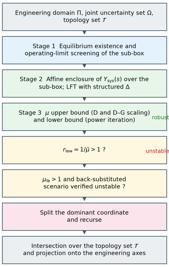
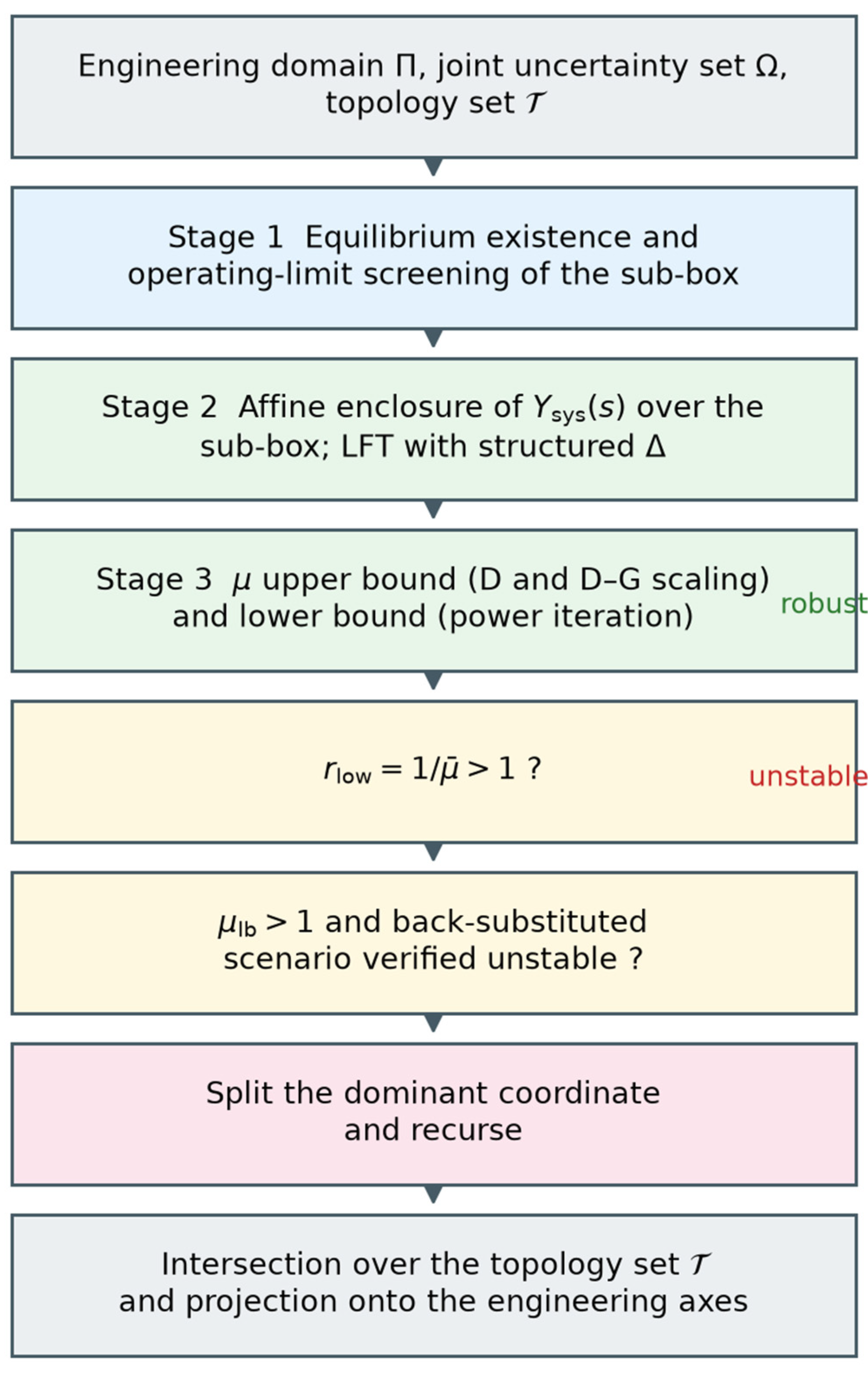
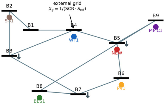
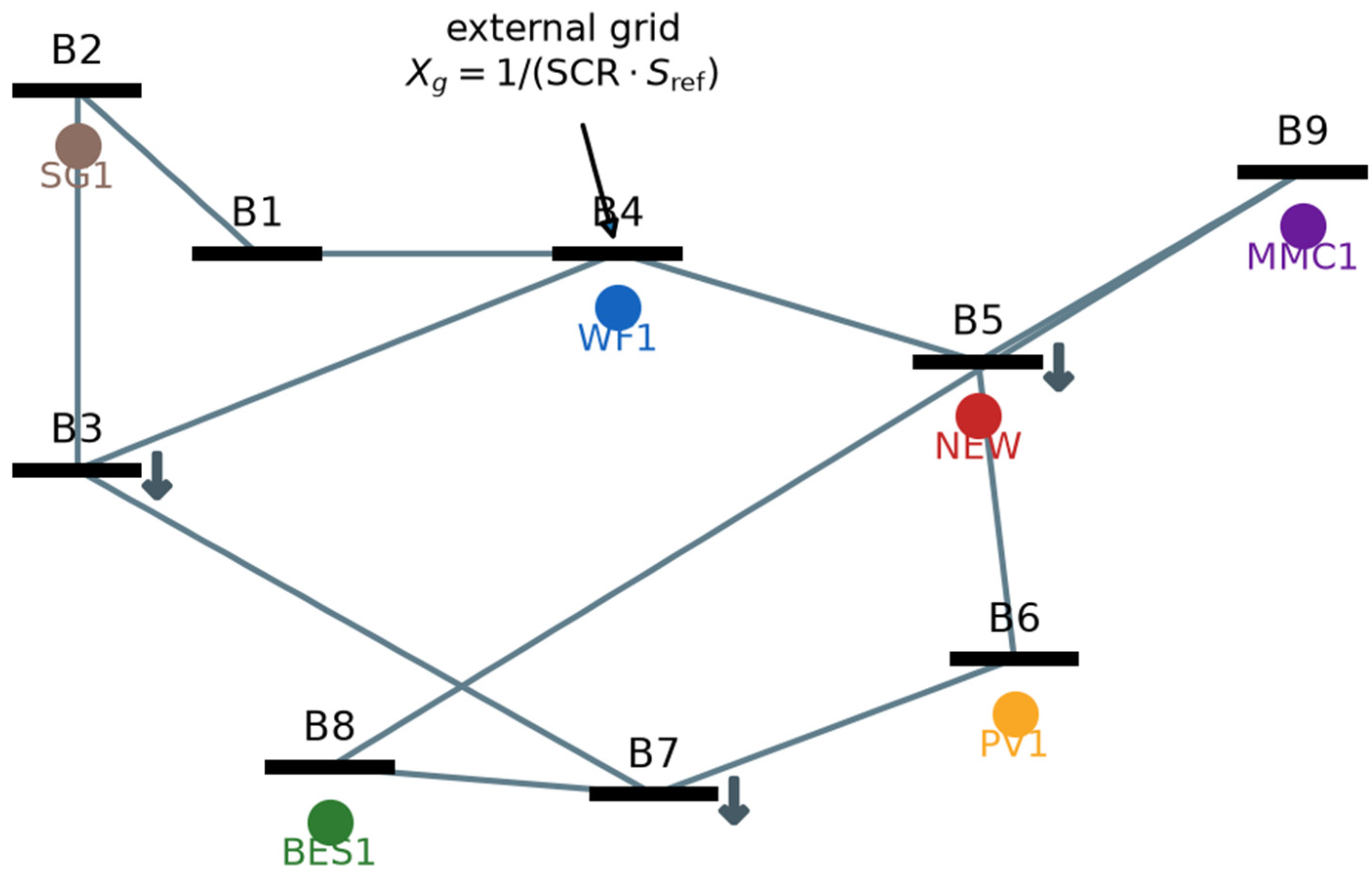
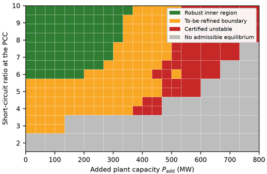
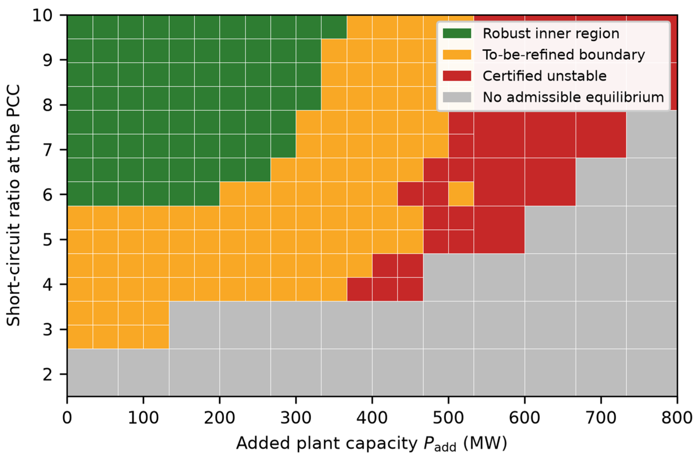
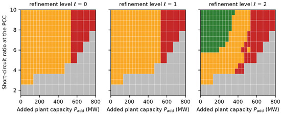
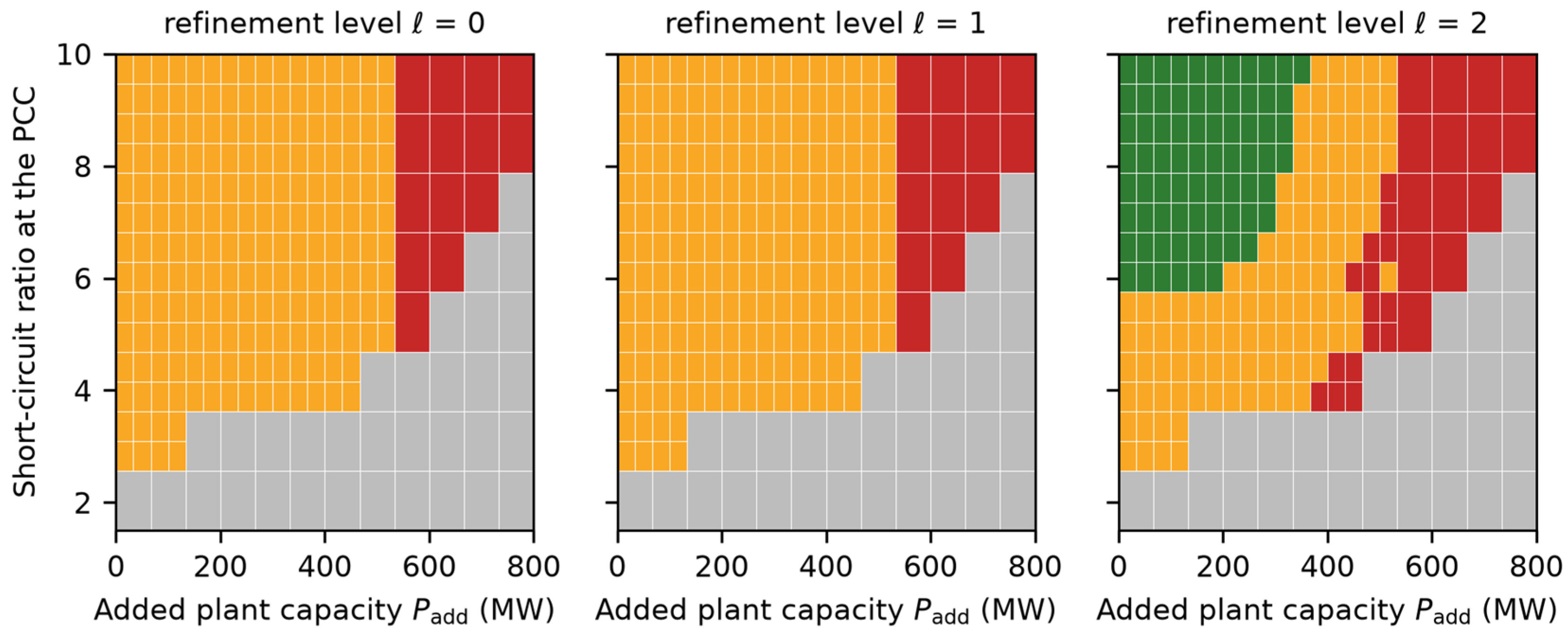
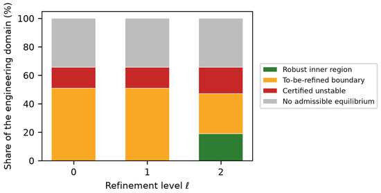
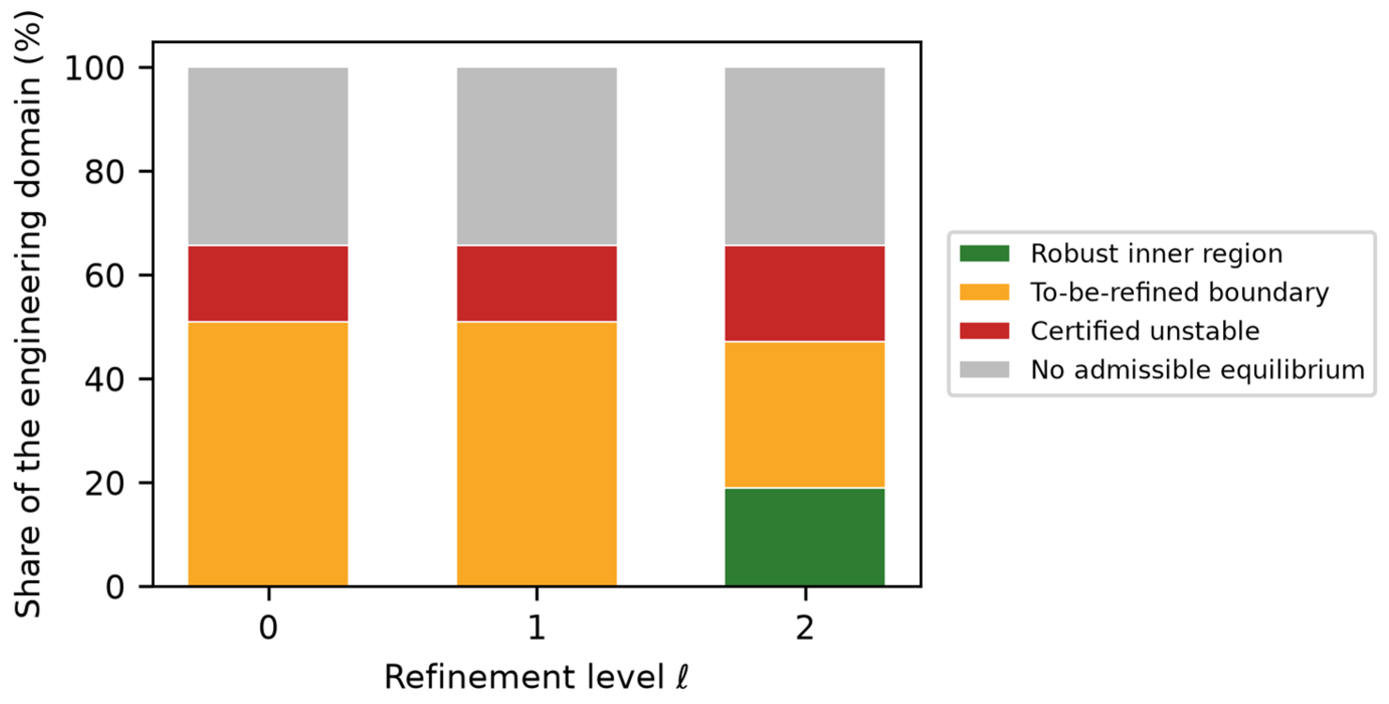
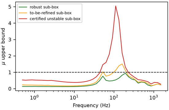
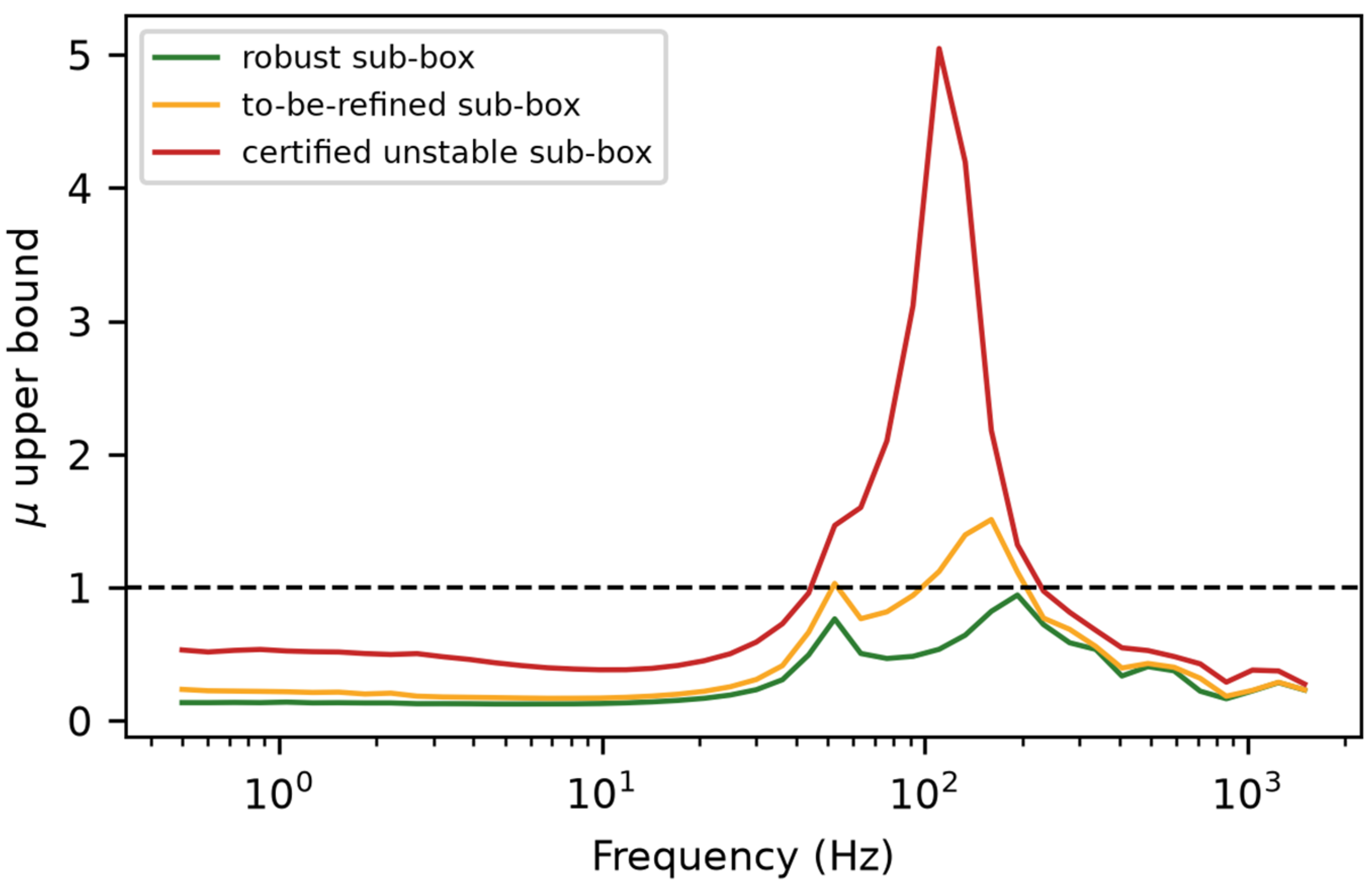
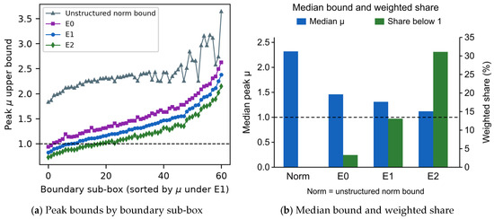
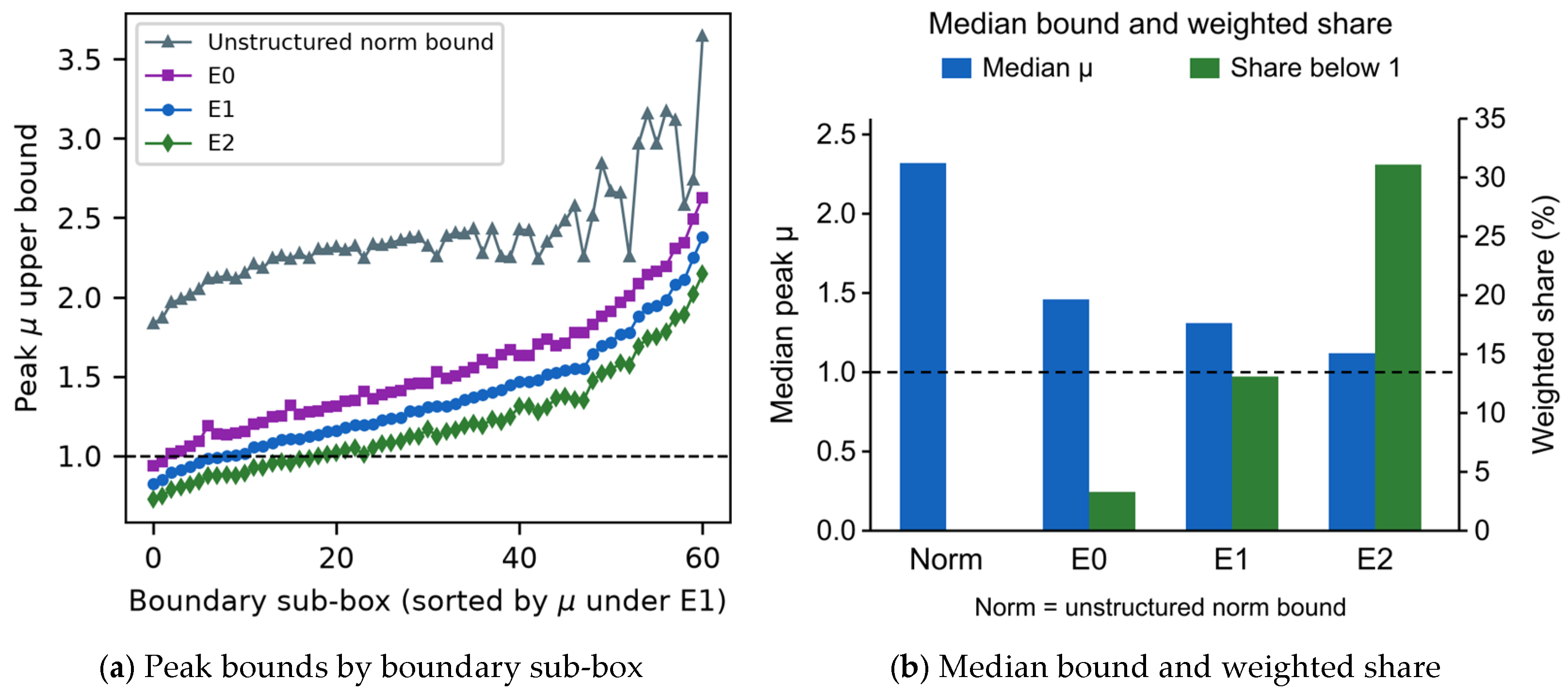
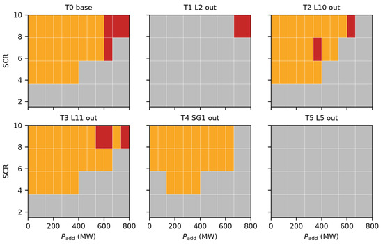
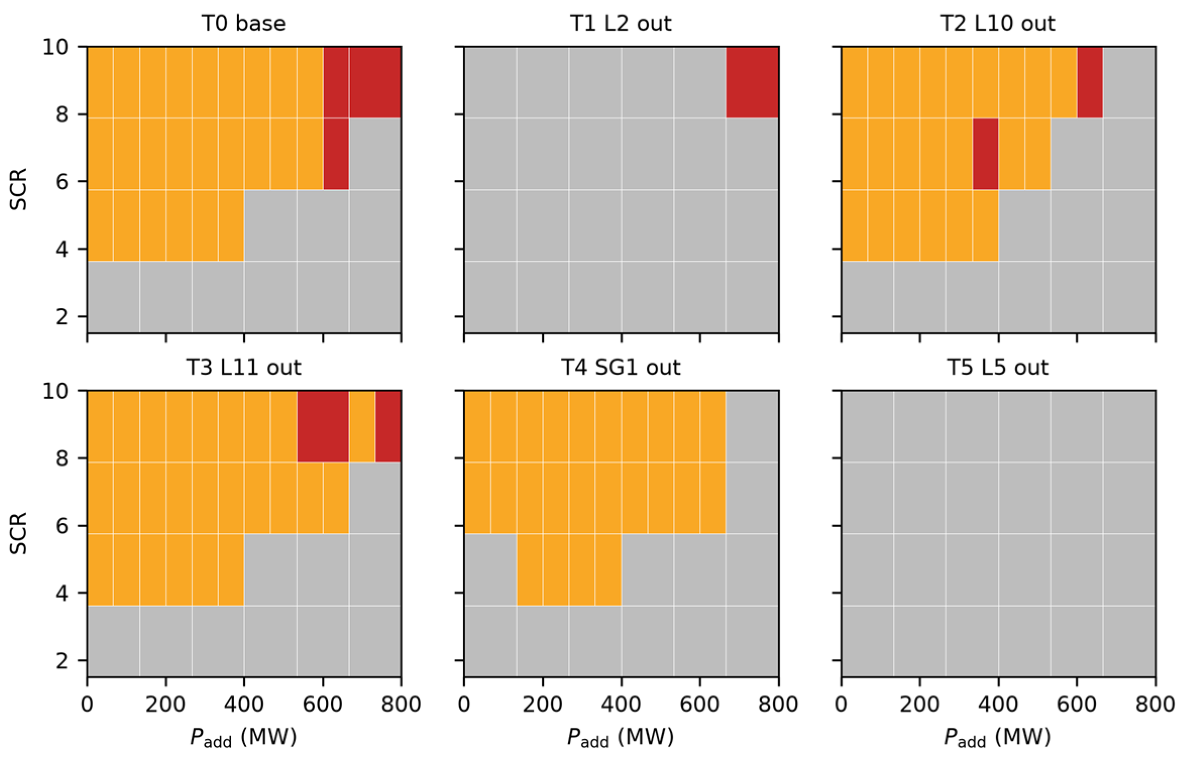
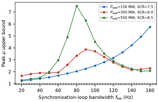
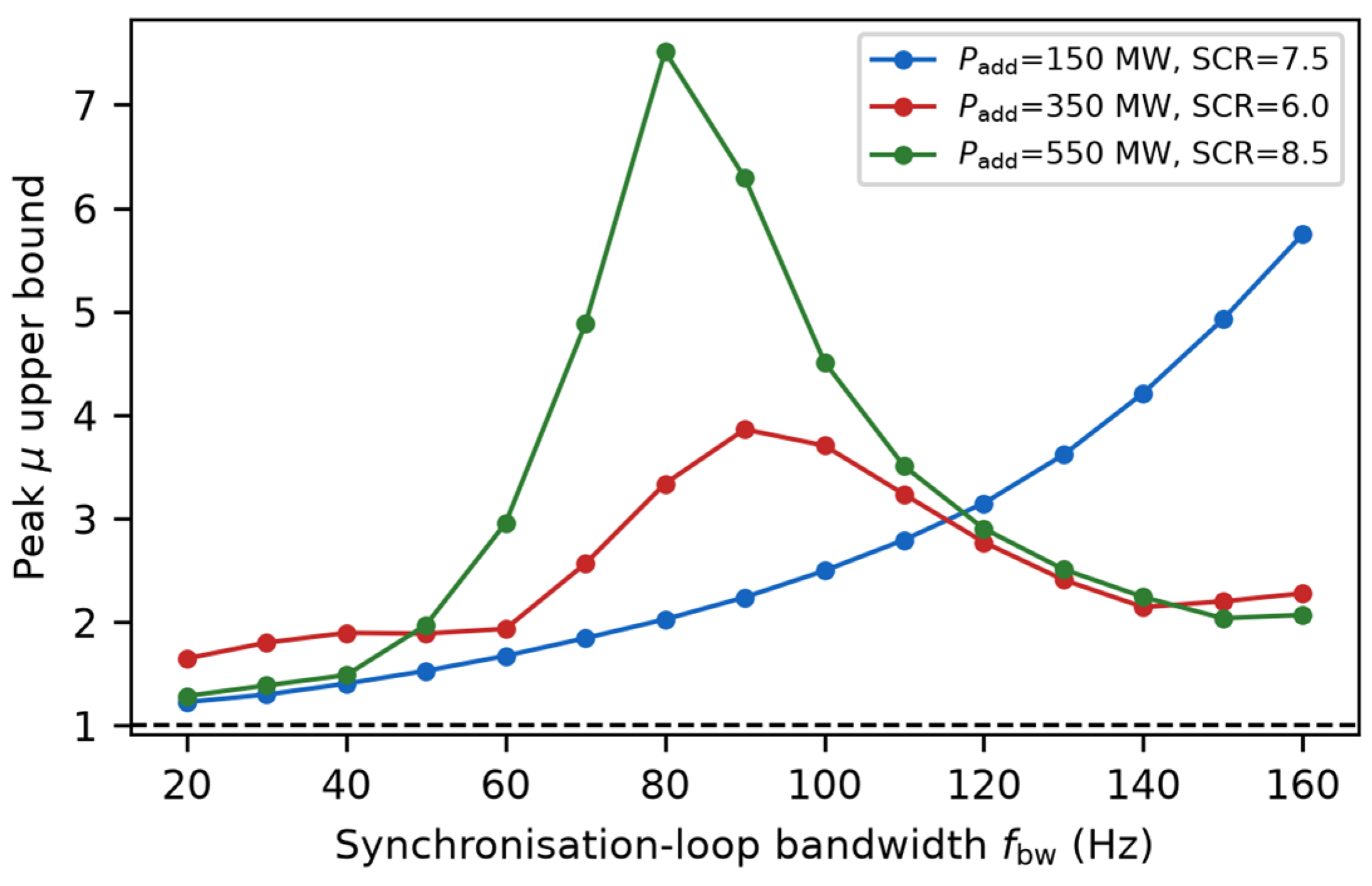
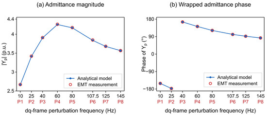
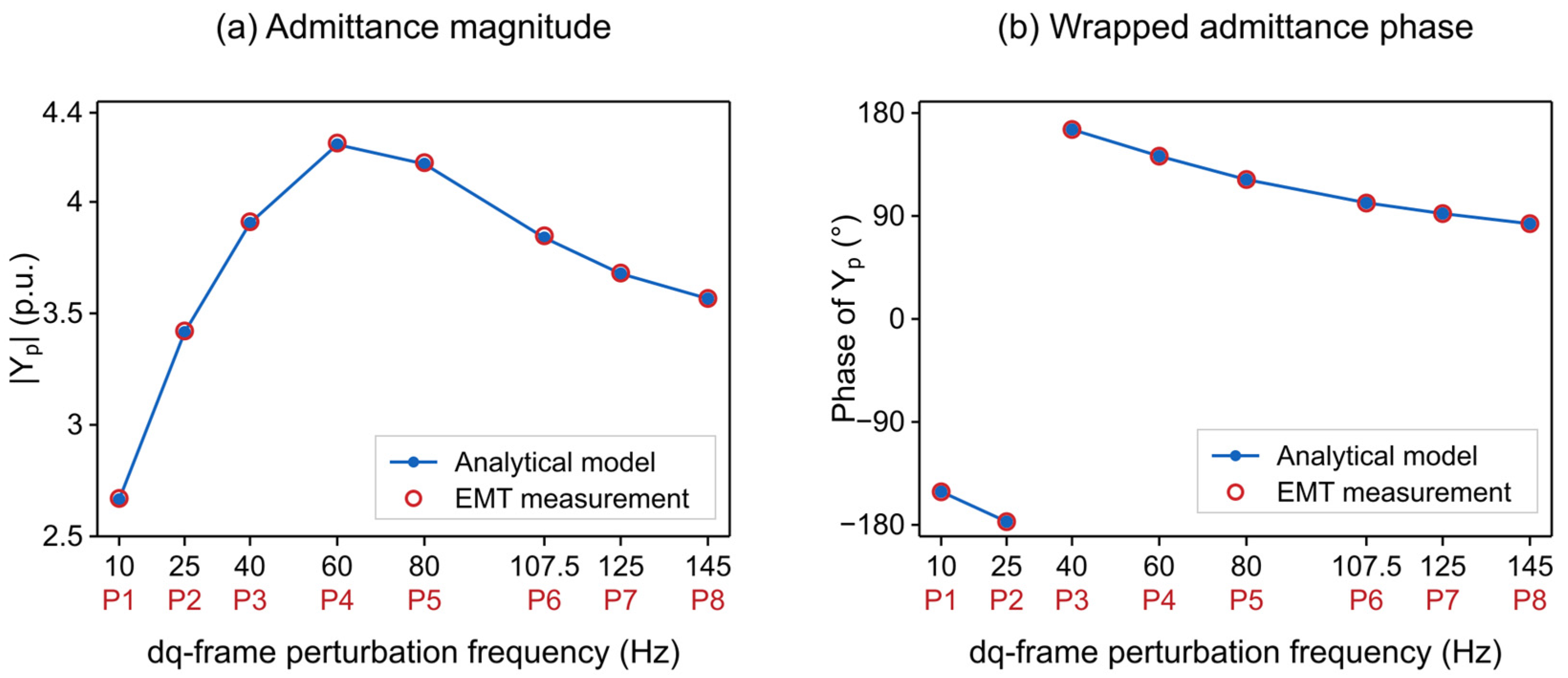
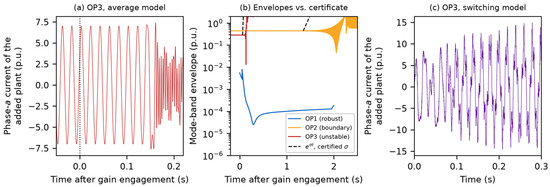
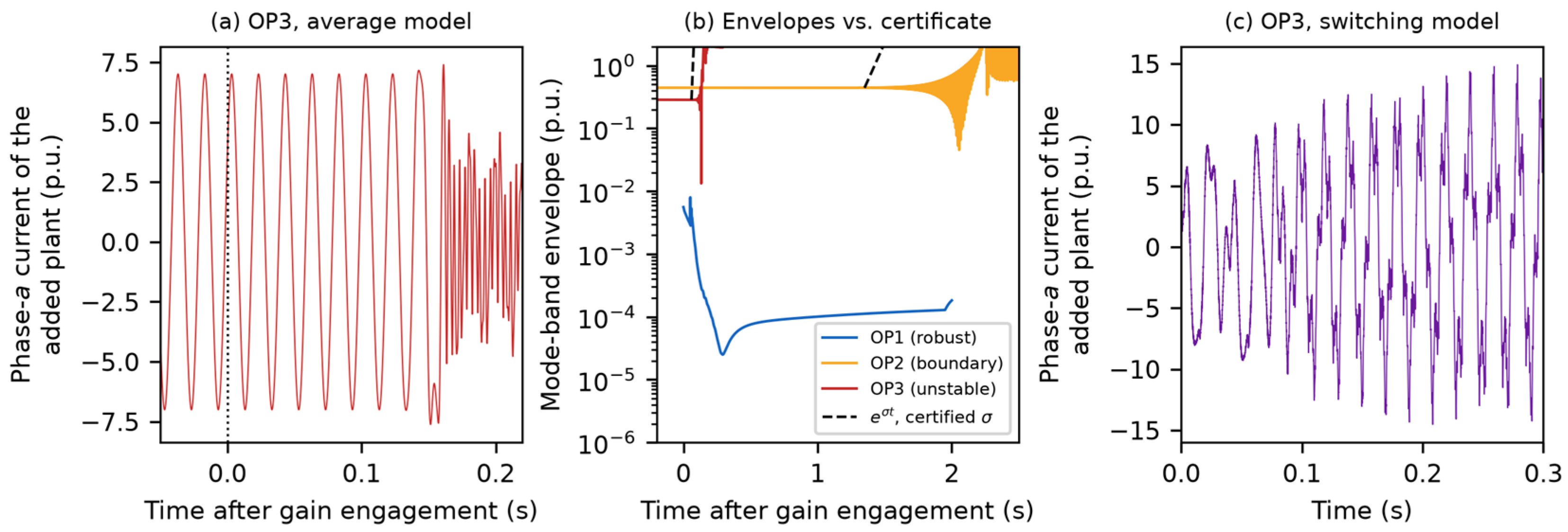

Disclaimer/Publisher’s Note: The statements, opinions and data contained in all publications are solely those of the individual author(s) and contributor(s) and not of MDPI and/or the editor(s). MDPI and/or the editor(s) disclaim responsibility for any injury to people or property resulting from any ideas, methods, instructions or products referred to in the content. |
© 2026 by the authors. Licensee MDPI, Basel, Switzerland. This article is an open access article distributed under the terms and conditions of the Creative Commons Attribution (CC BY) license.