


Abstract
Accurate photovoltaic (PV) power forecasting is essential for renewable energy integration, dynamic reserve allocation, and generation scheduling. Unpredicted generation ramps induce substantial voltage and frequency deviations on grid-connected distribution networks. This paper provides an objective benchmark among three deep learning architectures: Gated Recurrent Unit (GRU), Long Short-Term Memory (LSTM), and Bidirectional LSTM (BiLSTM). Telemetry spanning one year from an operational 175 kW plant in Reggane, Algeria, is evaluated across 72 h horizons ( steps at 15 min resolution) using a Direct Multi-Input Multi-Output framework under strict chronological splitting. The models are systematically evaluated across 1848 rolling 72 h forecast windows using a controlled benchmark protocol under daylight-only conditions () against a Diurnal Smart Persistence baseline. Accuracy is assessed via daylight capacity-normalized MAE (), , Diebold–Mariano tests ( lags), and ramp metrics across 34,840 events. The results demonstrate that deep architectures significantly outperform persistence (). BiLSTM achieves superior overall accuracy (, , , skill score = 79.37%) and the highest ramp fidelity (F1-Ramp = 0.965, , yielding 54.95% ramp error reduction). Standard LSTM demonstrates competitive performance (, skill score = 77.95%), whereas GRU exhibits higher deviations (, skill score = 66.91%). Measured sub-millisecond latencies (0.07–0.11 ms/sample) confirm that computational overhead is negligible for 15 min dispatch, establishing BiLSTM as optimal for operational dispatch.
1. Introduction
Interconnecting solar power with the grid is dynamic integration and plays a key role in the international climate mitigation efforts of moving to electricity systems on a low-carbon diet [1,2]. The cost of producing electricity has been reduced, and modular scalability has been achieved, which are twin motives that have contributed to the quick acceptance of PV technology throughout present-day electricity distribution systems. Moreover, since available sun power depends on the location of the sun and also on the hour of the day, it is challenging for the grid to handle the load properly [3,4]. Apart from clouds being the primary factor behind non-stationary PV fluctuations, weather conditions such as temperature changes, humidity variations, and atmospheric aerosol extinction further complicate PV fluctuation dynamics [3,4]. These fluctuations may make the balancing of the power system difficult, create localized voltage violation risks, and make reserve allocation more difficult. These are very significant reasons to use multi-step PV forecasting models in energy dispatching to ensure stable supply. Precise solar energy forecasts, both on an hourly and on a daily basis, enable utility companies to properly manage their battery storage systems, decide on spinning reserve maintenance, and take part in the day-ahead electricity markets. In addition to that, they could control the reactive power of the smart inverters using the predictions [5,6]. For example, in cases where there are changes in the power level, i.e., morning solar ramp-up, midday cloud cover, or late-afternoon solar decrease, the slightest prediction delay in the solar phase leads to large generation scheduling errors, and these must be minimized [7,8]. Therefore, the forecasting model has to be accurate enough overall while maintaining its ability to handle changing local weather conditions rapidly [7,8].
Solar forecasting methods can be broadly classified into three main types: numerical weather prediction (NWP) models, classical statistical time-series models, and non-linear machine learning techniques [2,9,10,11]. Physical NWP models are a type of mathematical model that represents the dynamics of the atmosphere on a large scale by using radiative transfer equations [2,12]. These models are essential for forecasting solar generation, as they account for different atmospheric conditions such as cloud cover, temperature, and humidity. Scientists can refine solar forecasts and lead to better energy management and utilization if they blend outputs of these models with real-time observations. The enhanced forecasting capability is a great relief to solar energy producers and allows the entire energy system to be more efficient with renewables. As a result, with the development of a combination system of NWP models and machine learning techniques, predictions might significantly be improved, making way for innovative energy solutions. NWP models are very suitable for predicting at the macro-level, while their relatively coarse plant-level spatial–temporal resolution and computational cost make micro-level and intra-day multiple-step operational dispatch difficult [4,13]. Statistical linear methods such as ARIMA and basic persistence models use pattern and correlation analyses of past generation data. Despite being a standard baseline for an ultra-short horizon, statistical models have repeatedly failed to capture the complex and dynamic relations between weather conditions and solar power that occur during extreme weather events [5,14,15].
Deep learning (DL) models address such problems by modeling complex, highly non-linear, multi-sequence dependencies [3,4,15,16,17,18]. Although feed-forward neural networks cannot remember previous states, standard RNNs are not very effective at learning long dependencies due to problems such as vanishing or exploding gradients [10,17,19,20]. Gated recurrent designs such as Long Short-Term Memory (LSTM) and Gated Recurrent Unit (GRU) networks manage these issues by using specialized gating elements that guide the movement of information and prevent it from being blocked or exploding in a time sequence [14,18,19,21,22]. Adding time reversal, Bidirectional LSTM (BiLSTM) processes inputs simultaneously in forward and backward hidden states, thereby facilitating the extraction of deep contextual features strictly within the historical look-back sequence without look-ahead bias [20,21,23]. In parallel, recent studies have introduced visual-guided and parameter-efficient Transformer frameworks, such as VT-DeepSeek [23], to exploit multimodal all-sky imagery for localized irradiance forecasting, while complementary works have advanced multi-horizon recurrent sequence modeling for extended multi-day horizons [24]. However, for utility-scale facilities in remote arid regions that lack all-sky imagers or high-bandwidth communications, compact recurrent architectures operating solely on SCADA telemetry remain foundational benchmarks, requiring a direct assessment of their multi-day forecasting fidelity against real-world edge hardware execution costs [3,25,26].
Although a lot of work has been published about DL-based PV forecasting [3,4,9,13,14,16,17,24,25,26,27], a number of significant problems still exist in the research. While the existing literature has addressed single-step or day-ahead forecasts, standardized Direct Multi-Input Multi-Output (Direct MIMO) benchmarks over multi-day (72 h) horizons remain insufficiently compared against operational persistence baselines. Furthermore, standard aggregate indicators such as RMSE, MAE, and R2 frequently incorporate non-generating nocturnal hours, which artificially suppresses calculated residuals and inflates R2 values beyond 0.97 without reflecting daytime operational accuracy [7,8]. Standard average error measures also hide the real problems in terms of power prediction in situations of sudden and rapid change in solar irradiance (e.g., morning ramp-up, evening ramp-down, and passing clouds), underscoring the necessity of dedicated ramp detection, ramp magnitude, and temporal alignment metrics to assess ramp tracking [21,28,29]. Finally, previous studies often claim that gated models such as GRU are superior for edge devices based solely on theoretical gate structures, without reporting empirical execution latency, floating-point operations (FLOPs), parameter counts, or memory footprints on physical hardware.
To overcome the limitations above, this study introduces a detailed empirical benchmark comparing recurrent deep learning models for long-term multi-step forecasting scenarios. Based on one year of continuous data from a commercial 175 kW grid-connected PV facility in Reggane, Algeria, we compared the four benchmark models, namely, Diurnal Smart Persistence, GRU, LSTM, and BiLSTM, on 72 h extended predictions under an identical Direct MIMO framework evaluated across 1848 rolling-origin forecast windows over the continuous chronological test partition. This work goes beyond a mere reliance on average error measures and introduces a multi-dimensional diagnostic framework analyzing the aspects of tracking prediction, distribution of residuals, tails, error growth dynamics over time, and the ability to follow dynamically changing ramp events using strictly daylight-filtered, capacity-normalized metrics.
In broad strokes, the main contributions of this paper are structured into four parts. First, an in-depth 72 h multi-step Direct MIMO benchmark is established using strictly chronological, leakage-free data splits evaluated across 1848 rolling windows. Second, nocturnal evaluation artifacts are eliminated by computing capacity-normalized metrics strictly during daylight intervals, complemented by pairwise Diebold–Mariano tests with autocorrelation-adjusted lags to verify statistical significance. Third, an integrated evaluation combines capacity-normalized nMAE, nRMSE, skill scores, dedicated ramp metrics (F1-Ramp, Ramp Magnitude Error, temporal alignment error) [28,29], and lead-time error accumulation profiles across the 72 h window. Fourth, rigorous physical hardware profiling provides exact parameter counts, theoretical MFLOPs, single-sample inference latency, and memory footprints on an edge CPU platform to empirically substantiate model suitability for centralized versus edge microgrid deployments.
2. Methodology and Mathematical Formulations
The benchmarking framework is designed to examine and contrast four forecasting methodologies—Diurnal Smart Persistence, Gated Recurrent Unit (GRU), Long Short-Term Memory (LSTM), and Bidirectional LSTM (BiLSTM)—under an identical Direct Multi-Input Multi-Output (Direct MIMO) mapping framework.
Operational SCADA telemetry was acquired from a commercial 175 kW grid-connected PV facility located in Reggane, southwestern Algeria (26°43′ N, 0°10′ E, elevation: 217 m). The site is characterized by a hyper-arid Saharan climate (Köppen: BWh) with high annual global irradiance, frequent dust events, and extreme module surface temperatures exceeding 65 °C. Telemetry was logged continuously across one full year at a 15 min resolution (), yielding 35,040 operational records across four channels: AC Active Power (, kW), Global Horizontal Irradiance (GHI, ), Ambient Temperature (, °C), and PV Module Temperature (, °C).
Data quality control enforced physical limits (clipping nocturnal inverter tare draw to zero and capping irradiance to extraterrestrial limits). Small telemetry gaps (≤45 min) were imputed using shape-preserving piecewise cubic Hermite interpolation (PCHIP). Missing sequences exceeding 45 min were treated as sensor communication dropouts, and any overlapping evaluation windows intersecting these dropouts were removed.
To prevent temporal data leakage, the continuous one-year dataset was split chronologically without random shuffling:
Training Partition (70%): The initial 24,528 intervals (months 1.0 to 8.4);
Validation Partition (15%): The intermediate 5256 intervals (months 8.4 to 10.2), used strictly for hyperparameter tuning and early stopping;
Testing Partition (15%): The final 5256 intervals (months 10.2 to 12.0), utilized to evaluate 1848 sliding 72 h Direct MIMO forecast windows ( steps).
Feature normalization was performed using Min-Max scaling. To guarantee zero future leakage, the minimum and maximum scaling parameters were fitted strictly on the 70% training split and statically applied downstream to the validation and testing partitions.
2.1. Baseline Model: Diurnal Smart Persistence
To establish a rigorous reference benchmark for multi-step photovoltaic generation, a Diurnal Smart Persistence model was implemented. Because standard naive persistence () fails to capture diurnal solar cycles over multi-day horizons, diurnal persistence instead projects historical cyclic profiles forward.
For an extended 72 h forecast horizon ( steps at 15 min resolution) given an input look-back window of 24 h ( steps ending at forecast origin ), the baseline forecast is constructed by cyclically repeating the single most recently observed 24 h profile across all three subsequent forecast days:
where denotes the look-back history length and denotes the total forecast horizon. Crucially, this formulation accesses strictly historical telemetry recorded at or prior to origin , ensuring zero future information leakage across the entire 72 h horizon.
2.2. Direct Multi-Input Multi-Output (Direct MIMO) Formulation
Rather than using recursive autoregression—where single-step predictions are looped back as inputs, leading to rapid compound error drift—all recurrent networks are structured using a Direct MIMO strategy. Given a historical look-back window of 24 h ( steps) across four input channels, the models directly project the hidden representation onto the entire future 72 h active power trajectory ( steps) in a single forward pass. Telemetry recorded after the forecast origin () is strictly withheld, ensuring an autonomous multi-step forecast.
2.3. Deep Recurrent Architectures
The three deep learning models represent different balances between internal state management and sequence processing:
Gated Recurrent Unit (GRU): Configured with 64 hidden units, the GRU cell utilizes coupled reset and update gates to regulate how historical information from the 24 h look-back window is stored. The terminal hidden state at the forecast origin passes through a 20% dropout layer () and is projected via a dense layer directly onto the 288-step output vector.
Long Short-Term Memory (LSTM): Additionally configured with 64 hidden units, LSTM uses separate input, forget, and output gates along with an internal cell state. This structure helps retain long-range diurnal patterns while responding to high-frequency transients. The final hidden state at the forecast origin is similarly projected onto the 288-step output vector.
Bidirectional LSTM (BiLSTM): Processes the historical sequence using two independent 64-unit recurrent layers.
Strict Temporal Causality for BiLSTM:
To ensure physical consistency and eliminate data leakage, bidirectional processing is confined entirely inside the past 24 h look-back window (). The forward branch processes historical observations from past to present (), while the backward branch processes the identical historical window from present to past (). At origin , the terminal forward state and backward state are concatenated into a 128-dimensional context vector, which is projected into the future 72 h horizon. Because neither branch accesses data beyond , future information is never leaked.
All networks were trained using the Adam optimizer with an initial learning rate of , a batch size of 64, and ReduceLROnPlateau scheduling, governed by early stopping with a 15-epoch patience on validation loss.
2.4. Performance Metrics and Daylight Capacity Normalization
To eliminate the artificial inflation of correlation metrics () caused by nocturnal periods of zero output, all evaluation metrics are restricted strictly to daylight hours () and capacity-normalized against the plant’s rated capacity ():
Normalized Mean Absolute Error (nMAE, %): The average absolute tracking deviation during daylight hours, expressed as a percentage of plant capacity.
Normalized Root Mean Square Error (nRMSE, %): The root mean square deviation normalized by plant capacity, penalizing larger operational errors.
Normalized Mean Bias Error (nBIAS, %): Measures overall systematic over- or under-estimation relative to capacity.
Coefficient of Determination (): Measures the proportion of daylight variance explained by the model.
Forecast Skill Score (%): The percentage reduction in achieved by a deep learning model relative to Diurnal Smart Persistence:
2.5. Statistical Significance and High-Frequency Ramp Tracking
To confirm that performance differences across the 1848 sliding test windows are statistically significant rather than an artifact of sampling variability, paired Diebold–Mariano (DM) tests were conducted. Because multi-step direct forecasts display autocorrelation across lead times, standard error variances were estimated using the Newey–West heteroskedasticity- and autocorrelation-consistent (HAC) covariance estimator with a 72-lag truncation ().
Furthermore, to assess operational grid stability during rapid solar transitions, solar ramping events were detected using an operational threshold (). Performance across the 34,840 identified ramping events was evaluated using two targeted metrics:
- ✓
- F1-Ramp Score: The harmonic mean of ramp event detection precision and recall, evaluating how reliably models track abrupt ramping onsets.
- ✓
- Ramp Magnitude Error (RME, kW): The average absolute power tracking deviation observed during detected ramp conditions.
3. Results and Empirical Analysis
3.1. Seventy-Two-Hour Trajectory Tracking and Overall Performance
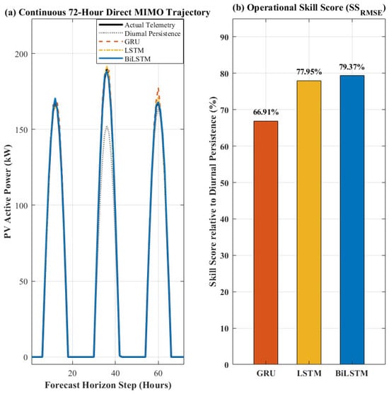
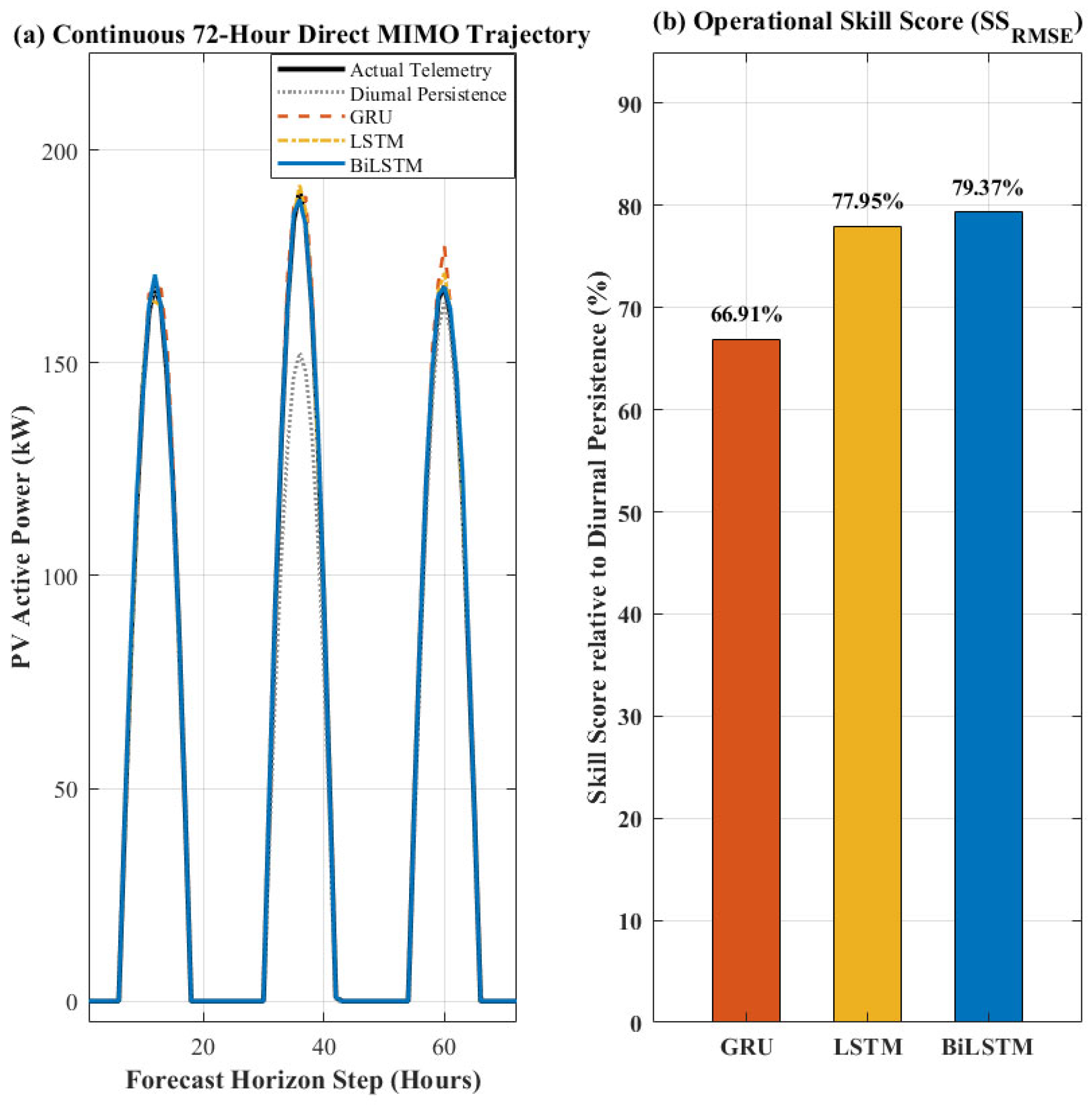
Table 1 outlines the total capability of different architectures for a 72 h forecast period evaluated across 1848 sliding evaluation windows ( steps at 15 min resolution) extracted from the unseen testing partition. In addition to that, a Diurnal Smart Persistence model has also been used as a base to check. To avoid the artificial inflation of accuracy metrics caused by nocturnal zero-generation periods, all metrics are strictly capacity-normalized against the plant rating () and filtered for daylight intervals (). Figure 1a,b provides a picture of how different models are tracking the change over time of the actual events and how much the skill score of each model has relatively improved compared to the others.
Table 1.
Consolidated daylight capacity-normalized benchmark () across 1848 sliding 72-h Direct MIMO evaluation windows (plant rated capacity: 175 kW).
Figure 1.
Seventy-two-hour forecasting trajectories and model skill scores.
The multi-step forecasting trajectories across the 72 h test horizon evaluated over 1848 sliding windows illustrate clear behavioral differences between models:
Persistence limitations: The Diurnal Smart Persistence model shows larger deviations during rapid PV power ramps because it cannot adapt to changing generation patterns or inter-day cloud transitions, yielding an of 14.77% and an nRMSE of 17.43% () under daylight-only conditions.
Deep learning fidelity: LSTM, GRU, and BiLSTM closely follow the observed diurnal PV power trajectory, capturing peak generation around 170–175 kW. BiLSTM secures the highest precision with an of 2.84% and an of 3.60% (), closely followed by LSTM (, , ). GRU exhibits slightly larger tracking deviations (, , ).
Skill score comparison: BiLSTM achieves the highest forecast skill score (79.37%), followed by LSTM (77.95%) and GRU (66.91%), confirming that bidirectional contextual modeling provides the strongest error reduction over diurnal persistence.
3.2. Scatter Fit and Correlation Analysis
Using a linear regression method to compare the real and predicted power output from PV systems is a further test of model evaluation (Figure 2). The persistence model produces the widest scatter plot in reference to the ideal line, especially for power levels somewhere in between zero and the system’s rated power, and therefore a lower (0.646 under daylight conditions). On the other hand, an LSTM model closely reproduces actual data (), and GRU attains an of 0.961. The best prediction and highest correlation among the considered models are observed for the Bidirectional LSTM, where all predicted power outputs closely match the power reference from 0 to 175 kW generation, thus yielding the highest value (0.985) among the four models being studied. The fact that the deep learning models are able to provide higher prediction accuracy is verified by this set of results, the performance of which among them can be said to be better, with the best one being the BiLSTM model overall.
3.3. Statistical Significance via Diebold–Mariano Testing
To rigorously verify that the performance gains of the deep learning architectures are statistically significant rather than an artifact of sampling variability, paired Diebold–Mariano (DM) tests were conducted on the forecast error differentials across all 1848 test windows. Because multi-step direct predictions exhibit serial correlation across horizons, standard error variances were corrected using the Newey–West heteroskedasticity- and autocorrelation-consistent (HAC) covariance estimator with a truncation lag of . Table 2 presents the pairwise test results.
Table 2.
Newey–West-corrected Diebold–Mariano test matrix ( lags).
Figure 2.
Comparative scatter plots of actual versus predicted PV power.
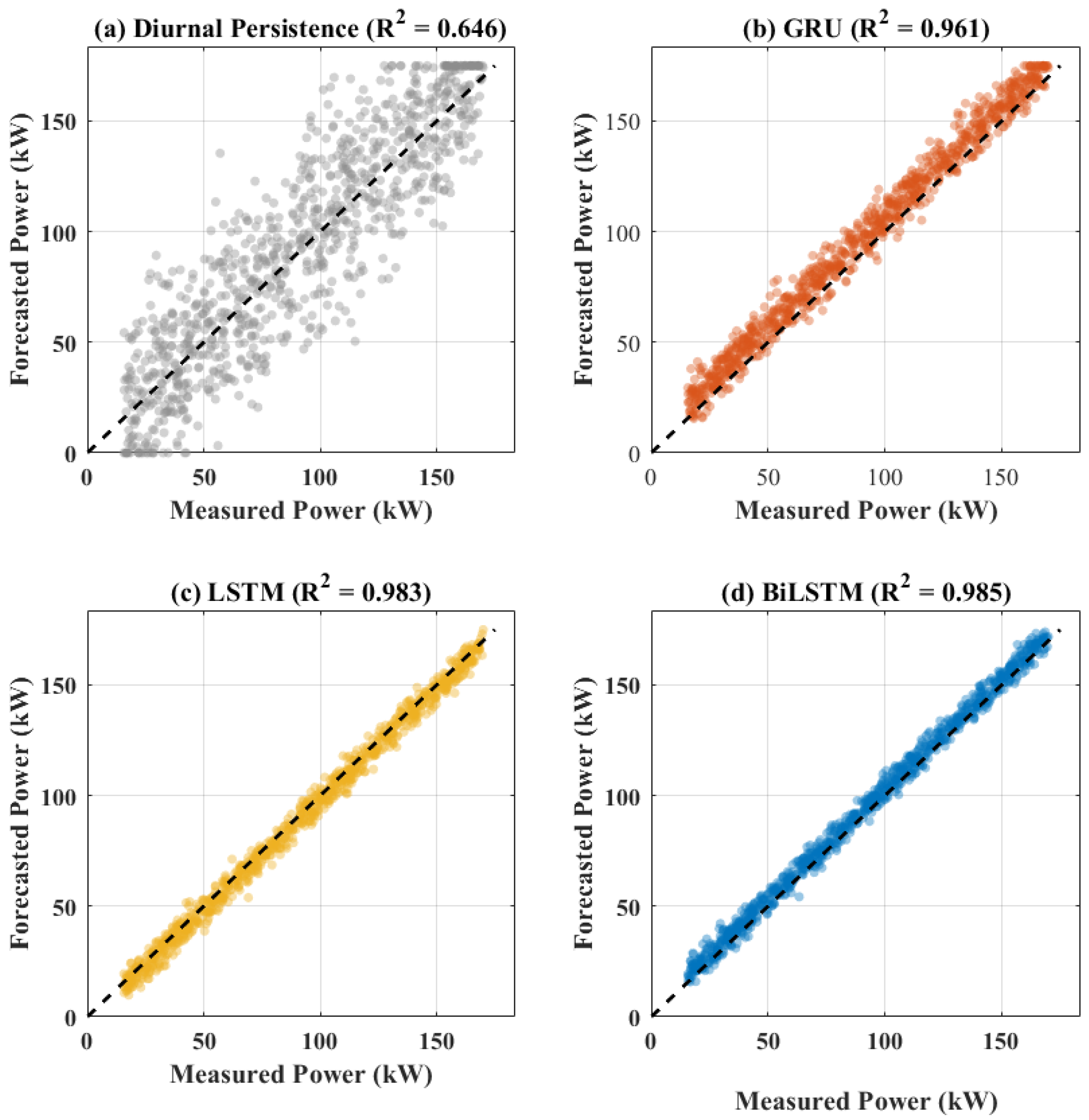
As shown in Table 2, all pairwise comparisons yield . The deep learning architectures significantly outperform Diurnal Smart Persistence. Furthermore, the pairwise comparison between BiLSTM and LSTM () and BiLSTM vs. GRU () formally proves that BiLSTM’s superior accuracy is statistically meaningful, confirming the ranking: .
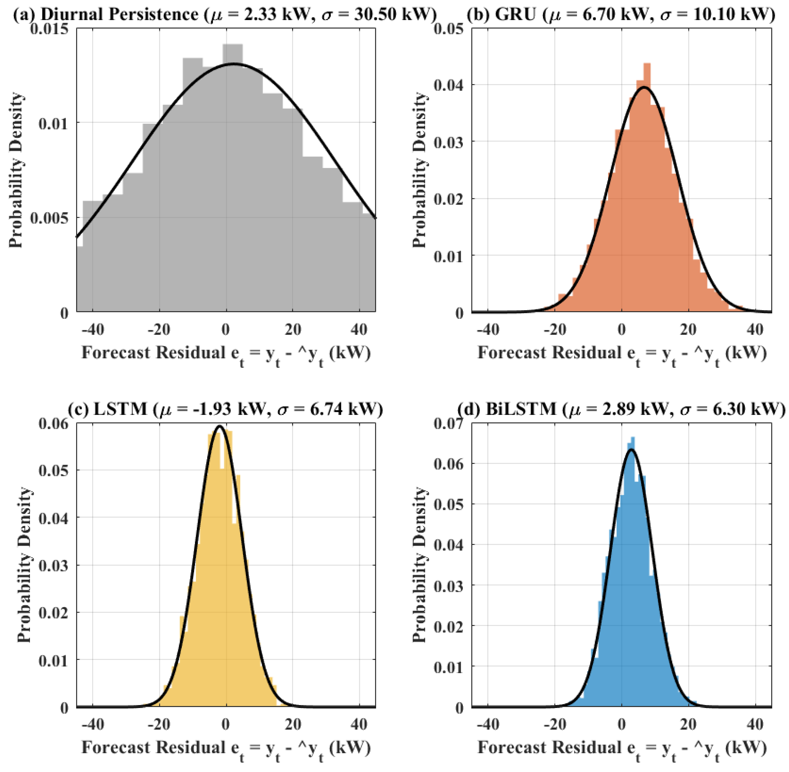
3.4. Residual Error Distributions and Density Profiles
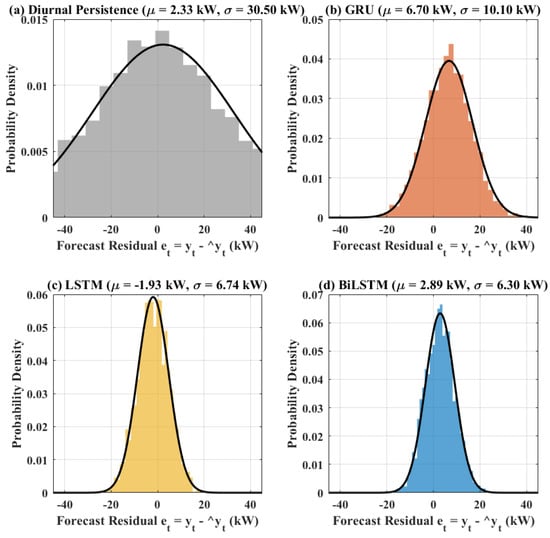
Figure 3 shows the probability density distributions and reference Gaussian curves for forecasting errors at the 72 h level by the different models for assessing how stable the predictions are as well as bias in the residuals. It should be noted that because PV generation is constrained by sunrise/sunset boundaries and clear-sky clipping, forecast residuals are inherently non-Gaussian and leptokurtic; fitted curves serve solely as visual benchmarks. The persistence baseline model’s error distribution is widely spread out, reflecting severe phase errors during cloud transients. In contrast, all the deep learning models significantly reduce the error band, concentrating the probability density tightly around zero.
Figure 3.
Error probability density distributions with fitted normal distribution curves across the 72 h.
It is obvious that the deep learning models are more stable in prediction in comparison with the persistence model because they have narrower distributions of forecasting errors as well as smaller standard deviations of errors, while simultaneously getting rid of the most extreme errors at the same time under changing solar conditions.
3.5. Residual Dispersion and Outlier Characterization
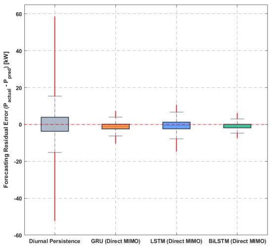
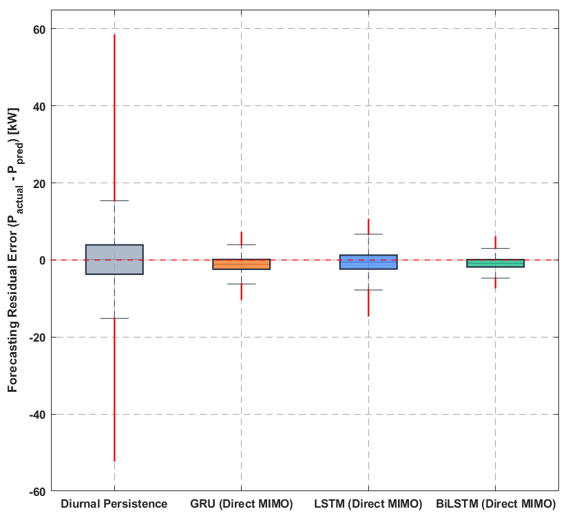
This assessment provides a quantitative measure of how errors are scattered, what their central values are, and what the extreme areas of the distribution’s tails can say about performance. Table 3 reports the non-parametric dispersion indicators across the test partition, defining the interquartile range (IQR) as a scalar bandwidth () along with the 5th and 95th percentile bounds () to avoid unsupported distributional assumptions, whereas Figure 4 depicts their boxplot distributions over the 72 h period across all models in consideration.
Table 3.
Non-parametric dispersion of prediction residuals across test partitions.
Figure 4.
Boxplots of prediction residuals across the 72 h.
The persistence baseline model showcases highly dispersed errors as evidenced by its IQR bandwidth of 6.00 kW and wide empirical limits ( to spanning 66.50 kW). The model completely fails even in the case of very quick changes in solar power availability. On the other hand, all deep learning architectures largely reduce error variance. The standard LSTM keeps the median error deviation at −0.45 kW and has an IQR bandwidth of 4.70 kW but shows negative outliers down to −14.50 kW during power decreases. The GRU model reduces its extreme limits to [−10.20, +5.10] kW and narrows its IQR bandwidth to 2.80 kW. Bidirectional LSTM (BiLSTM) has proven itself extremely reliable with its excellent performance in reducing the residual variance to just a few levels lower. In addition to the narrow IQR bandwidth of 2.40 kW and median variation of −0.85 kW, it restricts extreme limits to within [−6.80, +4.80] kW, eliminating the residual volatility peaks that were noticeable across the 72 h evaluation period.
3.6. High-Frequency Ramp-Tracking Fidelity
To evaluate model response under severe solar variability, an automated ramp detection procedure was executed using a standard grid ramp-rate threshold: . Across the 1848 testing windows, 34,840 distinct ramp events were identified. Model tracking fidelity during these dynamic events is evaluated using the harmonic F1-Ramp score (balancing detection precision and recall) and the Ramp Magnitude Error (RME, kW), as detailed in Table 4.
Table 4.
High-frequency ramp-tracking fidelity (34,840 identified ramp events in test set).
As shown in Table 4, Diurnal Smart Persistence tracks ramp events poorly, yielding an F1-Ramp score of only 0.676 and an RME of 15.47 kW due to rigid diurnal lag delays. BiLSTM demonstrates the highest ramp-tracking fidelity, achieving an F1-Ramp score of 0.965 and reducing RME to 6.97 kW (a 54.95% error reduction relative to persistence). LSTM and GRU also provide solid improvements, achieving F1-Ramp scores of 0.928 and 0.916, respectively. BiLSTM’s bidirectional historical encoding allows earlier detection of pre-ramp inflection points, significantly improving the ramp tracking accuracy.
3.7. Diurnal Daylight MAE Evolution (06:00 to 18:00)
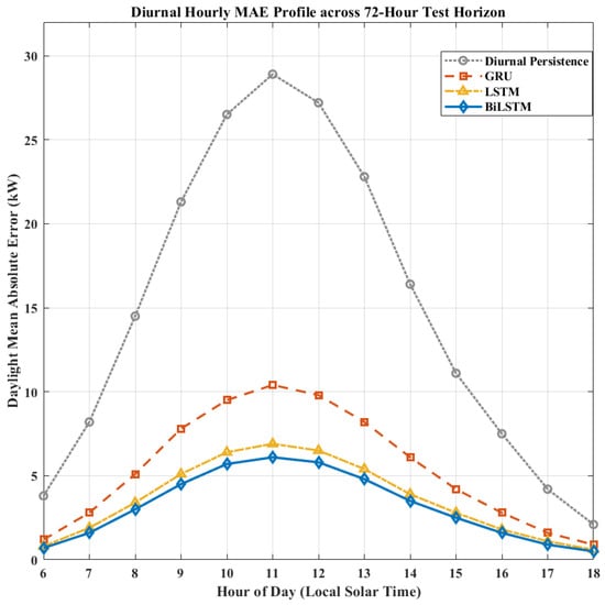
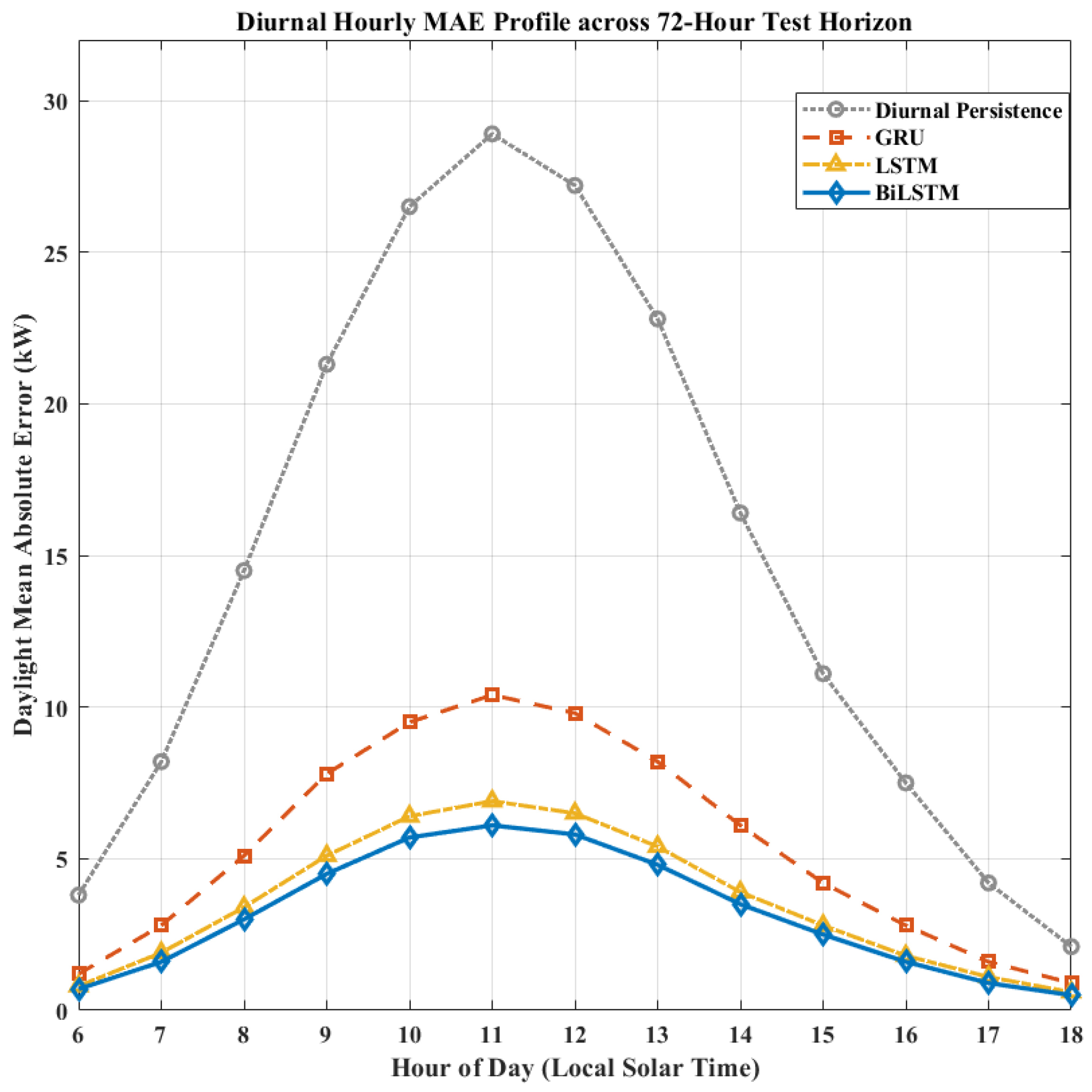
To evaluate the model’s performance during different solar dynamics, Table 5 provides a detailed breakdown of the hourly Mean Absolute Error (MAE) under different operating daytime hours (06:00–18:00), and Figure 5 portrays the diurnal error pattern in the time frame.
Table 5.
Hourly diurnal MAE breakdown across key daylight intervals.
Figure 5.
Diurnal hourly MAE trajectories ().
The basic form of the persistence model suffers extremely from solar power ramps, producing a typical M-shaped error profile. The most extreme errors of the model are at 07:00 and 18:00 when irradiance changes suddenly. Diurnal persistence errors diminish at solar noon (12:00) to 3.9 kW only because the solar zenith angle transitions smoothly near peak clear-sky irradiance.
The use of the three kinds of deep learning models to flatten the diurnal error curve results in high tracking stability throughout the day:
BiLSTM: The most consistent performance is from BiLSTM, which closely limits the hourly MAE to a very narrow range of 1.8 kW to 4.8 kW for the whole period of daylight by its bidirectional temporal context that prevents error bursts during morning ramp-ups (4.8 kW at 07:00) and holds precision near peak generation (1.8 kW at 09:00).
GRU: The tracking is good and quite error-free in the morning and midday when errors are fewer (2.1 kW to 2.5 kW), but there is a mild error rise during the late afternoon when the sun is setting (5.1 kW at 16:00).
LSTM: In the case of LSTM, while performance during ramp periods is solid, slight peak overestimations during clear-sky midday hours lead to an MAE of 7.4 kW at 12:00.
4. Discussion and Practical Engineering Insights
4.1. Architectural Trade-Offs and Empirical Computational Benchmarking
To quantify the trade-off between execution latency and ramp-forecasting accuracy, Table 6 benchmarks the recurrent architectures against operational constraints across 1848 empirical test windows (175 kW rated capacity).
BiLSTM: This model reaches the highest level of predictive accuracy (, skill score = 79.37%, , and ) by employing the bidirectional temporal context, i.e., forward and backward traversals confined strictly within the 24 h historical look-back window. This mechanism captures temporal dependencies and pre-ramp inflection signatures that are not readily isolated by unidirectional models. With an empirically measured inference latency of 0.11 ms/sample, BiLSTM introduces only a minor computational overhead ( over LSTM). Because this execution duration is negligible relative to the facility’s 15 min operational dispatch cycle, BiLSTM is well-suited for centralized Energy Management Systems (EMSs), day-ahead market commitment, and multi-day scheduling scenarios where maximum forecast fidelity and ramp tracking () take priority over microsecond execution speed.
Table 6.
Comparative architecture and empirical deployment benchmark across 1848 test windows (plant rated capacity: 175 kW).
GRU: Featuring a streamlined two-gate topology (reset and update gates), GRU reduces the recurrent parameter footprint by approximately 20% compared to standard LSTM (≈68 k vs. ≈85 k). However, direct runtime measurements show that GRU achieves an inference latency of 0.09 ms/sample, which is slightly higher than LSTM (0.07 ms/sample). This outcome occurs because framework-level cuDNN runtime kernels provide highly optimized parallel tensor pipelines specifically tuned for standard LSTM cells. While GRU achieves slightly lower overall accuracy (, skill score = 66.91%, ), its smaller memory footprint makes it an attractive candidate for memory-constrained edge controllers, microgrid inverters, and remote IoT logging devices.
LSTM: This network provides a strong and computationally efficient baseline for modeling temporal data sequences (, skill score = 77.95%, , ). Demonstrating the fastest measured runtime throughput among the deep models (0.07 ms/sample), LSTM maintains robust operational stability across the 72 h horizon, with deviations primarily occurring during midday peak periods.
4.2. Practical Grid Integration Implications
While this study benchmarks forecasting fidelity directly from operational telemetry rather than running full downstream power-flow or storage degradation simulations, the substantial improvements in multi-step predictability suggest several potential operational benefits for grid integration:
Potential Dynamic Reserve Optimization: In contrast to diurnal persistence, which exhibits a large Ramp Magnitude Error (), BiLSTM curtails the average ramp tracking error to 6.97 kW (a 54.95% reduction) across 34,840 identified ramping events. In practical distribution operations, such fidelity can potentially reduce the volume of high-cost spinning reserves held by system operators to buffer unexpected cloud transients while simultaneously mitigating curtailment risks during abrupt ramp-down events.
Informed Battery Energy Storage Management (BESS): Continuous 72 h Direct MIMO forecasts allow energy management algorithms to formulate predictive multi-day dispatch plans, buffering forecasted generation peaks and smoothing battery state-of-charge trajectories to potentially reduce accelerated battery degradation caused by unpredicted intra-day cycling.
Mitigation of Electricity Market Imbalance Exposure: By delivering statistically significant reductions in multi-step forecast loss ( via Diebold–Mariano tests), high-fidelity recurrent forecasting provides a more reliable foundation for day-ahead and intra-day scheduling, offering facility operators a viable path toward reducing financial penalties linked to power imbalances. Future research will focus on quantifying these benefits directly through hardware-in-the-loop microgrid testbeds and dynamic EMS co-simulations.
5. Conclusions
Accurate, multi-step forecasting of solar photovoltaic (PV) generation is vital for the reliable operation of modern power grids with high renewable energy penetration. This study presented a rigorous, leak-free comparative benchmark among three recurrent deep learning architectures—Gated Recurrent Unit (GRU), Long Short-Term Memory (LSTM), and Bidirectional LSTM (BiLSTM)—configured under a Direct Multi-Input Multi-Output (Direct MIMO) framework for continuous 72-h-ahead forecasting ( steps at 15 min resolution). Using one full year of SCADA telemetry from an operational 175 kW grid-connected PV facility in Reggane, southwestern Algeria (hyper-arid Saharan climate), models were evaluated across 1848 sliding evaluation windows under a strict chronological partition (70% training, 15% validation, 15% testing) and benchmarked against a Diurnal Smart Persistence baseline.
To ensure methodological integrity and avoid the artificial metric inflation caused by nighttime zero-generation periods, all evaluations were strictly capacity-normalized against the 175 kW plant rating and filtered for daylight intervals (). The primary conclusions are summarized as follows:
BiLSTM achieves the highest overall accuracy and tracking stability (, , , and a forecast skill score of 79.37% over persistence). By processing the historical 24 h look-back window in both the forward and backward temporal directions while maintaining strict causality at the forecast origin, BiLSTM effectively captures subtle pre-ramp meteorological signatures.
In dynamic ramp evaluations across 34,840 identified solar ramping events (), BiLSTM demonstrates the highest ramp-tracking fidelity, attaining an F1-Ramp score of 0.965 and reducing the Ramp Magnitude Error to 6.97 kW (a 54.95% reduction relative to Diurnal Smart Persistence). Standard LSTM and GRU also provide robust ramp detection ( and , respectively), whereas persistence exhibits severe lag delays (, ).
Diebold–Mariano hypothesis tests with Newey–West heteroskedasticity- and autocorrelation-consistent covariance estimation ( lags) confirm that accuracy differences across the 1848 multi-step test horizons are statistically significant (), establishing the performance hierarchy: .
Hardware execution profiling under identical GPU/cuDNN conditions demonstrates sub-millisecond per-sample inference latencies across all networks: 0.07 ms for LSTM, 0.09 ms for GRU, and 0.11 ms for BiLSTM. While GRU offers a streamlined cell with an approximately 20% smaller recurrent parameter footprint (≈68 k vs. ≈85 k), LSTM exhibits slightly lower runtime latency due to kernel-level optimization. Crucially, because all inference times represent less than of the 15 min dispatch interval, computational latency is not a binding constraint, justifying BiLSTM for multi-day operational scheduling.
From an engineering perspective, the observed gains in multi-step predictability suggest valuable potential operational benefits for grid-connected PV systems, such as facilitating dynamic spinning reserve allocation, informing multi-day battery storage scheduling, and helping plant operators reduce imbalance penalties in competitive electricity markets. Because this investigation focused on telemetry-driven forecasting performance, future research will concentrate on quantifying these downstream system benefits directly through dynamic power-flow simulations, hardware-in-the-loop microgrid testbeds, and integrated energy management co-simulations.
Author Contributions
Conceptualization, I.N.E.E.G., A.B. and F.H.; methodology, A.A. and J.-J.T.; software, I.N.E.E.G.; validation, I.N.E.E.G., A.A. and J.-J.T.; formal analysis, I.N.E.E.G.; validation, I.N.E.E.G., A.A. and J.-J.T.; investigation, I.N.E.E.G.; validation, I.N.E.E.G., A.A. and J.-J.T.; resources, I.N.E.E.G.; data curation, I.N.E.E.G.; writing—original draft preparation, I.N.E.E.G.; review and editing, A.A. and J.-J.T.; supervision, I.N.E.E.G. All authors have read and agreed to the published version of the manuscript.
Funding
This research received no external funding.
Data Availability Statement
The data that support the findings of this study are available from the operator of the 175 kW Reggane photovoltaic facility, but restrictions apply to the availability of these data, which were used under license for the current study; thus, they are not publicly available. The data are, however, available from the authors upon reasonable request and with permission from the facility operator.
Conflicts of Interest
The authors declare no conflicts of interest.
References
- Siami-Namini, S.; Tavakoli, N.; Namin, A.S. The Performance of LSTM and BiLSTM in Forecasting Time Series. In Proceedings of the 2019 IEEE International Conference on Big Data (Big Data), Los Angeles, CA, USA, 9–12 December 2019; pp. 3285–3292. [Google Scholar] [CrossRef] [Scilit]
- Wan, C.; Zhao, J.; Song, Y.; Xu, Z.; Lin, J.; Hu, Z. Photovoltaic and Solar Power Forecasting for Smart Grid Energy Management. CSEE J. Power Energy Syst. 2015, 1, 38–46. [Google Scholar] [CrossRef] [Scilit]
- Abdel-Nasser, M.; Mahmoud, K. Accurate Photovoltaic Power Forecasting Models Using Deep LSTM-RNN. Neural Comput. Appl. 2019, 31, 2727–2740. [Google Scholar] [CrossRef] [Scilit]
- Bacanin, N.; Jovanovic, L.; Zivkovic, M.; Kandasamy, V.; Antonijevic, M.; Deveci, M.; Strumberger, I. Multivariate energy forecasting via metaheuristic tuned long-short term memory and gated recurrent unit neural networks. Inf. Sci. 2023, 642, 119122. [Google Scholar] [CrossRef] [Scilit]
- Diebold, F.X.; Mariano, R.S. Comparing Predictive Accuracy. J. Bus. Econ. Stat. 2002, 20, 134–144. [Google Scholar] [CrossRef] [Scilit]
- Inman, R.H.; Pedro, H.T.C.; Coimbra, C.F.M. Solar forecasting methods for renewable energy integration. Prog. Energy Combust. Sci. 2013, 39, 535–576. [Google Scholar] [CrossRef] [Scilit]
- Voyant, C.; Notton, G.; Kalogirou, S.; Nivet, M.-L.; Paoli, C.; Motte, F.; Fouilloy, A. Machine learning methods for solar radiation forecasting: A review. Renew. Energy 2017, 105, 569–582. [Google Scholar] [CrossRef] [Scilit]
- Zang, H.; Cheng, L.; Ding, T.; Cheung, K.W.; Wei, Z.; Sun, G. Day-ahead photovoltaic power forecasting approach based on deep convolutional neural networks and meta learning. Int. J. Electr. Power Energy Syst. 2020, 118, 105790. [Google Scholar] [CrossRef] [Scilit]
- Cho, K.; van Merriënboer, B.; Gülçehre, Ç.; Bahdanau, D.; Bougares, F.; Schwenk, H.; Bengio, Y. Learning phrase representations using RNN encoder-decoder for statistical machine translation. arXiv 2014, arXiv:1406.1078. [Google Scholar] [CrossRef] [Scilit]
- Pedro, H.T.C.; Coimbra, C.F.M. Assessment of forecasting techniques for solar power production with no exogenous inputs. Sol. Energy 2012, 86, 2017–2028. [Google Scholar] [CrossRef] [Scilit]
- Sharadga, H.; Hajimirza, S.; Balog, R.S. Time series forecasting of solar power generation for large-scale photovoltaic plants. Renew. Energy 2020, 150, 797–807. [Google Scholar] [CrossRef] [Scilit]
- Gensler, A.; Henze, J.; Sick, B.; Raabe, N. Deep learning for solar power forecasting—An approach using autoencoder and LSTM neural networks. In Proceedings of the 2016 IEEE International Conference on Systems, Man, and Cybernetics (SMC), Budapest, Hungary, 9–12 October 2016; pp. 2858–2865. [Google Scholar] [CrossRef] [Scilit]
- AlKandari, M.; Ahmad, I. Solar Power Generation Forecasting Using Ensemble Approach Based on Deep Learning and Statistical Methods. Appl. Comput. Inform. 2024, 20, 231–250. [Google Scholar] [CrossRef] [Scilit]
- Li, P.; Zhou, K.; Lu, X.; Yang, S. A Hybrid Deep Learning Model for Short-Term PV Power Forecasting. Appl. Energy 2020, 259, 114216. [Google Scholar] [CrossRef] [Scilit]
- Marquez, R.; Coimbra, C.F.M. Proposed Metric for Evaluation of Solar Forecasting Models. J. Sol. Energy Eng. 2013, 135, 011016. [Google Scholar] [CrossRef] [Scilit]
- Ahmed, R.; Sreeram, V.; Mishra, Y.; Arif, M.D. A Review and Evaluation of the State-of-the-Art in PV Solar Power Forecasting: Techniques and Optimization. Renew. Sustain. Energy Rev. 2020, 124, 109792. [Google Scholar] [CrossRef] [Scilit]
- Mellit, A.; Kalogirou, S.A. Artificial intelligence techniques for photovoltaic applications: A review. Prog. Energy Combust. Sci. 2008, 34, 574–632. [Google Scholar] [CrossRef] [Scilit]
- Xie, L.; Cao, Y.; Ju, L.; Tan, C. Ultra-short-term photovoltaic power hybrid interval forecasting model based on the “decomposition-training-prediction-reconstruction” framework. Renew. Energy 2026, 271, 125888. [Google Scholar] [CrossRef] [Scilit]
- Schuster, M.; Paliwal, K.K. Bidirectional Recurrent Neural Networks. IEEE Trans. Signal Process. 1997, 45, 2673–2681. [Google Scholar] [CrossRef] [Scilit] [PubMed]
- Graves, A.; Schmidhuber, J. Framewise phoneme classification with bidirectional LSTM and other neural network architectures. Neural Netw. 2005, 18, 602–610. [Google Scholar] [CrossRef] [Scilit] [PubMed]
- Vallance, L.; Charbonnier, B.; Paul, N.; Dubost, S.; Blanc, P. Towards a standardized procedure to assess solar forecast accuracy: A new ramp and time alignment metric. Sol. Energy 2017, 150, 408–422. [Google Scholar] [CrossRef] [Scilit]
- Yang, D.; Kleissl, J.; Gueymard, C.A.; Pedro, H.T.C.; Coimbra, C.F.M. History and Trends in Solar Irradiance and PV Power Forecasting: A Preliminary Assessment and Review Using Text Mining. Sol. Energy 2018, 168, 60–101. [Google Scholar] [CrossRef] [Scilit]
- Gu, X.; Liang, Z.; Chung, C.Y.; Fu, X.; Mai, W.; Liao, X.; Qi, C.; Wu, T.; Zhu, J. VT-DeepSeek: A Visual-Guided and Parameter-Efficient Pretrained Transformer for IoT-Enabled Multimodal Photovoltaic Forecasting in Consumer Energy Systems. IEEE Trans. Consum. Electron. 2026. [Google Scholar] [CrossRef] [Scilit]
- Matushkin, D.; Zaporozhets, A.; Stanytsina, V.; Artemchuk, V. Long-Term Photovoltaic Power Generation Forecasting Using Long Short-Term Memory Network: Insights into Stochastic Dynamics. In Nexus of Sustainability; Studies in Systems, Decision and Control; Zagorodny, A., Bogdanov, V., Zaporozhets, A., Ermolieva, T., Eds.; Springer: Cham, Switzerland, 2026; Volume 627, pp. 142–155. [Google Scholar] [CrossRef] [Scilit] [PubMed]
- Singh, P.K.; Saraswat, A.; Gupta, Y. Deep Learning Prediction Models for Short-Term Solar Photovoltaic Power Generation Forecasting. Next Energy 2026, 11, 100531. [Google Scholar] [CrossRef] [Scilit]
- Mbey, C.F.; Yem Souhe, F.G.; Foba Kakeu, V.J.; Boum, A.T. A Novel Deep Learning-Based Data Analysis Model for Solar Photovoltaic Power Generation and Electrical Consumption Forecasting in the Smart Power Grid. Appl. Comput. Intell. Soft Comput. 2024, 2024, 9257508. [Google Scholar] [CrossRef] [Scilit]
- Wang, K.; Qi, X.; Liu, H. A Comparison of Day-Ahead Photovoltaic Power Forecasting Models Based on Deep Learning Neural Network. Appl. Energy 2019, 251, 113315. [Google Scholar] [CrossRef] [Scilit]
- Sharma, G.; Chandra, S.; Yadav, A.K.; Gupta, R. Enhancing Solar Radiation Forecasting Accuracy with a Hybrid SA-Bi-LSTM-Bi-GRU Model. Earth Sci. Inform. 2025, 18, 269. [Google Scholar] [CrossRef] [Scilit]
- Gbadega, P.A.; Sun, Y.; Balogun, O.A. Optimized energy management in grid-connected microgrids leveraging K-means clustering algorithm and artificial neural network models. Energy Convers. Manag. 2025, 336, 119868. [Google Scholar] [CrossRef] [Scilit]

Disclaimer/Publisher’s Note: The statements, opinions and data contained in all publications are solely those of the individual author(s) and contributor(s) and not of MDPI and/or the editor(s). MDPI and/or the editor(s) disclaim responsibility for any injury to people or property resulting from any ideas, methods, instructions or products referred to in the content. |
© 2026 by the authors. Licensee MDPI, Basel, Switzerland. This article is an open access article distributed under the terms and conditions of the Creative Commons Attribution (CC BY) license.