


Abstract
The global energy transition is reshaping the relationship between traditional fossil-fuel and renewable energy sectors, making the transmission of financial shocks across brown and green energy equity markets increasingly important. This paper examines connectedness between brown and green energy equity markets using a unified quantile–frequency framework that captures both market-state dependence and investment-horizon heterogeneity, and it further investigates how innovations in transition and physical climate risk are associated with changes in connectedness. Using global energy equity ETFs representing carbon-intensive and renewable energy sectors, we obtain three main findings. First, connectedness is substantially stronger in both lower- and upper-tail market states than around the median, indicating pronounced state dependence in risk transmission. Second, the frequency decomposition reveals that short- and long-horizon connectedness contribute similarly on average, but their relative importance varies markedly across market states: long-horizon connectedness is relatively more important in the lower-tail state, whereas short-horizon connectedness is relatively more important around the median. Third, transition and physical climate risks exhibit distinct frequency-specific associations with connectedness. Physical risk innovations are negatively associated with changes in total connectedness, whereas transition risk innovations are positively associated with changes in short-horizon connectedness; the latter association is also stronger at the short than at the long horizon, although this cross-horizon difference is only marginally significant. These findings show that risk transmission across brown and green energy equity markets is jointly state- and horizon-dependent and that the association between climate risk and connectedness differs across climate risk dimensions and investment horizons. The results have implications for portfolio diversification, risk management, renewable energy investment, and the assessment of financial risks associated with the global energy transition.
1. Introduction
The global transition toward a low-carbon economy is fundamentally reshaping energy systems, capital allocation, and financial markets. As economies increasingly shift from fossil-based energy production toward renewable energy sources, investors face growing uncertainty regarding the valuation and risk transmission of energy-related assets. Climate-related risks, including transition risks arising from climate policies, technological change, and shifts in investor preferences, have therefore become increasingly important for asset prices and financial stability (e.g., [1,2,3,4]). These developments make the interaction between carbon-intensive (“brown”) and renewable (“green”) energy assets an important dimension of the global energy transition.
The relationship between brown and green energy assets is unlikely to be uniform across market conditions or investment horizons. On the one hand, common macro-financial shocks may strengthen comovement across energy sectors, particularly during periods of heightened market uncertainty. On the other hand, climate policies, technological innovation, changing investor preferences, and capital reallocation may affect brown and green assets differently [5,6]. Consequently, the extent and direction of risk transmission between the two sectors may depend both on the state of financial markets and on the horizon over which shocks are propagated.
A growing literature examines spillovers among fossil fuel markets, renewable energy assets, and broader financial markets and documents substantial time variation and nonlinear dependence [7,8,9,10,11]. In parallel, the financial connectedness literature has developed a range of methods for measuring cross-market spillovers, building on the variance-decomposition framework of Diebold and Yilmaz [12,13]. These approaches provide a useful basis for assessing the extent to which shocks originating in one market contribute to uncertainty in other markets.
Two dimensions of heterogeneity are particularly relevant for energy equity markets. First, connectedness may vary across different parts of the return distribution. Quantile-based approaches allow spillovers to differ between normal and extreme market states and are therefore well suited to capturing nonlinear and asymmetric dependence [14,15,16]. Second, connectedness may vary across investment horizons. Frequency-domain approaches decompose overall connectedness into components associated with shorter- and longer-horizon fluctuations, thereby distinguishing relatively transitory transmission from more persistent comovement [17,18]. Considering either dimension in isolation may conceal important interactions between market states and transmission horizons.
This issue is especially relevant in the context of the global energy transition. Stress in energy and financial markets may alter not only the overall intensity of spillovers but also the horizons over which brown and green energy assets transmit shocks to one another. Accordingly, a high level of aggregate connectedness may arise from very different combinations of short- and long-horizon transmission across market states. A joint state–frequency perspective can therefore provide a more complete characterization of the structure of connectedness than analyses focusing exclusively on either distributional asymmetry or horizon heterogeneity.
Climate risk introduces an additional dimension to this framework. Transition risk and physical risk represent conceptually distinct sources of climate-related uncertainty and need not be associated with financial connectedness in the same way. Moreover, their relationships with connectedness may differ across investment horizons. News-based innovations in climate risk provide a useful setting for examining whether new information concerning transition and physical risks is associated with subsequent changes in aggregate, short-horizon, and long-horizon connectedness. Importantly, such relationships should be interpreted as conditional associations rather than structural causal effects, because climate risk innovations may coincide with broader macro-financial developments.
Against this background, this paper addresses three related questions. First, does connectedness between brown and green energy equity markets vary systematically across market states? Second, does the composition of connectedness differ across investment horizons and across regions of the state–frequency space? Third, are innovations in transition and physical climate risk associated differently with changes in total, short-horizon, and long-horizon connectedness? Addressing these questions jointly allows us to characterize both the structure of brown–green risk transmission and its relationship with distinct dimensions of climate risk.
To this end, we employ a unified quantile–frequency connectedness framework that combines quantile-based connectedness analysis with frequency-domain decomposition. Using global energy equity exchange-traded funds representing carbon-intensive and renewable energy sectors, we first measure aggregate and directional connectedness, then we examine how connectedness varies across market states and investment horizons, and finally, we assess its joint state–frequency structure. We complement this connectedness analysis with reduced-form regressions relating changes in frequency-specific connectedness to lagged innovations in transition and physical climate risk while controlling for broader financial- and energy-market conditions.
We obtain three main findings. First, connectedness is substantially higher in both lower- and upper-tail market states than around the median, revealing pronounced state dependence in risk transmission. Second, short- and long-horizon connectedness contribute similarly on average, but their relative importance varies markedly across market states. In particular, long-horizon connectedness is relatively more important in the lower-tail state, whereas short-horizon connectedness is relatively more important around the median. These results demonstrate that the state and frequency dimensions of connectedness are closely interrelated rather than independent.
Third, transition and physical climate risks exhibit distinct frequency-specific associations with connectedness. Physical risk innovations are negatively associated with subsequent changes in total connectedness, whereas transition risk innovations are positively associated with subsequent changes in short-horizon connectedness. The estimated transition risk association is also larger at the short than at the long horizon, although the short-minus-long difference is only marginally statistically significant. These results indicate that treating climate risk or connectedness as a single aggregate concept can obscure economically relevant heterogeneity across both climate risk dimensions and investment horizons.
This paper makes three main contributions to the literature on energy finance, financial connectedness, and climate risk. First, it provides a joint state–frequency characterization of connectedness between brown and green energy equity markets. By combining quantile and frequency dimensions, the analysis shows how the composition of spillovers changes across market states and investment horizons. Second, it provides new evidence that high connectedness in extreme market states can reflect different horizon structures. In particular, the lower-tail state is characterized by a relatively strong long-horizon component, whereas connectedness around the median is relatively more short-horizon oriented. This distinction is important because similar levels of aggregate connectedness need not imply the same underlying transmission mechanism. Third, this paper links this state–frequency analysis to distinct measures of transition and physical climate risk and documents heterogeneous conditional associations across connectedness horizons.
The findings have implications for investors and policymakers. For investors, the pronounced state dependence of connectedness implies that diversification opportunities between brown and green energy assets vary with market conditions, while the state–frequency results show that the relevant horizon of risk transmission also changes across states. For policymakers and financial stability authorities, the results suggest that assessments of climate-related financial risk should distinguish between transition and physical risk and should consider the horizon over which market interdependence develops. More broadly, the findings highlight the importance of accounting jointly for market states, investment horizons, and climate risk dimensions when evaluating financial linkages during the global energy transition.
2. Literature Review
This paper relates to three closely connected strands of literature: (i) financial connectedness and nonlinear spillovers, (ii) climate finance and the green–brown transition, and (iii) climate risk, uncertainty, and financial dynamics. Although each strand has developed rapidly, their integration remains limited, particularly with respect to the joint roles of market states, investment horizons, and distinct dimensions of climate risk.
2.1. Financial Connectedness and Nonlinear Spillovers
A large body of literature examines the measurement and dynamics of financial connectedness across markets. Seminal contributions by Diebold and Yilmaz [12,13] develop a variance-decomposition framework based on vector autoregressions (VARs) to quantify directional spillovers and systemic interconnectedness. This framework has become a benchmark for analyzing how shocks propagate across financial systems and has subsequently been applied to large-scale financial networks, including global banking systems [19].
Subsequent research extends this framework along several important dimensions. First, time-varying parameter VAR models allow connectedness to evolve over time and accommodate changes in the structure of financial networks [18]. Second, a growing literature emphasizes nonlinearities and tail dependence in financial interconnectedness. Quantile-based approaches allow spillovers to vary across different parts of the return distribution and are therefore well suited to capturing asymmetric dependence and transmission under extreme market conditions [14,15,16].
Third, frequency-domain methods decompose connectedness across investment horizons, allowing short-horizon transmission to be distinguished from longer-horizon comovement [17]. This distinction is economically relevant because aggregate connectedness can reflect different combinations of short- and long-horizon interactions.
Despite these advances, nonlinear state dependence and horizon heterogeneity have often been examined separately, although recent studies have begun to integrate the two dimensions. An analysis focusing only on market states may overlook the horizons over which shocks are transmitted, whereas an exclusively frequency-based analysis may mask differences between normal and extreme market conditions. Examining these dimensions jointly can therefore provide a more complete characterization of financial connectedness, particularly when the composition of spillovers varies across the return distribution.
2.2. Climate Finance and the Green–Brown Transition
A rapidly growing literature in climate and energy finance examines how climate change and the transition toward low-carbon energy systems reshape asset prices, capital allocation, and financial risk. Evidence increasingly indicates that climate-related risks are reflected in financial markets and that carbon-intensive firms are particularly exposed to risks associated with the low-carbon transition [1,2,3,4].
The sustainable investment literature further emphasizes the role of investor preferences and regulatory pressures in shaping capital allocation. Investors increasingly incorporate environmental considerations into portfolio decisions, potentially generating systematic reallocations between carbon-intensive and environmentally sustainable assets [5,6]. Related studies examine the pricing of green assets and document valuation differences associated with environmental characteristics [20,21]. These developments suggest that the interaction between brown and green assets is an important dimension of both asset pricing and financial risk transmission during the energy transition.
Within the energy finance literature, several studies document significant dependence and spillovers between traditional energy markets, renewable energy assets, and carbon markets [7,8,9]. More recent contributions show that these relationships are dynamic, nonlinear, and sensitive to market conditions [10,11]. Related evidence also points to substantial interdependence among carbon, fossil-fuel, and clean-energy markets. For example, Mhadhbi [22] documents time-varying spillovers among carbon markets, fossil fuels, and clean energy indices in Europe and China, while Cong and Xue [23] shows that volatility transmission between energy and carbon markets changes markedly over time and in response to major energy, policy, and geopolitical shocks. These studies reinforce the view that the energy transition has created increasingly complex channels of risk transmission across conventional energy, low-carbon, and carbon markets.
Recent studies have also begun to combine state and frequency dimensions when examining cross-market spillovers. In particular, Dong et al. [24] employ a quantile time–frequency network framework to study risk spillovers among energy, financial, and carbon markets in China and show that spillovers vary substantially across both quantiles and investment horizons. They further examine how extreme weather and policy uncertainty affect these spillover networks. This evidence demonstrates the importance of jointly considering market states and transmission horizons when analyzing climate-related financial risks.
Nevertheless, important questions remain regarding the brown–green equity nexus. Existing studies combining state and frequency dimensions primarily examine broader energy, financial, or carbon-market systems. Relatively little is known about whether connectedness between carbon-intensive and renewable-energy equities varies jointly across market states and investment horizons. Moreover, limited evidence exists on how this state–frequency structure is related to distinct innovations in transition and physical climate risk. Addressing these questions is particularly important because the energy transition may simultaneously generate common shocks across energy assets and induce differential revaluation and portfolio reallocation between brown and green sectors.
2.3. Climate Risk, Uncertainty, and Financial Dynamics
Another related strand of literature examines how uncertainty and climate-related risks are associated with financial-market dynamics. Baker et al. [25] develop a widely used index of economic policy uncertainty, while subsequent research has constructed measures targeting uncertainty related specifically to climate policy. For example, Gavriilidis [26] introduces a climate policy uncertainty index designed to capture uncertainty surrounding climate-related policy developments.
Beyond policy uncertainty, the climate finance literature distinguishes between transition risk and physical risk as conceptually different sources of climate-related financial risk. Transition risk arises from changes in climate policy, technological developments, and shifts in preferences associated with the transition toward a low-carbon economy, whereas physical risk reflects the economic and financial consequences of physical climate events and changes [27,28]. Because these two forms of climate risk operate through different economic mechanisms, their relationships with financial market connectedness need not be identical.
Climate-related information may be associated with cross-market connectedness through several potentially competing channels. A common climate-related shock may increase comovement if investors reassess energy sector assets simultaneously. Alternatively, new climate information may induce portfolio reallocation or differential revaluation of carbon-intensive and renewable energy assets, potentially reducing some forms of cross-market connectedness. The resulting relationship is therefore theoretically ambiguous and may differ between transition and physical risk.
The relevant transmission horizon may also differ across climate risk dimensions. Changes in policy expectations, technology, and the relative valuation of brown and green assets may be reflected differently in shorter- and longer-horizon market interactions, while information concerning physical climate risk may affect broader energy market conditions through different channels. Consequently, examining only aggregate connectedness may conceal economically relevant heterogeneity in the relationship between climate risk and financial market interdependence.
News-based measures of transition and physical climate risk provide a useful means of investigating these relationships. In particular, innovation-based measures such as those developed by Bua et al. [27] are designed to capture new information concerning transition and physical climate risks. Their use makes it possible to examine whether climate risk innovations are associated with changes in financial connectedness and whether such associations emerge contemporaneously or with a lag. Because financial markets may adjust to new climate-related information over time, this distinction is useful for characterizing the dynamic pattern of these associations. However, because such innovations are not necessarily exogenous to broader financial conditions, these relationships should be interpreted as conditional associations rather than structural causal effects.
2.4. Research Gap and Contribution
Taken together, these strands of literature provide important but incomplete insights into financial connectedness during the global energy transition. Recent studies have made substantial progress in characterizing nonlinear, time-varying, and horizon-dependent spillovers across energy, financial, and carbon markets. Some studies have also begun to examine market-state and frequency dimensions jointly [24]. Nevertheless, relatively little is known about how these dimensions interact specifically in the connectedness between carbon-intensive and renewable-energy equities. Moreover, the state–frequency structure of brown–green equity connectedness has rarely been linked directly to distinct measures of transition and physical climate risk.
This paper addresses these gaps in three ways. First, it provides a joint state–frequency characterization of connectedness between brown and green energy equity markets. By combining quantile-based connectedness analysis with frequency-domain decomposition, the framework allows us to examine not only whether connectedness changes across market states but also whether its short- and long-horizon composition changes across those states. In this respect, our analysis complements recent quantile time–frequency studies of broader energy, financial, and carbon-market systems by focusing specifically on the brown–green equity nexus.
Second, this paper contributes to the energy finance literature by examining the structure of risk transmission between carbon-intensive and renewable-energy equities within a common connectedness framework. This approach makes it possible to distinguish aggregate interconnectedness from the state- and horizon-specific components underlying it, thereby providing a more detailed characterization of brown–green financial linkages during the energy transition.
Third, this paper connects the state–frequency analysis of financial connectedness to distinct measures of transition and physical climate risk. Rather than treating climate risk as a single aggregate concept, we examine whether innovations in transition and physical risk are associated differently with changes in total, short-horizon, and long-horizon connectedness. We also distinguish contemporaneous from lagged relationships, allowing the analysis to characterize the temporal pattern of these conditional associations without imposing a common transmission mechanism across climate risk dimensions or investment horizons.
Overall, our contribution lies in bringing together three dimensions that remain insufficiently integrated in the literature: the market state, the investment horizon, and distinct forms of climate risk. This framework provides a more detailed characterization of how risk transmission between brown and green energy equities varies during the global energy transition.
3. Data
3.1. Brown and Green Energy Equity Markets
We construct a daily dataset of six exchange-traded funds (ETFs) representing carbon-intensive (brown) and renewable energy (green) equity markets. The brown energy group consists of the Energy Select Sector SPDR Fund (XLE), the iShares Global Energy ETF (IXC), and the Vanguard Energy ETF (VDE). The green energy group consists of the iShares Global Clean Energy ETF (ICLN), the Invesco Solar ETF (TAN), and the Invesco WilderHill Clean Energy ETF (PBW). The use of multiple ETFs within each group reduces reliance on the behavior of any single fund and provides a broader representation of brown and green energy equity markets.
Daily adjusted closing prices for the six ETFs are obtained from Yahoo Finance. The adjusted prices account for relevant corporate actions, as reflected in the data provider’s adjustment procedure. Returns are calculated as continuously compounded daily percentage returns,
where denotes the continuously compounded daily percentage return of ETF i on trading day t, and denotes its adjusted closing price on trading day t. The six return series are aligned by trading date, and observations with missing values after alignment are excluded from the connectedness estimation.
These daily ETF returns constitute the underlying variables used to estimate the baseline, dynamic, quantile, frequency, and quantile–frequency connectedness measures described in Section 4.
The brown–green classification is based on the underlying investment mandate and benchmark exposure of each ETF. XLE tracks the Energy Select Sector Index and provides exposure primarily to U.S. oil, gas, consumable fuel, and energy services companies. IXC provides global energy sector exposure, including firms engaged in oil and gas production and distribution, while VDE provides broad exposure to the U.S. energy sector. We therefore classify these three funds as brown energy ETFs because their benchmark exposures are concentrated in conventional fossil fuel-related energy activities.
By contrast, ICLN tracks a global clean energy benchmark and invests in companies involved in renewable energy activities such as solar and wind power. TAN tracks the MAC Global Solar Energy Index and therefore provides targeted exposure to the global solar energy industry, while PBW tracks a clean energy benchmark designed to represent companies associated with renewable and alternative energy technologies. We therefore classify ICLN, TAN, and PBW as green energy ETFs on the basis of their explicit clean or renewable energy investment mandates.
3.2. Climate Risk Measures
We measure climate-related risk using the Transition Risk Index (TRI) and the Physical Risk Index (PRI) developed by Bua et al. [27]. The indices are constructed from daily Reuters news and are designed to distinguish news concerning risks associated with the transition toward a low-carbon economy from news concerning the physical consequences of climate change.
The underlying methodology identifies transition and physical risk concerns in news coverage using separate climate risk vocabularies. Importantly for our empirical analysis, TRI and PRI represent innovations in the corresponding news-based concern measures rather than their raw levels. Specifically, the indices capture unexpected changes relative to their recent dynamics. TRI therefore measures unexpected innovations in concerns related to the low-carbon transition, including developments associated with climate policy, technological change, and other transition-related factors. PRI captures unexpected innovations in concerns associated with physical climate risk, including acute and chronic climate-related events.
The innovation-based nature of TRI and PRI makes them particularly useful for examining whether new climate-related information is associated with subsequent changes in financial connectedness. Nevertheless, their construction as innovations does not by itself establish exogeneity with respect to financial market conditions. Accordingly, the empirical analysis is interpreted as identifying conditional associations rather than structural causal effects.
Both indices are available at the daily frequency and are matched to the connectedness measures by date. Throughout this paper, we use “transition risk” and “physical risk” to refer specifically to TRI and PRI, respectively, while “climate risk” or “climate-related risk” refers collectively to the two dimensions.
3.3. Market and Energy Control Variables
To distinguish climate risk associations from broader financial and energy market conditions, the climate risk regressions include three control variables: market volatility, aggregate equity market returns, and oil market conditions.
Market volatility is measured by the CBOE Volatility Index (VIX), obtained at the daily frequency from Yahoo Finance using ticker ̂VIX. The VIX enters the regressions in levels and captures expected near-term volatility in the U.S. equity market.
Aggregate equity market conditions are measured using the S&P 500 index, obtained from Yahoo Finance using ticker ĜSPC. The daily market return is calculated as
where denotes the daily percentage log return on the S&P 500 index on trading day t, and denotes the S&P 500 index level on trading day t.
Oil market conditions are measured using the West Texas Intermediate (WTI) crude oil spot price from the Federal Reserve Economic Data (FRED) series DCOILWTICO. Because the WTI price series contains negative observations during the sample period, logarithmic returns cannot be defined consistently over the full sample. We therefore use the change in the WTI spot price level,
where denotes the change in the WTI spot price on date t, denotes the WTI spot price on date t, and denotes the date of the most recent available WTI observation prior to date t.
Because the WTI and equity-market series do not always share identical observation calendars, dates for which the WTI price is unavailable are excluded before the price change is calculated. Missing WTI prices are neither interpolated nor carried forward. The WTI change is therefore calculated between consecutive actually observed WTI prices, after which the resulting series is matched to the financial market data by date.
The inclusion of the VIX, market returns, and WTI price changes is intended to control for broad market uncertainty, aggregate equity market movements, and oil market conditions that may be correlated with both climate risk innovations and financial connectedness.
3.4. Data Alignment and Estimation Samples
The common trading day sample of the six ETF return series contains 2514 daily observations from 5 January 2015 to 30 December 2024. The effective starting date is determined by the joint availability of all six ETFs.
The dynamic connectedness measures are constructed using a 200-trading-day rolling window. The resulting dynamic connectedness sample contains 2316 daily observations from 16 October 2015 to 30 December 2024.
For the climate risk analysis, the dynamic connectedness measures are merged by date with the Transition Risk Index (TRI), Physical Risk Index (PRI), VIX, S&P 500 market returns, and WTI changes. The common sample after this alignment contains 2301 observations from 16 October 2015 to 30 December 2024. Because the regression specification uses daily changes in connectedness and one-trading-day-lagged explanatory variables, the final baseline regression sample contains 2300 observations from 19 October 2015 to 30 December 2024.
Thus, the sample used for the climate risk regressions is shorter than the underlying ETF sample because of the rolling window construction, the common date alignment of the connectedness, climate risk, control variables, and the construction of changes and lagged regressors. The exact sample reconciliation is reported in Appendix A, Table A2.
The resulting baseline climate risk regression sample contains 2300 daily observations. The regression analysis examines four dependent variables: the daily change in total connectedness, the daily change in short-horizon connectedness, the daily change in long-horizon connectedness, and the change in the difference between short- and long-horizon connectedness. Formally, these are denoted by
respectively. This construction allows the climate risk analysis to focus on whether new climate-related information is associated with subsequent changes in the intensity and horizon composition of financial connectedness rather than with persistent differences in the level of connectedness.
Table 1 summarizes the definitions, data sources, frequencies, and transformations of the variables used in the empirical analysis.
Table 1.
Variable definitions, data sources, and transformations.
4. Empirical Strategy
This section outlines the empirical framework used to quantify risk transmission between brown and green energy equity markets and to assess the relationship between climate risk and financial connectedness. The analysis proceeds in three steps: (i) measuring connectedness using a vector autoregression (VAR) framework, (ii) extending the framework to capture state-dependent and horizon-specific dynamics, and (iii) evaluating the dynamic relationship between climate risk measures and connectedness.
4.1. Baseline Connectedness Framework
We begin with the standard connectedness framework of Diebold and Yilmaz [12,13], based on forecast error variance decompositions from a vector autoregression (VAR) model. Let denote the vector of returns for N assets at time t. The VAR(p) model is specified as:
where are coefficient matrices and is a vector of innovations with covariance matrix .
Using the generalized forecast error variance decomposition (GFEVD), we compute the contribution of shocks in asset j to the forecast error variance of asset i. The total connectedness index (TCI) is defined as:
where denotes the contribution of shocks from asset j to asset i. This framework provides a systematic measure of cross-market connectedness that serves as the basis for the subsequent extensions.
4.2. State-Dependent Connectedness
To capture nonlinearities and tail dependence, we extend the VAR framework using quantile-based methods [14,15,29]. Specifically, we estimate the VAR model at different quantiles of the conditional return distribution, allowing the transmission mechanism to vary across market states.
Let denote the conditional quantile of returns at level . The quantile VAR framework enables us to compute connectedness measures separately for lower-tail, median, and upper-tail states, thereby capturing state-dependent spillovers.
4.3. Frequency Decomposition
To distinguish between relatively short- and longer-horizon dynamics, we employ the frequency-domain connectedness approach of Baruník and Křehlík [17]. This method decomposes the generalized forecast error variance decomposition across frequency bands, allowing the total connectedness measure to be separated according to the persistence of shock transmission.
Formally, connectedness over a frequency band is obtained by integrating the generalized causation spectrum over the relevant range of angular frequencies.
In the baseline specification, we partition the positive frequency range at . The high-frequency band is therefore , while the low-frequency band is . Using the standard relationship between angular frequency and periodicity,
the high-frequency band corresponds approximately to cycles of 2–4 trading days, whereas the low-frequency band corresponds to cycles longer than 4 trading days. We therefore refer to these components as relatively short-horizon and longer-horizon connectedness, respectively.
These labels are relative to the two-band decomposition used in the baseline analysis and should not be interpreted as conventional short- and long-term investment horizons. Rather, they distinguish more transitory from more persistent components of shock transmission.
The frequency decomposition is implemented using the ConnectednessApproach package with generalized forecast error variance decompositions and the absolute-frequency scenario (scenario = "ABS"). As a robustness check, we also consider an alternative five-trading-day cutoff, corresponding to , to assess the sensitivity of the main results to the choice of frequency partition.
4.4. Unified Quantile–Frequency Framework
We next combine the quantile and frequency dimensions to characterize connectedness jointly across market states and investment horizons. For each quantile , consider the quantile VAR representation
where is the vector of ETF returns, denotes the quantile-specific coefficient matrix at lag ℓ, and is the corresponding innovation vector with covariance matrix .
Under the usual stability condition, the QVAR admits the quantile-specific moving-average representation
where denotes the quantile-specific impulse response coefficient at horizon h.
The moving-average coefficients are mapped into the frequency domain through the Fourier transform
Following the frequency-connectedness framework of Baruník and Křehlík [17], the generalized causation spectrum from asset j to asset i at frequency and quantile can be written as
where denotes the jth diagonal element of . This quantity measures the frequency-specific contribution of shocks in asset j to the forecast error variance of asset i at quantile .
For a frequency band , the corresponding quantile-specific variance-decomposition contribution is obtained by integrating the causation spectrum over that band,
After normalization across shock sources, these band-specific variance shares are used to construct directional and total connectedness measures in the same manner as in the standard Diebold–Yilmaz framework. The resulting total connectedness measure for band d and quantile is
When the selected frequency bands form a partition of the complete frequency range, the frequency-specific components are additive. Hence,
where and denote short- and long-horizon connectedness, respectively.
In the baseline specification, the frequency partition is chosen at , so that the high-frequency component corresponds approximately to cycles of 2–4 trading days, whereas the low-frequency component corresponds to cycles longer than 4 trading days. We refer to these components as relatively short-horizon and longer-horizon connectedness, respectively. As in the frequency decomposition above, these horizon labels are relative to the two-band decomposition and should not be interpreted as conventional investment horizons. As a robustness check, we also consider an alternative cutoff of five trading days.
The joint quantile–frequency framework therefore establishes the following sequence:
This construction allows connectedness to vary simultaneously across market states and investment horizons. It therefore enables us to determine whether similar levels of aggregate connectedness arise from different combinations of short- and long-horizon transmission in the lower-tail, median, and upper-tail states.
For implementation, the QVAR is estimated separately at , , and , with the same quantile imposed across all equations within each system. The lag order is set to one, and the frequency-domain generalized variance decomposition is evaluated using a forecast horizon of 100 steps. The quantile regressions are estimated using the fn method implemented in the ConnectednessApproach package. The resulting quantile-specific innovation covariance matrix is used in the generalized variance decomposition, and the frequency components are constructed using the partition described above.
4.5. Climate Risk and Changes in Frequency-Specific Connectedness
To examine whether new climate risk information is associated with subsequent changes in financial connectedness, we estimate predictive regressions using daily changes in the dynamic connectedness measures as dependent variables. Rather than regressing the level of connectedness on climate risk measures, we focus on changes in connectedness because the dynamic indices are highly persistent and are constructed from overlapping rolling estimation windows. The baseline specification is
where denotes the connectedness index for horizon h, and . We consider three connectedness measures: total connectedness, short-horizon connectedness, and long-horizon connectedness. Accordingly, . and denote the one-day-lagged transition risk and physical risk innovations, respectively. As described in Section 3.2, both measures capture innovations in climate-related concerns rather than the levels of climate risk.
The vector contains one-day-lagged controls for broader financial and energy market conditions: the VIX, the aggregate stock market return, and the WTI crude oil price change. Lagging both the climate risk variables and the controls ensures that all explanatory variables are dated prior to the change in connectedness being explained. The coefficients and therefore measure whether transition and physical risk innovations are associated with subsequent changes in connectedness, conditional on preceding market-wide and energy market conditions.
A central objective of the analysis is to determine whether these associations differ across investment horizons. The frequency decomposition is additive, such that
and hence
This property allows the aggregate association between climate risk and connectedness to be decomposed exactly into short- and long-horizon components.
To assess more directly whether a given climate risk measure is associated more strongly with short- than with long-horizon connectedness, we additionally estimate
where
A positive coefficient in this specification indicates that the corresponding predictor is associated with a relative shift in connectedness toward the short horizon, whereas a negative coefficient indicates a relative shift toward the long horizon. Because all four regressions use the same estimation sample and the same set of regressors, the coefficient estimates satisfy the corresponding additivity and short-minus-long identities by construction.
4.6. Identification and Interpretation
The climate risk regressions are designed as reduced-form predictive specifications rather than as structural causal models. Accordingly, the estimated coefficients are interpreted as conditional associations between lagged climate risk innovations and subsequent changes in financial connectedness, not as causal effects. This distinction is important because climate risk measures and financial market conditions may respond to common information or omitted macroeconomic developments.
The TRI and PRI measures developed by Bua et al. [27] capture unexpected innovations in transition risk and physical risk concerns, respectively. Their innovation-based construction is useful for identifying new climate-related information relative to the recent dynamics of each risk measure. However, this construction alone does not imply that TRI and PRI are exogenous with respect to financial markets. We therefore adopt several features of the empirical design to reduce, although not eliminate, potential confounding.
First, all explanatory variables enter the baseline regressions with a one-day lag. Thus, climate risk innovations and the control variables are observed before the subsequent change in connectedness. This temporal ordering reduces concerns about purely contemporaneous feedback from changes in connectedness to the explanatory variables. It does not, however, rule out anticipation, common shocks, or omitted variables, and therefore should not be interpreted as establishing causal identification.
Second, the regressions condition on lagged measures of broad financial and energy market conditions. The VIX controls for market-wide uncertainty, the aggregate stock market return captures general equity market movements, and the WTI crude oil price change controls for developments in the underlying energy market. Including these variables helps distinguish the incremental association of climate risk innovations from the effects of broader market conditions that may simultaneously influence brown and green energy equities.
Third, the dependent variables are expressed as daily changes in connectedness rather than levels. This is particularly important because the dynamic connectedness measures are generated from rolling windows and consequently exhibit substantial persistence and serial dependence in levels. The change specification focuses the analysis on day-to-day adjustments in the intensity and horizon composition of spillovers rather than on persistent differences in the level of connectedness.
Finally, we distinguish between total, short-horizon, and long-horizon connectedness. This decomposition is economically important because an insignificant association with aggregate connectedness may conceal offsetting responses across horizons. Conversely, an association concentrated at one horizon may indicate that climate-related information is linked primarily to changes in the temporal composition of risk transmission rather than to a uniform change in overall connectedness. The short-minus-long specification provides a direct assessment of this horizon asymmetry.
Taken together, these design features provide a disciplined framework for assessing whether climate risk innovations contain information about subsequent changes in financial connectedness after conditioning on observable market factors. Nevertheless, the observational nature of the analysis precludes a structural causal interpretation. Establishing causal effects would require an additional source of plausibly exogenous variation, such as clearly identified policy shocks or an appropriate quasi-experimental design.
4.7. Estimation, Inference, and Robustness
All climate risk regressions are estimated by ordinary least squares. Statistical inference is based on heteroskedasticity- and autocorrelation-consistent Newey–West covariance estimators. This correction is particularly important in the present setting because the dynamic connectedness measures are generated from a 200-trading-day rolling estimation window. Adjacent connectedness observations therefore share most of their underlying return observations, generating substantial mechanical overlap and potentially persistent dependence in the regression disturbances.
For the baseline inference, we use a Newey–West truncation lag of 199 trading days, corresponding to the maximum overlap implied by adjacent 200-day rolling windows. We do not apply prewhitening and use the finite sample adjustment in constructing the covariance matrices. This relatively conservative bandwidth is intended to accommodate the dependence induced by the rolling window construction rather than to maximize statistical significance.
Because HAC inference can be sensitive to bandwidth choice, we assess the robustness of the main climate risk results using alternative Newey–West truncation lags of 5, 20, 50, 100, and 199 trading days. We focus this sensitivity analysis on the principal climate risk coefficients identified in the baseline regressions and evaluate both the stability of the point estimates and the associated statistical significance across bandwidth choices.
Dynamic connectedness measures are estimated using a 200-trading-day rolling window that advances one trading day at a time. Within each window, the connectedness model is re-estimated using the same baseline lag order and forecast horizon settings as in the corresponding static specification. The first dynamic observation is assigned only after a complete 200-day estimation window is available; no backward extrapolation is used at the beginning of the sample, and the rolling estimation proceeds through the last available complete window.
Because adjacent rolling windows share 199 observations, consecutive connectedness estimates are mechanically highly overlapping. This feature motivates both the use of daily changes in connectedness in the climate risk regressions and the conservative Newey–West HAC bandwidth of 199 trading days used for baseline inference.
We conduct several additional robustness exercises. First, we examine influential observations using Cook’s distance, leverage, and externally studentized residuals and re-estimate the total connectedness regression after excluding observations with absolute studentized residuals greater than three. Second, because the acute phase of the COVID-19 crisis generated unusually large movements in financial markets and connectedness, we re-estimate the model after excluding March and April 2020. Third, we winsorize daily changes in total connectedness at the 1st and 99th percentiles to assess whether the baseline estimates are driven by extreme movements in the dependent variable.
We also evaluate whether the joint inclusion of transition and physical risk creates material multicollinearity. To this end, we examine pairwise correlations among the regressors and variance inflation factors and estimate separate specifications containing TRI and PRI individually while retaining the same market controls. These exercises help determine whether the estimated climate risk associations are sensitive to the simultaneous inclusion of the two climate risk measures.
Finally, we examine the sensitivity of the frequency-specific results to the choice of frequency partition. In addition to the baseline cutoff at , we consider an alternative five-trading-day cutoff at . We apply this alternative partition both to the quantile–frequency decomposition and to the climate risk regressions in order to assess whether the main horizon-specific findings depend on the particular frequency cutoff.
Finally, we assess the economic magnitude of the climate risk coefficients by multiplying each estimated coefficient by the sample standard deviation of the corresponding climate risk innovation. We compare these one-standard-deviation effects with the sample standard deviation of the relevant change in connectedness. This provides a scale-free indication of the economic size of the estimated associations in addition to conventional statistical significance.
5. Empirical Results
This section presents the empirical findings corresponding to Hypotheses H1–H3. We first establish the baseline structure of connectedness between brown and green energy equity markets and examine its evolution over time. We then investigate whether connectedness varies across market states and investment horizons before considering these two dimensions jointly. Finally, we examine whether innovations in transition and physical climate risk are associated with subsequent changes in connectedness and assess the robustness of these relationships.
5.1. Baseline Connectedness
We begin by examining the baseline structure of return connectedness between brown and green energy equity markets. Table 2 reports the full-sample generalized forecast error variance decomposition together with the corresponding directional and total connectedness measures.
Table 2.
Variance decomposition and connectedness measures (full sample).
The full-sample TCI is 70.26%, indicating a high degree of interdependence across the six energy ETFs. In economic terms, approximately 70% of the forecast error variance in the system is associated with shocks transmitted across ETFs rather than with asset-specific innovations. This finding provides evidence of substantial integration between brown and green energy equity markets over the sample period.
The directional connectedness measures reveal a particularly clear asymmetry between the two groups of energy assets. All three brown energy ETFs are net transmitters of shocks. Specifically, XLE, IXC, and VDE record net directional connectedness measures of 2.06, 3.41, and 2.53 percentage points, respectively. By contrast, all three green energy ETFs are net receivers: the corresponding NET measures for ICLN, TAN, and PBW are , , and percentage points, respectively. Among the individual ETFs, IXC is the largest net transmitter, whereas TAN is the largest net receiver.
This systematic sign pattern indicates that, on average over the full sample, shocks tend to be transmitted on net from conventional energy ETFs toward clean energy ETFs. The result is economically meaningful because it suggests that brown and green energy assets occupy different positions within the return spillover system rather than forming a symmetric network of shock transmission.
The static estimates, however, summarize connectedness over the entire sample and may conceal substantial variation over time. Figure 1 therefore reports the rolling-window TCI. The dynamic TCI averages 69.86% over the available rolling-window sample and ranges from 60.61% to 79.86%. Thus, although connectedness remains relatively high throughout the sample, its intensity changes considerably over time.
Figure 1.
Dynamic Total Connectedness Index. The figure reports the time-varying total connectedness index obtained from the rolling window estimation.
Taken together, the baseline results establish substantial and asymmetric connectedness between brown and green energy equity markets. At the same time, the considerable temporal variation in the TCI indicates that a full-sample characterization alone is insufficient. This motivates the subsequent analysis of whether connectedness varies systematically across market states and investment horizons.
5.2. H1: State Dependence in Connectedness
We next examine whether connectedness differs across market states, as predicted by H1. Rather than relying exclusively on conditional-mean dynamics, the quantile connectedness framework allows the transmission of shocks to differ across lower-tail, median, and upper-tail market conditions.
The results provide strong evidence of state dependence. Over the dynamic estimation sample, average total connectedness is approximately 79.4% at the lower quantile, 69.6% at the median, and 79.1% at the upper quantile. Connectedness is therefore substantially stronger in both tails of the conditional return distribution than around the conditional median.
An important feature of this result is that state dependence is not confined to adverse market conditions. Although downside states display particularly strong connectedness, the upper-tail estimate is also substantially above the median-state estimate. The evidence therefore points to a broader form of tail dependence: cross-market transmission intensifies when market conditions depart substantially from their central state, whether the departure occurs in the lower or upper tail.
Figure 2 further shows that these state-specific connectedness measures evolve considerably over time. The difference between tail and median connectedness is therefore not merely a static full-sample feature but is embedded in a time-varying transmission process.
Figure 2.
Dynamic quantile connectedness across market states. The figure reports the rolling total connectedness index at the lower (), median (), and upper () quantiles.
These findings support H1. They also demonstrate why a conditional-mean connectedness measure alone may conceal important nonlinearities in the transmission of shocks between brown and green energy equities.
5.3. H2: Horizon Heterogeneity in Risk Transmission
We next examine whether connectedness differs across investment horizons, as proposed in H2. Following the frequency connectedness framework, total connectedness is decomposed into short- and long-horizon components.
Across the dynamic estimation sample, total connectedness averages approximately 69.9%, of which the short-horizon component accounts for approximately 35.0 percentage points and the long-horizon component for approximately 34.9 percentage points. The two components therefore make similar contributions on average.
This result is important because it differs from a simple short-horizon-dominance interpretation. Although short-horizon transmission is substantial, long-horizon connectedness is of comparable average magnitude. Moreover, Figure 3 shows that the relative importance of the two components varies over time. At some points, short-horizon transmission dominates, whereas at others, the long-horizon component becomes more important.
Figure 3.
Dynamic frequency decomposition of connectedness. The figure reports the short- and long-horizon components of the rolling total connectedness index.
The evidence therefore supports H2 in the sense that the connectedness structure is horizon-dependent, but it does not imply that one frequency band uniformly dominates throughout the sample. Instead, the composition of total connectedness shifts dynamically between short- and long-horizon transmission.
This distinction is economically relevant. Short-horizon connectedness is more naturally associated with rapid information transmission and portfolio adjustment, whereas long-horizon connectedness may capture more persistent common forces. The relative importance of these mechanisms is therefore itself time-varying.
5.4. Joint State–Frequency Dependence in Connectedness
We next combine the state and frequency dimensions. This joint quantile–frequency framework allows us to determine whether the horizon composition of connectedness changes across different regions of the conditional return distribution.
Figure 4 summarizes the joint state–frequency structure of connectedness. The results reinforce the evidence of state dependence: total connectedness is substantially higher in the lower and upper tails than around the conditional median. At the same time, the frequency composition of connectedness differs across market states, indicating that the horizon structure of spillovers cannot be characterized independently of the prevailing market state.
Figure 4.
Quantile-Frequency Connectedness. The figure reports the frequency decomposition of connectedness at the lower (), median (), and upper () quantiles. Total connectedness is decomposed into short-horizon (approximately 2–4 trading-day cycles) and longer-horizon (cycles longer than 4 trading days) components.
The lower-tail state contains an economically important long-horizon component, indicating that adverse market conditions can be associated with persistent cross-market transmission. However, the evidence does not imply that long-horizon connectedness uniformly dominates in the lower tail. Similarly, neither short- nor long-horizon transmission uniformly dominates at the median or upper quantiles.
This point becomes particularly clear when the dynamic short-minus-long connectedness measure is considered. As shown in Appendix A, Figure A1, the difference between the short- and long-horizon components takes both positive and negative values at all three quantiles. Hence, the dominant frequency of shock transmission can change over time even within a given market state.
As a robustness check, we re-estimate the static quantile–frequency decomposition using an alternative five-trading-day cutoff. Under this partition, the relatively short-horizon component corresponds approximately to cycles of 2–5 trading days, whereas the longer-horizon component captures cycles lasting more than five trading days. As reported in Appendix A, Table A3, total connectedness is unchanged at each quantile, while some connectedness is reallocated from the longer- to the relatively short-horizon component, as expected from the broader short-horizon frequency band. Importantly, the principal state-dependent pattern remains unchanged: total connectedness is substantially higher at the lower and upper quantiles than at the median. Thus, the main conclusion that connectedness is jointly state- and horizon-dependent is not driven by the particular frequency cutoff used in the baseline decomposition.
Taken together, Section 5.2, Section 5.3 and Section 5.4 show that connectedness is jointly state- and horizon-dependent. Tail conditions are associated with stronger overall transmission, but the frequency composition of that transmission is itself dynamic. This finding provides the empirical motivation for examining whether transition and physical climate risks are associated differently with short- and long-horizon changes in connectedness.
5.5. H3: Climate Risk and Frequency-Specific Connectedness
We next examine H3 by investigating whether innovations in transition risk and physical risk are associated with subsequent changes in financial connectedness. The frequency decomposition allows us to determine whether these conditional relationships are concentrated at particular frequency horizons rather than appearing uniformly in aggregate connectedness.
Table 3 reports regressions for daily changes in total, short-horizon, and long-horizon connectedness, together with the change in the short-minus-long differential. Transition risk and physical risk enter with a one-trading-day lag. All specifications additionally control for lagged VIX, aggregate market returns, and changes in WTI crude oil prices.
Table 3.
Climate risk and frequency-specific connectedness.
The results reveal a marked difference between transition and physical climate risk. In the total-connectedness regression, the coefficient on transition risk is positive but statistically insignificant (, ). By contrast, the coefficient on physical risk is negative and statistically significant at the 5% level (, ). Thus, conditional on broad financial and energy market conditions, higher physical risk innovations are associated with lower subsequent aggregate connectedness.
The frequency decomposition reveals a different pattern for transition risk. Its coefficient is positive and statistically significant in the short-horizon regression (, ), whereas its long-horizon coefficient is negative but statistically insignificant (, ). Consistent with this contrast, the short-minus-long coefficient is positive and marginally significant (, ). The evidence therefore indicates that the conditional association between transition risk innovations and connectedness is concentrated primarily in the short-horizon component rather than being distributed uniformly across frequencies.
This horizon-specific pattern has a plausible economic interpretation. News concerning climate policy, regulation, technological change, or the relative prospects of carbon-intensive and low-carbon industries may induce rapid portfolio adjustment and repricing. New transition risk information may consequently be reflected first in short-horizon cross-market transmission rather than in persistent long-horizon connectedness. This mechanism should, however, be interpreted as an economically plausible explanation rather than as evidence of a causal effect.
Physical risk displays a different frequency profile. Although its coefficient is significantly negative for total connectedness, neither its short- nor long-horizon coefficient is individually statistically significant. Moreover, its short-minus-long coefficient is close to zero. Hence, there is no evidence that the negative aggregate association of physical risk is concentrated in one particular frequency band. Rather, the point estimates for both frequency components are negative and jointly add to the negative aggregate coefficient.
The control variables provide additional context. Lagged VIX is positively associated with the change in total connectedness and is also positive in the short-horizon specification, although the latter estimate is significant only at the 10% level. Aggregate market returns and WTI changes are statistically insignificant in the baseline frequency-specific regressions.
The economic magnitudes are relatively modest compared with the unconditional volatility of daily connectedness changes. A one-standard-deviation innovation in physical risk is associated with a change of approximately in total connectedness, equivalent to about standard deviations of the dependent variable. A one-standard-deviation innovation in transition risk is associated with approximately higher short-horizon connectedness, equivalent to about standard deviations of the corresponding daily change.
Overall, the baseline regressions provide qualified support for H3. Climate risk innovations are systematically associated with subsequent changes in connectedness, but the pattern differs importantly across risk types and investment horizons. Physical risk innovations are associated with lower subsequent aggregate connectedness, whereas transition risk innovations are primarily associated with stronger short-horizon connectedness. Treating either climate risk or connectedness as a single aggregate concept would therefore conceal economically relevant heterogeneity.
5.6. Robustness of the Climate Risk Results
We conduct several diagnostic and robustness exercises to assess the time series properties of the variables entering the climate risk regressions and whether the main results depend on residual dynamics in connectedness changes, the choice of HAC bandwidth, influential observations, the acute COVID-19 crisis period, extreme movements in the dependent variable, the joint inclusion of the two climate risk measures, or the choice of frequency cutoff.
We first examine the persistence and stationarity of the connectedness measures and the variables entering the climate risk regressions. The connectedness indices in levels are highly persistent, with first-order autoregressive coefficients ranging from 0.990 to 0.999. The Augmented Dickey–Fuller (ADF) and Phillips–Perron (PP) tests generally fail to reject the unit-root null for these level series at the 5% significance level. By contrast, the daily changes in total, short-horizon, and long-horizon connectedness exhibit substantially lower persistence, with AR(1) coefficients of 0.046, , and , respectively, and both the ADF and PP tests reject the unit-root null at the 1% level. The explanatory variables entering the baseline regressions are likewise stationary according to both tests, although the VIX remains highly persistent, with an AR(1) coefficient of 0.967. These diagnostics provide additional support for our baseline specification in changes rather than levels. Detailed results are reported in Appendix A, Table A4.
As a further robustness check, we augment each baseline regression with a one-trading-day lag of the corresponding dependent variable. This exercise allows for residual short-run dynamics in changes in connectedness. The principal climate risk coefficients remain highly stable. In the total connectedness regression, the physical risk coefficient is (), compared with in the baseline specification. In the short-horizon regression, the transition risk coefficient is (), compared with in the baseline model. The transition risk coefficient in the short-minus-long specification is also positive at and is statistically significant at the 5% level (). Thus, the main distinction between the aggregate physical risk association and the horizon-specific transition risk association is preserved after allowing for lagged changes in connectedness. Detailed results are reported in Appendix A, Table A5.
We next examine sensitivity to the Newey–West bandwidth. Because changing the Newey–West bandwidth affects the estimated standard errors but not the OLS point estimates, the negative physical risk coefficient in the total connectedness regression remains across bandwidths ranging from 5 to 199 trading days, while the corresponding p-value ranges from 0.016 to 0.029. The negative association between physical risk and subsequent total connectedness is therefore not specific to the baseline HAC bandwidth.
The inference for transition risk is more sensitive to the bandwidth choice. The short-horizon coefficient remains positive at , but its p-value ranges from approximately 0.084 with a five-day bandwidth to 0.022 with the 199-day baseline bandwidth. Similarly, the short-minus-long coefficient remains positive at , but its p-value ranges from approximately 0.119 to 0.055. The transition risk results should therefore be interpreted as evidence of a horizon-specific pattern rather than as uniformly strong statistical evidence across alternative inference choices. Detailed results are reported in Appendix A, Table A6.
We also examine the sensitivity of the total-connectedness regression to influential observations and extreme market conditions. Excluding observations with absolute studentized residuals greater than three reduces the physical risk coefficient from to and raises its p-value to 0.123. Thus, the statistical significance of the physical risk coefficient weakens when extreme regression residuals are removed.
This sensitivity does not appear to be driven solely by the acute COVID-19 episode. When March and April 2020 are excluded, the physical risk coefficient remains negative () and statistically significant at the 5% level (). Similarly, winsorizing daily changes in total connectedness at the 1st and 99th percentiles produces a physical risk coefficient of (). The negative physical risk association therefore survives two alternative treatments of extreme market observations, although it is not invariant to the removal of all observations identified by the studentized residual criterion.
We also estimate separate specifications for transition and physical risk. When physical risk is included without transition risk, its coefficient remains negative and statistically significant (, ). In contrast, the transition risk coefficient in the corresponding transition risk-only total connectedness regression is statistically insignificant (, ). These results reinforce the distinction between the aggregate physical risk association and the horizon-specific transition risk association.
We further examine whether the results could be affected by multicollinearity between the two climate risk measures. The correlation between lagged transition and physical risk is approximately 0.40, and the variance inflation factors for all predictors range only from approximately 1.02 to 1.20, well below conventional thresholds. Detailed results for these additional robustness exercises are reported in Appendix A, Table A7.
As an additional robustness check, we alter the frequency cutoff used to distinguish short- from long-horizon connectedness. Specifically, we re-estimate the frequency decomposition using a five-trading-day cutoff, classifying fluctuations of approximately 2–5 trading days as short-horizon connectedness and lower-frequency movements lasting more than five trading days as long-horizon connectedness while leaving the remaining model specification unchanged. The results are qualitatively consistent with the baseline findings. The transition risk coefficient remains positive and statistically significant in the short-horizon regression (, ), whereas the corresponding long-horizon coefficient is negative (, ). Consistent with this pattern, the short-minus-long coefficient remains positive and statistically significant (, ). Thus, the finding that transition risk is associated disproportionately with short-horizon connectedness is not specific to the baseline frequency cutoff. Detailed results are reported in Appendix A, Table A8.
Taken together, the robustness exercises lead to a deliberately qualified interpretation. The principal climate risk patterns are preserved when lagged changes in connectedness are included, indicating that they are not explained by residual first-order dynamics in the dependent variables. The negative association between physical risk and subsequent total connectedness is comparatively stable across HAC bandwidths, the exclusion of the acute COVID-19 period, winsorization, and the separate physical risk specification, but its statistical significance is sensitive to the removal of influential residual observations. The positive association between transition risk and short-horizon connectedness is more sensitive to the choice of HAC bandwidth, but the horizon-specific pattern remains evident under the alternative five-trading-day frequency cutoff.
6. Discussion
A central finding of this paper is that connectedness between brown and green energy equity markets depends jointly on market conditions and frequency horizons. Three features of the results are particularly important: the state dependence of connectedness, its heterogeneity across frequency horizons, and the distinct associations of transition and physical climate risk with subsequent changes in connectedness.
6.1. State Dependence and Horizon Heterogeneity
A central finding of this paper is that connectedness between brown and green energy equity markets depends jointly on market conditions and investment horizons. The quantile analysis shows that connectedness is substantially stronger in tail states than around the center of the return distribution, indicating that average connectedness measures can mask important nonlinearities in cross-market risk transmission.
The frequency decomposition adds a second dimension to this result. Although short-horizon connectedness is important on average, the relative contribution of short- and long-horizon components changes markedly across market states. In particular, the joint quantile–frequency analysis shows that long-horizon connectedness is especially important in the lower-tail state. Thus, elevated connectedness during adverse market conditions is not exclusively a short-lived phenomenon but contains an important persistent component.
This distinction is economically relevant. Short-horizon connectedness is more naturally associated with rapid information transmission, temporary market disturbances, and short-run portfolio adjustment, whereas long-horizon connectedness may reflect more persistent common forces affecting the valuation of brown and green energy assets. Accordingly, the prominence of the long-horizon component in the lower tail suggests that periods of market stress may be accompanied by more persistent changes in cross-market dependence.
The results should not, however, be interpreted as establishing that climate transition forces themselves cause the observed long-horizon connectedness. Rather, they show that the interaction between adverse market states and persistent spillover dynamics is an important feature of brown–green energy equity connectedness. This finding motivates the separate regression analysis of whether climate risk innovations are associated with subsequent changes in connectedness.
6.2. Climate Risk and Changes in Connectedness
The climate risk regressions reveal an important distinction between transition risk and physical risk. Because the explanatory variables enter with a one-trading-day lag and the dependent variables are daily changes in connectedness, the estimates capture whether climate risk innovations are associated with subsequent changes in the intensity and horizon composition of connectedness, conditional on broader financial and energy market conditions.
Physical risk exhibits the clearest association with the overall change in connectedness. The coefficient on lagged PRI is negative and statistically significant in the total connectedness regression. This result indicates that an increase in physical risk concerns is associated with a subsequent decline in total connectedness between the brown and green energy equity markets, conditional on the included controls. The negative association is also preserved in the PRI-only specification and remains statistically significant when the acute COVID-19 period is excluded and when the dependent variable is winsorized. It becomes statistically insignificant, however, after observations with large studentized residuals are removed. The evidence for physical risk should therefore be interpreted as meaningful but not uniformly robust to all treatments of influential observations.
Transition risk displays a different pattern. Its coefficient is not statistically significant for the change in total connectedness, but it is positive and statistically significant for the change in short-horizon connectedness. Moreover, the coefficient on transition risk in the short-minus-long specification is positive and marginally significant. Taken together, these results suggest that transition risk innovations are associated less with the overall level of subsequent connectedness changes than with their horizon composition, particularly with a shift toward short-horizon connectedness.
This distinction between transition and physical risk provides a more nuanced interpretation of the role of climate risk in energy equity markets. Physical risk innovations appear to be associated primarily with changes in the overall intensity of cross-market connectedness, whereas transition risk innovations are more closely associated with short-horizon adjustments in the structure of connectedness. Such a pattern is consistent with the possibility that transition-related news induces relatively rapid reassessment of the relative valuations of brown and green energy assets, whereas physical risk news is associated more broadly with changes in aggregate cross-market connectedness. These mechanisms remain interpretations rather than causal conclusions.
The control variables also provide useful context. In the baseline total-connectedness specification, the VIX is positively associated with changes in connectedness, whereas aggregate market returns and WTI price changes are not statistically significant. This result reinforces the importance of controlling for general market uncertainty when evaluating the association between climate risk innovations and financial connectedness.
6.3. Relation to Existing Literature
The findings complement and extend several strands of the existing literature.
First, the results contribute to the energy finance literature by showing that connectedness between brown and green energy equities is not adequately characterized by a single average measure. Previous studies document substantial and time-varying dependence across traditional and renewable energy markets [7,8,9,10]. Our results add to this literature by showing that the strength and persistence of these linkages vary jointly across market states and investment horizons.
Second, the findings extend the financial-connectedness literature building on Diebold and Yilmaz [12] and Diebold and Yilmaz [13]. The quantile–frequency framework combines two dimensions of heterogeneity that are often examined separately. The quantile dimension identifies how spillovers vary across the return distribution, while the frequency dimension identifies whether those spillovers are concentrated at shorter or longer horizons. Their joint consideration reveals patterns that would be obscured by unconditional or aggregate connectedness measures.
Third, the results contribute to the climate finance literature by showing that transition and physical climate risk are associated with different dimensions of subsequent connectedness dynamics. Rather than supporting a homogeneous “climate risk effect,” the estimates point to heterogeneity across both the type of climate risk and the horizon of financial adjustment. This distinction is important because transition and physical risks arise from different economic processes and need not affect brown and green energy assets through the same channels.
Overall, the results suggest that understanding financial spillovers during the energy transition requires attention to three forms of heterogeneity simultaneously: market states, investment horizons, and the type of climate risk.
6.4. Implications for Investors and Policymakers
The findings have several implications for investors and policymakers.
For investors, the pronounced state dependence of connectedness implies that diversification benefits between brown and green energy equities are unlikely to be constant over time. Stronger connectedness in tail states means that diversification may be less effective precisely when market conditions become extreme. Moreover, the prominence of long-horizon connectedness in the lower-tail state indicates that such changes in diversification opportunities may persist rather than disappear immediately after an adverse shock.
The distinction between transition and physical risk is also relevant for portfolio management. The association of transition risk with short-horizon connectedness suggests that transition-related news may be particularly relevant for short-run portfolio adjustment and risk monitoring. By contrast, the association between physical risk and changes in total connectedness suggests that physical risk information may be relevant for assessing broader changes in cross-market dependence.
For policymakers, the results highlight the importance of recognizing that climate-related financial risks are multidimensional. Transition and physical risks need not generate identical patterns of financial adjustment, and their implications may differ across investment horizons and market states. Transparent and predictable climate and energy policies may facilitate market adjustment by reducing avoidable policy uncertainty, although the reduced-form evidence presented here does not permit a causal assessment of the effects of policy design on financial stability.
More broadly, the results indicate that monitoring climate-related financial risk may benefit from measures that distinguish both market states and investment horizons rather than relying exclusively on average measures of cross-market dependence.
6.5. Limitations and Future Research
Several limitations provide directions for future research. First, the analysis focuses on six exchange-traded funds representing brown and green energy equity markets. Although these ETFs provide liquid and transparent market-based measures, extending the analysis to individual firms, broader international equity markets, bonds, commodities, carbon markets, and electricity markets would help assess the generality of the findings.
Second, the climate risk regressions are reduced-form predictive specifications. The use of lagged climate risk innovations and macro-financial controls helps characterize temporal associations but does not establish causal effects. Future research could exploit clearly identified policy announcements, regulatory changes, extreme weather events, or other plausibly exogenous sources of variation to strengthen causal identification.
Third, the results are based on particular choices of rolling-window length, quantiles, and frequency bands. Although the analysis includes a range of diagnostic and robustness exercises, future research could examine alternative state definitions, horizon partitions, and time-varying parameterizations.
Finally, cross-country differences in climate policy, energy structure, and institutional settings may generate substantial heterogeneity in brown–green financial linkages. Extending the framework to country-specific markets would provide further insight into how the financial consequences of the energy transition vary across institutional environments.
7. Conclusions
This paper examines connectedness between brown and green energy equity markets by jointly considering market states, investment horizons, and climate-related risk. We employ a unified quantile–frequency connectedness framework that combines quantile-based connectedness with frequency-domain decomposition and complement this analysis with regressions linking climate risk innovations to subsequent changes in connectedness.
Three main findings emerge. First, connectedness is strongly state-dependent, with substantially greater spillovers in tail market states than around the center of the return distribution. Second, the horizon composition of connectedness also varies across market states. Although short-horizon connectedness is important on average, long-horizon connectedness becomes particularly prominent in the lower-tail state, indicating that elevated spillovers during adverse market conditions contain an important persistent component.
Third, transition and physical climate risk are associated with different dimensions of subsequent connectedness dynamics. Physical risk is negatively associated with the subsequent change in total connectedness, although this result is sensitive to the treatment of influential observations. Transition risk, by contrast, is not significantly associated with the change in total connectedness but is positively associated with the subsequent change in short-horizon connectedness. It is also positively, though more weakly, associated with the change in the short-minus-long connectedness differential. These findings indicate that climate risk should not be treated as a single homogeneous driver of financial connectedness: transition and physical risks are associated with different aspects of cross-market adjustment.
This paper contributes to the literature in three respects. First, it provides an integrated characterization of financial connectedness across both market states and investment horizons. Second, it documents substantial state–frequency heterogeneity in risk transmission between brown and green energy equities, including the importance of persistent connectedness in adverse market states. Third, it provides evidence that the relationship between climate risk and connectedness differs across types of climate risk and across the horizon composition of spillovers.
These findings have implications for both portfolio management and climate-related financial risk monitoring. For investors, stronger connectedness in tail states implies that diversification benefits between brown and green energy equities may weaken when they are most needed, while the persistence of lower-tail connectedness suggests that such changes may extend beyond the immediate response to market stress. For policymakers and financial authorities, the results emphasize the value of distinguishing transition risk from physical risk and of monitoring the state and horizon dimensions of financial interconnectedness.
The analysis is subject to several limitations. In particular, the climate risk regressions identify conditional predictive associations rather than causal effects, and the empirical setting is restricted to a selected group of energy equity ETFs. Future research could extend the framework to other asset classes and countries and employ quasi-experimental or event-based identification strategies to examine the causal effects of climate-related shocks on financial connectedness.
Overall, the evidence shows that connectedness between brown and green energy equity markets is inherently state- and horizon-dependent and that transition and physical climate risks are associated with different dimensions of its subsequent dynamics. Accounting jointly for these sources of heterogeneity provides a more complete understanding of financial risk transmission during the global energy transition.
Funding
This research was supported by JSPS KAKENHI Grant Number JP25K05043.
Data Availability Statement
The data used in this study are publicly available from online sources. Equity ETF price data are obtained from Yahoo Finance, while climate risk measures and macro-financial variables are sourced from publicly accessible databases as described in the Data section. All data are available from the corresponding author upon reasonable request.
Conflicts of Interest
The author declares no conflicts of interest.
Appendix A. Supplementary Results and Robustness Checks
This appendix provides supplementary information and robustness analyses supporting the empirical results reported in the main text. We first provide additional information on the ETF sample and reconcile the successive estimation samples used in the analysis. We then report additional evidence on the time variation in short- versus longer-horizon connectedness across market states and examine the robustness of the quantile–frequency results to an alternative frequency cutoff. Finally, we present diagnostic and robustness exercises for the climate risk regressions, including stationarity and persistence tests, lagged dependent variable specifications, alternative Newey–West bandwidths, influential observation and sample checks, separate climate risk specifications, and an alternative frequency cutoff.
Appendix A.1. ETF Characteristics
Table A1.
Characteristics of brown and green energy ETFs.
Appendix A.2. Sample Reconciliation
Table A2.
Sample reconciliation.
Appendix A.3. Dynamic Short- Versus Long-Horizon Connectedness
Figure A1 reports the dynamic difference between short- and long-horizon connectedness for the three quantile states. Positive values indicate short-horizon dominance, whereas negative values indicate long-horizon dominance.
The figure complements the static quantile–frequency decomposition in the main text. Although the lower-tail state is characterized on average by a relatively large long-horizon component, the dynamic short-minus-long differential changes sign over time. Long-horizon dominance is therefore not a permanent feature of adverse market states. Instead, the relative importance of short- and long-horizon spillovers varies considerably through time and across quantiles. This evidence reinforces the interpretation that connectedness is jointly state-dependent, horizon-dependent, and time-varying.
Figure A1.
Dynamic short-minus-long connectedness across quantiles. The figure reports the difference between short- and long-horizon connectedness for , , and . Positive values indicate that short-horizon connectedness exceeds long-horizon connectedness, whereas negative values indicate long-horizon dominance. The horizontal line denotes equality between the two frequency components.
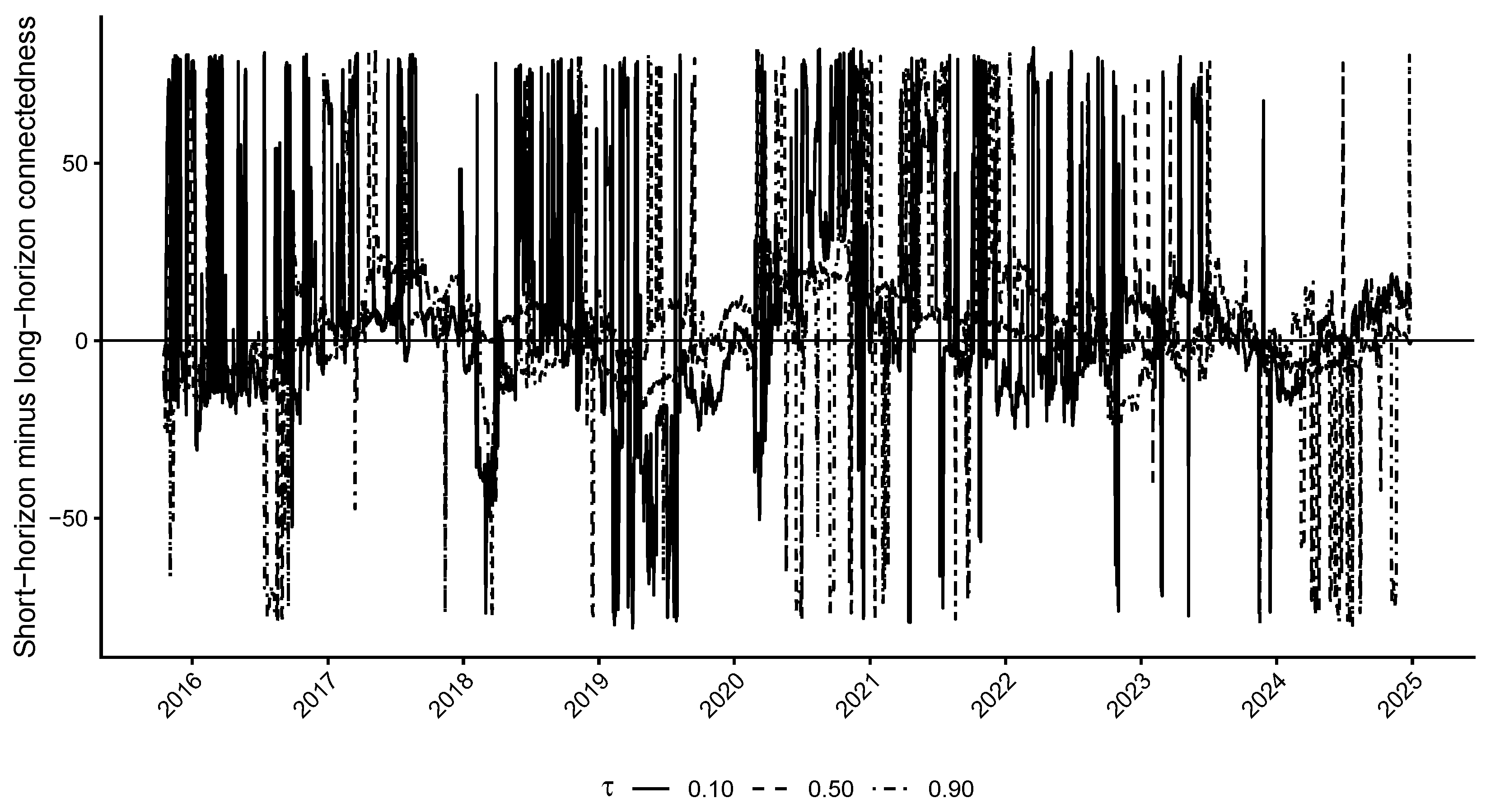
Appendix A.4. Robustness to the Frequency Cutoff in the Quantile–Frequency Analysis
Table A3.
Quantile–frequency connectedness under alternative frequency cutoffs.
Appendix A.5. Stationarity and Persistence Diagnostics
Table A4.
Stationarity and persistence diagnostics.
Appendix A.6. Robustness to Lagged Changes in Connectedness
Table A5.
Robustness to lagged changes in connectedness.
Appendix A.7. Sensitivity to the Newey–West Bandwidth
Table A6 examines whether inference for the main climate risk coefficients is sensitive to the bandwidth used to construct the Newey–West HAC covariance matrix. We consider bandwidths of 5, 20, 50, 100, and 199 trading days. The coefficient estimates are unchanged across bandwidth choices because the underlying OLS specifications are identical; only the estimated standard errors and associated significance levels vary.
Table A6.
Sensitivity to alternative Newey–West bandwidths.
The negative association between physical risk and changes in total connectedness remains statistically significant at the 5% level under all bandwidth choices. The positive association between transition risk and short-horizon connectedness is also qualitatively stable, although its statistical significance is stronger under the longer bandwidth used in the baseline specification. The short-minus-long coefficient for transition risk is less precisely estimated and reaches the 10% significance level only for the longer bandwidth choices. These results support the qualitative interpretation of the baseline estimates while also indicating that inference for the transition risk frequency effects is somewhat sensitive to the treatment of serial dependence.
Appendix A.8. Additional Robustness Checks for the Climate Risk Regressions
Table A7 reports additional robustness checks for the regression explaining daily changes in total connectedness. Panel A considers alternative treatments of influential observations and extreme periods, while Panel B estimates transition and physical risk separately.
The physical risk coefficient remains negative across all specifications. It is statistically significant in the baseline model, when March and April 2020 are excluded, when the dependent variable is winsorized, and when physical risk is entered without transition risk. However, its magnitude declines and statistical significance disappears after observations with absolute studentized residuals greater than three are removed. The physical risk result should therefore be viewed as economically meaningful but not completely insensitive to influential observations.
The transition risk coefficient in the total connectedness regression remains statistically insignificant across these specifications. Moreover, the low variance inflation factors in the baseline regression indicate that the absence of a significant transition risk coefficient for total connectedness is not attributable to severe multicollinearity between the two climate risk measures. Taken together with the frequency-specific results in the main text, these findings reinforce the interpretation that transition risk is associated primarily with the horizon composition of connectedness rather than with its aggregate daily change.
Table A7.
Robustness of the climate risk regression.
Appendix A.9. Robustness of the Climate Risk Regressions to an Alternative Frequency Cutoff
Table A8.
Climate risk regressions with an alternative five-trading-day frequency cutoff.
References
- Bolton, P.; Kacperczyk, M. Do Investors Care about Carbon Risk? J. Financ. Econ. 2021, 142, 517–549. [Google Scholar] [CrossRef] [Scilit]
- Bolton, P.; Kacperczyk, M. Global Pricing of Carbon-Transition Risk. J. Financ. 2023, 78, 3677–3754. [Google Scholar] [CrossRef] [Scilit]
- Engle, R.F.; Giglio, S.; Kelly, B.; Lee, H.; Stroebel, J. Hedging Climate Change News. Rev. Financ. Stud. 2020, 33, 1184–1216. [Google Scholar] [CrossRef] [Scilit]
- Hong, H.; Karolyi, G.A.; Scheinkman, J.A. Climate Finance. Rev. Financ. Stud. 2020, 33, 1011–1023. [Google Scholar] [CrossRef] [Scilit]
- Pástor, V.; Stambaugh, R.F.; Taylor, L.A. Sustainable Investing in Equilibrium. J. Financ. Econ. 2021, 142, 550–571. [Google Scholar] [CrossRef] [Scilit]
- Ilhan, E.; Sautner, Z.; Vilkov, G. Carbon Tail Risk. Rev. Financ. Stud. 2021, 34, 1540–1571. [Google Scholar] [CrossRef] [Scilit]
- Reboredo, J.C. Is There Dependence between Oil and Renewable Energy Stock Prices? Energy Econ. 2015, 48, 32–45. [Google Scholar] [CrossRef] [Scilit]
- Reboredo, J.C.; Rivera-Castro, M.A.; Ugolini, A. Wavelet-based test of co-movement and causality between oil and renewable energy stock prices. Energy Econ. 2017, 61, 241–252. [Google Scholar] [CrossRef] [Scilit]
- Bouri, E.; Iqbal, N.; Klein, T. Climate policy uncertainty and the price dynamics of green and brown energy stocks. Financ. Res. Lett. 2022, 47, 102740. [Google Scholar] [CrossRef] [Scilit]
- Naeem, M.A.; Sadorsky, P.; Karim, S. Sailing across climate-friendly bonds and clean energy stocks: An asymmetric analysis with the Gulf Cooperation Council Stock markets. Energy Econ. 2023, 126, 106911. [Google Scholar] [CrossRef] [Scilit]
- Umar, Z.; Kenourgios, D.; Papathanasiou, S. The static and dynamic Connectedness of environmental, social, and governance investments: International evidence. Econ. Model. 2020, 93, 112–124. [Google Scholar] [CrossRef] [Scilit] [PubMed]
- Diebold, F.X.; Yilmaz, K. Better to Give than to Receive: Predictive Directional Measurement of Volatility Spillovers. Int. J. Forecast. 2012, 28, 57–66. [Google Scholar] [CrossRef] [Scilit]
- Diebold, F.X.; Yilmaz, K. On the Network Topology of Variance Decompositions: Measuring the Connectedness of Financial Firms. J. Econom. 2014, 182, 119–134. [Google Scholar] [CrossRef] [Scilit]
- White, H.; Kim, T.H.; Manganelli, S. VAR for VaR: Measuring Tail Dependence Using Multivariate Regression Quantiles. J. Econom. 2015, 187, 169–188. [Google Scholar] [CrossRef] [Scilit]
- Ando, T.; Greenwood-Nimmo, M.; Shin, Y. Quantile Connectedness: Modeling Tail Behavior in the Topology of Financial Networks. Manag. Sci. 2022, 68, 2401–2431. [Google Scholar] [CrossRef] [Scilit]
- Adrian, T.; Brunnermeier, M.K. CoVaR. Am. Econ. Rev. 2016, 106, 1705–1741. [Google Scholar] [CrossRef] [Scilit]
- Baruník, J.; Křehlík, T. Measuring the Frequency Dynamics of Financial Connectedness and Systemic Risk. J. Financ. Econom. 2018, 16, 271–296. [Google Scholar] [CrossRef] [Scilit]
- Antonakakis, N.; Chatziantoniou, I.; Gabauer, D. Refined Measures of Dynamic Connectedness Based on Time-Varying Parameter Vector Autoregressions. J. Risk Financ. Manag. 2020, 13, 84. [Google Scholar] [CrossRef] [Scilit]
- Demirer, R.; Diebold, F.X.; Liu, L.; Yilmaz, K. Estimating Global Bank Network Connectedness. J. Appl. Econom. 2018, 33, 1–15. [Google Scholar] [CrossRef] [Scilit]
- Alessi, L.; Ossola, E.; Panzica, R. What Greenium Matters in the Stock Market? The Role of Greenhouse Gas Emission and Environmental Disclosures. J. Financ. Stab. 2021, 54, 100869. [Google Scholar] [CrossRef] [Scilit]
- Pham, L. Is It Risky to Go Green? A Volatility Analysis of the Green Bond Market. J. Sustain. Financ. Invest. 2016, 6, 263–291. [Google Scholar] [CrossRef] [Scilit]
- Mhadhbi, M. The Interconnected Carbon, Fossil Fuels, and Clean Energy Markets: Exploring Europe and China’s Perspectives on Climate Change. Financ. Res. Lett. 2024, 62, 105185. [Google Scholar] [CrossRef] [Scilit]
- Cong, O.; Xue, H. Volatility Spillovers between Energy Market and Carbon Market: The TVP-SV-VAR and DCC-GARCH-Connectedness Approaches. J. Environ. Manag. 2025, 396, 128055. [Google Scholar] [CrossRef] [Scilit] [PubMed]
- Dong, F.; Li, Z.; Huang, Z.; Liu, Y. Extreme Weather, Policy Uncertainty, and Risk Spillovers between Energy, Financial, and Carbon Markets. Energy Econ. 2024, 137, 107761. [Google Scholar] [CrossRef] [Scilit]
- Baker, S.R.; Bloom, N.; Davis, S.J. Measuring Economic Policy Uncertainty. Q. J. Econ. 2016, 131, 1593–1636. [Google Scholar] [CrossRef] [Scilit]
- Gavriilidis, K. Measuring Climate Policy Uncertainty. SSRN Working Paper No. 3847388, 2021. Available online: https://ssrn.com/abstract=3847388 (accessed on 10 July 2026). [CrossRef] [Scilit]
- Bua, G.; Kapp, D.; Ramella, F.; Rognone, L. Transition versus Physical Climate Risk Pricing in European Financial Markets. Eur. J. Financ. 2024, 30, 2076–2110. [Google Scholar] [CrossRef] [Scilit]
- Pankratz, N.; Bauer, R.; Derwall, J. Climate Change, Firm Performance, and Investor Surprises. Manag. Sci. 2023, 69, 7151–7882. [Google Scholar] [CrossRef] [Scilit]
- Koenker, R.; Bassett, G. Regression Quantiles. Econometrica 1978, 46, 33–50. [Google Scholar] [CrossRef] [Scilit]
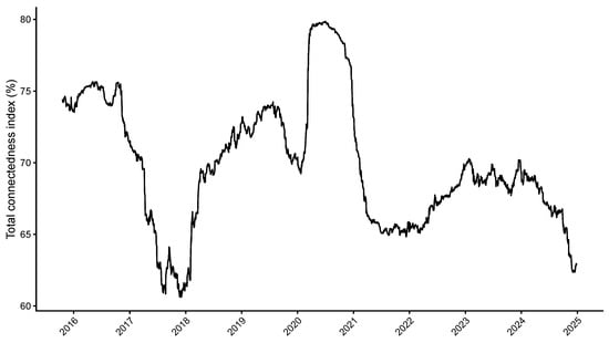
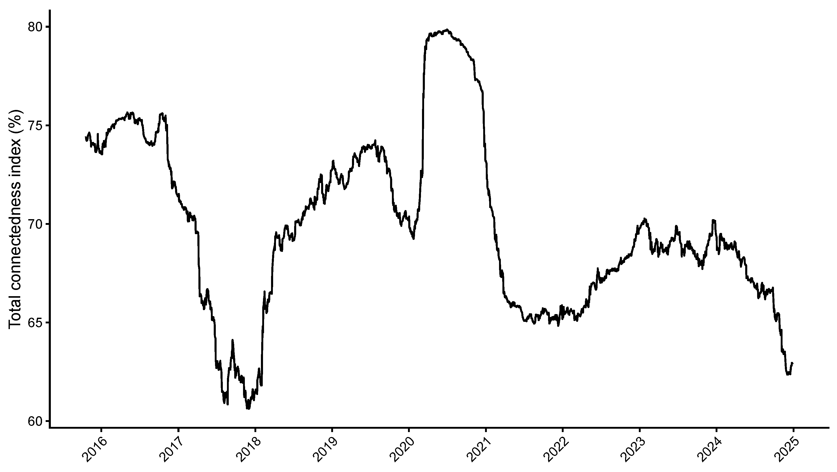
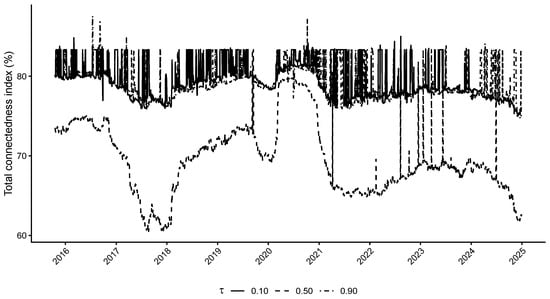
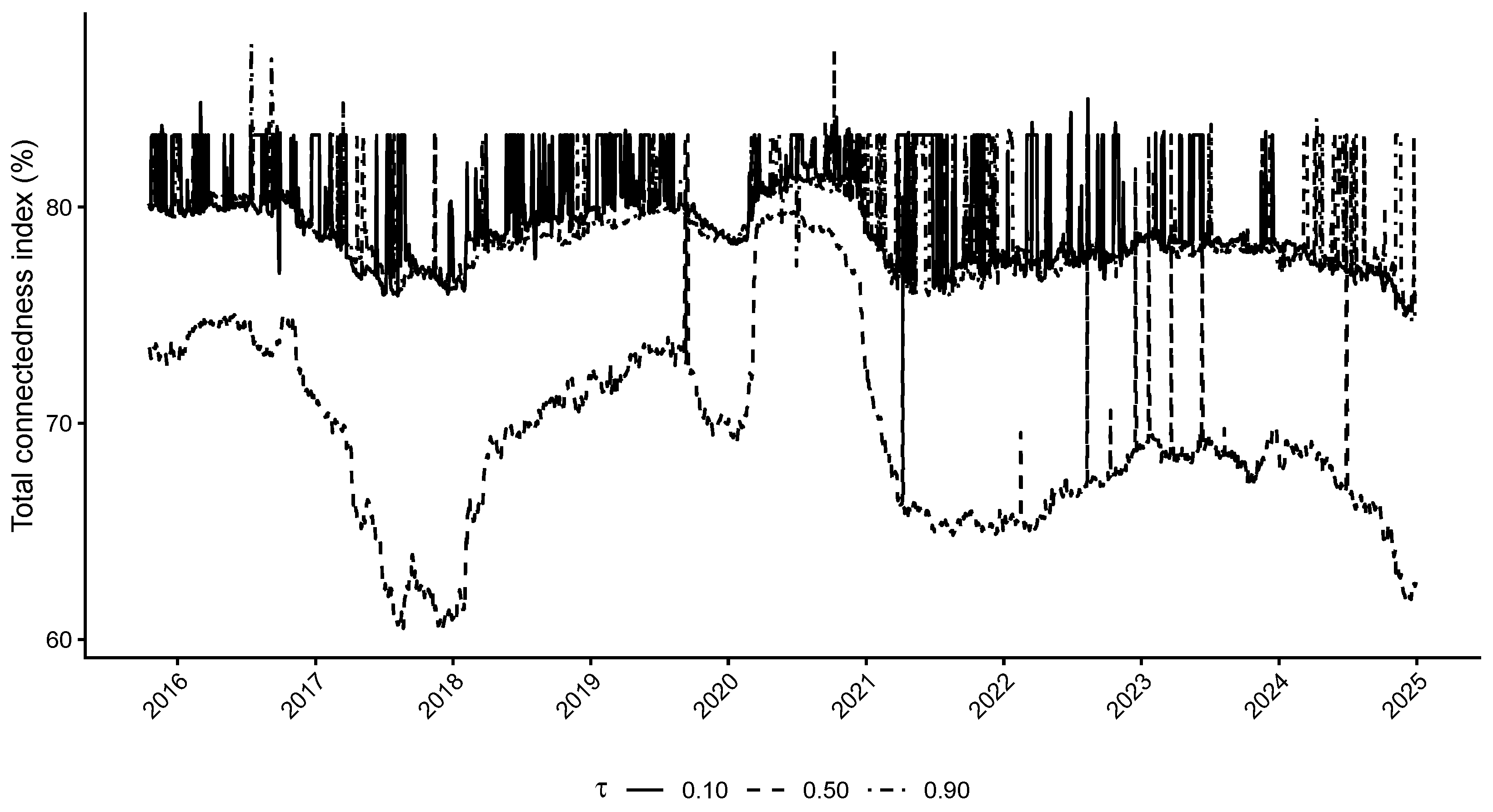
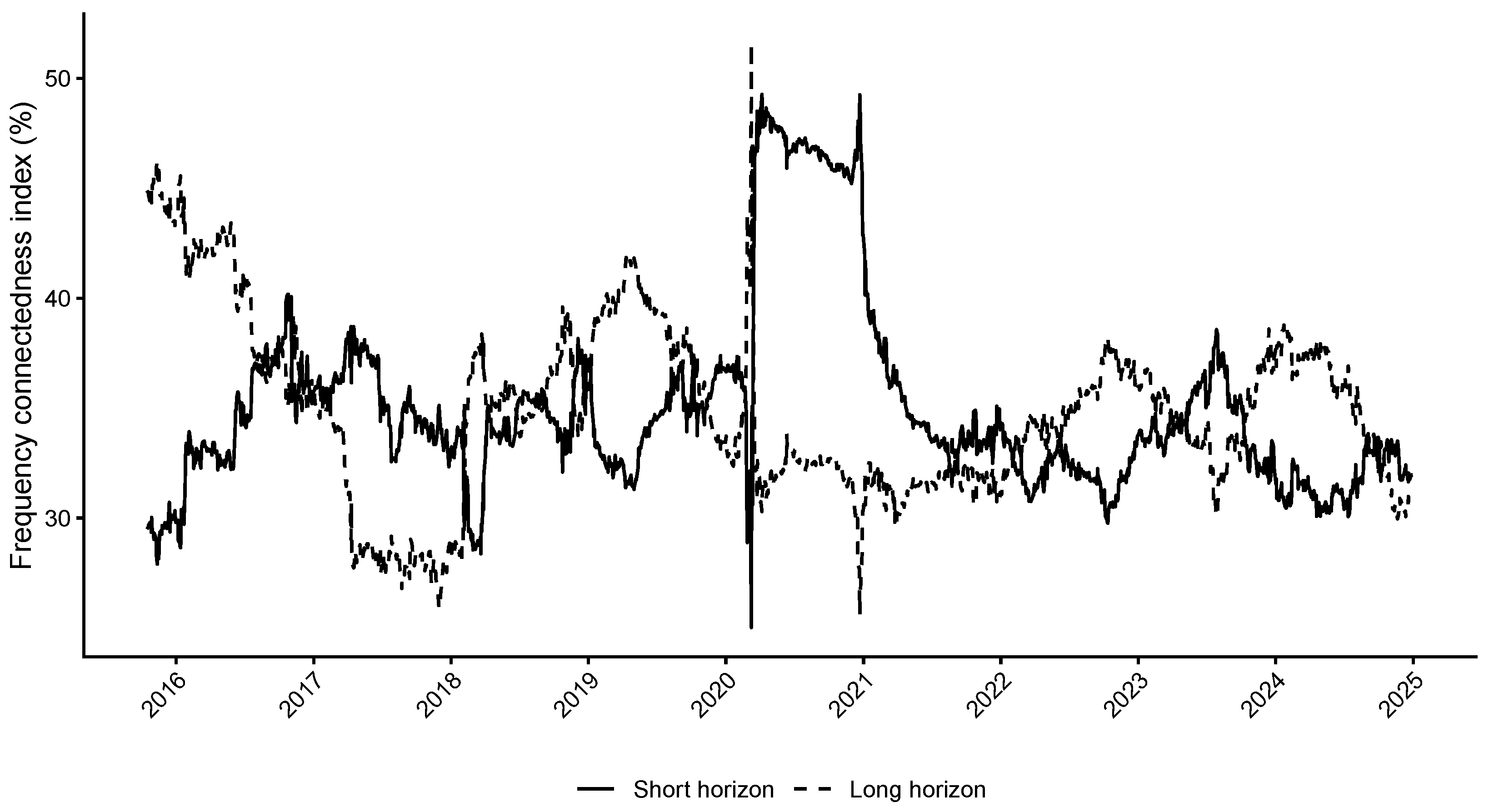
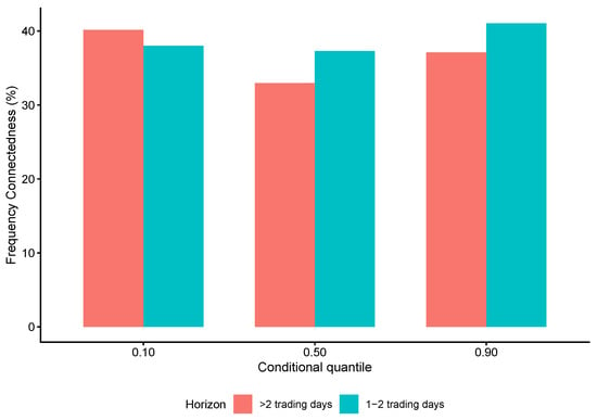
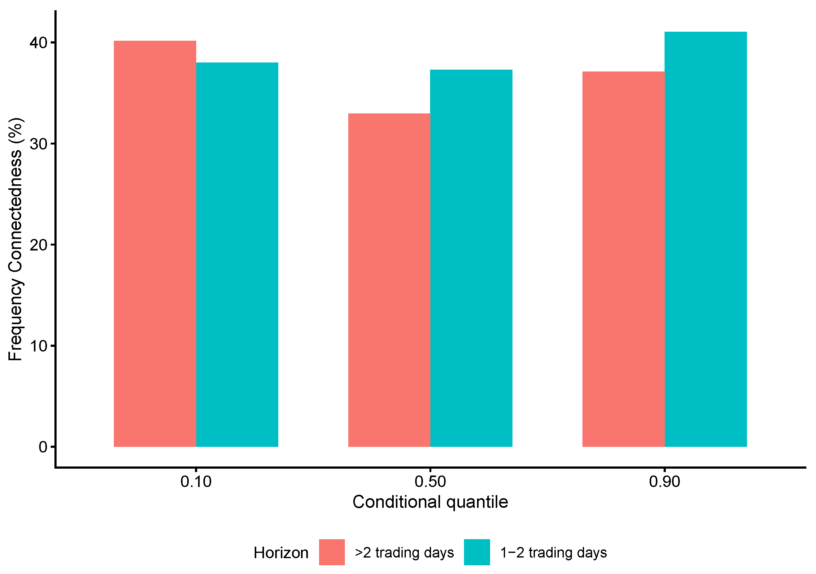

Disclaimer/Publisher’s Note: The statements, opinions and data contained in all publications are solely those of the individual author(s) and contributor(s) and not of MDPI and/or the editor(s). MDPI and/or the editor(s) disclaim responsibility for any injury to people or property resulting from any ideas, methods, instructions or products referred to in the content. |
© 2026 by the author. Licensee MDPI, Basel, Switzerland. This article is an open access article distributed under the terms and conditions of the Creative Commons Attribution (CC BY) license.