


Abstract
This study proposes a hybrid analytical–numerical method for accurately extracting five physically meaningful single-diode-model (SDM) parameters from measured illuminated I–V data. Five experimental data points are randomly selected to construct a system of five nonlinear implicit SDM equations. Hejri’s analytical method provides physically meaningful initial estimates, and an improved five-dimensional Newton–Raphson method is then used to solve the resulting equation system. When accurate characteristic-point data are unavailable, a metaheuristic fitting procedure is employed to determine the characteristic parameters required by initialization. The method is evaluated on the RTC cell, PWP 201 module, TOPCon cell, and TOPCon module and benchmarked against six state-of-the-art techniques: Ghani’s method, Hejri’s method, Kumar’s method, the artificial ecosystem-based optimization (AEO) algorithm, Phang’s method, and Villalva’s method. The proposed method achieves RMSE values of 8.31 × 10⁻⁴, 2.10 × 10⁻³, 2.40 × 10⁻², and 2.36 × 10⁻² A, respectively, consistently yielding the lowest RMSE among the four hybrid analytical–numerical methods. Its RMSE values are only 0.5–7.5% above the corresponding minima obtained by AEO. Moreover, in the equation-solving step, the proposed solver is approximately 30–2954 times faster than Ghani’s method and achieves higher convergence rates for three of the four devices. These results demonstrate that the proposed method enables accurate and efficient extraction of physically meaningful SDM parameters.
1. Introduction
Driven by the global energy transition and the pursuit of carbon neutrality, solar photovoltaic (PV) power generation has emerged as one of the fastest-growing renewable energy technologies. It has already occupied a significant share in the global energy supply system [1,2]. The large-scale application of PV power generation systems requires performance simulation [3], power generation forecasting [4], system optimization design [5], maximum power point tracking [6], performance degradation analysis [7], and fault diagnosis [8]. All these tasks rely on the accurate modeling of the current–voltage (I–V) characteristics of solar cells or PV modules. To this end, single-diode models (SDM), double-diode models (DDM), and even triple-diode models (TDM) have been developed to describe the I–V characteristics of solar cells or PV modules [9], with the SDM and DDM being the most widely accepted and recognized models [10]. Since the SDM can well balance the simplicity and accuracy of the model—predicting the I–V characteristics of solar cells or PV modules fairly accurately while maintaining a relatively simple mathematical formula—it is likely the most widely used model at present [10,11]. However, the SDM is a transcendental and implicit equation containing multiple unknown parameters. Specifically, it includes five SDM parameters, namely, the photogenerated current (Iph), the diode reverse saturation current (I0), the diode ideality factor (n), the shunt resistance (Rsh), and the series resistance (Rs). In practice, manufacturers rarely disclose the values of these SDM parameters. Instead, they typically only provide limited information such as illuminated I–V characteristic data of the solar cells or modules, including power conversion efficiency (PCE), open-circuit voltage (Voc), short-circuit current (Isc), maximum power point voltage (Vm), maximum power point current (Im), and fill factor (FF). Therefore, how to accurately extract the SDM parameters of solar cells or PV modules from the measured illuminated I–V characteristics has long been an important research topic that PV researchers have to address.
Regarding the SDM parameter extraction from solar cells or PV modules, analytical methods, numerical methods, and meta-heuristic algorithms (also named intelligent optimization algorithms) have been developed. The analytical method applies the SDM model to three key points of the measured I–V characteristics (the Isc, Voc, and maximum power point) to obtain a set of nonlinear equations. Through a series of simplifying assumptions and complex mathematical derivations, the multiple nonlinear implicit equations satisfied by the SDM parameters are simplified into analytical expressions that allow the SDM parameters to be directly calculated from the characteristic parameter values. The analytical method proposed by Phang et al. is probably the most frequently used analytical method with the highest parameter extraction accuracy [12]. In Phang’s analytical method [13], the authors gave formulas for calculating SDM parameters using six characteristic parameter values (Voc, Isc, Vm, Im, Rs0, and Rsh0). Here, Rs0 and Rsh0 correspond to the negative reciprocals of the slopes of the measured I–V curve at Voc and Isc, respectively. Analytical methods have advantages such as being simple, direct, and fast. However, due to the introduction of simplifying assumptions, the accuracy of the extracted SDM parameters is limited. They are often used to provide initial values of SDM parameters for numerical methods [14]. For details about the research on SDM parameter extraction using analytical methods, please see review articles [14,15,16]. Numerical methods can be divided into iterative methods based on trial and error and numerical calculation methods for solving a system of nonlinear equations. The method proposed by Villalva et al. is likely the most widely used iterative approach [17]. In this method, it is assumed that Iph = Isc, the diode ideality factor n is determined by the type of PV module (for monocrystalline silicon cells, n = 1.2), I0 is calculated by an approximate formula obtained from the analytical method, while the remaining two parameters (Rs and Rsh) are determined by the iterative method. Specifically, an initial value of Rs is given (typically Rs = 0). Enter the loop, the value of Rsh is first calculated by a prescribed formula, and then the simulated maximum power is calculated and compared with the measured maximum power. When the difference between the two is greater than the allowable error, Rs is increased by a very small step (e.g., 0.0001). Enter the next loop, …, until the difference between the simulated and the measured maximum power is less than the allowable error; exit the loop. The resulting Rs and Rsh are regarded as the final solution [18]. Obviously, the SDM parameters determined by this method can ensure that the simulated I–V curve passes through the measured maximum power point. Comprehensive reviews of research on SDM parameter extraction using numerical iterative methods can be found in Refs. [17,19]. Another numerical method is to obtain SDM parameters by solving a system of nonlinear equations using the Newton–Raphson (N–R) method [20] or the Levenberg–Marquardt (L–M) algorithm [21]. Although these methods can yield accurate SDM parameters, they are highly sensitive to the setting of initial values, because both N–R and L–M algorithms are numerical iterative methods based on gradient descent. If the initial values are set inappropriately, these methods will fail to converge [20,22,23]. Moreover, these methods involve complex solution procedures and generally require strong programming skills or the use of powerful mathematical software tools such as MATLAB.
In recent years, more and more researchers have employed meta-heuristic algorithms for extracting PV model parameters [10,24,25]. In fact, meta-heuristic algorithms were developed to solve complex nonlinear optimization problems frequently encountered in engineering practice. To extract PV model parameters using meta-heuristic algorithms, the parameter extraction task must first be formulated as an optimization problem. A common approach is to define the root-mean-square error (RMSE) between the simulated and measured I–V characteristics as the objective function and then identify the optimal model parameters by minimizing the RMSE. In contrast to analytical or numerical techniques that rely on a limited number of I–V data points, meta-heuristic algorithms use complete measured I–V dataset for parameter identification. Furthermore, meta-heuristic algorithms simply employ randomly generated numbers as starting points, entirely eliminating the need for strict initial value settings. Owing to their flexibility, meta-heuristic algorithms are well suited for solving strongly nonlinear and high-dimensional optimization problems, and they are attractive because of their global search ability, relatively high accuracy, and user-friendly implementation. Nevertheless, their application to PV model parameter extraction still faces several limitations. Specifically, search bound for each target parameter need to be specified by user before optimization, and the obtained solutions may vary from one run to another because of their stochastic nature. In addition, premature convergence and trapping in local optima can also occur. More importantly, a parameter set that produces the lowest RMSE may not always be physically meaningful, even if it provides a good numerical fit to the measured I–V curve.
From above introduction to the methods for extracting SDM parameters, it is not difficult to see that analytical methods have limited extraction accuracy because they introduce simplifying assumptions. To reduce the number of unknown parameters, numerical iterative methods often adopt approximate expressions derived from analytical approaches. In addition, the determination of certain parameters in numerical iterative methods is based on trial and error, which can only ensure that the obtained parameters satisfy the specified condition. When meta-heuristic algorithms are adopted for SDM parameter identification, the model parameters are typically initialized in a random and independent manner and subsequently updated following the search strategy of the algorithm. The parameter set that yields the lowest RMSE between the simulated and experimental I–V curves is selected as the optimal solution. Therefore, this method is essentially a curve fitting method. Previous work [23] has pointed out that fitting-based parameter extraction may lead to incorrect parameter values, since different PV model parameters can vary simultaneously during the optimization process to improve the overall fit to the measured I–V curves. As a result, compensation effects among parameters may introduce significant errors into the extracted results. Moreover, it has been reported that numerous parameter combinations are capable of reproducing the same measured I–V curve [26]. Consequently, it remains difficult to determine which extracted parameter set is physically meaningful.
Solving a system of nonlinear equations by the numerical calculation method seems to be the only way at present to obtain accurate and physically meaningful SDM parameters. However, this method requires setting appropriate initial values for the SDM parameters. If the initial values are set improperly, the numerical method will fail to converge. For this reason, hybrid methods combining analytical and numerical methods have been proposed. In these methods, the analytical method provides the initial values of the SDM parameters for the numerical method, and the numerical method obtains accurate and physically meaningful SDM parameters by solving the system of nonlinear equations. In this research field, Ghani et al. [27] substituted coordinates of five data points on the measured I–V curve into the explicit equation of the SDM expressed by the Lambert W (LW) function to establish five equations in 2014. Then, they used the five-dimensional N–R method to simultaneously solve the five equations to obtain the five SDM parameters. It should be noted that Ghani et al. further simplified the formulas given by Phang’s analytical method and then calculated the initial values of the five SDM parameters using these formulas and four characteristic parameter values (Voc, Isc, Rs0 and Rsh0). Also in 2014, Hejri et al. [20] applied the SDM equation to three key points on the measured I–V characteristics to obtain three equations. Next, they obtained the fourth equation based on the condition that the derivative of power with respect to voltage is zero at the maximum power point. By eliminating Iph, three equations relating the four SDM parameters (I0, Rs, Rsh, and n) were obtained. Then, the fourth equation was established by using the negative reciprocal of the slope of the I–V curve at the Isc being equal to Rsh0 and assuming Rsh = Rsh0. After that, the four-dimensional N–R method was used to simultaneously solve these four equations to obtain the four SDM parameters. Finally, Iph was calculated from these four SDM parameters and Voc. It should be noted that Hejri et al. provided a new analytical method for calculating SDM parameters, which can obtain high-quality initial values of the SDM parameters by using only the coordinates of three key points (Voc, Isc, Im and Vm) provided by the manufacturer. In 2017, Kumar et al. [21] applied the SDM equation to the three key points to obtain three equations. The other two equations correspond to the derivative of power with respect to voltage at the maximum power point being zero, and the negative reciprocal of the slope of the I–V curve at the Isc being equal to Rsh0 with the assumption Rsh = Rsh0, respectively, which is similar to the approach of Hejri et al. Then, MATLAB’s fsolve function embedded with the L–M algorithm was used to simultaneously solve these five nonlinear equations to obtain the five SDM parameters. It should be noted that Kumar et al. gave a new analytical method different from that of Hejri et al. to calculate SDM parameters. This method also uses only limited information provided by the manufacturer (Voc, Isc, Im, and Vm) to calculate the initial values of SDM parameters that can ensure the convergence of the numerical method.
The aforementioned hybrid analytical–numerical methods all have their own shortcomings. Ghani et al. used the five-dimensional N–R method to solve five explicit equations of the SDM expressed by the LW function. The Jacobian matrix needs to be solved in each iteration. Among the 25 elements of the Jacobian matrix, 20 elements require the calculation of the LW function. However, the LW function is the inverse function of f(x) = x·ex, and its calculation consumes significant computational resources. When using Ghani’s method to extract SDM parameters, we found that it suffers from heavy computational burden, long computation time, slow convergence and difficulty in converging to ideal parameter values. Moreover, in the system of equations solved by Hejri’s or Kumar’s method, one equation includes the approximation of Rsh = Rsh0, which would affect parameter extraction accuracy. In addition, both methods use the coordinates or derivatives of three key points to establish the equations. If the measured data contains noise, the system of equations established by these three noisy characteristic points may have no solution. This occurs when no I–V curve conforming to the same SDM equation can strictly pass through the three noisy characteristic points.
To address the existing problems of hybrid analytical–numerical methods, this paper proposes a new method for accurately determining five SDM parameters with physical meaning from measured illuminated I–V characteristic data of a solar cell or a PV module. In this method, five data points of the measured I–V data are first randomly selected to construct five nonlinear implicit equations that the SDM parameters strictly satisfy. Then, the analytical method given by Hejri et al. is used to calculate the initial values of the SDM parameters. Finally, an improved five-dimensional N–R method is used to solve the system of five nonlinear implicit equations, so as to uniquely determine the accurate and physically meaningful SDM parameters of the solar cell or PV module. The innovation of this approach lies in the following: (1) The improvement of the multidimensional N–R method. By introducing a step size factor less than 1 (such as k0 = 0.01) into the iterative formula, the finer values can be taken during the iteration process, which significantly improves the convergence capability of the numerical method. (2) The use of high-quality initial values of SDM parameters. If the accurate coordinates of three key points (Voc, Isc, Im, and Vm) are unavailable, a meta-heuristic algorithm needs to be employed to fit the measured I–V data to obtain the best-fit I–V curve with the minimum RMSE. Then, by solving the related equations, the exact coordinates of three key points on the best-fit curve are determined. Finally, these accurate characteristic parameter coordinates are introduced into Hejri’s analytical formulas to derive reliable initial estimates. (3) We randomly select five data points from the measured I–V characteristics to construct a system of five nonlinear implicit equations, with the five SDM parameters treated as unknowns. Provided that the five randomly selected data points satisfy the same SDM equation, the proposed method can uniquely determine accurate and physically meaningful SDM parameters by numerically solving the resulting system of equations using an improved five-dimensional N–R method. The proposed method was applied to the French RTC cell and Photowatt PWP 201 module, which are often used as benchmark devices for parameter extraction, as well as to the TOPCon cell and TOPCon module, which are mainstream products in the current PV market. The SDM parameter extraction results were compared with other six state-of-the-art methods (Ghani’s method [27], Hejri’s method [20], Kumar’s method [21], the artificial ecosystem-based optimization (AEO) algorithm [28], Phang’s method [13], and Villalva’s method [18]). The results show that the proposed method is capable of extracting accurate and physically meaningful SDM parameters from all four PV devices.
2. Principles and Methods
2.1. Single-Diode Models (SDMs) of a Solar Cell and a PV Module
Figure 1 presents the equivalent circuit diagram of the SDM for a solar cell. As illustrated in Figure 1, the SDM comprises a constant current source Iph, a diode D, a shunt resistance Rsh, and a series resistance Rs.
Figure 1.
Equivalent circuit diagram of the single-diode model for a solar cell.
The SDM equation of a solar cell can be derived from Figure 1 and Kirchhoff’s law:
where I is the current across the load (A), Iph is the photogenerated current (A), I0 is the reverse saturation current of diode D (A), n is the ideality factor of diode D, V is the voltage across the load (V), Rs is the series resistance (Ω), Rsh is the shunt resistance (Ω), and Vth is the thermal voltage (V), which can be written as
where k is the Boltzmann constant (J·K−1), T is the absolute temperature of the solar cell (K), and q is the elementary charge (C).
To meet power demand, a PV module typically consists of multiple solar cells, which are first connected in series to form a cell string, and then several cell strings connected in parallel to form a module. Assuming that all solar cells in the module possess identical SDM parameters (Iph, I0, Rs, Rsh, n), and let Ns represent the number of cells connected in series in a string, and Np denote the number of strings connected in parallel in the PV module, then, the equivalent circuit diagram of the SDM for the PV module can be given by Figure 2.
Figure 2.
Equivalent circuit diagram of the single-diode model for a photovoltaic module.
The SDM equation of a PV module can be derived from Figure 2 and Kirchhoff’s law
Comparing Equations (1) and (3), it is evident that Equation (3) can be obtained by substituting Iph, I0, n, Rs and Rsh in Equation (1) with IphNp, I0Np, nNs, RsNs/Np and RshNs/Np, respectively.
2.2. Equations That Link the SDM Parameters and Characteristic Parameter Values of I–V Characteristic Curve of a Solar Cell and a PV Module
The derivation of the six equations relating the five SDM parameters (Iph, I0, Rs, Rsh and n) of a solar cell and the characteristic parameter values (Voc, Isc, Im, Vm, Rs0, Rsh0) of the I–V characteristics is given below.
At the open-circuit condition, V = Voc and I = 0. Substituting these values into the SDM equation of the solar cell yields
At the short-circuit condition, V = 0 and I = Isc. Substituting these values into Equation (1) gives
At the maximum power point, V = Vm and I = Im. Substituting these values into Equation (1) yields
Taking the derivative of both sides of Equation (1) with respect to V gives
At the maximum power point,
Substituting Equation (8) into Equation (7) gives
From Ref. [13], the slope of the I–V curve at the open-circuit voltage is equal to the negative reciprocal of Rs0, i.e., . Combining this expression with Equation (7) yields
From Ref. [13], the slope of the I–V curve at the short-circuit current is equal to the negative reciprocal of Rsh0, i.e., . Incorporating this expression into Equation (7) gives
Equations (4)–(6) and (9)–(11) are the six equations relating the five SDM parameters to the characteristic parameter values of the I–V characteristic curve.
Similarly, the six equations relating the five SDM parameters (Iph, I0, Rs, Rsh, and n) of a PV module and the characteristic parameter values (Voc, Isc, Vm, Im, Rs0, Rsh0) of the I–V characteristic curve can be derived. Because no approximations were introduced in the derivation, the above equations are strictly valid.
2.3. One- and Multi-Dimensional Newton–Raphson Methods
The one-dimensional N–R method is a numerical iteration approach for solving a nonlinear equation f(x) = 0. Its iteration formula is:
where is the current value of , is the function value of the , is the derivative value of , and is the next iterative value of x. When using the one-dimensional N–R method to solve the nonlinear equation , an initial value needs to be provided. Then, iteration is carried out using Equation (12) until is sufficiently close to zero. Here, is treated as the root of the nonlinear equation. It should be mentioned that when SDM parameters of a solar cell or a PV module are given, this work utilizes the one-dimensional N–R method to solve Equation (1) or Equation (3) to obtain the accurate simulated current (Isimulated), thus RMSE between the simulated and measured I–V characteristics.
The N–R method can be generalized to its multidimensional form for solving a system of multiple nonlinear equations. The corresponding iterative formula is given as follows:
where is a vector containing the current values of all unknown variables. is a vector composed of function values for each function in the current system of equations. is the Jacobian matrix containing the partial derivatives of each function with respect to each unknown variable. is a vector consisting of the values of the unknown variables for the next iteration. When using the multi-dimensional N–R method to solve a nonlinear equation system, a vector containing the initial values of all unknown variables needs to be provided. Then, iteration is performed using Equation (13) until the sum of the absolute value of each function in is sufficiently close to zero. At this time, is taken as the solution of the nonlinear equation set.
2.4. Extraction of Five SDM Parameters Using the Five-Dimensional Newton–Raphson Method
This paper utilizes five data points from the measured I–V characteristics of a solar cell or a PV module to construct a system of five SDM equations. The system can be written as
For solar cells, Fx(Ix,Vx) in Equation set (14) takes the following form:
For PV modules, Fx(Ix,Vx) in the equation set (14) has the form:
The vector X consisting of five SDM parameters (Iph, I0, Rs, Rsh, and n) can be expressed as
Equation (13) can be rewritten in matrix form:
When applying the five-dimensional N–R method to solve the nonlinear equation set (14), we introduced a step-size factor smaller than 1 (e.g., k0 = 0.01) to Equation (13). Thus, the practically used iteration formula is
This adjustment allows the finer values of SDM parameters to be taken during the iteration, which can ensure stable convergence of the five-dimensional N–R method when solving the nonlinear equation set (14). However, when directly using Equation (13) for iteration, the five-dimensional N–R method often fails to converge. This is mainly because during the iteration, some SDM parameters calculated by Equation (13) may jump out of physically meaningful ranges (e.g., become negative), which causes subsequent iterations to deviate more from the true solution, leading to convergence failure.
2.5. Initialization of the Five SDM Parameters
When using the five-dimensional N–R method to solve the nonlinear equation set (14), it is necessary to provide high-quality initial values of five SDM parameters. Otherwise, the method will fail to converge. In this paper, we use the analytical method provided by Hejri et al. [20] to calculate the initial values of SDM parameters.
For solar cells, the formulas for calculating the initial values of SDM parameters are as follows:
For PV modules, the equations for calculating the initial values of SDM parameters are as below:
2.6. Accurate Determination of Characteristic Parameter Values from the Measured I–V Curve
If the accurate coordinates of the three key points (i.e., Isc, Voc, Im, Vm) are unavailable, one has to determine them first. Recognizing that experimental I–V measurements are typically subject to noise, we utilize a meta-heuristic algorithm to fit the measured illuminated I–V characteristics to achieve the best-fit I–V curve. Then, by solving relevant equations, we obtain the accurate characteristic parameter values (Isc, Voc, Im, Vm, Rs0, and Rsh0) on the best-fit curve. In particular, utilizing the RMSE as the objective function (Equation (30)), which quantifies the discrepancy between the simulated current (Isimulated) and the measured current (Imeasured) across all data points:
We employ a meta-heuristic algorithm to minimize the RMSE, thereby identifying the optimal SDM parameters that yield the best-fit I–V curve. Subsequently, we utilize the vpasolve function in MATLAB to solve Equation (4) for Voc, Equation (10) for Rs0, Equation (5) for Isc, Equation (11) for Rsh0, and Equations (6) and (9) for Im and Vm. A similar procedure is applied to derive the characteristic parameter values (Isc, Voc, Im, Vm, Rs0, and Rsh0) of a PV module. Accurate determination of the coordinates of three characteristic points (Isc, Voc, Im, Vm) enables the reliable estimation for initial values of SDM parameters via Hejri’s method, thereby ensuring the convergence of the improved five-dimensional N–R method in solving equation set (14). Although the proposed method does not require Rs0 and Rsh0, we calculated them solely for the comparison with Ghani’s and Phang’s methods, which depend on these parameters.
2.7. Flowchart for Extracting the Five SDM Parameters Using the Improved Five-Dimensional Newton–Raphson Method
Figure 3 illustrates the procedure for extracting five SDM parameters via the five-dimensional N–R method. First, input the measured illuminated I–V characteristic data and necessary parameters. Second, in cases where the information of the three characteristic points is unavailable, a meta-heuristic algorithm is used to fit the measured I–V data to achieve the optimal SDM parameters that minimizes the RMSE. Subsequently, the exact coordinates of three characteristic points on the resulting best-fit curve can be obtained by solving the relevant equations. Third, use Hejri’s analytical method and the information of three characteristic points (Isc, Voc, Im, Vm) to estimate the initial values of five SDM parameters. After these initialization steps, the main loop starts. First, five points are randomly chosen from the measured I–V dataset to formulate the equation set (14). Then, use the improved five-dimensional N–R method to solve the resulting equation set, utilizing Equation (19) for the iteration. At each iteration, the residual error and the iteration count are checked. When the error tolerance is satisfied, save the solution. When the iteration limit is reached, the process proceeds to the next main loop based on another randomly selected five I–V data points. This procedure is repeated until the total simulation count (max_N) is met.
Figure 3.
Flowchart for obtaining the five SDM parameters by solving the nonlinear equation system via the improved five-dimensional Newton–Raphson method.
3. Results and Discussion
To enable a direct comparison with existing literature, we employed the proposed method to extract SDM parameters from the frequently cited French RTC silicon solar cell (57 mm diameter) and the Photowatt PWP 201 module (36 polycrystalline cells in series). It should be noted that the I–V characteristic data were measured at an irradiance of 1000 W/m2, with temperatures of 33 °C for the RTC cell and 45 °C for the PWP 201 module [29]. Given that the RTC cell and PWP 201 module are based on technologies developed nearly four decades ago, we further applied the proposed method to extract the SDM parameters of a TOPCon cell and module, which represent current mainstream PV technology. The TOPCon cell is a 16-busbar, bifacial, pseudo-square device (182 mm × 182 mm) with an effective area of 330.15 cm2. The TOPCon module is a double-glass type with size of 1134 mm × 2278 mm, which is composed of 144 half-cells (182 mm × 91 mm), with two cell strings connected in parallel and each string containing 72 series-connected half-cells (Ns = 72, Np = 2). I–V characteristics measurements for the TOPCon cell and module were conducted under standard test conditions (25 °C, 1000 W/m2, AM1.5 spectrum). The measured I–V data of the RTC cell, PWP 201 module, TOPCon cell and TOPCon module are given by Supplementary Tables S1–S4, respectively.
To evaluate the proposed method, we compared its parameter extraction performance against six state-of-the-art techniques (Ghani’ method [27], Hejri’ method [20], Kumar’ method [21], AEO algorithm [28], Phang’ method [13], and Villalva’ method [18]) across the four PV devices. To ensure an unbiased and consistent comparison, all seven methods were independently coded on the MATLAB R2025a platform. Furthermore, the simulated currents—essential for determining the RMSE, absolute current error (IAE), and absolute power error (PAE)—were calculated by using the one-dimensional N–R method for all extracted SDM parameters. In this study, the SDM parameters reported for PV modules all correspond to the parameters of a single cell within the module. Owing to its superior parameter extraction performance [30], the AEO algorithm was selected as the representative meta-heuristic technique for estimating SDM parameters. The algorithm was initialized using default settings, with a population size of 50, and a maximum iteration number of 3000 for the RTC cell, 2000 for the PWP 201 module and 5000 for both the TOPCon cell and module, and executed 30 times independently to identify the optimal parameter set. The specific parameter search ranges are listed in Supplementary Table S5. Furthermore, due to lack of manufacturer-supplied information of three characteristic points, the AEO algorithm was utilized to fit the measured I–V data of the four PV devices to obtain the best-fit I–V curves. Subsequently, accurate characteristic parameter values (Isc, Voc, Im, Vm, Rs0, and Rsh0) of the best-fit curves were acquired by solving relevant equations using the vpasolve function in MATLAB. Supplementary Table S6 summarizes the optimal SDM parameters extracted via the AEO algorithm for the four PV devices, along with the six characteristic parameter values. The latter was used by the seven comparative methods. Specifically, all six parameters (Isc, Voc, Im, Vm, Rs0, Rsh0) were utilized by Phang’s method. In contrast, Ghani’s method used only four parameters (Isc, Voc, Rs0, Rsh0), while the proposed method, Hejri’s method, Kumar’s method, and Villalva’s method all employed only the coordinates of three characteristic points (Isc, Voc, Im, Vm).
Supplementary Tables S7–S10 present specific parameter settings used for parameter extraction by the proposed method, Ghani’s method, Hejri’s method and Kumar’s method, respectively. Since the parameter extraction accuracy of the proposed method and Ghani’s method is closely related to the number of five-point sampling, we performed 300,000 samplings on the RTC cell and PWP 201 module, and 1 million samplings on both the TOPCon cell and module in order to explore the limits of parameter extraction accuracy for both methods. These calculations were performed on a server (Intel Xeon E5-2696 V4 CPU@2.20 GHz, 256 GB RAM, with the Linux Ubuntu 25.10 OS). Except for the proposed and Ghani’s methods, the other methods were run on a personal computer (Intel Core i7-12700H CPU@2.10 GHz, 16.0 GB RAM, with the Windows 10 64-bit OS). Unless otherwise specified, for both the proposed method and Ghani’s method, computations involving no more than 100,000 five-point sampling trials were performed on the personal computer, whereas those involving more than 100,000 trials were performed on the server.
3.1. Parameter Extraction Results Obtained from the Four PV Devices Using the Proposed Method
Table 1 presents the high-quality initial values of SDM parameters for the four PV devices, obtained via Hejri’s method using the coordinates of three key points (Isc, Voc, Im, Vm) given by Supplementary Table S6. With these initial values, five data points were randomly selected from the measured I–V characteristics to establish equation set (14), which was then solved by the improved five-dimensional N–R method to achieve five accurate and physically meaningful SDM parameters.
Table 1.
High-quality initial values of SDM parameters for the four PV devices, derived via Hejri’s analytical method.
For the four PV devices investigated, all of which employ diffusion-formed p-n junctions, an extracted parameter set was considered physically valid only if it satisfied Iph > 0, I0 > 0, Rs > 0, Rsh > 0, 1 < n < 2. All extracted parameter sets were first screened against above physical-validity constraints and then ranked by RMSE. For each PV device, the five physically valid parameter sets with the lowest RMSE values are reported in Table 2, together with their RMSE values and the indices of the five selected I–V data points. Notably, for each five-point selection, the proposed method yields a unique parameter set. A clear trend can be seen from Table 2 that, for each device, the top five parameter sets display high stability, with only minor variations. For instance, in the RTC cell, I0 is consistently around 3.0 × 10⁻⁷ A, Rs around 3.7 × 10⁻² Ω, Rsh around 53 Ω, and n around 1.5, while RMSE values are all below 8.48 × 10⁻⁴ A. Similarly, for the PWP 201 module, TOPCon cell, and TOPCon module, the parameter distributions are also narrow. This consistency demonstrates that the proposed method is robust to the specific choice of the five I–V data points among the five best selections.
Table 2.
Five physically valid SDM parameter sets with the lowest RMSE values for each of the four PV devices, together with the corresponding selected data-point indices.
To facilitate a performance comparison between the 55 mm diameter French RTC cell and the 330.15 cm2 TOPCon cell, we calculated the area-normalized dark saturation current density (J0), series resistance (Rs) and shunt resistance (Rsh) for both devices. The extracted parameter ranges for the TOPCon cell are: , , , , whereas the RTC cell exhibits ranges of: , , , . Compared to the RTC cell, the TOPCon cell exhibits a J0 lower by three orders of magnitude, an Rs lower by one order of magnitude, an Rsh higher up to one order of magnitude, and a slightly reduced n. Consequently, the PCE improves significantly from 13.08% for the RTC cell (measured at 33 °C) to 25.51% for the TOPCon cell (measured at 25 °C).
Supplementary Figures S1–S4 illustrate the comparison between measured and simulated I–V and P–V characteristics for the RTC cell, PWP 201 module, TOPCon cell, and TOPCon module, respectively. The simulated curves were generated using the proposed method across the five data-point selection schemes listed in Table 2. Visual inspection reveals that, for each device, the simulated curves coincide perfectly with the measured data points across all five selections. These results validate that the SDM equations defined by the top five parameter sets can accurately reproduce the output characteristics of the four PV devices.
3.2. Sensitivity of Parameter Extraction to Five-Point Selection
Because the proposed method determines the five SDM parameters from five selected I–V points, its sensitivity to point selection was systematically evaluated for all four PV devices. For each random five-point combination, the resulting nonlinear equation system was solved using the improved five-dimensional N–R method. The obtained parameter sets were first screened according to physical validity criteria (Iph > 0, I0 > 0, Rs > 0, Rsh > 0, 1 < n < 2) and then ranked by the RMSE. The top 100 physically meaningful parameter sets with the lowest RMSE values were selected for statistical analysis. For each parameter and RMSE, the mean, minimum, maximum, standard deviation (STD) () and relative standard deviation (RSD) () were calculated. A smaller RSD indicates lower sensitivity of the extracted parameter or RMSE to five-point selections.
Table 3 summarizes the results obtained from 100,000 random five-point selection trials for each device on a personal computer. The corresponding distributions of the extracted SDM parameters and RMSE values are presented in Supplementary Figures S5–S9. The RMSE values exhibit relatively low dispersion for all four devices, with RSD values of 2.6516%, 2.7451%, 3.0974%, and 5.5118% for the RTC cell, PWP 201 module, TOPCon cell, and TOPCon module, respectively. Thus, different five-point combinations generally yield similar RMSE. Among the extracted parameters, Iph and n are the most stable. The RSD of Iph is below 0.14% for all devices, whereas that of n ranges from 0.7784% to 2.0614%. Rs is also stable for the RTC cell and PWP 201 module, with RSD values of 1.3518% and 1.5414%, respectively, but varies more for the TOPCon devices. Larger variations are observed for I0 and Rsh, particularly for the TOPCon devices. This behavior is attributable to the extremely small magnitude of I0 and the strong dependence of Rsh on the noise-sensitive low-voltage region. Nevertheless, the narrow RMSE distributions show that these variations have little effect on the overall agreement between the simulated and measured curves.
Table 3.
Statistical results for the top 100 physically meaningful SDM parameter sets with the lowest RMSE values, obtained from 100,000 five-point selection trials for each device on a personal computer.
To assess the influence of the number of selection trials, additional large-scale calculations were performed on a server. A total of 300,000 five-point combinations were evaluated for the RTC cell and PWP 201 module, whereas 1,000,000 combinations were evaluated for the TOPCon cell and module. The statistical results for the 100 physically valid solutions with the lowest RMSE values are listed in Table 4, and the corresponding box plots are provided in Supplementary Figures S10–S14. Increasing the number of trials produces more concentrated RMSE distributions. Specifically, the RSD of RMSE decreases from 2.6516% to 2.2734% for the RTC cell, from 2.7451% to 2.2338% for the PWP 201 module, from 3.0974% to 1.0671% for the TOPCon cell, and from 5.5118% to 1.9511% for the TOPCon module. The mean RMSE also decreases slightly for all four devices. This result indicates that increasing the number of five-point selection trials improves the probability of finding more representative point combinations and therefore leads to more stable parameter extraction results.
Table 4.
Statistical results for the top 100 physically meaningful SDM parameter sets with the lowest RMSE values, obtained from five-point selection trials: 300,000 trials for the RTC cell and PWP 201 module, and 1,000,000 trials for the TOPCon cell and module on a server.
The low sensitivity in RMSE arises from two features of the method. First, the extracted parameters are constrained to satisfy the SDM equations at all five selected operating points. Second, the physically meaningful initial values obtained using Hejri’s analytical method, together with the improved N–R algorithm, promote convergence to physically valid solutions. Point combinations confined to a narrow voltage range or strongly affected by measurement noise may still be unrepresentative. Therefore, the five points should be distributed across the low-, intermediate-, and high-voltage regions. Overall, the proposed method provides stable SDM parameters and RMSE for representative five-point selections, although I0 and Rsh are more sensitive than the other parameters.
3.3. Effect of Five-Point Selection Numbers on the RMSE
The maximum iteration number (max_t) and error tolerance (eps) serve as termination criteria for the five-dimensional N–R solver. For all four devices, the step-size factor k0, max_t, and eps were fixed at 0.01, 5000, and 10−6, respectively (Supplementary Table S7). The selected max_t is sufficiently large to avoid premature termination when a convergent solution exists, whereas eps = 10−6 balances numerical accuracy and convergence success rate. In contrast, total simulation count (max_N) determines the number of five-point selections and therefore directly affects the search coverage, computational cost, RMSE and convergence behavior.
To assess sensitivity to max_N, the number of five-point selections was increased to 1.0 × 10⁶ for each device while max_t and eps were kept unchanged. All calculations were performed on the server. Figure 4 presents the lowest RMSE obtained as a function of max_N. For all four devices, the best RMSE decreases stepwise with increasing max_N and eventually approaches a plateau. Increasing max_N enlarges the search over five-point combinations, and thus increases the likelihood of identifying five points that adequately represent the complete measured I–V curve. Once a representative point combination is found, additional selections provide little or no further improvement.
Figure 4.
Best RMSE versus the number of five-point selection trials (max_N) obtained from server-based calculations using the proposed method for each device: (a) RTC solar cell, (b) PWP 201 PV module, (c) TOPCon solar cell, and (d) TOPCon PV module.
The four devices exhibit different convergence behaviors. For the RTC cell, the best RMSE decreases rapidly from approximately 8.84 × 10⁻⁴ to 8.31 × 10⁻⁴ A when max_N increases from 1.0 × 10⁴ to 6.0 × 10⁴, and remains stable thereafter (Figure 4a). For the PWP 201 module, variations in the RMSE are only on the order of 10−17 A when max_N is above 1.0 × 10⁴ (Figure 4b). The TOPCon devices exhibit a stronger dependence on the search size. For the TOPCon cell, the best RMSE decreases from approximately 0.02430 to 0.02394 A as max_N increases from 1.0 × 10⁴ to 5.0 × 10⁵, and then stabilizes (Figure 4c). For the TOPCon module, it decreases from approximately 0.02435 to 0.02358 A as max_N increases from 1.0 × 10⁴ to 8.0 × 10⁵ and remains nearly constant thereafter (Figure 4d).
The slower stabilization observed for the TOPCon devices can be attributed to differences in dataset size, measurement noise, and I–V curve shape. The measured datasets for the TOPCon solar cell and module contain 433 and 400 I–V data points, respectively, compared with 26 points for the RTC cell and 25 points for the PWP 201 module (Supplementary Tables S1–S4). The larger datasets substantially expand the space of five-point combinations and therefore require more selection trials to identify a representative combination. The greater measurement noise in the TOPCon datasets also increases the number of trials required to obtain a valid solution and limits the achievable RMSE. Moreover, the sharper knee near the maximum power point and the steeper slope in the high-voltage region make the extracted parameters more sensitive to the locations of the selected points, further increasing the number of trials needed to identify the minimum-RMSE combination.
Overall, increasing max_N improves the probability of identifying a parameter set with lower RMSE, but the improvement exhibits clear diminishing returns and is device-dependent. Therefore, max_N should be selected by balancing the RMSE against computational cost, with larger and noisier datasets generally requiring more five-point selection trials.
3.4. Comparison with Prior Studies
3.4.1. Comparison of Parameter Extraction Results Obtained from the Proposed Method and Six Benchmark Methods for Four PV Devices
We compared the SDM parameter extraction results obtained using the proposed method with those obtained using six state-of-the-art techniques (Ghani’ method, Hejri’ method, Kumar’ method, the AEO algorithm, Phang’ method, and Villalva’ method) for four solar cells and modules. It should be mentioned that the first set of SDM parameters extracted by the proposed method as shown in Table 2 was selected for this comparison. The search space for the AEO algorithm is provided in Supplementary Table S5, while its extraction results are detailed in Supplementary Table S6. Both Ghani’s and Phang’s methods utilize the parameters Rs0 and Rsh0, the values of which are available in Supplementary Table S6. Additionally, nearly all methods employ the coordinates of three characteristic points, as listed in Supplementary Table S6.
Table 5 compares the SDM parameters extracted by the proposed method and six benchmark techniques for the RTC cell. AEO algorithm, Phang’s method, the proposed method, Hejri’s method, and Ghani’s method yield fairly consistent parameters and the five lowest RMSE values, indicating reliable parameter identification. The AEO achieves the lowest RMSE by minimizing the objective function against the entire measured I–V dataset. Phang’s method ranks second, benefiting from high-quality characteristic parameters (Isc, Voc, Im, Vm, Rs0, and Rsh0) derived from the AEO best-fit curve and from the limited approximations in its analytical formulas. Among the hybrid analytical–numerical methods, the proposed method achieves the lowest RMSE. The inferior performance of Hejri’s and Kumar’s methods may result from the approximation of Rsh = Rsh0, whereas that of Ghani’s method may arise from approximations in the Jacobian matrix formulation. Notably, Kumar’s method yields a RMSE value one order of magnitude higher than other hybrid techniques, likely because of inaccurate initial parameter estimates. Finally, Villalva’s method shows the largest parameter deviations and the highest RMSE, approximately three orders of magnitude higher than that of Ghani’s method, because it determines Rs and Rsh by fitting only the maximum power point rather than the complete I–V curve.
Table 5.
SDM parameter extraction results achieved by the proposed method and six benchmark techniques for the RTC solar cell. Methods are ordered by category: hybrid analytical–numerical, intelligent optimization, analytical, and iterative.
Figure 5 presents the measured I–V characteristics of the RTC cell together with the simulated curves obtained using different methods. Except for Villalva’s method, the other simulated curves can reproduce the experimental I–V data with satisfactory accuracy. More importantly, the enlarged insets show that the curve corresponding to the proposed method passes exactly through all five selected I–V data points. This result indicates that the system of five nonlinear SDM equations constructed from the five selected data points have been correctly solved by the five-dimensional N–R method, and that the extracted SDM parameters are just the root of the system. The deviation between the simulated characteristic curve generated by the proposed method and all measured I–V data points can be quantified by the RMSE. Although only five selected points are used for parameter determination, the simulated I–V curve demonstrates excellent agreement with the measured characteristics, with RMSE reaching 8.3111 × 10⁻⁴ A (Table 5). Supplementary Figure S15 illustrates the variation in the absolute current error (IAE) between the measured and simulated currents for the RTC cell as a function of voltage. IAE values achieved by the proposed method at the five selected data points are all less than 7.01 × 10⁻⁷ A, with the minimum reaching 1.95 × 10⁻⁷ A. Consequently, the resulting RMSE is only slightly inferior to those of the AEO and Phang’s method. The latter two methods show nearly identical IAE profiles because they obtain highly similar SDM parameters (Table 5). Furthermore, Kumar’s, Phang’s, Hejri’s, and Villalva’s methods all yield smaller IAE values at the Isc, maximum power point, and Voc, which can be attributed to their inherent requirement that the simulated I–V curve should intersect the three key points. In contrast, Villalva’s method displays significantly higher IAE across the entire voltage range, with the minimum IAE only reaching 8.93 × 10⁻⁴ A, resulting in the highest RMSE.
Figure 5.
Comparison of the measured and simulated I–V characteristics of the RTC solar cell using the proposed method and six benchmark methods. The insets magnify the regions around the five data points selected for parameter extraction, showing that the curve obtained by the proposed method passes exactly through all five points.
Figure 6 presents a comparison between the measured and simulated power–voltage (P–V) curves of the RTC cell, with the latter derived from SDM parameters obtained via the proposed method and six benchmark approaches. The simulated curve produced by Villalva’s method shows an apparent deviation from the experimental data. In contrast, the remaining methods generate curves that match the measured data points fairly well. Notably, the magnified insets reveal that the P–V curve determined by the proposed method precisely crosses the selected data points, which is in line with expectation. Supplementary Figure S16 depicts the variation in the absolute power error (PAE) between the measured and simulated power of the RTC cell as a function of voltage. The distribution of PAE versus voltage for each method is generally in accordance with that of IAE. The PAE values yielded by the proposed method at the five selected data points are all less than 3.07 × 10⁻⁷ W, with a minimum value of 3.67 × 10⁻⁸ W. In contrast, the minimum PAE achieved by Villalva’s method only reaches 5.09 × 10⁻⁶ W.
Figure 6.
Comparison of the measured and simulated P–V characteristics of the RTC solar cell using the proposed method and six benchmark methods. The insets enlarge the regions near the selected data points within the plotted P–V range, confirming that the curve obtained by the proposed method passes exactly through the selected points.
Table 6 compares the SDM parameters extracted for the PWP 201 module using the proposed method and six benchmark techniques. AEO algorithm, the proposed method, Phang’s method, and Ghani’s method achieve comparable SDM parameters and the four lowest RMSE values, indicating reliable parameter identification. AEO achieves the lowest RMSE by optimizing the parameters against the complete measured I–V dataset. Phang’s method ranks the third, benefiting from six high-quality characteristic parameters derived from the AEO best-fit curve and from high intrinsic precision of its analytical formulations. Among the hybrid analytical–numerical methods, the proposed method achieves the lowest RMSE. Hejri’s and Kumar’s methods produce higher RMSE values than the proposed and Ghani’s methods, owing to the approximation Rsh = Rsh0. Notably, Kumar’s method not only delivers the second-highest RMSE, but also yields a physically invalid parameter set (e.g., n < 1), likely because its initial estimates are insufficiently accurate, causing fsolve to converge to an unphysical solution. Finally, Villalva’s method exhibits the largest parameter deviations and the highest RMSE, approximately two orders of magnitude higher than that of Hejri’s method, because its iterative solver determines Rs and Rsh by fitting only the maximum power point rather than the complete I–V curve.
Table 6.
SDM parameter extraction results achieved by the proposed method and six benchmark techniques for the PWP 201 module. Methods are ordered by category: hybrid analytical–numerical, intelligent optimization, analytical, and iterative.
Figure 7 compares the measured and simulated I–V characteristics of the PWP 201 module across different methods. The results indicate that most methods can reproduce the measured I–V characteristics, excluding Villalva’s and Kumar’s approaches. Notably, as highlighted in the enlarged insets, the simulated curve generated by the proposed method crosses the five selected data points precisely. This observation confirms that the extracted SDM parameters constitute the precise solution to the nonlinear equation system defined by these five points. Despite being determined by a limited subset of data, the resulting simulated curve demonstrates excellent agreement with the entire dataset, yielding a RMSE inferior only to the AEO algorithm. Conversely, the simulated I–V curves produced by Kumar’s and Villalva’s methods exhibit remarkable deviation from the measured data points, with the latter showing the largest discrepancy. Supplementary Figure S17 depicts the voltage-dependent IAE for the PWP 201 module. Villalva’s and Kumar’s methods exhibit consistently higher IAE values than other methods across nearly the entire voltage range, with Villalva’s method displaying the highest IAE. In contrast, for the proposed method, the IAE values at the five selected data points are all below 3.06 × 10⁻⁷ A, with a minimum of 1.15 × 10⁻⁷ A, resulting in an RMSE ranking just behind the AEO. The IAE curves produced by the AEO and Phang’s method are close and overlap in most areas, because these two methods extract very similar SDM parameters, yielding the lowest and third-lowest RMSE values, respectively. Conversely, Villalva’s method shows the highest RMSE, with the lowest IAE value just reaching 2.35 × 10⁻³ A.
Figure 7.
Comparison of the measured and simulated I–V characteristics of the PWP 201 module using the proposed method and six benchmark methods. The insets magnify the regions around the five data points selected for parameter extraction, showing that the curve obtained by the proposed method passes exactly through all five points.
Figure 8 presents the simulated P–V curves derived from different methods along with the experimental data for the PWP 201 module. With the exception of Villalva’s and Kumar’s approaches, the simulated curves from other methods exhibit good accordance with the measured data. Notably, the enlarged insets reveal that the curve derived from the proposed method exactly crosses the central positions of the selected experimental points, which can be anticipated. Supplementary Figure S18 illustrates the PAE of the PWP 201 module as a function of voltage. Irrespective of the extraction method used, the distribution of PAE with voltage generally coincides with that of IAE. The PAE values achieved by the proposed method at the five selected data points are all less than 5.29 × 10⁻⁶ W, with the minimum value even reaching 3.86 × 10⁻⁷ W. By contrast, the lowest PAE value obtained by Villalva’s method only reaches 2.93 × 10⁻⁴ W.
Figure 8.
Comparison of the measured and simulated P–V characteristics of the PWP 201 module using the proposed method and six benchmark methods. The insets enlarge the regions near the selected data points within the plotted P–V range, confirming that the curve obtained by the proposed method passes exactly through the selected points.
Table 7 compares the SDM parameters extracted by the proposed method and six benchmark techniques for the TOPCon cell. AEO algorithm and Phang’s method yield nearly identical parameters and achieve the two lowest RMSE values. The superior performance of Phang’s method can be attributed to the high intrinsic precision of its analytical formulas and the use of six high-quality inputs derived from the AEO best-fit I–V curve. Except for Rsh, the parameters obtained by the proposed method are close to those of AEO and Phang’s method, with only a slightly higher RMSE. Hejri’s method yields similar parameters to the proposed method, but has higher RMSE, likely because of the approximation of Rsh = Rsh0. Kumar’s method exhibits higher RMSE than Hejri’s method, likely due to less accurate initial estimates. Notably, Ghani’s method not only yields the second-highest RMSE but also produces physically invalid parameter set (e.g., Rsh < 1 Ω), which may be due to approximations in the Jacobian-matrix formulation that cause convergence to an unphysical solution. Finally, Villalva’s method exhibits the largest parameter deviations and the highest RMSE, approximately one order of magnitude higher than those of other methods, stemming from determining Rs and Rsh by fitting only the maximum power point.
Table 7.
SDM parameter extraction results achieved by the proposed method and six benchmark techniques for the TOPCon solar cell. Methods are ordered by category: hybrid analytical–numerical, intelligent optimization, analytical, and iterative.
Figure 9 shows the comparison between measured and simulated I–V curves obtained by various methods for the TOPCon cell. Except for Villalva’s and Ghani’s methods, the simulated curves produced by other methods yield a satisfactory fit to the experimental data. Furthermore, the magnified insets reveal that the proposed method’s trajectory accurately traverse all five selected data points, which confirms that the obtained SDM parameters are exactly the root of the system. Villalva’s method exhibits higher RMSE compared to Ghani’s method, which can be attributed to its poor fitting to the dense data points in the high-voltage range. Supplementary Figure S19 illustrates the variation in IAE of TOPCon cell with respect to voltage. The IAE values achieved by the proposed method on the selected experimental points are all less than 7.89 × 10⁻⁷ A, with the minimum value up to 7.19 × 10⁻⁸ A. Consequently, the proposed method achieves a RMSE value only slightly higher than those of the AEO and Phang’s method. Conversely, the IAE values produced by Villalva’s and Ghani’s methods are almost higher than those of the other methods across the entire voltage range, leading to the higher RMSEs.
Figure 9.
Comparison of the measured and simulated I–V characteristics of the TOPCon solar cell using the proposed method and six benchmark methods. The insets magnify the regions around the five data points selected for parameter extraction, showing that the curve obtained by the proposed method passes exactly through all five points.
Figure 10 presents a comparison between the simulated P–V curves obtained by different methods and the measured P–V data for the TOPCon cell. Except for Villalva’s and Ghani’s methods, the simulated P–V curves generated by other methods can fit the measured P–V data reasonably well. Furthermore, it can be seen from the enlarged insets that the simulated P–V curve achieved by the proposed method exactly crosses the selected experimental points, which is in accordance with expectation. Supplementary Figure S20 depicts the voltage-dependent PAE profiles for the TOPCon cell across different methods. The PAE distributions for the seven evaluated methods closely mirror the previously discussed IAE trends. The proposed approach demonstrates lower RMSE at the five chosen data points, maintaining PAE values below 5.74 × 10⁻⁷ W, with the minimum value reaching 4.79 × 10⁻⁸ W. Compared to other techniques, Villalva’s and Ghani’s methods almost demonstrate noticeably higher PAE values over the entire voltage range, thereby yielding the higher RMSEs.
Figure 10.
Comparison of the measured and simulated P–V characteristics of the TOPCon solar cell using the proposed method and six benchmark methods. The insets enlarge the regions near the selected data points within the plotted P–V range, confirming that the curve obtained by the proposed method passes exactly through the selected points.
Table 8 compares the SDM parameters extracted for the TOPCon module using the proposed method and six benchmark techniques. AEO algorithm and Phang’s method yield nearly identical parameter sets and the two lowest RMSE values. AEO achieves the lowest RMSE by optimizing the parameters against the complete measured I–V dataset, while Phang’s method attains the second-lowest RMSE owing to the high precision of its analytical formulas and the use of six accurate characteristic parameters. Among the four hybrid analytical–numerical methods, the proposed method achieves the lowest RMSE, followed by Ghani’s, Kumar’s, and Hejri’s methods. The slightly inferior performance of Ghani’s method may arise from approximations in the Jacobian matrix formulation, while the poorer performance of Kumar’s and Hejri’s methods is likely associated with the approximation Rsh = Rsh0. Finally, Villalva’s method deviates substantially from the others and exhibits an RMSE one order of magnitude larger. This poor performance is primarily attributable to estimating Rs and Rsh by fitting only the maximum power point rather than the complete I–V curve.
Table 8.
SDM parameter extraction results achieved by the proposed method and six benchmark techniques for the TOPCon module. Methods are ordered by category: hybrid analytical–numerical, intelligent optimization, analytical, and iterative.
Figure 11 compares the simulated I–V curves obtained using different methods with the experimental data for the TOPCon module. With the exception of Villalva’s method, all other methods show satisfactory agreement with the measured I–V characteristics. The magnified insets show that the simulated I–V curve determined by the proposed method coincides exactly with the five selected data points, which confirms that the system has been correctly solved by the five-dimensional N–R method. Supplementary Figure S21 presents the change in the IAE of the TOPCon module with voltage. The proposed method achieves IAE values below 5.90 × 10⁻⁷ A at all five selected data points, with the minimum value reaching 3.12 × 10⁻⁸ A. Consequently, the proposed method achieves the third-lowest RMSE, surpassed only by the AEO algorithm and Phang’s method. Notably, the IAE curves obtained by the AEO and Phang’s method are indistinguishable because the two methods obtain almost identical SDM parameters (Table 8), a similar congruence is observed between the traces of Kumar’s and Hejri’s methods. In addition, Villalva’s method nearly yields higher IAE values than the other methods throughout the entire voltage range.
Figure 11.
Comparison of the measured and simulated I–V characteristics of the TOPCon module using the proposed method and six benchmark methods. The insets magnify the regions around the five data points selected for parameter extraction, showing that the curve obtained by the proposed method passes exactly through all five points.
Figure 12 presents a comparison between the simulated P–V curves obtained by different methods and the measured data for the TOPCon module. Except for Villalva’s method, the simulated curves obtained using the other methods accurately reproduce the measured P–V characteristics. Notably, the magnified insets highlight that the simulated curve produced by the proposed method perfectly crosses the five selected experimental points, which can be anticipated. Supplementary Figure S22 presents the voltage-dependent PAE profiles generated by different methods for the TOPCon module. Notably, the PAE trend for each method is basically consistent with the corresponding IAE distribution. The proposed method achieves PAE values lower than 2.97 × 10⁻⁵ W across the five selected points, with a minimum value reaching 3.82 × 10⁻⁷ W. Conversely, Villalva’s method almost exhibits higher PAE values than other methods over the entire voltage range.
Figure 12.
Comparison of the measured and simulated P–V characteristics of the TOPCon module using the proposed method and six benchmark methods. The insets enlarge the regions around the five data points selected for parameter extraction, confirming that the curve obtained by the proposed method passes exactly through all five points.
3.4.2. Comparison of Runtime and Convergence Rate of the Proposed Method and Six Benchmark Methods for the Four PV Devices
To compare the computational efficiency and convergence performance of the proposed method with those of the six benchmark methods, all calculations for the RTC cell, PWP 201 module, TOPCon cell, and TOPCon module were performed on a same personal computer. For both the proposed method and Ghani’s method, 100,000 five-point selections were conducted for each device. The runtime reported for the five-dimensional N–R solver is the average time per successful convergence, calculated by dividing the total solver time by the number of successful convergences. Table 9, Table 10, Table 11 and Table 12 summarize the results. Across all methods and devices, AEO fitting accounts for approximately 97.0–99.99% of the total runtime. Because the same AEO fitting procedure is used for all methods, differences in total runtime arise primarily from the subsequent parameter-calculation and equation-solving steps.
Table 9.
Runtime and convergence rates of the proposed method and six benchmark methods for SDM parameter extraction from the RTC solar cell.
Table 10.
Runtime and convergence rates of the proposed method and six benchmark methods for SDM parameter extraction from the PWP 201 PV module.
Table 11.
Runtime and convergence rates of the proposed method and six benchmark methods for SDM parameter extraction from the TOPCon solar cell.
Table 12.
Runtime and convergence rates of the proposed method and six benchmark methods for SDM parameter extraction from the TOPCon PV module.
The proposed method solves the five-dimensional nonlinear equation system substantially faster than Ghani’s method. For the RTC cell, PWP 201 module, TOPCon cell, and TOPCon module, the proposed method requires 0.001504, 0.000684, 0.002605, and 0.018011 s, respectively, to solve the implicit system, whereas Ghani’s method requires 0.099522, 0.093519, 7.696003, and 0.540315 s to solve the corresponding explicit system. The proposed method is therefore approximately 66, 137, 2954, and 30 times faster than Ghani’s method in the equation-solving step for the four devices, respectively. The largest improvement is observed for the TOPCon cell, for which Ghani’s method requires 7.696003 s, whereas the proposed method requires only 0.002605 s. The proposed method also achieves higher convergence rates than Ghani’s method for the RTC cell (29.536% vs. 9.650%), PWP 201 module (57.601% vs. 39.049%), and TOPCon cell (15.364% vs. 0.015%). For the TOPCon module, Ghani’s method has a higher convergence rate than the proposed method (15.895% vs. 9.909%), but its equation-solving time remains approximately 30 times longer.
Because AEO fitting accounts for the majority of the overall computational cost, the total runtime differs only modestly among the different methods. The total runtime of the proposed method is comparable to those of Hejri’s, Villalva’s, and Phang’s methods. These methods are slightly faster in some cases because they solve a four-dimensional equation system, use direct iteration, or rely on formula-based calculations. In contrast, Kumar’s method, which uses MATLAB’s fsolve function, requires longer equation-solving times than the proposed method for all four devices.
These results quantitatively demonstrate that the proposed method substantially reduces the computational burden associated with Ghani’s method and improves convergence performance for three of the four devices, while maintaining an overall computational cost comparable to those of the other benchmark methods.
3.5. Discussion
3.5.1. Performance Comparison of the Seven Parameter Extraction Methods
All evaluated methods yield higher RMSE values for the TOPCon cell and module than for the RTC cell and PWP 201 module; the underlying reasons have been discussed in Reference [31] and are omitted here for brevity. Overall, the AEO algorithm achieves the lowest RMSE for all four PV devices, whereas Villalva’s method yields the highest, exceeding that of AEO by one to three orders of magnitude depending on the device type. Phang’s method produces the second-lowest RMSE for the RTC cell, TOPCon cell, and TOPCon module, with extracted SDM parameters comparable to those obtained by AEO. This result confirms the high accuracy of the analytical formulations developed by Phang et al. The proposed method achieves the second-lowest RMSE for the PWP 201 module and is only slightly inferior to the AEO and Phang’s method on the remaining devices in terms of RMSE. Among the four hybrid analytical–numerical methods, the proposed method consistently acquires the lowest RMSE. Hejri’s and Ghani’s methods rank second among the hybrid methods for the cells and modules, respectively, whereas Kumar’s method yields the highest RMSE for the RTC cell and PWP 201 module and the second-highest RMSE for the TOPCon devices.
3.5.2. Methodological Interpretation of Differences in Parameter Extraction Results
The differences among the evaluated methods arise primarily from their mathematical formulations, underlying approximations, initialization strategies, and convergence characteristics. The proposed method directly solves five SDM equations constructed from five experimental points without introducing additional approximations. For each five-point selection, it seeks a physically admissible parameter set that simultaneously satisfies all five SDM equations. In contrast, the AEO algorithm estimates the SDM parameters by minimizing the RMSE between the simulated and measured I–V curves. Because all parameters vary simultaneously and stochastically during optimization, parameter compensation may allow different parameter sets to produce similarly low RMSE values. Consequently, an excellent global fit does not necessarily guarantee parameter uniqueness or physical consistency. Phang’s method derives the SDM parameters from six characteristic quantities (Isc, Voc, Im, Vm, Rs0, and Rsh0) using analytical expressions with limited approximations. In this study, these quantities were obtained from the AEO best-fit I–V curve and then substituted into Phang’s formulas. The two methods therefore describe the same best-fit I–V curve and should yield similar parameter values when the analytical expressions are sufficiently accurate, as observed for all four devices. Hejri’s and Kumar’s methods both adopt the approximation Rsh = Rsh0 in constructing one of their nonlinear equations, which partly accounts for their higher RMSE values. Their different performances also reflect differences in equation formulation and parameter initialization. Ghani’s method applies a five-dimensional N–R method to explicit SDM equations expressed using the LW function. Although theoretically comparable to the proposed method, its practical accuracy is affected by convergence difficulties, possibly related to approximations in the Jacobian matrix formulation. Villalva’s method determines Rs and Rsh by fitting only the maximum power point and calculates the remaining parameters using approximate formulas, thereby limiting its RMSE.
3.5.3. Initialization Strategy and Practical Implementation of the Proposed Method
The proposed method combines physically meaningful initialization with an improved five-dimensional N–R solver. Five points are selected from the measured I–V curve to construct five SDM equations. Initial parameter estimates are then obtained using Hejri’s analytical method and the three characteristic points (Isc, Voc, Im, Vm). The nonlinear system is subsequently solved using the improved N–R method to obtain a physically admissible parameter set. The use of a meta-heuristic algorithm, such as AEO, depends on the availability and quality of the characteristic-point data. When accurate characteristic values are provided by the manufacturer, Hejri’s method can directly generate reliable initial estimates, eliminating the need for meta-heuristic optimization. When these values are unavailable or the measured data are noisy, AEO is used to reconstruct the best-fit I–V curve, from which the characteristic points are determined. Direct extraction of these points from noisy measurements may yield inaccurate initial estimates and hinder the convergence of the five-dimensional N–R iteration.
3.5.4. Uniqueness, Accuracy, and Physical Validity of the Extracted SDM Parameters
The proposed method determines the five SDM parameters by solving five nonlinear equations constructed from five selected I–V points. Because nonlinear systems may admit multiple roots, global uniqueness cannot be guaranteed for arbitrary devices, data sets, or point selections. Here, uniqueness denotes convergence to a single solution satisfying the prescribed physical constraints for a given representative five-point combination.
Two measures promote stable convergence to a physically admissible solution. First, Hejri’s analytical method uses the three characteristic points to provide physically meaningful initial estimates close to the true solution, thereby reducing the risk of divergence or convergence to nonphysical roots. Second, a step-size factor of k0 = 0.01 is introduced into the five-dimensional N–R iteration to limit abrupt parameter changes and improve numerical stability. These measures restrict the iteration to a physically plausible region but do not constitute a formal proof of global uniqueness.
For noise-free synthetic I–V data generated from known parameters, the proposed method recovered the reference values within the prescribed error tolerance. In these calculations, the selected points included the three characteristic points required for initialization. For measured data, measurement noise and deviations from the ideal SDM cause different five-point combinations to define slightly different nonlinear systems, resulting in modest variations in the extracted parameters (Table 2). For all successful calculations reported in this study, each system converged to single physically admissible solution, and no alternative admissible roots were observed. The sensitivity analysis in Section 3.2 further shows that representative points selected from different regions of the I–V curve provide stable parameter extraction and global fitting accuracy.
Unlike curve-fitting methods, which minimize a global error metric and may suffer from parameter compensation, the proposed root-finding method directly solves the SDM equations defined at the five selected operating points. This formulation reduces parameter ambiguity and nonphysical trade-offs, although satisfying the five equations does not, by itself, establish global uniqueness. Overall, the results demonstrate accurate, physically consistent, and numerically unique solutions for the investigated devices, provided that the SDM is applicable, the selected points are representative, and physically meaningful initial estimates are available. However, these findings do not constitute a universal guarantee of uniqueness for all solar-cell technologies.
3.5.5. Importance of Accurate and Physically Meaningful SDM Parameters for Subsequent PV Calculations
To evaluate how variations in the extracted SDM parameters impact subsequent PV calculations, a specific comparative analysis was conducted on the TOPCon module using the SDM parameter sets extracted by the seven methods at STC (Table 8). Using the conversion formulas provided in Ref. [21], the SDM parameter sets under a specific non-STC condition (1 sun and 75 °C) were calculated. Then, according to above SDM parameter sets, illuminated I–V characteristic parameters and internal resistive losses (Im2Rs) were evaluated at 1 sun and 25 °C (Supplementary Table S11) and at 1 sun and 75 °C (Supplementary Table S12).
As shown in Table 8, Villalva’s method yields a physically unrealistic SDM parameter set including Rs = 0, with a RMSE value being one order of magnitude higher than those of the other methods. Except for Villalva’s method, the remaining six methods produce nearly identical Iph values but noticeably different I0, Rs, Rsh, and n. At 1 sun and 25 °C, these differences have only a limited influence on Isc, Voc, Vm, Im, FF, and PCE, but substantially affect Im2Rs. Specifically speaking, Im2Rs varies from 5.8253 W for Hejri’s method to 9.5477 W for AEO, while the proposed method predicts 8.8838 W. At 1 sun and 75 °C, the effect of parameter differences becomes more pronounced. Although Iph and Isc values remain similar among different methods, noticeable variations arise in Voc, Vm, FF, PCE, and especially Im2Rs. The proposed method predicts 10.4435 W, close to Ghani’s method (10.2892 W). In contrast, Hejri’s and Kumar’s methods predict lower losses of 6.8313 and 7.1334 W, respectively, mainly because of their smaller Rs, whereas AEO and Phang’s method predict slightly higher values of 11.2260 and 11.2153 W.
These results demonstrate that the effect of parameter differences cannot be ignored. Even if several parameter sets yield similar illuminated I–V characteristics or comparable RMSE values, they may produce substantially different predictions of internal electrical loss and thermal behavior. Because SDM parameters are widely used in energy-yield estimation, performance prediction, electro-thermal analysis, and economic assessment, inaccurate or physically unrealistic inputs may lead to significant simulation errors. Therefore, parameter extraction methods should be evaluated not only by RMSE, but also by parameter uniqueness, accuracy, and physical validity. In this respect, the proposed method is advantageous because it determines accurate and physically meaningful SDM parameters by rigorously solving a system of five independent SDM equations rather than by minimizing an objective function.
3.5.6. Applicability and Limitations of the Proposed Method for Other PV Technologies
Although the proposed method was evaluated using crystalline-silicon PV cells and modules, its computational framework is not inherently limited to silicon-based technologies. The random selection of operating points, analytical estimation of the initial parameter values, and five-dimensional N–R solution procedures are all based on the five-parameter SDM, rather than on a specific PV technology. Therefore, the applicability of the method depends primarily on whether the measured I–V characteristics can be adequately represented by the SDM. In principle, the method can be applied to other PV technologies whose I–V characteristics can be described by the SDM, including amorphous-silicon, GaAs, CdTe, CIGS, perovskite, and organic PV devices [32,33]. It may also be applicable to tandem devices when their terminal I–V characteristics can be represented by an equivalent SDM [32,33].
Nevertheless, some technology-specific adjustments may be required. Because experimental data inevitably contain noise, different point combinations often yield different parameter sets (Table 2). Thus, the extracted parameters should be evaluated according to both the global fitting accuracy (RMSE) and physical validity. For the crystalline-silicon devices considered in this study, the physical validity constraints were set as Iph > 0, I0 > 0, Rs > 0, Rsh > 0, and 1 < n< 2. For other PV technologies, the physical validity range of the diode ideality factor (n) should be adjusted accordingly. Furthermore, the principal limitation of the proposed method arises from the applicability of the SDM itself. Devices exhibiting pronounced hysteresis, S-shaped I–V curves, or voltage-dependent photocurrent behavior that cannot be adequately described by the five-parameter SDM may require an alternative equivalent-circuit model. In such cases, the general point-selection and numerical root-finding framework could still be retained, but the governing equations, number of selected points, initialization procedure, and solver dimensionality would need to be modified.
4. Conclusions
In this study, a novel hybrid analytical–numerical method is developed for the accurate extraction of physically meaningful SDM parameters from solar cells and PV modules. Five data points are randomly selected from the measured I–V characteristics to construct a system of five independent SDM equations. Hejri’s analytical method is then used to obtain physically meaningful initial estimates from three characteristic points (Isc, Voc, Im, Vm), and the resulting equation system is solved using an improved five-dimensional Newton–Raphson method.
The proposed method is evaluated on the RTC cell, PWP 201 module, TOPCon cell, and TOPCon module and benchmarked against six representative parameter-extraction methods: Ghani’s method, Hejri’s method, Kumar’s method, the AEO algorithm, Phang’s method, and Villalva’s method. For the four devices, the proposed method achieves RMSE values of 8.3111 × 10⁻⁴, 2.0967 × 10⁻³, 2.4008 × 10⁻², and 2.3580 × 10⁻² A, respectively. It consistently yields the lowest RMSE among the four hybrid analytical–numerical methods, ranks second for the PWP 201 module, and ranks third for the other three devices, with RMSE values only 0.5–7.5% above the corresponding minima obtained by AEO. Although AEO achieves the lowest RMSE, its fitting-based formulation does not inherently ensure the physical validity of the extracted parameters because of parameter compensation effects. Phang’s analytical method also exhibits high accuracy, producing results close to those of AEO for three of the four devices. Large-scale sampling yields RMSE relative standard deviations of only 1.07–2.27% for the top 100 solutions, demonstrating good robustness to representative five-point selection. Moreover, in the equation-solving step, the proposed method is approximately 30–2954 times faster than Ghani’s method and achieves higher convergence rates for three of the four devices. For all successful calculations, each nonlinear system converges to a single physically admissible solution. Overall, the proposed method enables accurate extraction of physically meaningful SDM parameters from measured illuminated I–V characteristics of solar cells and PV modules.
Supplementary Materials
The following supporting information can be downloaded at: https://www.mdpi.com/article/10.3390/en19174022/s1, Table S1. The measured I–V data of the RTC solar cell obtained at the condition of 33 °C and 1000 W/m2; Table S2. The measured I–V data of the PWP 201 module obtained at the condition of 45 °C and 1000 W/m2; Table S3. The measured I–V data of the TOPCon solar cell obtained under standard test conditions (25 °C, 1000 W/m2, AM1.5 spectrum); Table S4. The measured I–V data of the TOPCon module obtained under standard test conditions (25 °C, 1000 W/m2, AM1.5 spectrum); Table S5. The search ranges of SDM parameters used by the AEO algorithm for the four PV devices; Table S6. Optimal SDM parameters extracted by the AEO algorithm from the four PV devices, as well as the six characteristic parameter values of the best-fit I–V curve; Table S7. Parameter settings used by the proposed method for the four PV devices; Table S8. The parameter settings used by Ghani’s method for the four PV devices; Table S9. Parameter settings used by Hejri’s method for the four PV devices; Table S10. The parameter settings used by Kumar’s method for the four PV devices; Table S11. SDM parameter sets extracted by seven methods at STC (Table 8) and the corresponding illuminated I–V characteristic parameters and internal resistive loss (Im2Rs) of the TOPCon module at 1 sun and 25 °C; Table S12. SDM parameter sets of the TOPCon module converted from those at STC (Table 8) to 1 sun and 75 °C using the formulas in Ref. [21], and the corresponding illuminated I–V characteristic parameters and internal resistive loss (Im2Rs); Figure S1. Comparison of the measured characteristics of the RTC solar cell with those simulated by the proposed method using the five data-point selection schemes listed in Table 2: (a) I–V characteristics; (b) P–V characteristics; Figure S2. Comparison of the measured characteristics of the PWP 201 module with those simulated by the proposed method using the five data-point selection schemes listed in Table 2: (a) I–V characteristics; (b) P–V characteristics; Figure S3. Comparison of the measured characteristics of the TOPCon solar cell with those simulated by the proposed method using the five data-point selection schemes listed in Table 2: (a) I–V characteristics; (b) P–V characteristics; Figure S4. Comparison of the measured characteristics of the TOPCon module with those simulated by the proposed method using the five data-point selection schemes listed in Table 2: (a) I–V characteristics; (b) P–V characteristics; Figure S5. Box plots of the SDM parameters in the top 100 physically meaningful parameter sets with the lowest RMSE values, obtained using the proposed method from 100,000 five-point selection trials for the RTC solar cell on a personal computer; Figure S6. Box plots of the SDM parameters in the top 100 physically meaningful parameter sets with the lowest RMSE values, obtained using the proposed method from 100,000 five-point selection trials for the PWP 201 module on a personal computer; Figure S7. Box plots of the SDM parameters in the top 100 physically meaningful parameter sets with the lowest RMSE values, obtained using the proposed method from 100,000 five-point selection trials for the TOPCon solar cell on a personal computer; Figure S8. Box plots of the SDM parameters in the top 100 physically meaningful parameter sets with the lowest RMSE values, obtained using the proposed method from 100,000 five-point selection trials for the TOPCon module on a personal computer; Figure S9. Box plots of the RMSE values for the top 100 physically meaningful SDM parameter sets with the lowest RMSE values, obtained using the proposed method from 100,000 five-point selection trials per device on a personal computer; Figure S10. Box plots of the SDM parameters in the top 100 physically meaningful parameter sets with the lowest RMSE values, obtained using the proposed method from 300,000 five-point selection trials for the RTC solar cell on a server; Figure S11. Box plots of the SDM parameters in the top 100 physically meaningful parameter sets with the lowest RMSE values, obtained using the proposed method from 300,000 five-point selection trials for the PWP 201 module on a server; Figure S12. Box plots of the SDM parameters in the top 100 physically meaningful parameter sets with the lowest RMSE values, obtained using the proposed method from 1,000,000 five-point selection trials for the TOPCon solar cell on a server; Figure S13. Box plots of the SDM parameters in the top 100 physically meaningful parameter sets with the lowest RMSE values, obtained using the proposed method from 1,000,000 five-point selection trials for the TOPCon module on a server; Figure S14. Box plots of RMSE values for the top 100 physically meaningful SDM parameter sets with the lowest RMSE values, obtained using the proposed method in server-based calculations: 300,000 five-point selection trials for both the RTC solar cell and PWP 201 module, and 1,000,000 trials for both the TOPCon solar cell and module; Figure S15. Absolute current errors (IAE) between the measured and simulated currents of the RTC solar cell as a function of voltage for the proposed and benchmark methods; Figure S16. Absolute power errors (PAE) between the measured and simulated power of the RTC solar cell as a function of voltage for the proposed and benchmark methods; Figure S17. Absolute current errors (IAE) between the measured and simulated currents of the PWP201 module as a function of voltage for the proposed and benchmark methods; Figure S18. Absolute power errors (PAE) between the measured and simulated power of the PWP201 module as a function of voltage for the proposed and benchmark methods; Figure S19. Absolute current errors (IAE) between the measured and simulated currents of the TOPCon solar cell as a function of voltage for the proposed and benchmark methods; Figure S20. Absolute power errors (PAE) between the measured and simulated power of the TOPCon solar cell as a function of voltage for the proposed and benchmark methods; Figure S21. Absolute current errors (IAE) between the measured and simulated currents of the TOPCon module as a function of voltage for the proposed and benchmark methods; Figure S22. Absolute power errors (PAE) between the measured and simulated power of the TOPCon module as a function of voltage for the proposed and benchmark methods.
Author Contributions
Conceptualization, Z.L., C.Y. and B.A.; methodology, Z.L., C.Y. and B.A.; software, Z.L., C.Y. and W.X.; validation, Z.L., C.Y., W.X. and B.A.; formal analysis, Z.L., C.Y., W.X., Z.G. and B.A.; investigation, Z.L., C.Y., W.X. and B.A.; resources, Z.G. and B.A.; writing—original draft preparation, Z.L. and C.Y.; writing—review and editing, Z.L., W.X., Z.G. and B.A.; visualization, Z.L. and C.Y.; supervision, B.A.; project administration, B.A.; funding acquisition, B.A. All authors have read and agreed to the published version of the manuscript.
Funding
The authors gratefully acknowledge the financial support from the National Natural Science Foundation of China (Grant No. 61774171).
Data Availability Statement
The original contributions presented in the study are included in the article/Supplementary Materials, further inquiries can be directed to the corresponding author.
Conflicts of Interest
Author Zhiqiu Guo was employed by the company Jinko Solar Co., Ltd. The remaining authors declare that the research was conducted in the absence of any commercial or financial relationships that could be construed as a potential conflict of interest.
References
- Ashraf, A.; Sagheer, M. Renewable energy capacity and technological innovations: A review of global trends and future directions. Environ. Prog. Sustain. Energy 2025, 44, 70071. [Google Scholar] [CrossRef] [Scilit]
- Altaye, A.; Víg, P.; Farkas, I. The Assessment of the Potential and Development of Photovoltaic Technology in Energy Production: Review. Energy Sci. Eng. 2025, 13, 5030–5050. [Google Scholar] [CrossRef] [Scilit]
- Gholami, A.; Ameri, M.; Zandi, M.; Ghoachani, R.G. Electrical, thermal and optical modeling of photovoltaic systems: Step-by-step guide and comparative review study. Sustain. Energy Technol. Assess. 2022, 49, 101711. [Google Scholar] [CrossRef] [Scilit]
- Ma, T.; Yang, H.; Lu, L. Solar photovoltaic system modeling and performance prediction. Renew. Sustain. Energy Rev. 2014, 36, 304–315. [Google Scholar] [CrossRef] [Scilit]
- Zidane, T.E.K.; Aziz, A.S.; Zahraoui, Y.; Kotb, H.; AboRas, K.M.; Kitmo; Jember, Y.B. Grid-Connected Solar PV Power Plants Optimization: A Review. IEEE Access 2023, 11, 79588–79608. [Google Scholar] [CrossRef] [Scilit]
- Sameera; Tariq, M.; Rihan, M.; Ayan, M. A comprehensive review on the application of recently introduced optimization techniques obtaining maximum power in the solar PV System. Renew. Energy Focus 2024, 49, 100564. [Google Scholar] [CrossRef] [Scilit]
- Chakar, J.; Pavlov, M.; Bonnassieux, Y.; Badosa, J. Determining solar cell parameters and degradation rates from power production data. Energy Convers. Manag. X 2022, 15, 100270. [Google Scholar] [CrossRef] [Scilit]
- Pillai, D.S.; Rajasekar, N. Meta-heuristic algorithms for PV parameter identification: A comprehensive review with an application to threshold setting for fault detection in PV systems. Renew. Sustain. Energy Rev. 2018, 82, 3503–3525. [Google Scholar] [CrossRef] [Scilit]
- Ridha, H.M.; Hizam, H.; Mirjalili, S.; Othman, M.L.; Ya’acob, M.E.; Ahmadipour, M. Parameter extraction of single, double, and three diodes photovoltaic model based on guaranteed convergence arithmetic optimization algorithm and modified third order Newton Raphson methods. Renew. Sustain. Energy Rev. 2022, 162, 112436. [Google Scholar] [CrossRef] [Scilit]
- Younis, A.; Bakhit, A.; Onsa, M.; Hashim, M. A comprehensive and critical review of bio-inspired meta-heuristic frameworks for extracting parameters of solar cell single and double diode models. Energy Rep. 2022, 8, 7085–7106. [Google Scholar] [CrossRef] [Scilit]
- Deotti, L.M.P.; da Silva Junior, I.C. A survey on the parameter extraction problem of the photovoltaic single diode model from a current–voltage curve. Sol. Energy 2023, 263, 111930. [Google Scholar] [CrossRef] [Scilit]
- Belmahdi, B. Comparative study of parameter extractions of photovoltaic modules using analytical and numerical approaches. Front. Energy Res. 2025, 13, 1501335. [Google Scholar] [CrossRef] [Scilit]
- Phang, J.C.H.; Chan, D.S.H.; Phillips, J.R. Accurate analytical method for the extraction of solar cell model parameters. Electron. Lett. 1984, 20, 406–408. [Google Scholar] [CrossRef] [Scilit]
- Batzelis, E. Non-Iterative Methods for the Extraction of the Single-Diode Model Parameters of Photovoltaic Modules: A Review and Comparative Assessment. Energies 2019, 12, 358. [Google Scholar] [CrossRef] [Scilit]
- Anani, N.; Ibrahim, H. Performance Evaluation of Analytical Methods for Parameters Extraction of Photovoltaic Generators. Energies 2020, 13, 4825. [Google Scholar] [CrossRef] [Scilit]
- Khan, F.; Al-Ahmed, A.; Al-Sulaiman, F.A. Critical analysis of the limitations and validity of the assumptions with the analytical methods commonly used to determine the photovoltaic cell parameters. Renew. Sustain. Energy Rev. 2021, 140, 110753. [Google Scholar] [CrossRef] [Scilit]
- Ayodele, T.R.; Ogunjuyigbe, A.S.O.; Ekoh, E.E. Evaluation of numerical algorithms used in extracting the parameters of a single-diode photovoltaic model. Sustain. Energy Technol. Assess. 2016, 13, 51–59. [Google Scholar] [CrossRef] [Scilit]
- Villalva, M.G.; Gazoli, J.R.; Filho, E.R. Comprehensive Approach to Modeling and Simulation of Photovoltaic Arrays. IEEE Trans. Power Electron. 2009, 24, 1198–1208. [Google Scholar] [CrossRef] [Scilit]
- Ciulla, G.; Lo Brano, V.; Di Dio, V.; Cipriani, G. A comparison of different one-diode models for the representation of I–V characteristic of a PV cell. Renew. Sustain. Energy Rev. 2014, 32, 684–696. [Google Scholar] [CrossRef] [Scilit]
- Hejri, M.; Mokhtari, H.; Azizian, M.R.; Söder, L. An analytical–numerical approach for parameter determination of a five-parameter single-diode model of photovoltaic cells and modules. Int. J. Sustain. Energy 2014, 35, 396–410. [Google Scholar] [CrossRef] [Scilit]
- Kumar, M.; Kumar, A. An efficient parameters extraction technique of photovoltaic models for performance assessment. Sol. Energy 2017, 158, 192–206. [Google Scholar] [CrossRef] [Scilit]
- Mares, O.; Paulescu, M.; Badescu, V. A simple but accurate procedure for solving the five-parameter model. Energy Convers. Manag. 2015, 105, 139–148. [Google Scholar] [CrossRef] [Scilit]
- Chan, D.S.H.; Phillips, J.R.; Phang, J.C.H. A comparative study of extraction methods for solar cell model parameters. Solid-State Electron. 1986, 29, 329–337. [Google Scholar] [CrossRef] [Scilit]
- Li, S.; Gong, W.; Gu, Q. A comprehensive survey on meta-heuristic algorithms for parameter extraction of photovoltaic models. Renew. Sustain. Energy Rev. 2021, 141, 110828. [Google Scholar] [CrossRef] [Scilit]
- Yang, B.; Wang, J.; Zhang, X.; Yu, T.; Yao, W.; Shu, H.; Zeng, F.; Sun, L. Comprehensive overview of meta-heuristic algorithm applications on PV cell parameter identification. Energy Convers. Manag. 2020, 208, 112595. [Google Scholar] [CrossRef] [Scilit]
- Sabadus, A.; Paulescu, M. On the Nature of the One-Diode Solar Cell Model Parameters. Energies 2021, 14, 3974. [Google Scholar] [CrossRef] [Scilit]
- Ghani, F.; Rosengarten, G.; Duke, M.; Carson, J.K. The numerical calculation of single-diode solar-cell modelling parameters. Renew. Energy 2014, 72, 105–112. [Google Scholar] [CrossRef] [Scilit]
- Zhao, W.; Wang, L.; Zhang, Z. Artificial ecosystem-based optimization: A novel nature-inspired meta-heuristic algorithm. Neural Comput. Appl. 2020, 32, 9383–9425. [Google Scholar] [CrossRef] [Scilit]
- Easwarakhanthan, T.; Bottin, J.; Bouhouch, I.; Boutrit, C. Nonlinear Minimization Algorithm for Determining the Solar Cell Parameters with Microcomputers. Int. J. Sol. Energy 1986, 4, 1–12. [Google Scholar] [CrossRef] [Scilit]
- Qin, C.; Li, J.; Yang, C.; Ai, B.; Zhou, Y. Comparative Study of Parameter Extraction from a Solar Cell or a Photovoltaic Module by Combining Meta-heuristic Algorithms with Different Simulation Current Calculation Methods. Energies 2024, 17, 2284. [Google Scholar] [CrossRef] [Scilit]
- Yang, C.; Ai, B. Accurate calculation of seven DDM parameters of solar cells or photovoltaic modules using the 7-dimensional Newton–Raphson method. Renew. Energy 2026, 256, 124420. [Google Scholar] [CrossRef] [Scilit]
- Abbassi, R.; Abbassi, A.; Jemli, M.; Chebbi, S. Identification of unknown parameters of solar cell models: A comprehensive overview of available approaches. Renew. Sustain. Energy Rev. 2018, 90, 453–474. [Google Scholar] [CrossRef] [Scilit]
- Cardenas, A.A.; Carrasco, M.; Mancilla-David, F.; Street, A.; Cardenas, R. Experimental parameter extraction in the single-diode photovoltaic model via a reduced-space search. IEEE Trans. Ind. Electron. 2017, 64, 1468–1476. [Google Scholar] [CrossRef] [Scilit]
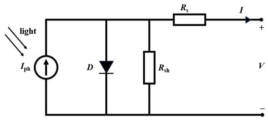
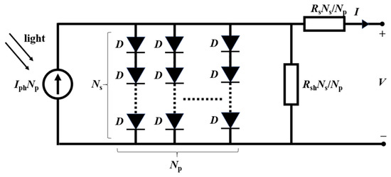
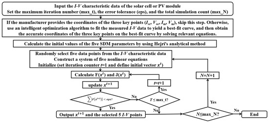
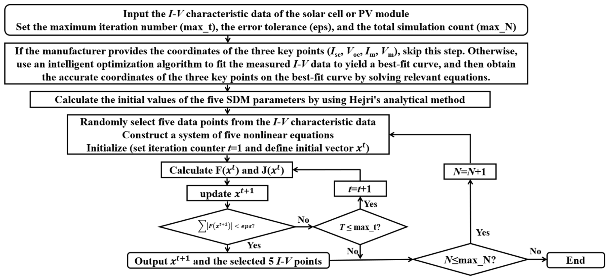
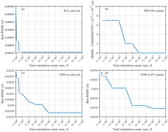
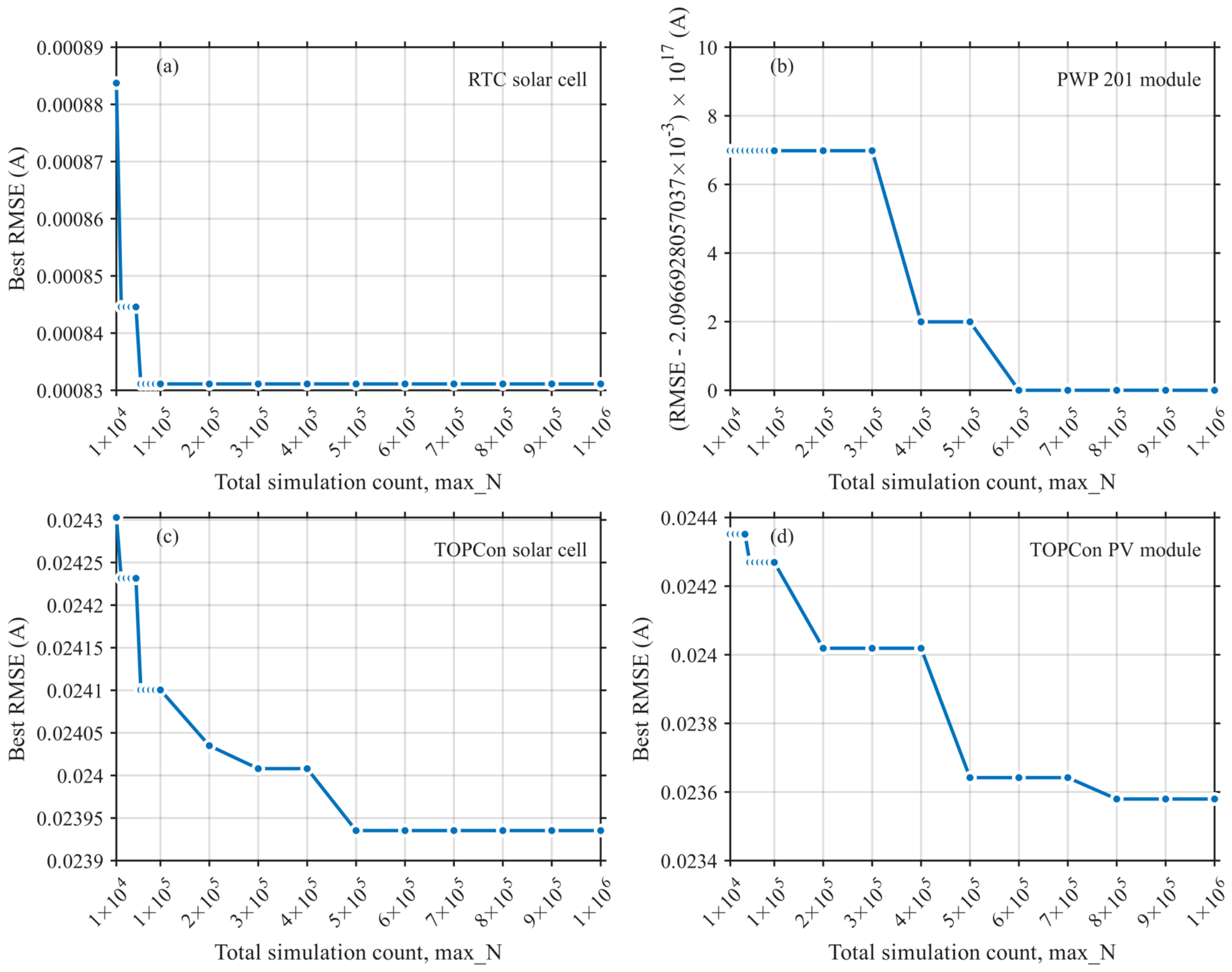
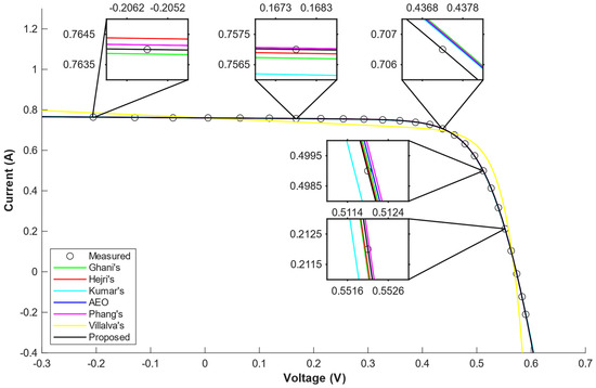
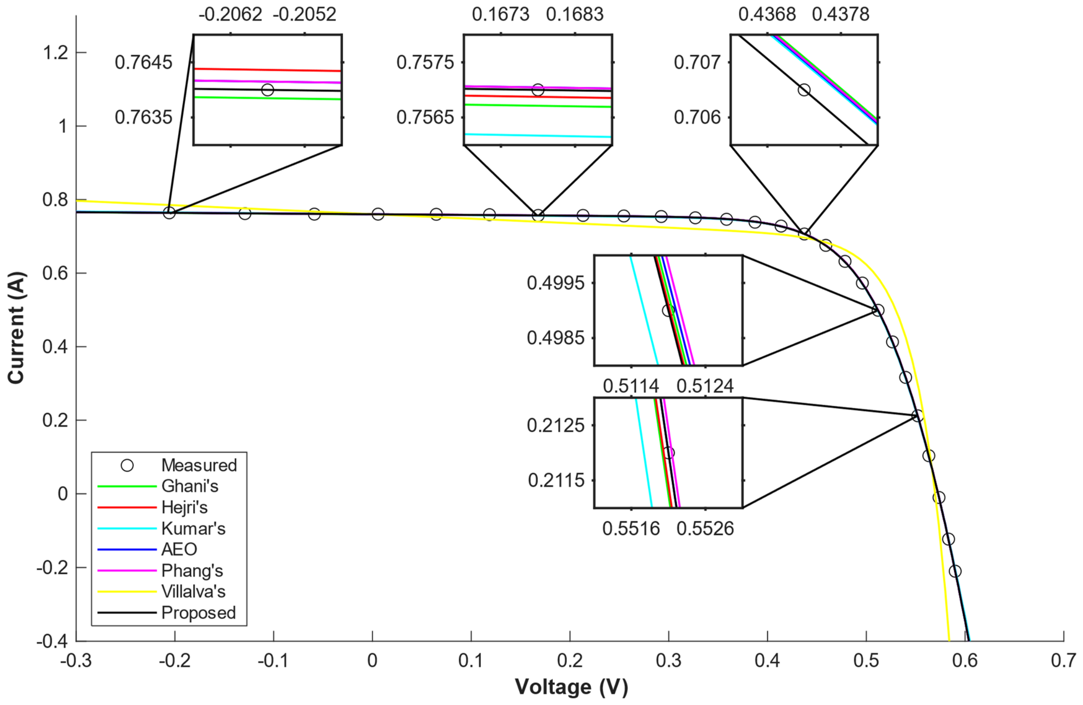
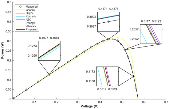
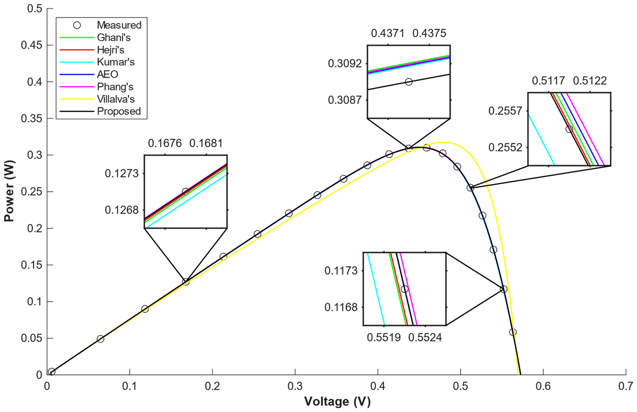
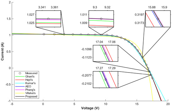
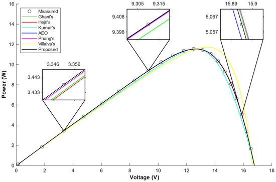
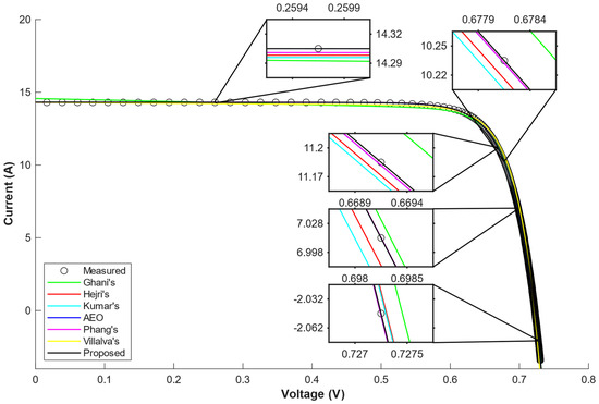
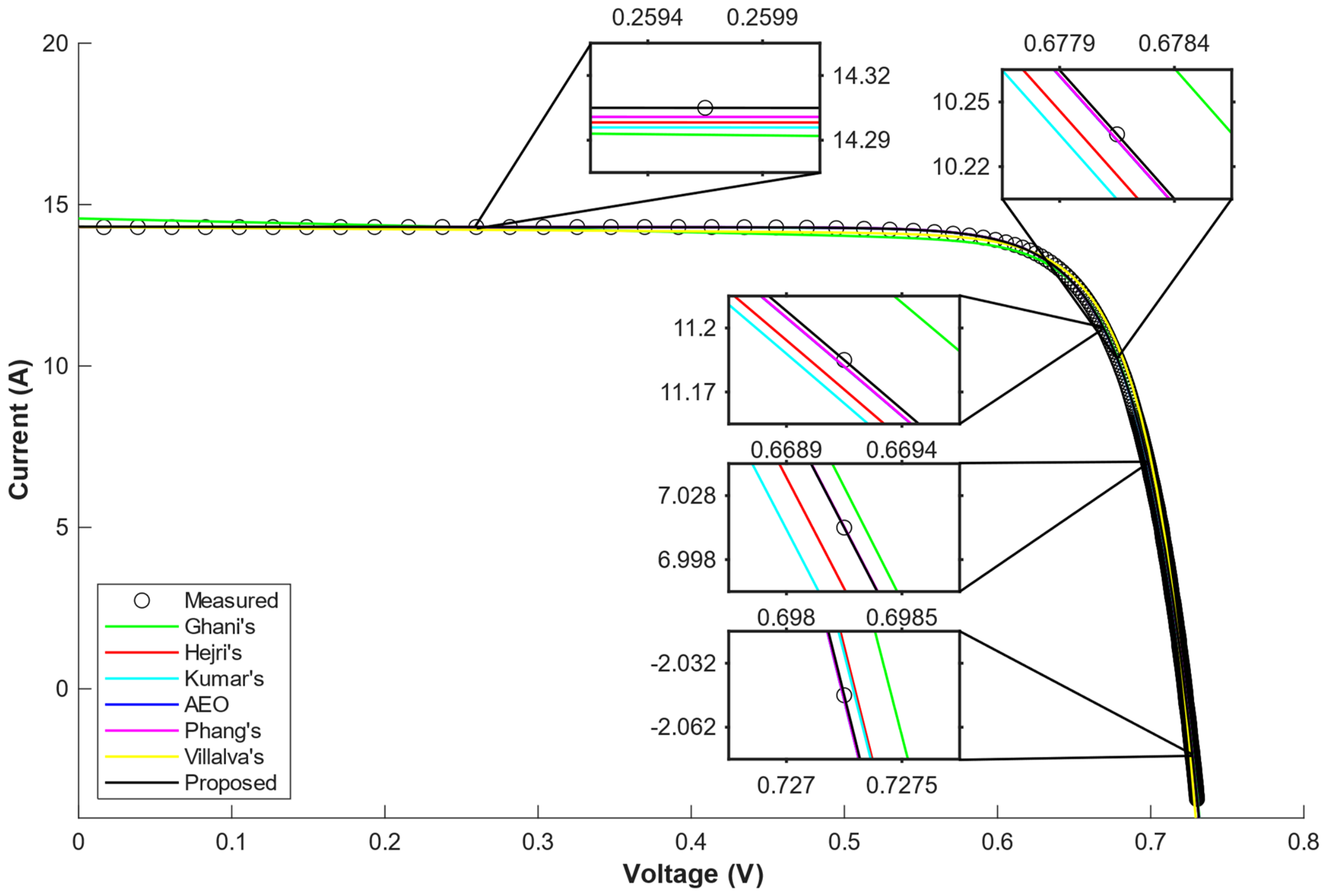
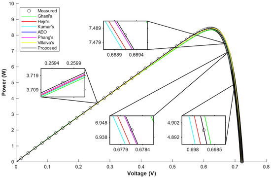
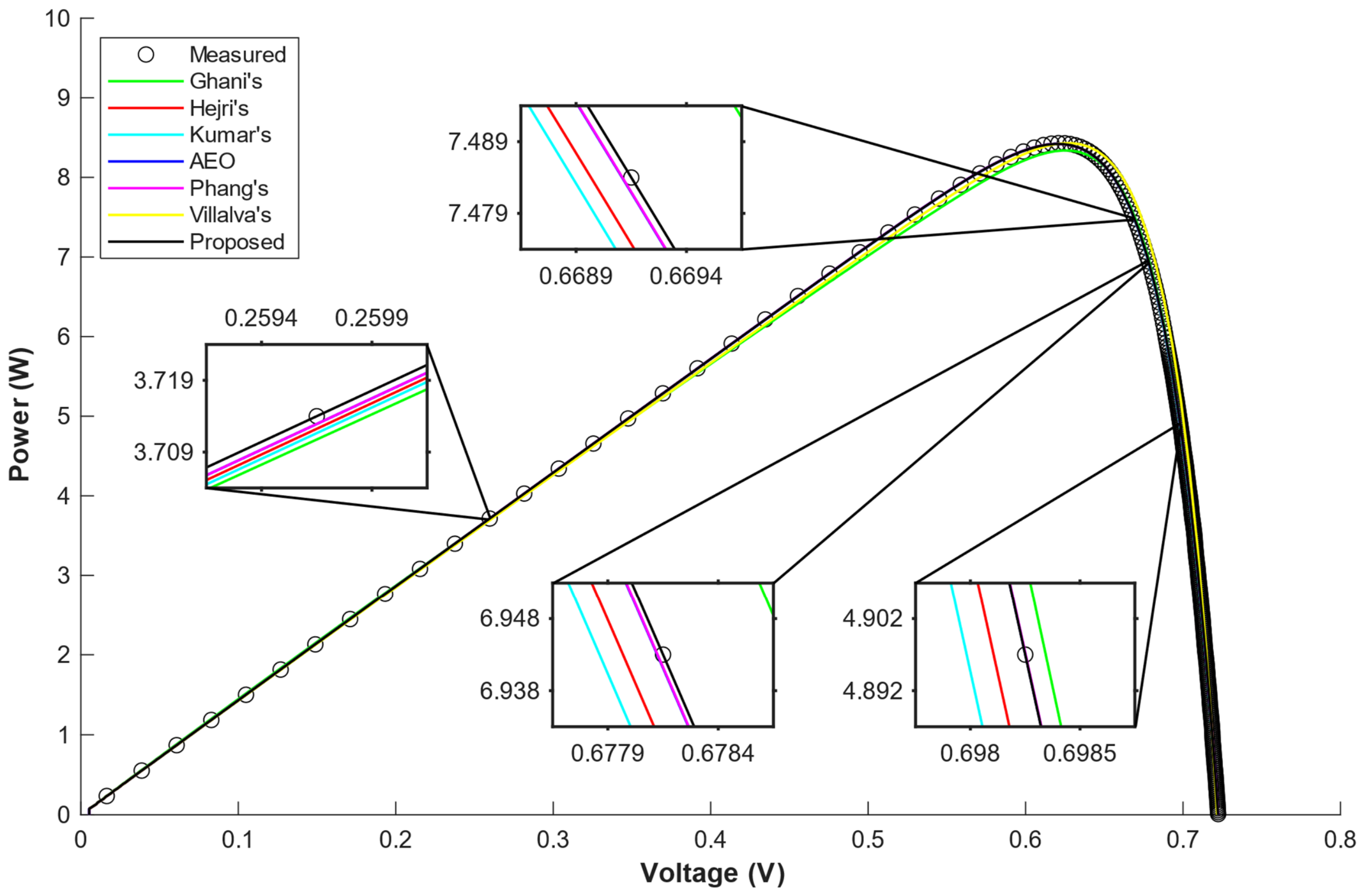
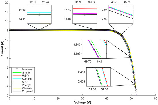
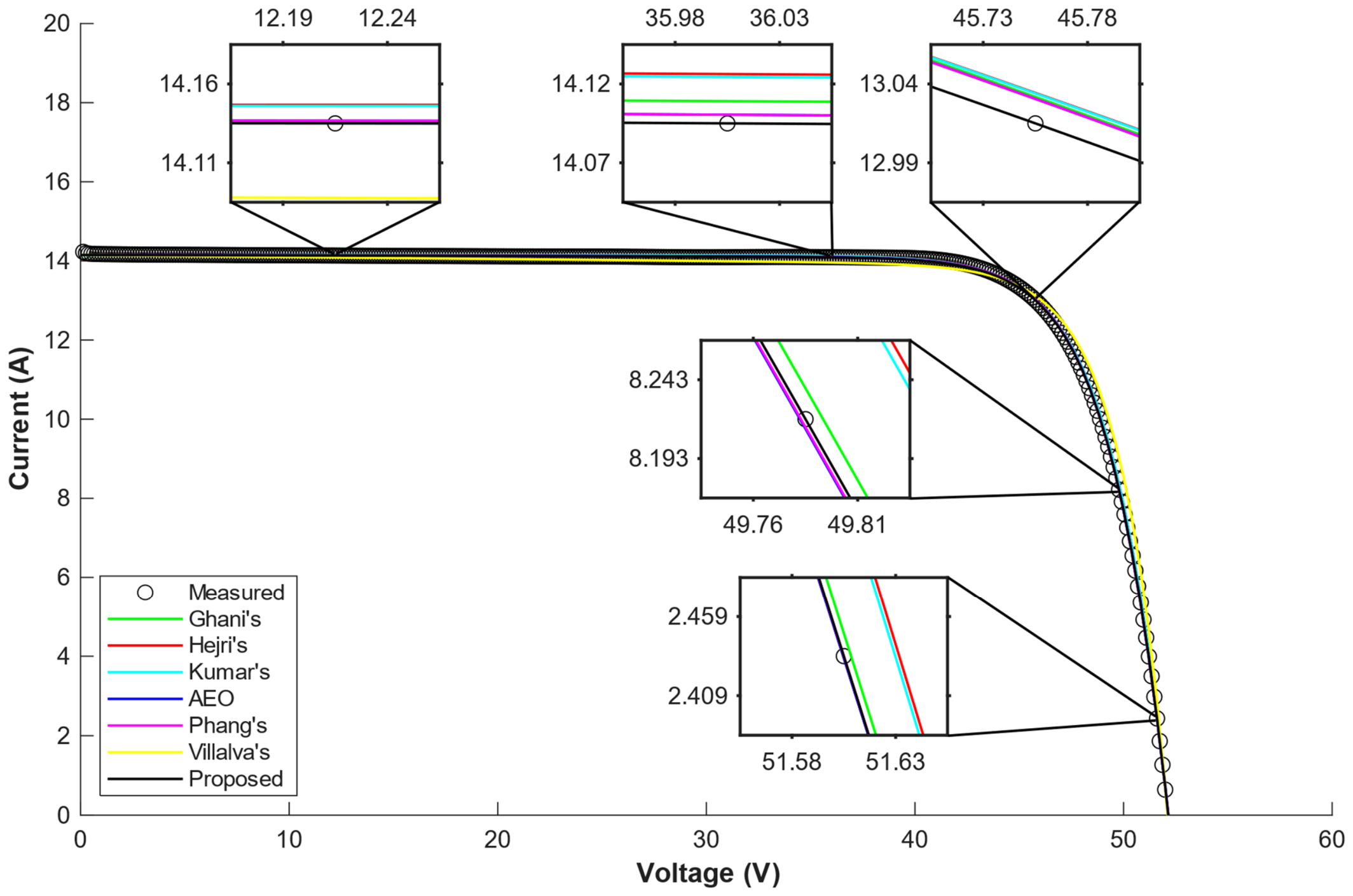
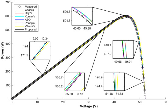
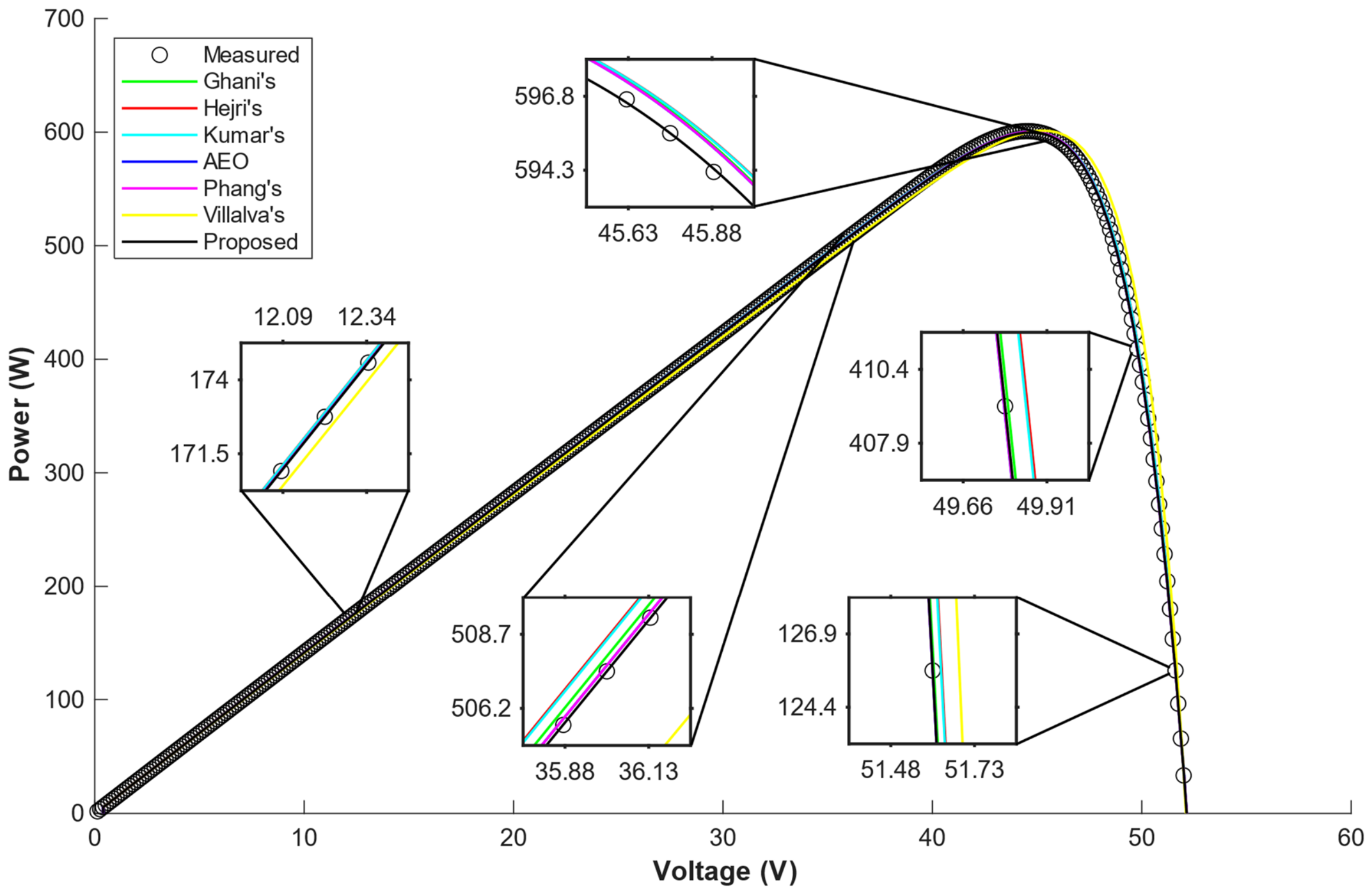

Disclaimer/Publisher’s Note: The statements, opinions and data contained in all publications are solely those of the individual author(s) and contributor(s) and not of MDPI and/or the editor(s). MDPI and/or the editor(s) disclaim responsibility for any injury to people or property resulting from any ideas, methods, instructions or products referred to in the content. |
© 2026 by the authors. Licensee MDPI, Basel, Switzerland. This article is an open access article distributed under the terms and conditions of the Creative Commons Attribution (CC BY) license.