


Abstract
Wind power ramp events (abrupt swings in output driven by frontal passages, sea-breeze transitions, and turbulence) are among the hardest problems for operators integrating renewables. Forecasting models are usually judged by aggregate error metrics (MAE, RMSE, overall directional accuracy) that average stable and ramp periods together, masking how a model behaves during the ramps that actually stress the grid. We address this on two fronts. First, we propose a regime-stratified evaluation that reports ramp event directional accuracy (ramp-DA) separately from stable-period accuracy and argue that ramp-DA should be a primary metric for grid-integration forecasting. Second, we build an ensemble of five regime-specialised sub-models trained with a direction-focused loss that penalises sign errors in the forecast power change, using only on-site SCADA wind speed and power. On 33,411 held-out samples from three onshore Greek farms, the ensemble reaches 76.5% ramp-DA, against 70.1% for a two-layer LSTM (+6.4 pp) and 74.3% and 74.1% for the PatchTST and iTransformer baselines. A strict leave-one-farm-out test retains 77.4% ramp-DA on a fully unseen farm. Overall directional accuracy rises 3.4 points, evidence that aggregate metrics understate the ramp-focused gain, while mean absolute error falls 19% compared to the LSTM (Diebold–Mariano p < 0.001).
1. Introduction
1.1. The Ramp Event Problem
Wind power has grown from a marginal contributor into a backbone of the global electricity system, and that growth has exposed a basic weakness in existing short-term forecasting: models that perform well on average can still fail systematically in the conditions of greatest operational consequence. Ramp events, intervals in which output changes by a large fraction of rated capacity within minutes, impose severe stress on transmission systems and force the rapid deployment of spinning reserves, sometimes load shedding, and coordination across several generation assets [1,2]. A single unforecast ramp can carry disproportionate balancing and reserve costs, and those costs grow as wind penetration rises [3,4].
Ramps are also meteorologically diverse. Drawing on the ramp causation literature, we group their drivers into five broad physical mechanisms—synoptic-scale frontal passages; mesoscale sea-breeze circulations; orographic gap-flow acceleration; sub-hourly turbulent gusts; and slow, multi-hour trends driven by approaching weather systems—each operating on its own spatial scale and predictability horizon [5,6]. This grouping is our own synthesis, rather than a taxonomy taken verbatim from any single source. The horizons differ sharply: a frontal ramp may be foreseeable several hours ahead from NWP pressure tendency fields, whereas a turbulent gust is essentially stochastic at 10 min resolution. Because no single architecture can capture this range of scales at once, we build one sub-model for each characteristic scale, described below.
Standard deep learning forecasting models compound this challenge by optimising mean squared error across all time steps equally. In a dataset where 46.1% of 10 min intervals are ramp events and 53.9% are stable, an MSE-minimising model will allocate most of its capacity to the stable majority, since correct stable-period predictions contribute more to the aggregate loss reduction. The result is a model that performs well on average but provides limited improvement over naive persistence precisely during the ramp events that destabilise the grid.
1.2. The Metric Problem
Standard practice in wind power forecasting reports overall MAE, RMSE, and directional accuracy averaged across every time step. This creates a mismatch between what the metrics measure and what actually governs operational decisions. Consider a hypothetical model that forecasts stable intervals perfectly (53.9% of our test set) but does no better than chance during ramp events (46.1%): its aggregate directional accuracy would be about 77%, an apparently strong figure that carries no operational value for the reserve-scheduling decisions ramp drive. A model designed the other way, sacrificing a little stable-period accuracy to capture ramp direction, would look mediocre on aggregate metrics, yet prove far more useful to grid operators.
This metric design problem is well documented through the literature. Bianco et al. (2016) observed that standard statistical metrics treat ramp events no differently from any other interval and built a dedicated ramp tool and metric to measure skill during ramps [7]. Ferreira et al. (2011) surveyed the gap between aggregate accuracy and ramp-specific performance across many methods [8], while Madsen et al. (2005) provided a standardised evaluation protocol and warned that the choice of error measure strongly shapes how models rank, so aggregate measures such as RMSE need not reflect performance on particular event types [9]. A 2025 critical review of data-driven wind and solar ramp methods finds the gap still open: detection algorithms have matured, yet existing approaches struggle with localised ramp phenomena, and the authors single out sample imbalance and ramp-specific metrics as unresolved [10]. We focus on this gap directly, proposing ramp event directional accuracy as the primary metric and supporting the choice with both a methodological argument and empirical evidence.
1.3. Contributions
This paper makes the following specific contributions:
- Regime-stratified evaluation framework decomposing DA into ramp-DA and stable-DA, demonstrating that aggregate metrics systematically understate operational value during the intervals that matter most for grid operators.
- Ensemble of five regime-specialised models trained with a direction-focused loss that explicitly penalises errors in the sign of the forecast power change, concentrating learning pressure on correct ramp direction.
- Empirical demonstration that the ensemble achieves 76.5% ramp-DA (95% CI 75.8–77.1; +6.4 pp vs. the LSTM and +2.2/+2.4 pp vs. the PatchTST/iTransformer baselines, all paired bootstrap-significant) while overall DA improves by only +3.4 pp, confirming that aggregate metrics understate the ramp-focused gain.
- Regime-adaptive prediction intervals (wider during ramps, narrower during stable periods) that provide informative, regime-sensitive uncertainty indicators. We show these spread-based intervals are not yet calibrated (test coverage 76.8% at the nominal 95% level) and should therefore be read as qualitative uncertainty signals.
2. Related Work
2.1. Wind Power Ramp Forecasting
Ramp forecasting has been studied as a distinct subproblem for over a decade, motivated by the recognition that standard forecast accuracy metrics do not adequately reflect performance during ramp events, which prompted the development of dedicated ramp-specific tools and metrics [7]. Physical NWP post-processing was the first approach [11]; statistical regime-switching models improved over persistence, but could not incorporate spatial meteorological drivers [12]. Cui et al. (2023) combined LSTM with a dynamic swinging-door algorithm for ramp detection, achieving meaningful day-ahead improvement over NWP baselines [3]. Graph attention networks incorporating spatial wind propagation between farms have shown promise for mesoscale ramp precursors on the Baidu KDD Cup 2022 and NREL WIND Toolkit datasets [13]. Regime-switching neural networks have improved short-term ramp event forecasting by adapting to distinct atmospheric states [14]. Feature extraction combined with CNN-LSTM on Belgian ELIA data has achieved annual average ramp recall of 0.9059 [15]. Oversampling methods addressing class imbalance (EB-LOS) have reached recall of 0.8196 on eight Chinese farms [16]. Finally, a stochastic scenario-generation method for ramp event forecasting has demonstrated strong probabilistic performance on data from a Bonneville Power Administration wind plant [17].
The Metric Landscape: Classification vs. Directional Accuracy
Most ramp forecasting studies pose the task as binary classification (ramp vs. no ramp) and report classification metrics: recall (the fraction of actual ramps detected), precision (the fraction of predicted ramps that occur), the Critical Success Index (CSI, which penalises both misses and false alarms), the F1 score, and the bias index [7,15,16]. Our formulation measures something different. Directional accuracy is the fraction of time steps at which the predicted direction of the power change (up, down, or none) matches the observed direction; ramp-DA restricts that fraction to intervals where the power change exceeds 0.05 p.u., and stable-DA covers the rest. This is the question reserve scheduling actually generates: not whether a ramp will occur, but whether output will rise or fall. A direct comparison between our ramp-DA (76.5%) and published recall figures (0.82–0.91) [15,16] would therefore be misleading, because the task definitions, datasets, and thresholds differ enough to make the numbers incommensurable.
2.2. Ensemble and Probabilistic Approaches
Probabilistic ensemble frameworks for offshore wind power fluctuations have been developed using Markov switching and scenario-based methods [18]. Minute-scale probabilistic prediction using dual-Doppler radar has demonstrated strong ramp detection performance for offshore turbines [19]. Our work complements these by embedding a direction-focused penalty directly in the training loss, targeting correct ramp direction, rather than probabilistic spread. A complementary, first-principles line of work uses physics-informed neural networks that embed the governing flow equations directly into the learning objective. For example, a PINN formulated on the non-dimensional Navier–Stokes equations have recently been shown to provide an effective means of evaluating wind turbine wake effects [20]. Such physics-informed formulations target the fluid dynamic structure of the flow field, whereas our approach is deliberately data-driven and operational, using only on-site SCADA wind speed and power signals. The two methodologies can be considered complementary, and coupling wake-resolving physics with regime-stratified operational evaluation is an interesting task for future work.
2.3. Positioning
To our knowledge, no prior study has (i) used ramp event directional accuracy as the primary metric in place of recall/CSI, or (ii) demonstrated empirically that aggregate DA and ramp-DA lead to qualitatively different conclusions about model value. The closest related work is the ordinal regression framework of Hu et al. (2023) [21], which distinguishes up-ramps, non-ramps, and down-ramps, a three-class formulation conceptually aligned with our directional framing, but reports standard classification metrics, rather than stepwise directional accuracy, and does not stratify results by ramp regime. Our work provides validated empirical results on real SCADA data under a clearly defined metric that directly corresponds to the reserve-scheduling decision, with full statistical testing (DM p < 0.001, bootstrap CIs).
Recent advances in multivariate time-series forecasting have introduced highly effective transformer architectures, notably PatchTST [22] and iTransformer [23]. We implemented appropriately sized versions of both (channel-independent patching with instance normalisation for PatchTST, inverted variate-token attention for iTransformer, approximately 0.4 M parameters each) and trained them under the identical protocol applied to our other deep baselines (AdamW, up to 300 epochs with early stopping, batch 64, MSE objective, 48-step lookback). The models have been evaluated on the same held-out test set and regime split (Section 6.1), and the transformers were the strongest point-forecast baselines, matching the ensemble on mean absolute error, yet the ensemble retains a statistically significant advantage on the operationally decisive directional metrics (paired bootstrap ramp-DA gains of +2.2 pp over PatchTST and +2.4 pp over iTransformer, both 95% CIs excluding zero). This is consistent with our central thesis: the contribution of this work is the regime-stratified evaluation metric (ramp-DA) and the direction-focused training protocol, which are orthogonal to, and composable with, the choice of underlying regressor. Integrating a transformer as an additional specialist within the ensemble is a natural extension we identify as future work.
3. Datasets
3.1. Sources
Our experiments are based on three onshore wind farms in the Peloponnese, Greece (TERNA Energy, January 2017–May 2018), representing coastal sea-breeze, inland thermal, and orographic channelling regimes. SCADA wind speed and active power at 10 min intervals are the sole input signals; all predictive features are engineered from these two on-site measurement streams (Section 3.3). Quality control (duplicate-timestamp removal, alignment to a common 10 min grid, time-based interpolation of gaps, and clipping of physically invalid negatives) retained 98.7% of raw timesteps. The data were split chronologically into 70% train, 15% validation, and 15% test, providing a test set of 33,411 samples spanning approximately six calendar months.
Because the three farms are concatenated before the chronological split, the training set comprises two of the farms (denoted Farm A and Farm B) in full, together with only the earliest 10% of the third (Farm C); 95.2% of training samples come from the two non-evaluation farms, while the validation and test sets fall entirely within the later, unseen 90% of Farm C. The reported metrics therefore reflect predominantly cross-site transfer: the ensemble is trained almost entirely on two regionally distinct farms and evaluated on a third whose evaluation period was not seen in training. To remove even the 4.8% residual overlap, we additionally report a strict leave-one-farm-out experiment in Section 6.8, in which the models are trained exclusively on Farms A and B and evaluated on the entirety of Farm C; that experiment confirms strong absolute transfer to a fully unseen site, while scoping the ensemble’s advantage over the recurrent baseline to the within-region setting. To respect data confidentiality obligations, the three sites are referred to only as Farms A–C, and their precise locations are withheld.
3.2. Ramp Event Definition
Ramp event: |Δpower(t)| = |P(t) − P(t−1)| > 0.05 p.u. per 10 min step, following the threshold-based power change definition adopted by Ferreira et al. (2011) [8] and the ramp-identification approach of Bianco et al. (2016) [7]. Prevalence in test set: 46.1% of intervals (15,396 of 33,411 samples). This high prevalence reflects the strongly diurnal wind resource of the Peloponnese sites, where thermal and sea-breeze cycles drive frequent power changes.
In operational terms, 0.05 p.u. is a change of 5% of rated capacity within a single 10 min settlement interval, equivalent to a sustained ramp rate of about 0.3 p.u. per hour (30% of rated capacity per hour). It is the smallest single-step change that carries operational weight for intra-hour balancing at these sites: smaller changes sit within the noise band of normal turbine operation, whereas changes at or above the threshold are large enough to require an adjustment of committed reserves within the same or the following dispatch interval. The threshold is therefore deliberately permissive by the standards of the ramp literature, where amplitude thresholds typically span 10–75% of installed capacity over windows of five minutes to six hours. By design, it isolates the short, frequent, sub-hourly fluctuations most relevant to real-time reserve deployment, rather than the larger multi-hour ramps emphasised in day-ahead unit-commitment studies. This choice is the main reason the measured prevalence is high, and it makes that prevalence strongly threshold-dependent and not directly comparable to studies using larger thresholds or longer windows. We match the single-step threshold to the 10 min horizon at which the model operates and leave the longer accumulation windows to future work as a complementary evaluation.
A threshold sensitivity analysis (Table 1) confirms that the ensemble’s directional advantage does not depend on this choice. As the threshold tightens from 0.05 to 0.25 p.u., prevalence falls from 46.1% to 10.7%, while ensemble ramp-DA rises monotonically from 76.5% to 91.3%, and the LSTM from 70.1% to 83.3%. The ensemble holds a consistent +6.4 to +8.5 pp advantage at every threshold, and the margin widens for the larger, grid-critical ramps, so the reported gains are not artefacts of the permissive 0.05 p.u. definition.
Table 1.
Ramp threshold sensitivity (held-out test set, n = 33,411). As the |Δpower| threshold is tightened, prevalence falls and directional accuracy rises for both models.
3.3. Input Features
The model uses a 20-feature representation, all engineered from the two on-site SCADA signals (wind speed and active power). (i) Raw signals: normalised wind speed and normalised active power (the prediction target). (ii) Lags: wind speed and active power lags at 1, 6, 12 and 48 steps (10 min to 8 h). (iii) Rolling statistics: 1 h and 8 h rolling means of wind speed and the 1 h rolling standard deviation of wind speed. (iv) SCADA-derived dynamics: the first difference in active power (a ramp indicator), a wind speed variability ratio (rolling standard deviation divided by rolling mean), and wind speed cubed (proportional to the kinetic energy of the flow). (v) Temporal: sine/cosine encodings of hour-of-day and month-of-year. All twenty features are derived exclusively from the two on-site SCADA streams and the specialist names used later (e.g., wide-context, multi-scale) denote the ramp regimes each model is tuned to capture, not external meteorological inputs. All features were scaled to [0, 1] using a min–max scaler fitted on the training split only, to avoid information leakage.
4. Methodology
4.1. Architecture Overview
The proposed forecasting system follows a mixture-of-experts design: five specialist sub-models, each configured to capture a distinct class of ramp dynamics, produce independent 10 min ahead power change predictions that are combined into a single ensemble forecast. Specifically, the five sub-models, (a) the short-window, (b) multi-scale, (c) diurnal-scale, (d) wide-context, and (e) slow-trend specialists, differ in their lookback window and architecture (Table 2), so that together, they cover the range of temporal scales over which ramps develop at these sites, from sub-hourly fluctuations to slow, multi-hour trends (Section 1.1). Because the model receives only on-site SCADA wind speed and power, each sub-model was defined by its configuration; hence, the number of the sub-models have not been investigated, as the primary target was the aforementioned temporal scales.
Table 2.
Specialist sub-model architectures and ramp event directional accuracy on the held-out test set. Ensemble outperforms all individual specialists on ramp-DA (76.5%) while achieving the second-lowest MAE (0.089).
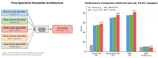
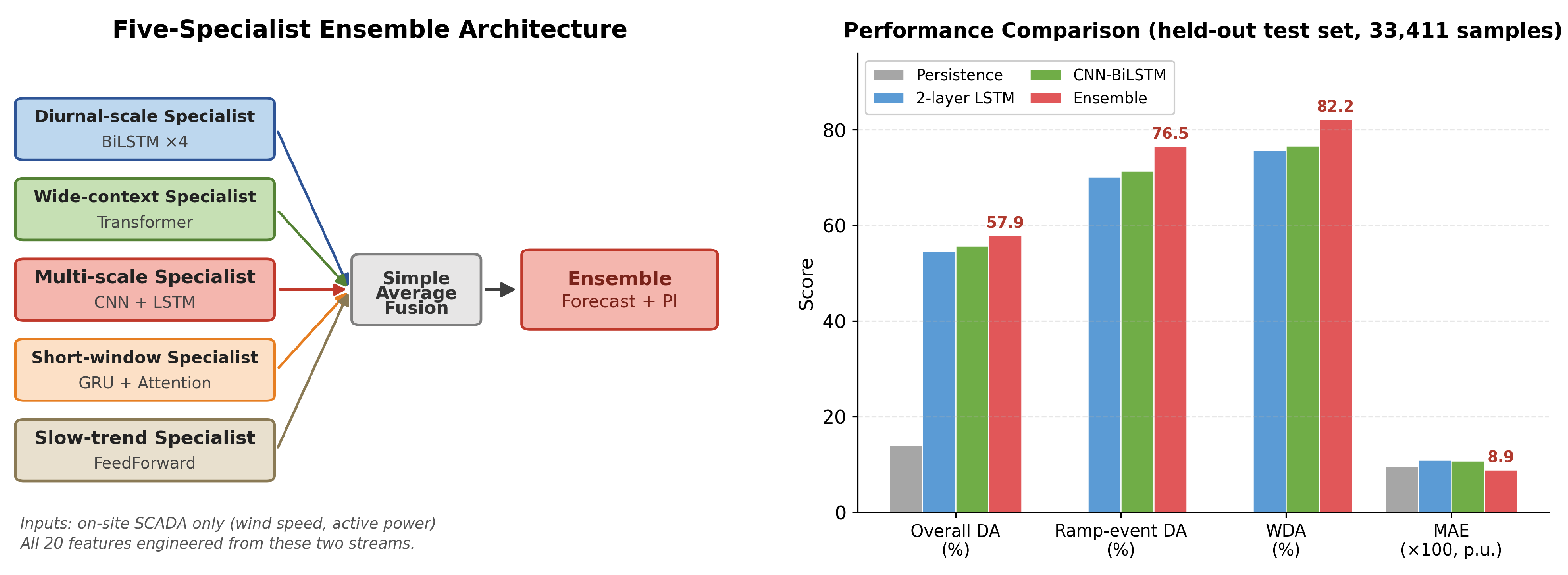
The five sub-models’ outputs are combined by simple averaging, where we evaluated learned gating on the validation set and found no appreciable improvement over simple averaging, while gating introduced substantial training complexity and instability. This is consistent with the broader forecast combination literature, in which simple fixed-weight averaging is often competitive with more complex learned combination schemes, particularly when the constituent models are sufficiently diverse in their error patterns. Concretely, the sub-models’ continuous power change predictions are averaged and the sign of the averaged prediction defines the ensemble direction. Averaging decorrelated specialist errors reduces prediction variance, which is the mechanism by which the ensemble can marginally exceed the best individual sub-model on ramp-DA. Figure 1 illustrates the full architecture and the performance comparison against baselines on the held-out test set.
Figure 1.
Ensemble architecture and performance summary. (Left) five-specialist mixture-of-experts design with simple average fusion. (Right) performance comparison across all models on the held-out test set (33,411 samples). The ramp event DA column (second from left) shows the primary contribution: a +6.4 pp ramp-DA improvement over the LSTM baseline. The ensemble’s forecast error advantage over the LSTM is statistically significant by a Diebold–Mariano test on the absolute-error differential of the 10 min series.
4.2. Specialist Sub-Models
Table 2 summarises specialist architectures, target regimes, and held-out test performance. Ramp-DA ranges from 67.2% (wide-context) to 76.1% (multi-scale). The short window sub-model’s domain-filtered niche evaluation of the 217 highest-turbulence test samples yields a result below the 50% random-direction baseline; consistent with the fundamental stochasticity of turbulence at 10 min resolution, this niche DA is excluded from primary results and addressed in Section 7.2. We caution that 217 samples is a small subset for which the directional accuracy estimate carries a wide confidence interval (of the order of ±7 pp at this sample size). Finally, the sub-50% value should therefore be interpreted as statistically indistinguishable from chance, rather than as evidence of systematically wrong-signed prediction, which is consistent with the interpretation that turbulence is effectively unpredictable at this resolution.
4.3. Multi-Objective Direction-Focused Loss
Each specialist is trained with a multi-objective loss that combines forecast accuracy with an explicit penalty on directional error:
is the mean squared error between the predicted and observed power at the forecast step, anchoring the magnitude of the forecast. is the directional term and is the key design choice: it is a margin-based penalty on the agreement between the predicted and the observed direction of the power change. The predicted change and the observed change are each taken relative to the last observed value and penalises the model whenever these two changes fail to agree in sign by at least a fixed margin, so that predictions whose directions disagree with the observed movement incur a loss, while confident, correctly signed predictions are rewarded. This concentrates learning pressure on correctly obtaining the direction of the next power change correct. is a margin-based penalty between the predicted and observed power change, and each ramp interval enters this term through the same fixed margin. Magnitude information is used elsewhere in the framework, specifically in the mean-squared term L_mag, which anchors the forecast magnitude, and in the weighted directional accuracy (WDA) reported for evaluation, which up-weights intervals with larger power changes. Moreover, is a temporal smoothness penalty on the first difference in successive predicted steps, discouraging physically implausible step-to-step oscillation in the forecast trajectory.
The three weights (α, β, γ) were tuned per specialist by grid search on the validation set, allowing each regime model to balance magnitude, direction, and smoothness according to the dynamics it targets; the per-specialist values are reported in the supplementary configuration. A sensitivity analysis of performance to these weights and a comparison against adaptive multi-objective weighting schemes are noted as future work.
4.4. Uncertainty Quantification
Prediction intervals are formed as the ensemble mean plus or minus a calibrated multiple ζ of the ensemble spread σ_ens(t). The multiplier ζ is calibrated on the validation set to achieve nominal 95% coverage (PICP). We deliberately avoid the term ‘conformal’: these intervals are not constructed by a split- or full-conformal calibration procedure and therefore carry no finite-sample coverage guarantee; genuine conformal calibration is discussed as an extension in Section 7.2 [24]. Because the width scales with σ_ens(t), the intervals are regime-adaptive, wider when specialists disagree (ramp events) and narrower when they agree (stable periods).
5. Implementation Details
PyTorch 1.12.1, NVIDIA A100 (Google Colab Pro). Two-stage training: (i) specialist pre-training, 1000 epochs, AdamW, per-specialist lr (diurnal-scale 0.000589, wide-context 0.000104, multi-scale 0.00329, short-window 0.000540, slow-trend 0.000303), grad clip 1.0, early stopping patience = 80 on validation DA; (ii) PI calibration of validation set. Sequence lengths: diurnal-scale 48 steps, wide-context 48, multi-scale 36, short-window 12, slow-trend 72. Batch size 64. Total: ~18 GPU-hours. All model code, training pipeline, and figure generation scripts are publicly available at https://github.com/Scientifico32/Ramp-Event-Forecasting (accessed on 4 July 2026).
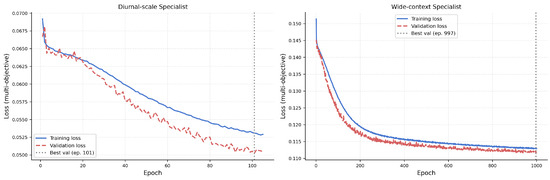
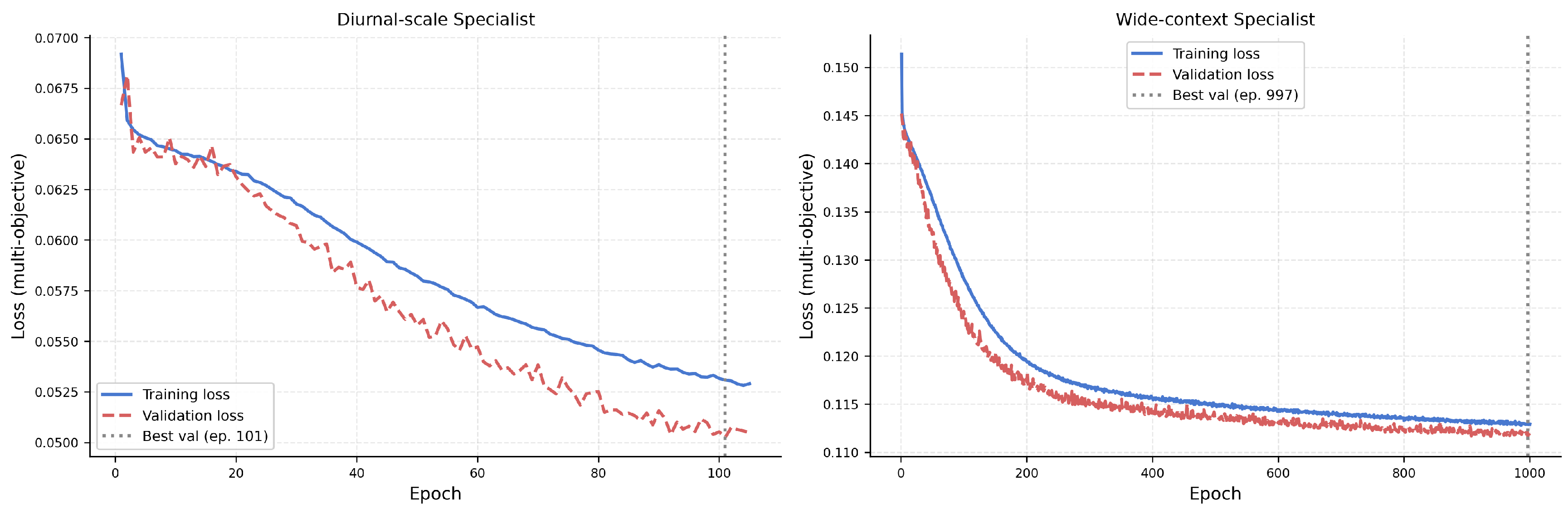
Figure 2 shows training and validation loss curves for the diurnal-scale and wide-context sub-models, confirming smooth convergence without overfitting. A loss-component ablation centred on ramp-DA and retrained across three random seeds (detailed in Section 6.6) shows that ramp-DA, stable-DA, WDA and overall DA all vary by less than the run-to-run standard deviation across the three loss settings (MSE only; MSE + direction; MSE + direction + temporal).
Figure 2.
Training and validation loss curves for the diurnal-scale (left) and wide-context (right) sub-models.
A turning point occurs at timestep t when sign(Δpower(t)) ≠ sign(Δpower(t − 1)) i.e., the power trajectory reverses from ascending to descending or vice versa, marking the peak or trough of a power excursion. Turning point accuracy (TPA) measures the fraction of actual turning points for which the forecast also changes sign within ±1 step (one-step tolerance to account for 10 min discretisation). Turning points are a subset of ramp events and represent the highest-consequence moments for reserve scheduling: the instant a ramp reverses is when the optimal reserve action changes.
6. Results
6.1. Primary Result: Ramp Event Directional Accuracy
Table 3 presents the full evaluation, where the primary result is the ramp-DA column: the ensemble achieves 76.5% versus 0.0% for persistence and 70.1% for the LSTM (+6.4 pp, DM p < 0.001; ensemble ramp-DA 95% CI [75.8, 77.1]%). The CNN-BiLSTM achieves 71.4%, so the specialist ensemble provides a further +5.1 pp over this single-architecture baseline. In addition, two transformer baselines, PatchTST [22] and iTransformer [23], were trained under the identical protocol and achieve 74.3% and 74.1% ramp-DA respectively. A paired bootstrap test on the ramp-DA difference (Table 4) confirms that the ensemble’s advantage over PatchTST (+2.2 pp, 95% CI [+1.5, +2.8]) and iTransformer (+2.4 pp, 95% CI [+1.8, +3.0]) is statistically significant, as it performed better than the LSTM (+6.4 pp) and CNN-BiLSTM (+5.1 pp). On squared-error accuracy, a Diebold–Mariano test finds the ensemble statistically indistinguishable from PatchTST (p = 0.42) and modestly superior to iTransformer (p = 0.015), so the ensemble’s decisive edge is specifically on the directional metrics that matter operationally, rather than on aggregate point error. The multi-scale sub-model achieves 76.1% ramp-DA individually, only 0.4 pp below the full ensemble. The ensemble’s advantage over the multi-scale specialist alone therefore lies in robustness: the ensemble is more robust than any single specialist, maintaining high ramp-DA, while individual specialists degrade on regimes outside their target regime. The Diebold–Mariano statistics are computed on the absolute-error differential. Because the held-out samples form a single contiguous chronological block from one farm, they are strongly serially dependent, so the effective sample size is smaller than the nominal count. The reported p-values and confidence intervals should therefore be read as indicative of a robust and consistent gain, rather than as exact significance levels. All confidence intervals reported here and in Table 3, Table 4, Table 5 and Table 6 were calculated under a seeded percentile bootstrap (500 samples) so that every model is treated identically.
Table 3.
Full performance metrics for the test set (33,411 samples). Bold indicates the proposed ensemble.
Table 4.
Paired percentile bootstrap differences.
Table 5.
Loss-component ablation centred on ramp-DA, mean ± standard deviation over three seeds (held-out test set; 15,396 ramp events). Directional metrics are flat to within the standard deviation; only MAE moves systematically, being lowest under MSE only.
Table 6.
Models trained on Farms A and B and evaluated on the entirety of the unseen Farm C.
In Table 4, every 95% interval excludes zero, so the ensemble’s advantage on both overall DA and ramp-DA is statistically significant against all four baselines. For reference, the Diebold–Mariano test on squared error gives ensemble vs. PatchTST p = 0.42 (n.s.) and ensemble vs. iTransformer p = 0.015, confirming the ensemble’s decisive edge is directional, rather than in point error.
6.2. Why Overall DA Is Not the Right Metric
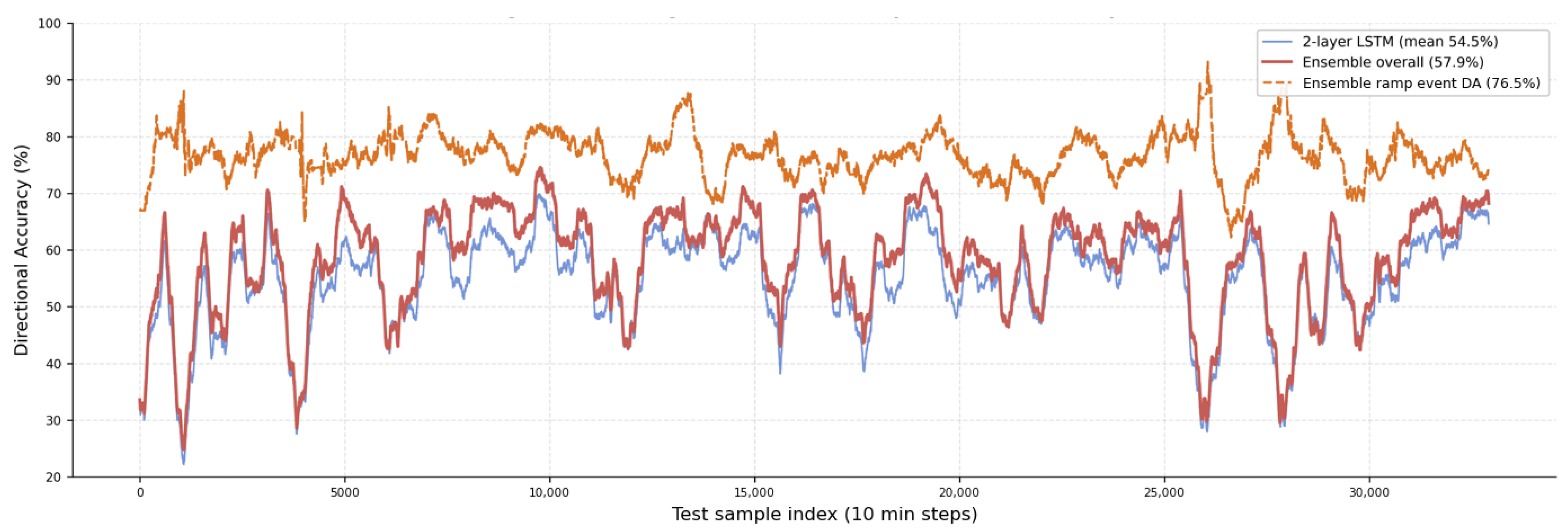
The ensemble reaches 57.9% overall DA, just +3.4 pp above the LSTM (54.5%), and that modest margin is by design. Stable intervals make up 53.9% of the test set, and every model handles them about equally (41.3–42.3%, a spread of one point), so an aggregate metric dominated by those intervals cannot separate the models by much. Because the regime-stratified design concentrates modelling capacity on ramp intervals, the ensemble’s real gain shows up in the weighted DA, which rises to 82.2% against the LSTM’s 75.6% (+6.6 pp) and concentrates the improvement on the large-|Δpower| intervals. Figure 3 makes the same point over time: across the six-month test period, the ramp event DA curve (orange dashed) sits clearly above overall DA throughout.
Figure 3.
Rolling directional accuracy over the test set (window = 500 steps ≈ 3.5 days). The ensemble ramp event DA (orange dashed, mean 76.5%) is consistently and substantially elevated above the overall ensemble DA (red solid, mean 57.9%) and the LSTM (blue, mean 54.5%), confirming that the regime-stratified advantage is stable across all seasons and weather patterns in the test period.
6.3. Magnitude Accuracy and Scatter
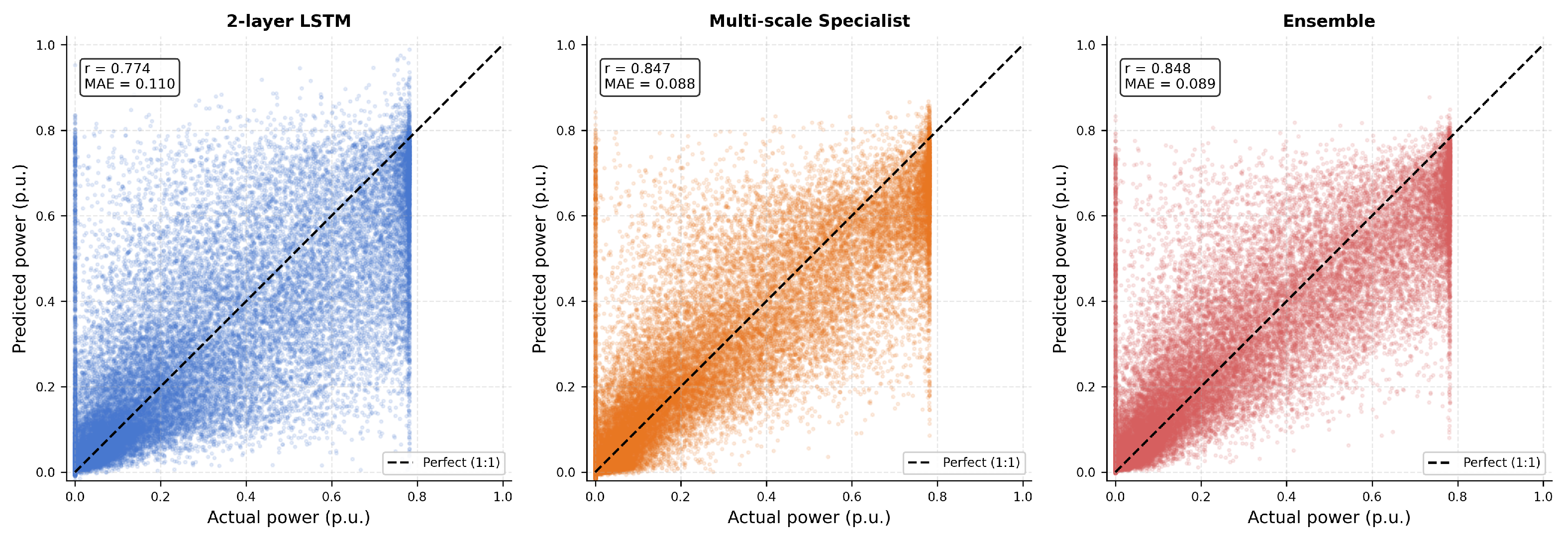
Figure 4 shows predicted vs. actual scatter plots for the LSTM baseline, the multi-scale sub-model (best individual model), and the ensemble. MAE = 0.089 p.u. (−19.1% vs. LSTM, DM p < 0.001). The multi-scale sub-model achieves MAE = 0.088 (marginally better than the ensemble), reflecting that ensemble averaging introduces slight magnitude smoothing in exchange for more robust ramp-DA across all regimes.
Figure 4.
Predicted vs. actual wind power scatter plots (normalised, p.u.) for the 2-layer LSTM baseline (left, r = 0.774, MAE = 0.110), the multi-scale sub-model (centre, r = 0.847, MAE = 0.088), and the ensemble (right, r = 0.848, MAE = 0.089). Dispersion decreases systematically from LSTM to ensemble, particularly at intermediate power levels (0.2–0.6 p.u.) corresponding to ramp event transitions.
6.4. 24-Hour Forecast Example
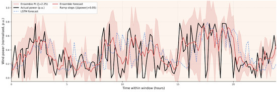
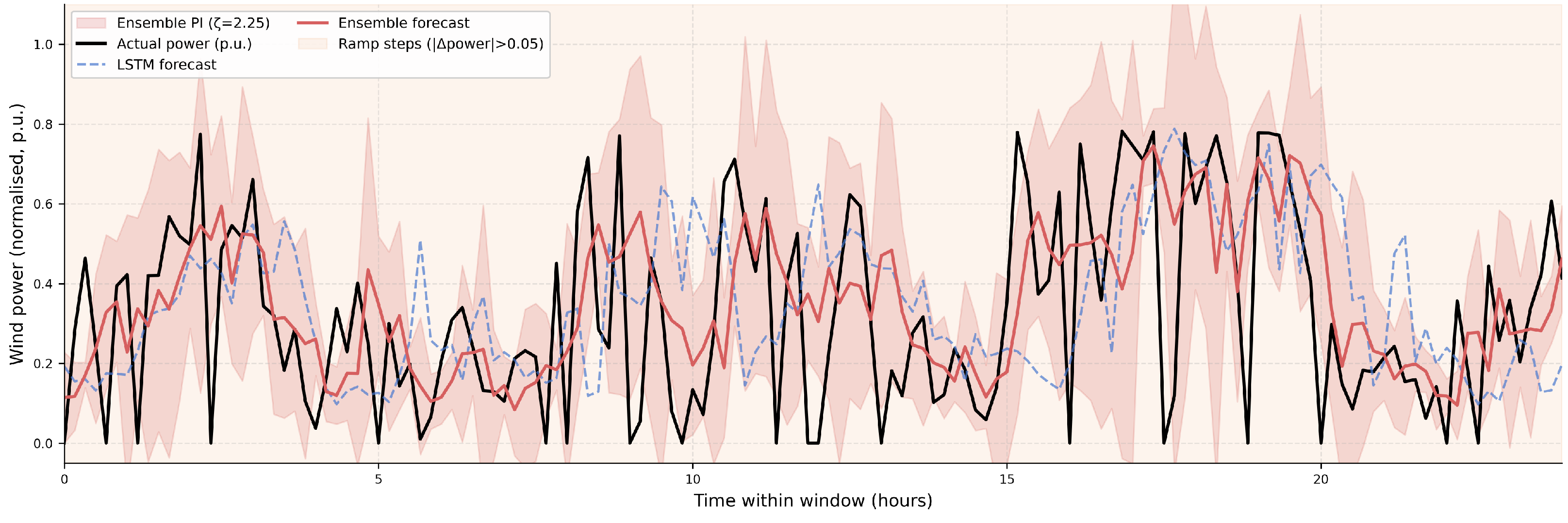
Figure 5 presents a representative forecast window from the held-out test set, deliberately selected for its high density of ramp events to illustrate model behaviour under the conditions that matter most operationally. The actual power (black) exhibits the frequent, large-amplitude swings characteristic of this strongly diurnal site. The ensemble forecast (red) tracks the broad trajectory of these transitions, capturing the directions of successive ramps, while the LSTM (blue dashed) follows the same general pattern, but with larger excursions during the most rapid changes, visually consistent with its lower ramp-DA (70.1% vs. 76.5%). Critically, the prediction interval (pink) is not of fixed width: it widens during periods of high ensemble disagreement and narrows when the specialists concur, realising the regime-adaptive uncertainty quantification described in Section 4.4. This behaviour is the operationally desirable one, as the model communicates elevated uncertainty precisely during the volatile, hard-to-forecast intervals when reserve-scheduling decisions carry the greatest risk, rather than reporting a single uninformative confidence level across all conditions.
Figure 5.
Forecast example over a ramp-dense window from the held-out test set. Black: actual power; red: ensemble forecast; blue dashed: LSTM; pink band: ensemble prediction interval (ζ = 2.25). The interval widens during high-disagreement periods.
6.5. Turning Point Detection
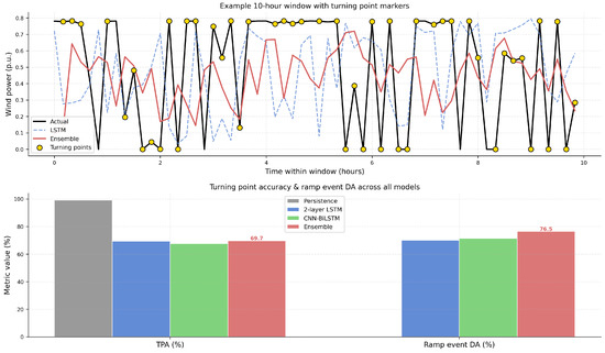
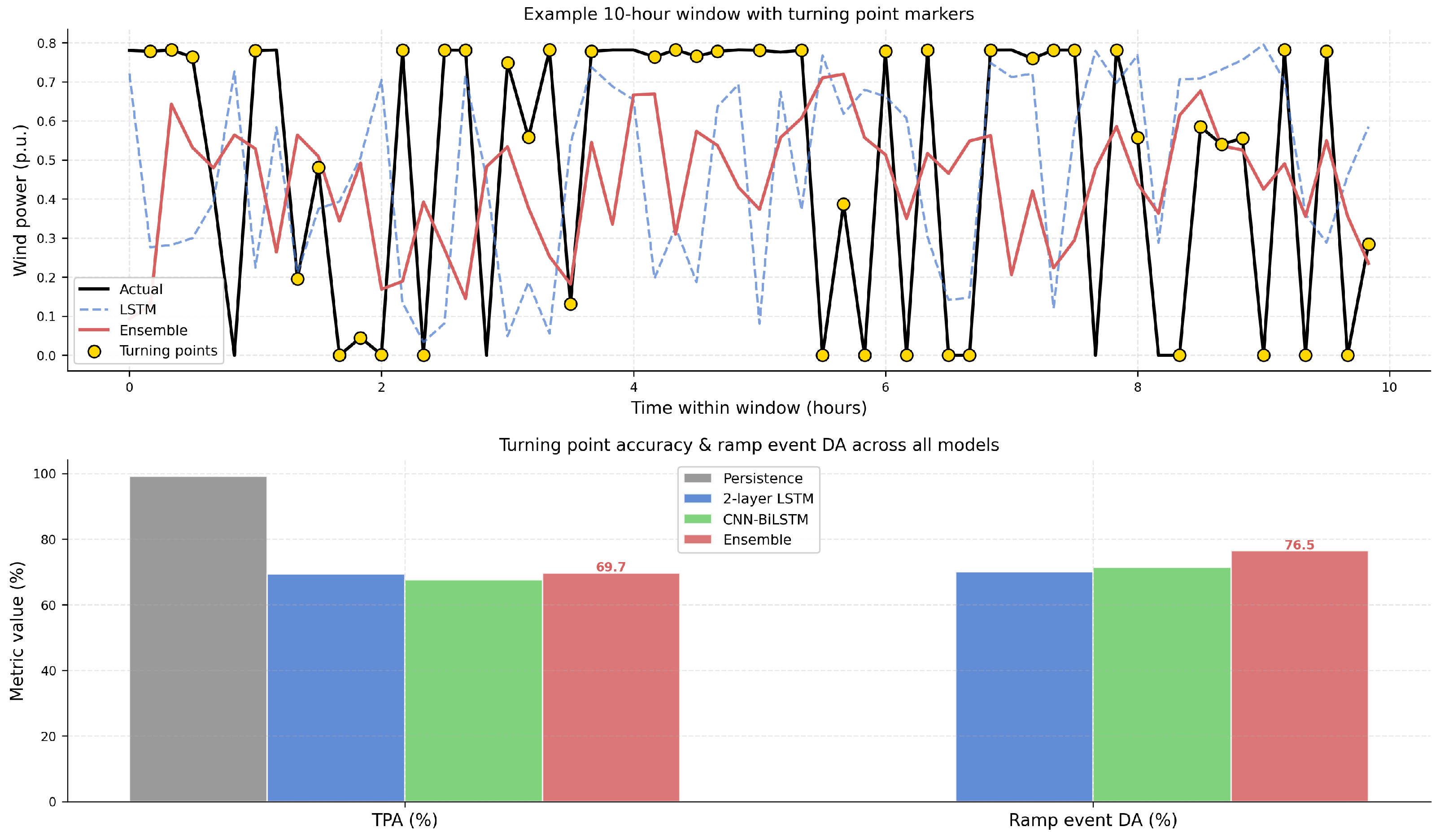
Figure 6 shows turning point detection of an example 10 h window. The ensemble achieves TPA = 69.7%, marginally above the LSTM (69.3%, +0.4 pp) and CNN-BiLSTM (67.7%). Persistence TPA is 99.2%, an artefact of the definition: persistence always predicts no change, so any stable-to-change transition trivially counts as a “detected” turning point, inflating the metric. Its ramp-DA of 0.0% confirms this high TPA carries no operational value. The bar chart (lower panel) reports TPA and ramp event DA across all models; on the operationally meaningful ramp-DA metric, the ensemble (76.5%) leads all models.
Figure 6.
Turning point detection performance. Upper: example 10 h test window with actual turning point markers (gold), ensemble forecast (red), and LSTM forecast (blue dashed). Lower: TPA and ramp event DA across all models. Persistence TPA = 99.2% is a definitional artefact (see Section 7.2); its ramp-DA = 0.0% confirms operational worthlessness during ramp events.
6.6. Architecture Ablation
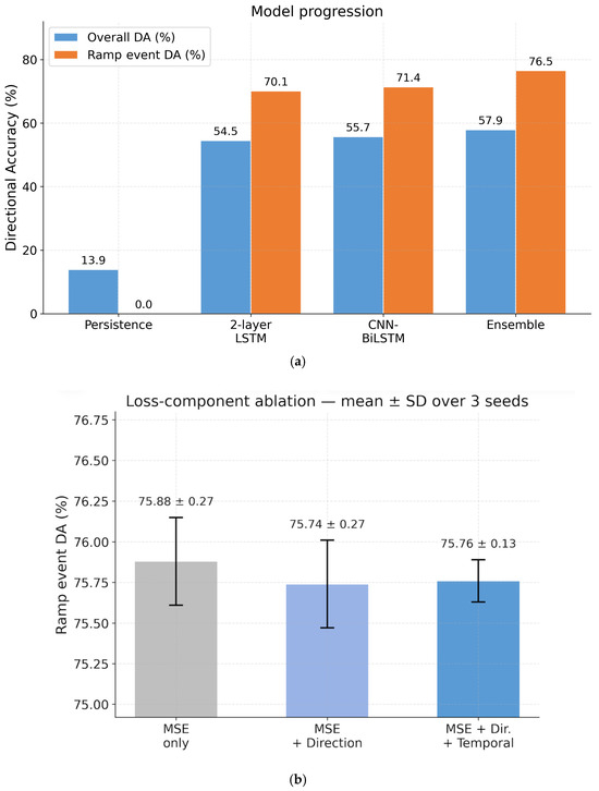
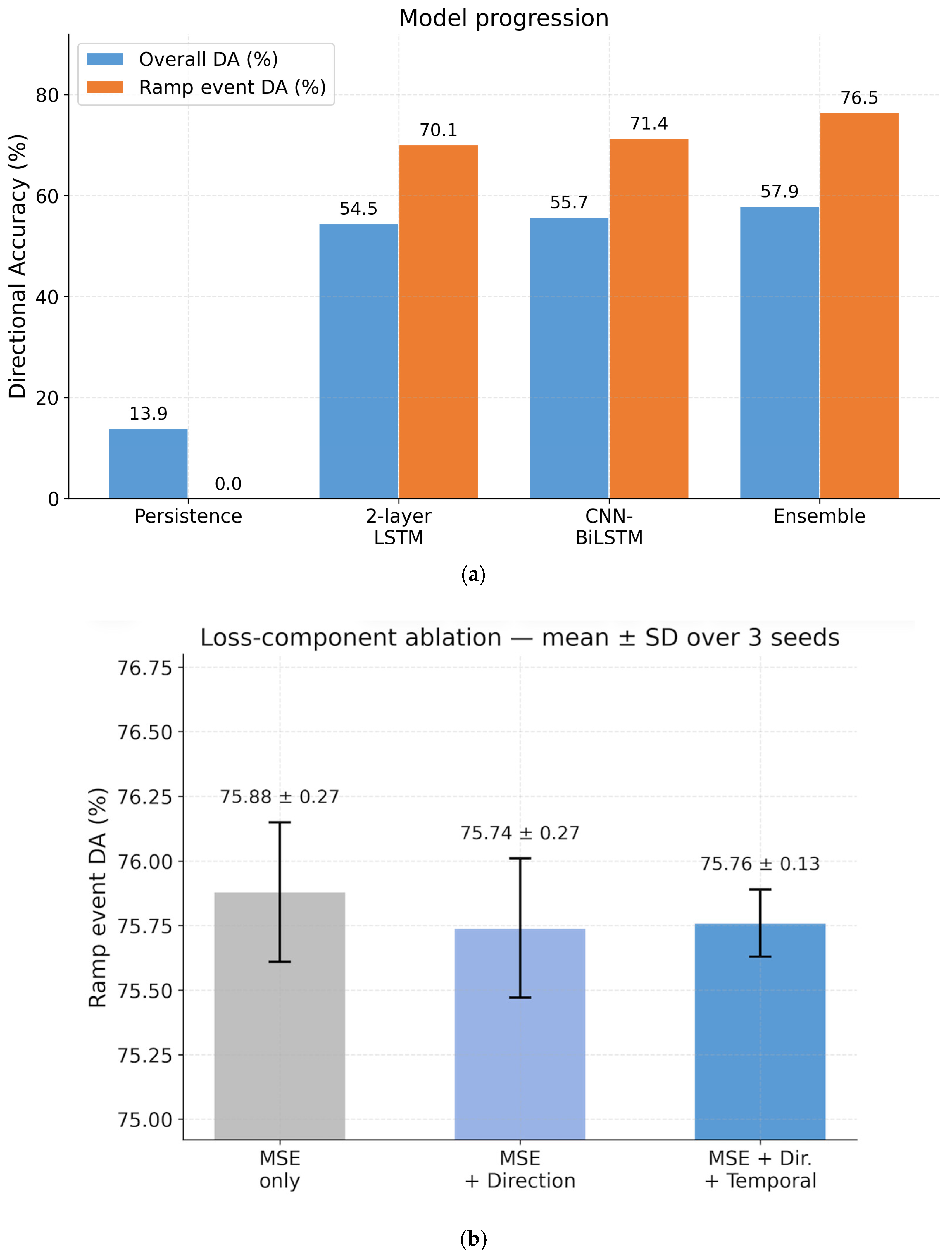
Figure 7a shows the model progression from persistence to ensemble in terms of both overall DA and ramp-DA. The ramp-DA progression (0.0% → 70.1% → 71.4% → 76.5%) demonstrates that each architectural advancement contributes to ramp event performance. The overall DA progression (13.9% → 54.5% → 55.7% → 57.9%) is much more modest, confirming that ramp-DA is the more informative metric for evaluating the contribution of each stage. Figure 7b presents the loss-component ablation, centred on ramp-DA and retrained across three random seeds (Table 5). Reported as mean ± standard deviation over seeds, ramp-DA is 75.9 ± 0.3% (MSE only), 75.7 ± 0.3% (+direction) and 75.8 ± 0.1% (+direction + temporal); stable-DA, WDA and overall DA are likewise flat to within their run-to-run standard deviation, and the best configuration differs from seed to seed. The one consistent effect is on point accuracy: the MSE-only configuration attains the lowest MAE in all three seeds (0.0908 ± 0.0009 versus 0.0930 ± 0.0016 and 0.0938 ± 0.0006). We therefore report the loss-component contribution as a candid null result at the ensemble scale and attribute the ensemble’s ramp-DA advantage to the regime-stratified specialist design and per-specialist weight tuning, rather than to any single auxiliary loss term; the direction-focused loss reshapes the per-specialist error profile during training, but does not, on its own, produce a statistically distinguishable ramp-DA gain once the specialists are combined.
Figure 7.
Model progression and loss-component ablation. (a) model progression showing overall DA (blue) and ramp event DA (orange) from persistence to ensemble. The ramp-DA progression (+76.5 pp from persistence) dwarfs the overall DA progression (+44.0 pp), confirming that aggregate metrics understate the ramp-focused contribution. (b) three-seed loss-component ablation (MSE only; +direction; +direction + temporal), with bars showing mean ramp-DA, and error bars showing the standard deviation over seeds 42, 123 and 2024. The three configurations are statistically indistinguishable on ramp-DA (differences below the run-to-run standard deviation); the MSE-only configuration attains the lowest MAE in every seed.
Domain-filtered niche evaluations were found to be sensitive to the choice of regime-defining thresholds and are therefore not reported as primary results. The specialist ramp-DA values in Table 2, computed on the common ramp definition (|ΔP| > 0.05 p.u.), provide a threshold-independent measure of the value of regime specialisation: the wide-context and multi-scale sub-models reach 67.2% and 76.1% ramp-DA respectively. The short-window sub-model scores below the 50% random-direction baseline on high-turbulence intervals, consistent with the fundamental stochasticity of turbulence at 10 min resolution (Section 7.2).
6.7. Prediction Interval (PI) Calibration
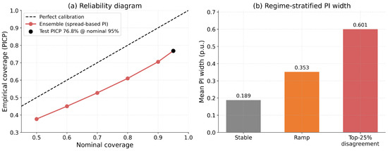
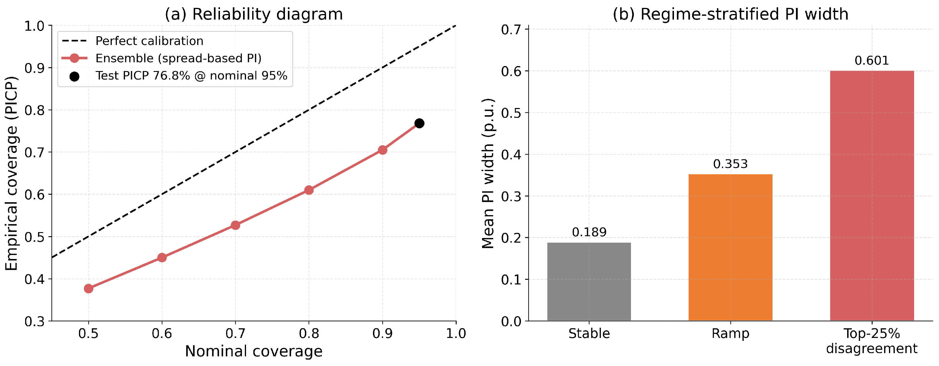
Figure 8 shows the prediction-interval reliability diagram and regime-stratified PI width. The ensemble intervals, constructed as the ensemble mean ±ζ·σ_ens(t) with ζ = 2.25 calibrated to 95% nominal coverage on the validation set, systematically under-cover on the test set (PICP = 76.8% at nominal 95%, falling to 37.7% at nominal 50%). This under-coverage of the spread-based intervals is expected and is addressed through conformal calibration as future work (Section 7.2). The PI width is, however, strongly regime-adaptive: mean width rises from 0.189 p.u. during stable periods to 0.353 p.u. during ramp events and 0.601 p.u. in the highest-uncertainty quartile (largest ensemble disagreement), so operators receive substantially wider intervals precisely when forecast uncertainty is greatest. We emphasise, moreover, that this regime adaptivity pertains to the comparative breadth of the intervals, rather than their absolute calibration: at the nominal 95% level, the spread-based intervals encompass merely 76.8% of test results. Consequently, they can be identified as informative, regime-sensitive uncertainty indicators, valuable for ranking intervals by relative risk.
Figure 8.
Prediction-interval calibration. (a) reliability diagram (empirical vs. nominal coverage) for the ensemble spread-based intervals, which systematically under-cover at every nominal level; intervals at non-95% nominal levels are obtained by Gaussian scaling of the validation-calibrated ζ. (b) mean PI width by regime, showing strong regime adaptation: narrowest during stable periods (0.189 p.u.), wider during ramps (0.353 p.u.), and widest in the highest ensemble disagreement quartile (0.601 p.u.).
6.8. One Farm Validation
To test cross-site generalisation without the small early-farm overlap present in the main split (Section 3.1), we retrained the five specialists (retaining their tuned hyperparameters) and the 2-layer LSTM baseline exclusively on Farms A and B, fitting the feature scaler on the A + B training portion alone, excluding lookback windows that cross the farm boundary, and evaluated on the entirety of Farm C (74,173 samples; 42.8% ramp prevalence). To keep the experiment tractable, the epoch budget was capped at 300 (versus up to 1000 in the main configuration), and pooled hyperparameters were reused.
In absolute terms, the transfer is strong because on the fully unseen farm the ensemble attains 77.4% ramp-DA and 64.4% overall DA, comparable to its within-region ramp-DA, and the five specialists converge to within one percentage point of one another (63.5–64.4% overall DA; 75.4–77.3% ramp-DA). However, the ensemble’s within-region advantage over the recurrent baseline does not transfer under this reduced-budget protocol: a paired bootstrap gives a small but significant overall DA deficit relative to the LSTM (−0.27 pp, 95% CI [−0.49, −0.05]) and a non-significant ramp-DA difference (+0.12 pp, 95% CI [−0.13, +0.37]). It shows that the framework generalises to an unseen site in absolute terms, while scoping the ensemble’s measured advantage over single-architecture baselines to the within-region setting.
7. Discussion
7.1. Operational Interpretation of the Ramp-DA Gain
The +6.4 pp ramp-DA improvement (70.1% → 76.5%) translates to approximately 985 fewer missed ramp event directions over the six-month test period per farm, derived as follows: 6.4% × 15,396 ramp event test samples = 985 fewer incorrect directions per six months, scaling to approximately 1970 per year. The operational value of this improvement is most appropriately expressed through the documented cost of wind imbalance energy, rather than a fixed per-event penalty. An empirical analysis of the Portuguese balancing market reports wind balancing costs of approximately 2 €/MWh of generated energy (an average of about 2.17 €/MWh over 2012–2016), derived from actual transmission system operator settlement data [25]; costs in other European markets may differ with grid strength and market design. Each correctly anticipated ramp direction reduces the imbalance energy that must be covered by reserves on the corresponding side of the ramp, so a sustained gain in ramp direction accuracy lowers the volume of wind generation settled at imbalance prices and the associated reserve deployment cost. The 19.1% MAE reduction compounds this benefit by tightening reserve margins on both sides of the ramp. The magnitude of the resulting saving scales with each farm’s annual energy throughput and its local imbalance price exposure, and a site-specific quantification is left to future work; the direction of the effect, however, is consistent with the established economic value of improved wind power forecasting demonstrated in production cost studies [26]. The modest overall directional accuracy improvement (+3.4 pp) is the expected consequence of a ramp-focused design, rather than a deficiency of it. Stable intervals, characterised by minimal step-to-step variation in power output, constitute the majority of the test set, yet carry comparatively low operational significance: a directional error during a near-constant interval does not precipitate the reserve deployment actions that a mistimed or misdirected ramp forecast does. Aggregate accuracy is therefore dominated by the regime in which forecast errors are least consequential, which is precisely why it understates the operational value of a model optimised for ramp events. A model that gains 6.4 pp ramp-DA while maintaining stable-period accuracy (stable-DA 42.0% vs. 41.3% for the LSTM) is making the right operational trade-off: the modest overall DA gain reflects the dominance of stable intervals in the test set, not a degradation of them.
We recommend that forthcoming publications focused on grid-integration applications present ramp-DA as a key metric, in conjunction with aggregate accuracy and the recognised event-based classification metrics (recall, precision, F1, Critical Success Index), and clearly specify whether the model is intended for stable-period accuracy, ramp accuracy, or both. Ramp-DA answers a question that classification metrics overlook: “given that a ramp occurs, is its direction predicted correctly?”.
7.2. Limitations
7.2.1. Geographical Generalizability and Climate Specificity
The empirical validation in this study relies on data from three onshore wind farms in the Eastern Mediterranean (Peloponnese, Greece). This region is characterised by a strongly diurnal wind resource driven by thermal and sea-breeze cycles, resulting in a test set with a 46.1% ramp event prevalence, which is high relative to the values commonly reported for Northern European continental or offshore datasets. We note that ramp prevalence is strongly dependent on the ramp definition and site climatology and is therefore not directly comparable across studies. Consequently, the performance of specific sub-models, particularly the diurnal-scale sub-model, is highly optimised for this distinct climatology. While the absolute performance metrics (such as the 76.5% ramp-DA) reflect this specific environment, the underlying methodological framework is domain-agnostic. Adapting this system to an offshore environment, such as the North Sea, would not require discarding the architecture; rather, it would entail recalibrating the specialist ensemble to reflect local meteorological drivers, for instance, allocating greater learning capacity to the wide-context sub-model (synoptic regimes) over the diurnal-scale one. Consequently, while the absolute performance metrics reflect the specific diurnal regime of our test sites, the core innovations, regime-stratified training and operational evaluation constitute a flexible methodology. Adapting it to other geographic or climatic profiles requires only redefining the specialist categories and retraining on local data, not altering the framework itself.
A second limitation concerns the meteorological inputs. The model relies solely on on-site SCADA measurements of wind speed and active power; it does not ingest any exogenous meteorological context such as numerical weather prediction (NWP) fields, reanalysis data, or upstream observations. This keeps the pipeline fully operational and causal, since every feature is computed from past on-site measurements available in real time, but it also means the model cannot anticipate ramps whose precursors are synoptic and not yet visible in the local wind signal (for example, an approaching front several hours ahead). Incorporating short-range NWP forecasts as an additional input is therefore expected to improve longer-horizon, frontal-passage ramp prediction, and we identify this as an important direction for future work (Section 8).
7.2.2. PI Calibration Gap
The PICP = 76.8% at nominal 95% reflects the limitations of the spread-based intervals used here, constructed as the ensemble mean ±ζ·σ_ens(t) with ζ calibrated to 95% nominal coverage on the validation set. Because this construction assumes the validation-period relationship between ensemble spread and error transfers unchanged to the test period, it under-covers under the seasonal and regime-dependent distribution shift between the validation and test periods. We emphasise that these intervals are not conformal and carry no coverage guarantee; the observed 18-point shortfall is consistent with this. Standard split-conformal prediction would guarantee marginal coverage only under exchangeability, an assumption that is violated for autocorrelated, non-stationary wind power series, so a naive conformal layer would not by itself resolve the gap. Closing it properly requires a time-series-valid procedure, such as adaptive conformal inference [27] or ensemble batch prediction intervals, that maintains coverage under distribution shift. We consequently disclose the calibration gap openly, instead of asserting valid coverage, and regard accurate time-series conformal calibration as prospective work (Section 8), rather than an established element of the current system. In the meantime, these spread-based intervals are expected to be perceived as informative, regime-sensitive indicators of uncertainty, rather than dependable confidence intervals for immediate dispatch decisions; their practical significance resides in signalling elevated uncertainty (relative width), not in assuring a specific coverage level (absolute calibration).
7.2.3. Turbulence Predictability Ceiling
The short-window sub-model’s niche DA on the 217 highest-turbulence test samples falls below the 50% random-direction baseline. This is physically expected under the Kolmogorov turbulence cascade [28], in which energy transfer to ever-smaller scales renders sub-grid turbulent fluctuations effectively stochastic at 10 min resolution, so any confident directional prediction during high-turbulence intervals is likely wrong. The short-window sub-model’s role within the ensemble is therefore prediction-interval inflation, and its disagreement with other specialists widens the ensemble PI during high-turbulence intervals, correctly signalling elevated uncertainty to grid operators. This niche DA is excluded from primary result tables.
7.2.4. Persistence TPA Artefact
Persistence achieves TPA = 99.2% because it always predicts no change, so any transition from stable to ramp counts as a correctly timed “turning point prediction” under the definition used. This artefact is why TPA alone is insufficient and must be reported alongside ramp-DA.
8. Future Work
Four high-priority directions will be pursued in future work: (i) Time-series-valid conformal post-processing (for example, adaptive conformal inference or ensemble batch prediction intervals) to close the PI calibration gap under distribution shift, since standard exchangeability-based conformal prediction is not directly valid for these non-stationary, autocorrelated series. (ii) Integration of transformer architectures (e.g., PatchTST, iTransformer) as additional specialists within the ensemble. (iii) Transfer learning experiments on Northern European offshore sites to characterise generalisation requirements. (iv) Integration of short-range NWP output as an additional input to the wide-context sub-model, expected to improve frontal-passage ramp prediction at horizons beyond 60 min. Reanalysis products such as ERA5 [29], together with operational short-range NWP, are the natural candidate sources of this exogenous meteorological context, which the present on-site-only model deliberately does not use.
9. Conclusions
We have presented a ramp event-focused wind power forecasting framework with two core contributions: a regime-stratified evaluation methodology that reveals model behaviour obscured by aggregate metrics, and a specialist ensemble whose regime-stratified design concentrates modelling capacity on operationally critical ramp event intervals, trained with a direction-focused loss that makes directional error explicit during optimisation. As wind penetration rises and system inertia falls, the cost of a missed ramp direction grows more sharply than the cost of average forecast error, making the metric reframing proposed here increasingly consequential for grid security, not merely a methodological preference.
On 33,411 held-out samples from three Greek wind farms, the ensemble achieves 76.5% ramp event DA, a statistically confirmed +6.4 pp over the LSTM baseline (DM p < 0.001; ensemble ramp-DA 95% CI [75.8, 77.1]%, seeded percentile bootstrap), a margin that also holds against the PatchTST and iTransformer baselines (paired bootstrap +2.2 and +2.4 pp, both significant). The overall DA of 57.9% (+3.4 pp vs. LSTM) is modest by design: the regime-stratified specialist ensemble concentrates modelling capacity on ramp intervals, rather than on aggregate accuracy, and the weighted DA (82.2%) confirms the gains are concentrated where they matter. As the loss-component ablation shows (Section 6.6), the direction-focused loss reshapes each specialist’s training but is not, on its own, the source of the ensemble’s ramp-DA advantage. The specialist design is supported by the threshold-independent specialist ramp-DA values (Table 2), with the wide-context and multi-scale sub-models reaching 67.2% and 76.1% respectively, while the short-window sub-model’s niche DA falls below the 50% random-direction baseline, correctly reflecting an irreducible physical predictability limit at 10 min resolution. Empirical evidence confirms the central methodological claim that ramp event DA should be used as a primary metric for grid-integration-focused forecasting papers, along with aggregate accuracy and event-detection metrics. The +6.4 pp ramp-DA improvement is nearly twice the +3.4 pp overall DA improvement, indicating that aggregate metrics understate the operational value of this architecture.
We invite the community to adopt regime-stratified evaluation as standard practice for grid-integration forecasting, and offer the results reported here (and the openly released implementation) as a reproducible baseline for Eastern Mediterranean onshore wind. Finally, the regime-stratified evaluation principle is not specific to wind: any forecasting problem in which rare, high-consequence transitions are diluted by an easy-to-predict majority (load spikes, price jumps, demand ramps) is susceptible to the same aggregate-metric blind spot this work exposes and stands to benefit from the same regime-stratified treatment.
Author Contributions
Conceptualization, K.S. and T.E.K.; Methodology, K.S. and T.E.K.; Software, K.S.; Investigation, K.S.; Data curation, K.S.; Writing—original draft, K.S.; Writing—review & editing, T.E.K.; Visualization, K.S.; Supervision, T.E.K. All authors have read and agreed to the published version of the manuscript.
Funding
The research is conducted in the operating framework of the University of Thessaly Innovation, Technology Transfer Unit and Entrepreneurship Center “One Planet Thessaly”, under the “University of Thessaly Grants for Scientific Publication Support” action and is funded by the Special Account of Research Grants of the University of Thessaly.
Data Availability Statement
The SCADA operational data (wind speed and active power) that support the findings of this study were provided by TERNA Energy S.A. under a research data use agreement and are subject to commercial confidentiality; they are therefore not publicly available, but may be obtained from the authors with the permission of TERNA Energy S.A. on reasonable request. The model implementation, training configurations, quality-control pipeline, and feature-engineering and evaluation scripts are openly available at https://github.com/Scientifico32/Ramp-Event-Forecasting (accessed on 2 June 2026), supporting reproducibility will be made available in a public repository upon publication to support reproducibility of all components that do not depend on the proprietary SCADA records.
Acknowledgments
SCADA data were provided by TERNA Energy S.A. under a research data use agreement. The authors thank TERNA Energy for granting access to the wind farm operational records used in this study.
Conflicts of Interest
The funders had no role in the design of the study; in the collection, analyses, or interpretation of data; in the writing of the manuscript; or in the decision to publish the results.
Abbreviations
The following abbreviations are used in this manuscript:
| CI | Confidence Interval |
| CNN | Convolutional Neural Network |
| CNN-BiLSTM | Convolutional Neural Network–Bidirectional Long Short-Term Memory |
| CSI | Critical Success Index |
| DA | Directional Accuracy |
| DM | Diebold–Mariano (test) |
| GPU | Graphics Processing Unit |
| GRU | Gated Recurrent Unit |
| LSTM | Long Short-Term Memory |
| MAE | Mean Absolute Error |
| MSE | Mean Squared Error |
| NWP | Numerical Weather Prediction |
| PI | Prediction Interval |
| PICP | Prediction Interval Coverage Probability |
| PINN | Physics-Informed Neural Network |
| Ramp-DA | Ramp event Directional Accuracy |
| RMSE | Root Mean Squared Error |
| SCADA | Supervisory Control and Data Acquisition |
| Stable-DA | Stable-period Directional Accuracy |
| TPA | Turning Point Accuracy |
| WDA | Weighted Directional Accuracy |
References
- Makarov, Y.V.; Etingov, P.; Ma, J.; Huang, Z.; Subbarao, K. Incorporating uncertainty of wind power generation forecast into power system operation, dispatch, and unit commitment procedures. IEEE Trans. Sustain. Energy 2011, 2, 433–442. [Google Scholar] [CrossRef] [Scilit]
- Banakar, H.; Luo, C.; Ooi, B.-T. Impacts of wind power minute-to-minute variations on power system operation. IEEE Trans. Power Syst. 2008, 23, 150–160. [Google Scholar] [CrossRef] [Scilit]
- Cui, Y.; Chen, Z.; He, Y.; Xiong, X.; Li, F. An algorithm for forecasting day-ahead wind power via novel long short-term memory and wind power ramp events. Energy 2023, 263, 125888. [Google Scholar] [CrossRef] [Scilit]
- Ahn, E.J.; Hur, J. A practical metric to evaluate the ramp events of wind generating resources to enhance the security of smart energy systems. Energies 2022, 15, 2676. [Google Scholar] [CrossRef] [Scilit]
- Pichault, M.; Vincent, C.L.; Skidmore, G.; Monty, J. Characterisation of intra-hourly wind power ramps at the wind farm scale and associated processes. Wind Energy Sci. 2021, 6, 131–147. [Google Scholar] [CrossRef] [Scilit]
- Bossavy, A.; Girard, R.; Kariniotakis, G. Forecasting ramps of wind power production with numerical weather prediction ensembles. Wind Energy 2013, 16, 51–63. [Google Scholar] [CrossRef] [Scilit]
- Bianco, L.; Djalalova, I.V.; Wilczak, J.M.; Cline, J.; Calvert, S.; Konopleva-Akish, E.; Finley, C.; Freedman, J. A wind energy ramp tool and metric for measuring the skill of numerical weather prediction models. Weather Forecast. 2016, 31, 1137–1156. [Google Scholar] [CrossRef] [Scilit]
- Ferreira, C.; Gama, J.; Matias, L.; Botterud, A.; Wang, J. A Survey on Wind Power Ramp Forecasting (Report ANL/DIS-10-13); Argonne National Laboratory: Argonne, IL, USA, 2011. [CrossRef] [Scilit]
- Madsen, H.; Pinson, P.; Kariniotakis, G.; Nielsen, H.A.; Nielsen, T.S. Standardizing the performance evaluation of short-term wind power prediction models. Wind Eng. 2005, 29, 475–489. [Google Scholar] [CrossRef] [Scilit]
- Zhang, J.; Zhu, X.; Xie, Y.; Chen, G.; Liu, S. Detection and prediction of wind and solar photovoltaic power ramp events based on data-driven methods: A critical review. Energies 2025, 18, 3290. [Google Scholar] [CrossRef] [Scilit]
- Gallego-Castillo, C.; Cuerva-Tejero, A.; Lopez-Garcia, O. A review on the recent history of wind power ramp forecasting. Renew. Sustain. Energy Rev. 2015, 52, 1148–1157. [Google Scholar] [CrossRef] [Scilit]
- Pinson, P.; Madsen, H. Adaptive modelling and forecasting of offshore wind power fluctuations with Markov-switching autoregressive models. J. Forecast. 2010, 31, 281–313. [Google Scholar] [CrossRef] [Scilit]
- Peng, X.; Li, Y.; Tsung, F. A graph attention network with spatio-temporal wind propagation graph for wind power ramp events prediction. Renew. Energy 2024, 236, 121280. [Google Scholar] [CrossRef] [Scilit]
- Gallego, C.; Costa, A.; Cuerva, A. Improving short-term forecasting during ramp events by means of Regime-Switching Artificial Neural Networks. Adv. Sci. Res. 2011, 6, 55–58. [Google Scholar] [CrossRef] [Scilit]
- Han, L.; Qiao, Y.; Li, M.; Shi, L. Wind power ramp event forecasting based on feature extraction and deep learning. Energies 2020, 13, 6449. [Google Scholar] [CrossRef] [Scilit]
- Ren, G.; Wan, J.; Wang, Y.; Yao, K.; Fu, J.; Yu, J. A direct prediction method for wind power ramp events considering the class imbalanced problem. Energy Sci. Eng. 2023, 11, 1705–1715. [Google Scholar] [CrossRef] [Scilit]
- Cui, M.; Ke, D.; Sun, Y.; Gan, D.; Zhang, J.; Hodge, B.-M. Wind power ramp event forecasting using a stochastic scenario generation method. IEEE Trans. Sustain. Energy 2015, 6, 422–433. [Google Scholar] [CrossRef] [Scilit]
- Trombe, P.-J.; Pinson, P.; Madsen, H. A general probabilistic forecasting framework for offshore wind power fluctuations. Energies 2012, 5, 621–657. [Google Scholar] [CrossRef] [Scilit]
- Valldecabres, L.; von Bremen, L.; Kühn, M. Minute-scale detection and probabilistic prediction of offshore wind turbine power ramps using dual-Doppler radar. Wind Energy 2020, 23, 2202–2224. [Google Scholar] [CrossRef] [Scilit]
- Zhang, X.; Li, T.; Yang, Q.; Zhou, X.; Benini, E. A novel non-dimensional multiple operating conditions physics-informed neural networks for wind turbine wake and power prediction in complex terrains. Energy 2026, 358, 141301. [Google Scholar] [CrossRef] [Scilit]
- Hu, J.; Zhang, L.; Tang, J.; Liu, Z. A novel transformer ordinal regression network with label diversity for wind power ramp events forecasting. Energy 2023, 280, 128075. [Google Scholar] [CrossRef] [Scilit]
- Nie, Y.; Nguyen, N.H.; Sinthong, P.; Kalagnanam, J. A time series is worth 64 words: Long-term forecasting with transformers. In Proceedings of the International Conference on Learning Representations (ICLR 2023), Kigali, Rwanda, 1–5 May 2023. [Google Scholar] [CrossRef] [Scilit]
- Liu, Y.; Hu, T.; Zhang, H.; Wu, H.; Wang, S.; Ma, L.; Long, M. ITransformer: Inverted transformers are effective for time series forecasting. In Proceedings of the International Conference on Learning Representations (ICLR 2024), Vienna, Austria, 7–11 May 2024. [Google Scholar] [CrossRef] [Scilit]
- Angelopoulos, A.N.; Bates, S. Conformal prediction: A gentle introduction. Found. Trends Mach. Learn. 2023, 16, 494–591. [Google Scholar] [CrossRef] [Scilit]
- Frade, P.M.S.; Pereira, J.P.; Santana, J.J.E.; Catalão, J.P.S. Wind balancing costs in a power system with high wind penetration—Evidence from Portugal. Energy Policy 2019, 132, 702–713. [Google Scholar] [CrossRef] [Scilit]
- Wang, Q.; Martinez-Anido, C.B.; Wu, H.; Florita, A.R.; Hodge, B.-M. Quantifying the economic and grid reliability impacts of improved wind power forecasting. IEEE Trans. Sustain. Energy 2016, 7, 1525–1537. [Google Scholar] [CrossRef] [Scilit]
- Gibbs, I.; Candès, E. Adaptive conformal inference under distribution shift. Adv. Neural Inf. Process. Syst. 2021, 34, 1660–1672. [Google Scholar] [CrossRef] [Scilit]
- Monin, A.S.; Yaglom, A.M. Statistical Fluid Mechanics: Mechanics of Turbulence; MIT Press: Cambridge, MA, USA, 1975; Volume 2. [Google Scholar]
- Hersbach, H.; Bell, B.; Berrisford, P.; Hirahara, S.; Horányi, A.; Muñoz-Sabater, J.; Nicolas, J.; Peubey, C.; Radu, R.; Schepers, D.; et al. The ERA5 global reanalysis. Q. J. R. Meteorol. Soc. 2020, 146, 1999–2049. [Google Scholar] [CrossRef] [Scilit]

Disclaimer/Publisher’s Note: The statements, opinions and data contained in all publications are solely those of the individual author(s) and contributor(s) and not of MDPI and/or the editor(s). MDPI and/or the editor(s) disclaim responsibility for any injury to people or property resulting from any ideas, methods, instructions or products referred to in the content. |
© 2026 by the authors. Licensee MDPI, Basel, Switzerland. This article is an open access article distributed under the terms and conditions of the Creative Commons Attribution (CC BY) license.