Author Contributions
Conceptualization, K.S. and T.E.K.; Methodology, K.S. and T.E.K.; Software, K.S.; Investigation, K.S.; Data curation, K.S.; Writing—original draft, K.S.; Writing—review & editing, T.E.K.; Visualization, K.S.; Supervision, T.E.K. All authors have read and agreed to the published version of the manuscript.
Figure 1.
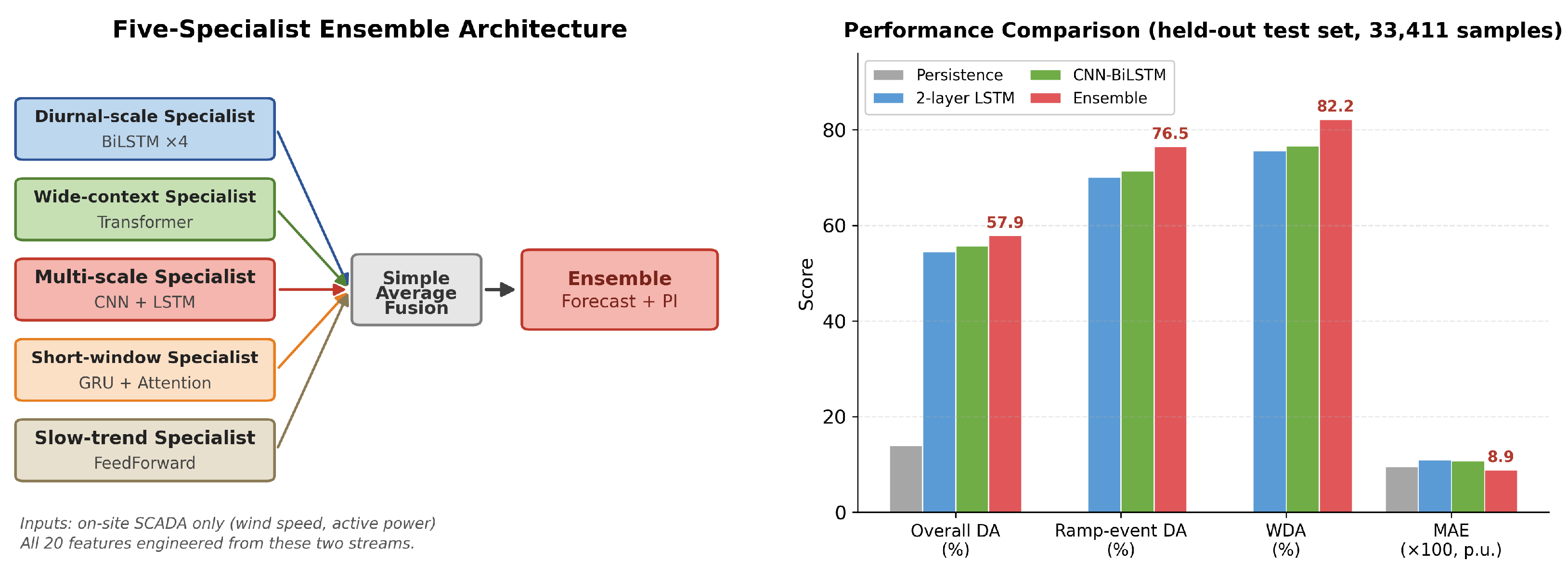
Ensemble architecture and performance summary. (Left) five-specialist mixture-of-experts design with simple average fusion. (Right) performance comparison across all models on the held-out test set (33,411 samples). The ramp event DA column (second from left) shows the primary contribution: a +6.4 pp ramp-DA improvement over the LSTM baseline. The ensemble’s forecast error advantage over the LSTM is statistically significant by a Diebold–Mariano test on the absolute-error differential of the 10 min series.
Figure 1.
Ensemble architecture and performance summary. (Left) five-specialist mixture-of-experts design with simple average fusion. (Right) performance comparison across all models on the held-out test set (33,411 samples). The ramp event DA column (second from left) shows the primary contribution: a +6.4 pp ramp-DA improvement over the LSTM baseline. The ensemble’s forecast error advantage over the LSTM is statistically significant by a Diebold–Mariano test on the absolute-error differential of the 10 min series.
Figure 2.
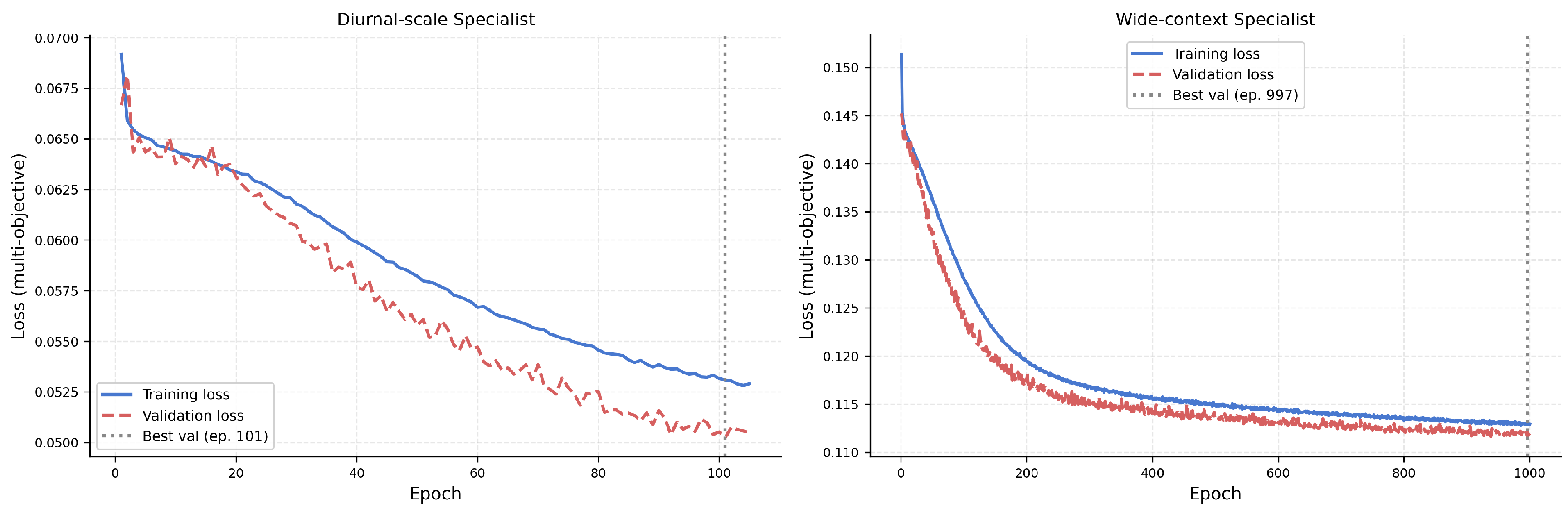
Training and validation loss curves for the diurnal-scale (left) and wide-context (right) sub-models.
Figure 2.
Training and validation loss curves for the diurnal-scale (left) and wide-context (right) sub-models.
Figure 3.
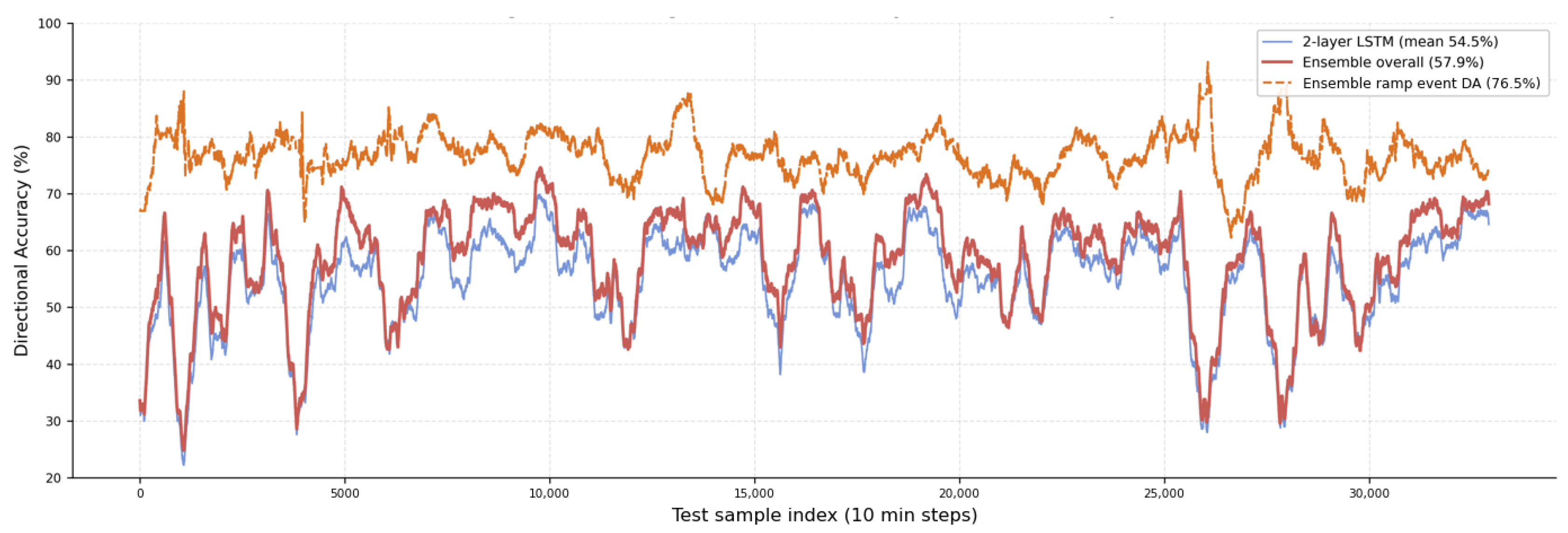
Rolling directional accuracy over the test set (window = 500 steps ≈ 3.5 days). The ensemble ramp event DA (orange dashed, mean 76.5%) is consistently and substantially elevated above the overall ensemble DA (red solid, mean 57.9%) and the LSTM (blue, mean 54.5%), confirming that the regime-stratified advantage is stable across all seasons and weather patterns in the test period.
Figure 3.
Rolling directional accuracy over the test set (window = 500 steps ≈ 3.5 days). The ensemble ramp event DA (orange dashed, mean 76.5%) is consistently and substantially elevated above the overall ensemble DA (red solid, mean 57.9%) and the LSTM (blue, mean 54.5%), confirming that the regime-stratified advantage is stable across all seasons and weather patterns in the test period.
Figure 4.
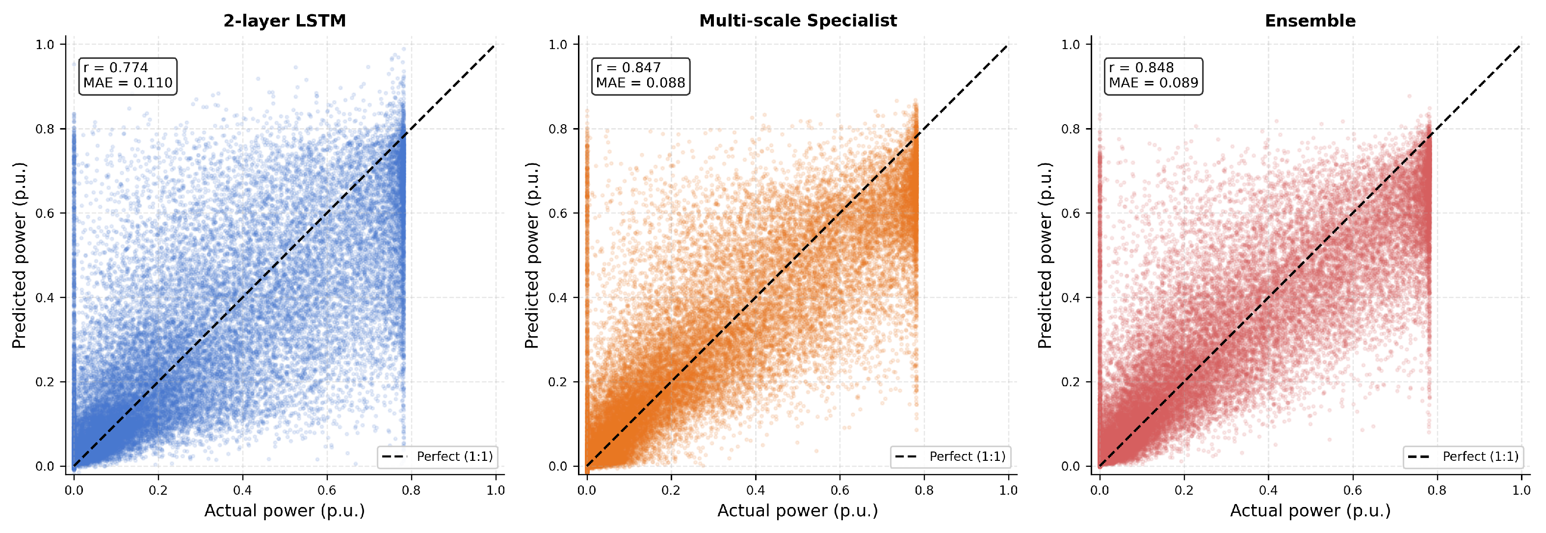
Predicted vs. actual wind power scatter plots (normalised, p.u.) for the 2-layer LSTM baseline (left, r = 0.774, MAE = 0.110), the multi-scale sub-model (centre, r = 0.847, MAE = 0.088), and the ensemble (right, r = 0.848, MAE = 0.089). Dispersion decreases systematically from LSTM to ensemble, particularly at intermediate power levels (0.2–0.6 p.u.) corresponding to ramp event transitions.
Figure 4.
Predicted vs. actual wind power scatter plots (normalised, p.u.) for the 2-layer LSTM baseline (left, r = 0.774, MAE = 0.110), the multi-scale sub-model (centre, r = 0.847, MAE = 0.088), and the ensemble (right, r = 0.848, MAE = 0.089). Dispersion decreases systematically from LSTM to ensemble, particularly at intermediate power levels (0.2–0.6 p.u.) corresponding to ramp event transitions.
Figure 5.
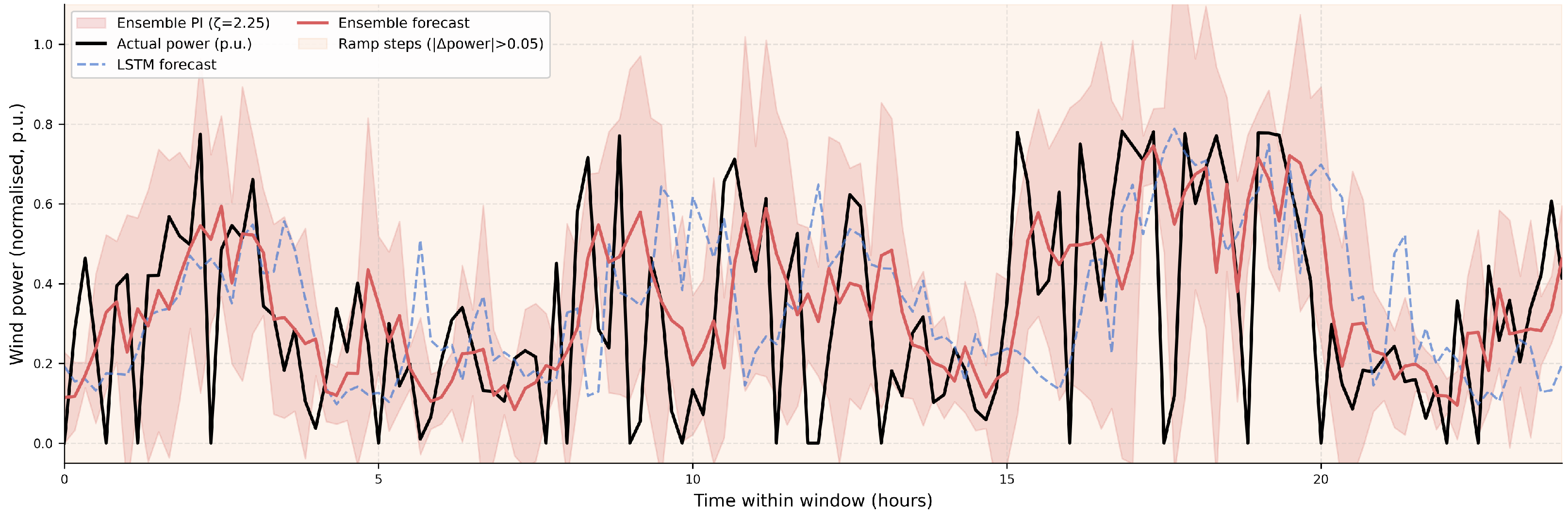
Forecast example over a ramp-dense window from the held-out test set. Black: actual power; red: ensemble forecast; blue dashed: LSTM; pink band: ensemble prediction interval (ζ = 2.25). The interval widens during high-disagreement periods.
Figure 5.
Forecast example over a ramp-dense window from the held-out test set. Black: actual power; red: ensemble forecast; blue dashed: LSTM; pink band: ensemble prediction interval (ζ = 2.25). The interval widens during high-disagreement periods.
Figure 6.
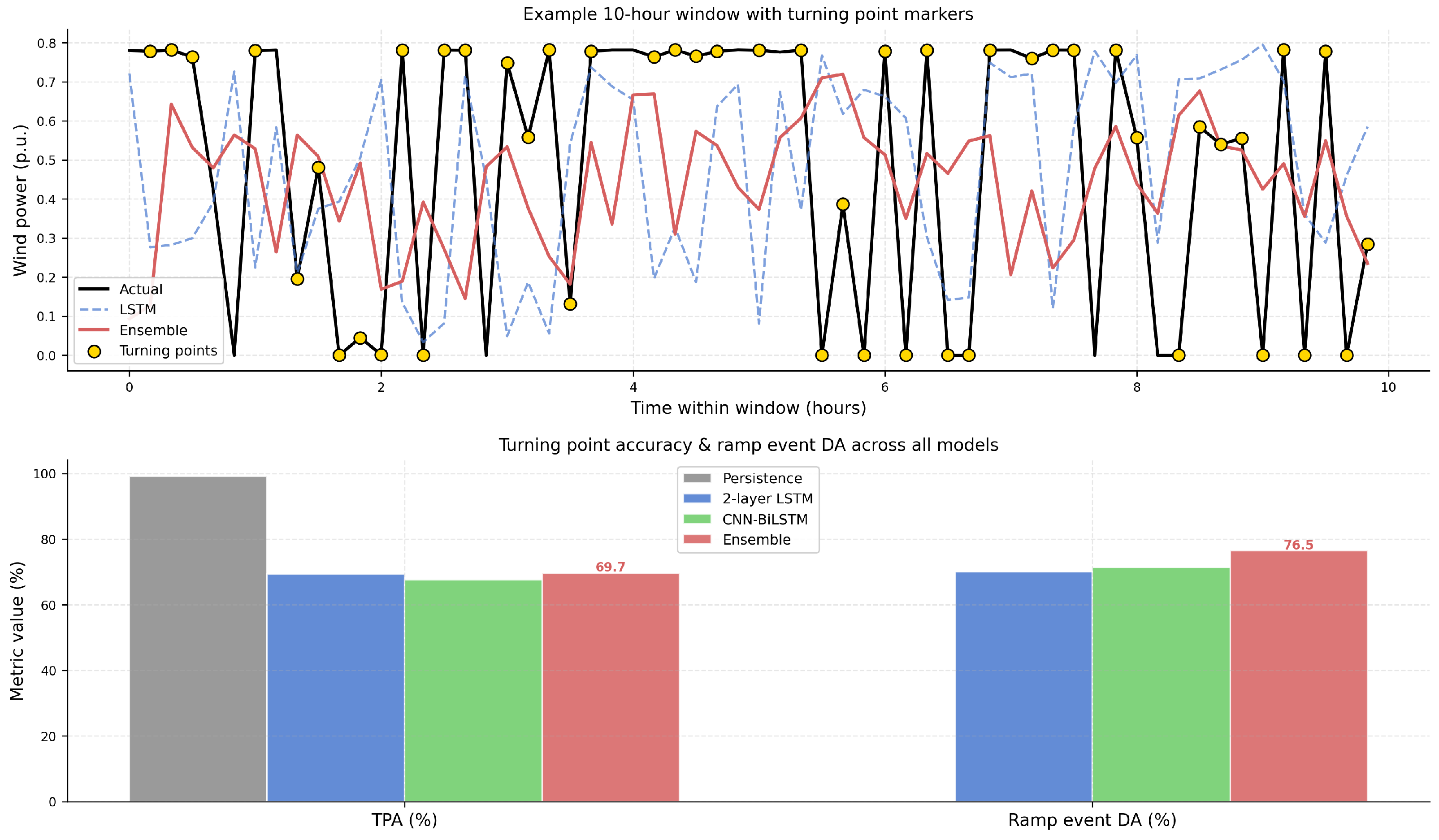
Turning point detection performance. Upper: example 10 h test window with actual turning point markers (gold), ensemble forecast (red), and LSTM forecast (blue dashed). Lower: TPA and ramp event DA across all models. Persistence TPA = 99.2% is a definitional artefact (see
Section 7.2); its ramp-DA = 0.0% confirms operational worthlessness during ramp events.
Figure 6.
Turning point detection performance. Upper: example 10 h test window with actual turning point markers (gold), ensemble forecast (red), and LSTM forecast (blue dashed). Lower: TPA and ramp event DA across all models. Persistence TPA = 99.2% is a definitional artefact (see
Section 7.2); its ramp-DA = 0.0% confirms operational worthlessness during ramp events.
Figure 7.
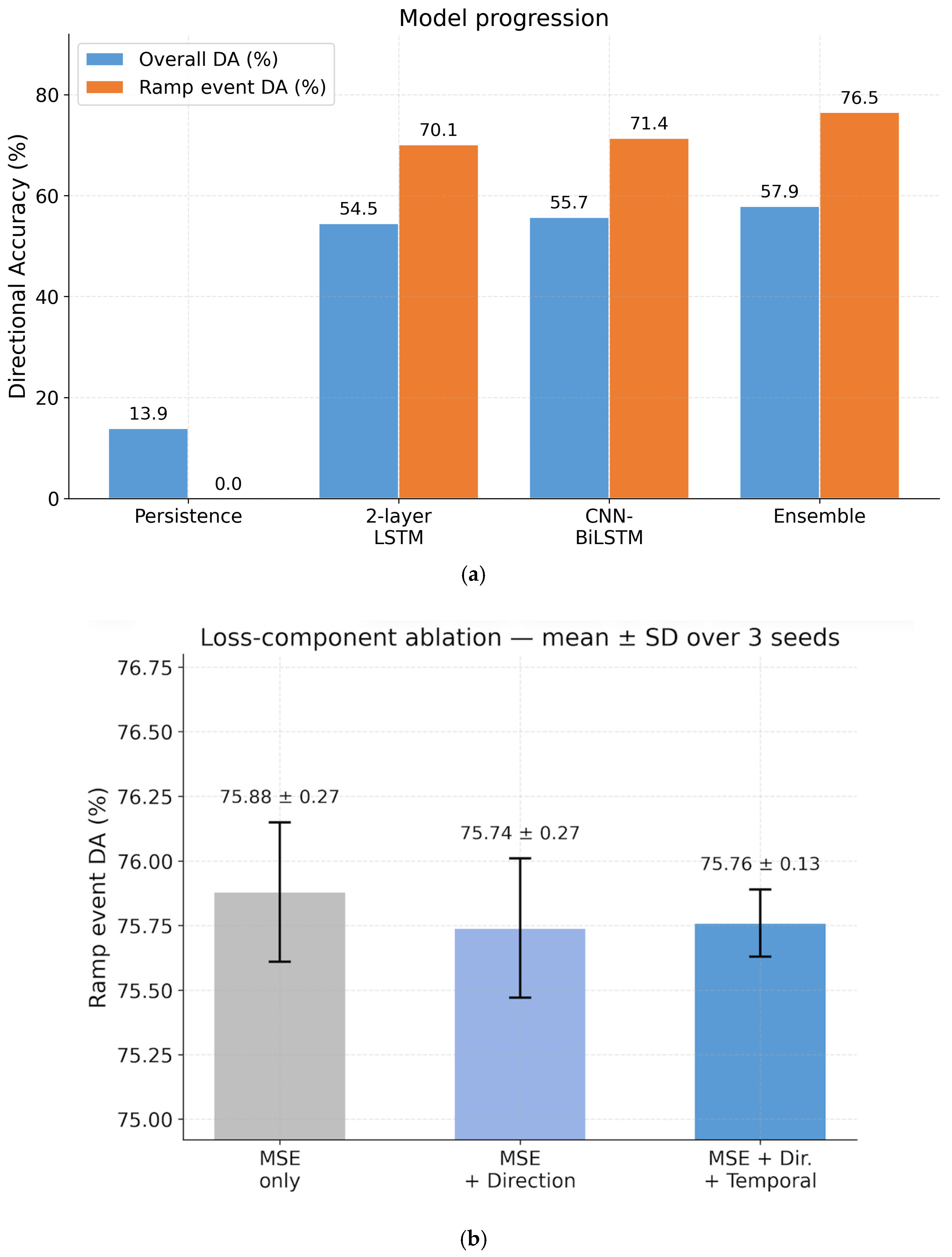
Model progression and loss-component ablation. (a) model progression showing overall DA (blue) and ramp event DA (orange) from persistence to ensemble. The ramp-DA progression (+76.5 pp from persistence) dwarfs the overall DA progression (+44.0 pp), confirming that aggregate metrics understate the ramp-focused contribution. (b) three-seed loss-component ablation (MSE only; +direction; +direction + temporal), with bars showing mean ramp-DA, and error bars showing the standard deviation over seeds 42, 123 and 2024. The three configurations are statistically indistinguishable on ramp-DA (differences below the run-to-run standard deviation); the MSE-only configuration attains the lowest MAE in every seed.
Figure 7.
Model progression and loss-component ablation. (a) model progression showing overall DA (blue) and ramp event DA (orange) from persistence to ensemble. The ramp-DA progression (+76.5 pp from persistence) dwarfs the overall DA progression (+44.0 pp), confirming that aggregate metrics understate the ramp-focused contribution. (b) three-seed loss-component ablation (MSE only; +direction; +direction + temporal), with bars showing mean ramp-DA, and error bars showing the standard deviation over seeds 42, 123 and 2024. The three configurations are statistically indistinguishable on ramp-DA (differences below the run-to-run standard deviation); the MSE-only configuration attains the lowest MAE in every seed.
Figure 8.
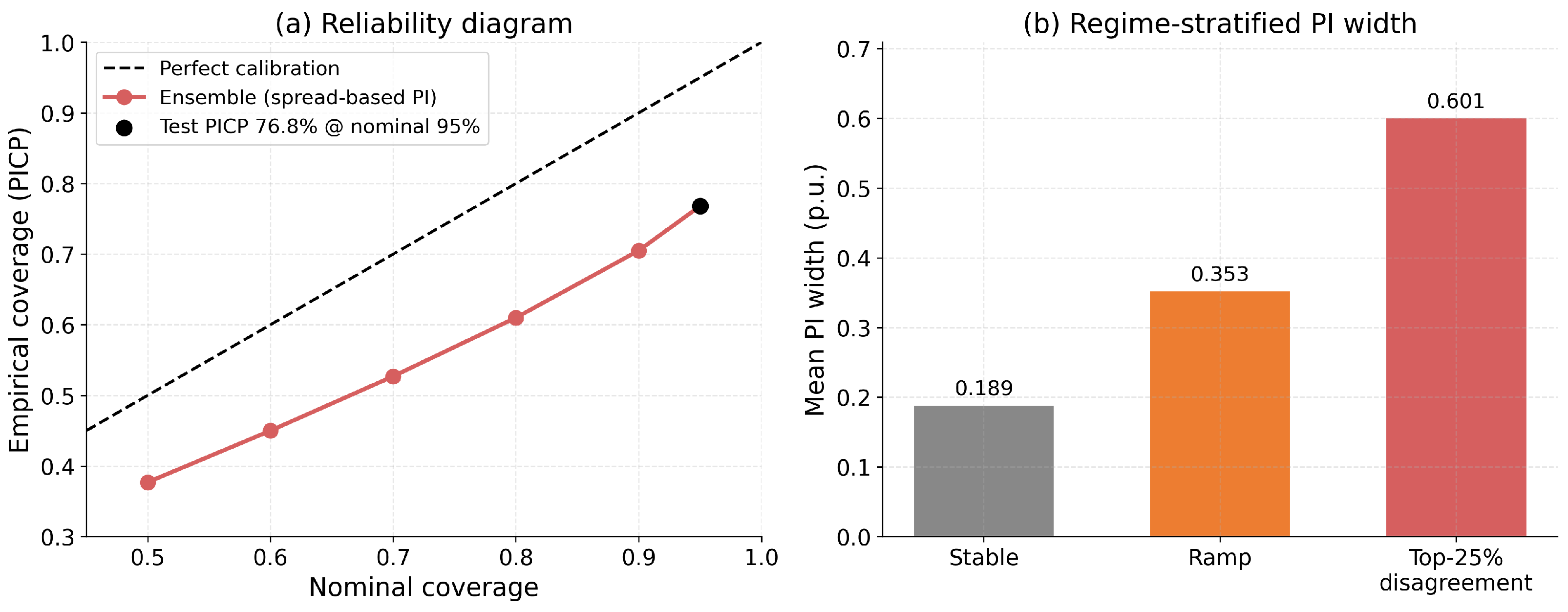
Prediction-interval calibration. (a) reliability diagram (empirical vs. nominal coverage) for the ensemble spread-based intervals, which systematically under-cover at every nominal level; intervals at non-95% nominal levels are obtained by Gaussian scaling of the validation-calibrated ζ. (b) mean PI width by regime, showing strong regime adaptation: narrowest during stable periods (0.189 p.u.), wider during ramps (0.353 p.u.), and widest in the highest ensemble disagreement quartile (0.601 p.u.).
Figure 8.
Prediction-interval calibration. (a) reliability diagram (empirical vs. nominal coverage) for the ensemble spread-based intervals, which systematically under-cover at every nominal level; intervals at non-95% nominal levels are obtained by Gaussian scaling of the validation-calibrated ζ. (b) mean PI width by regime, showing strong regime adaptation: narrowest during stable periods (0.189 p.u.), wider during ramps (0.353 p.u.), and widest in the highest ensemble disagreement quartile (0.601 p.u.).
Table 1.
Ramp threshold sensitivity (held-out test set, n = 33,411). As the |Δpower| threshold is tightened, prevalence falls and directional accuracy rises for both models.
Table 1.
Ramp threshold sensitivity (held-out test set, n = 33,411). As the |Δpower| threshold is tightened, prevalence falls and directional accuracy rises for both models.
| Threshold (p.u.) | Prevalence | n (Ramp) | Ensemble Ramp-DA | LSTM Ramp-DA | Margin |
|---|
| 0.05 | 46.1% | 15,396 | 76.5% | 70.1% | +6.4 pp |
| 0.10 | 29.7% | 9925 | 81.8% | 73.9% | +7.9 pp |
| 0.15 | 20.6% | 6880 | 85.8% | 77.9% | +7.9 pp |
| 0.20 | 14.7% | 4902 | 89.3% | 80.8% | +8.5 pp |
| 0.25 | 10.7% | 3576 | 91.3% | 83.3% | +8.0 pp |
Table 2.
Specialist sub-model architectures and ramp event directional accuracy on the held-out test set. Ensemble outperforms all individual specialists on ramp-DA (76.5%) while achieving the second-lowest MAE (0.089).
Table 2.
Specialist sub-model architectures and ramp event directional accuracy on the held-out test set. Ensemble outperforms all individual specialists on ramp-DA (76.5%) while achieving the second-lowest MAE (0.089).
| Specialist | Architecture | Target Regime | Ramp-DA (%) | MAE (p.u.) |
|---|
| Diurnal-scale | BiLSTM ×4 | Sea-breeze/diurnal | 73.8 | 0.095 |
| Wide-context | Transformer ×6 | Synoptic fronts | 67.2 | 0.123 |
| Multi-scale | CNN + LSTM | Orographic channelling | 76.1 | 0.088 |
| Short-window | GRU + Attention | Sub-hourly gusts | 73.8 | 0.094 |
| Slow-trend | FeedForward ×4 | Slow multi-hour ramps | 74.3 | 0.099 |
| Ensemble | Simple average | All regimes | 76.5 | 0.089 |
Table 3.
Full performance metrics for the test set (33,411 samples). Bold indicates the proposed ensemble.
Table 3.
Full performance metrics for the test set (33,411 samples). Bold indicates the proposed ensemble.
| Model | Overall DA (%) | Ramp-DA (%) | Stable-DA (%) | WDA (%) | MAE (p.u.) | r |
|---|
| Persistence | 13.9 | 0.0 | 25.7 | 0.0 | 0.096 | 0.792 |
| 2-layer LSTM | 54.5 | 70.1 | 41.3 | 75.6 | 0.110 | 0.774 |
| CNN-BiLSTM | 55.7 | 71.4 | 42.3 | 76.6 | 0.108 | 0.769 |
| PatchTST | 56.3 | 74.3 | 40.9 | 80.8 | 0.090 | 0.849 |
| iTransformer | 56.4 | 74.1 | 41.3 | 79.8 | 0.089 | 0.846 |
| Ensemble | 57.9 | 76.5 | 42.0 | 82.2 | 0.089 | 0.848 |
Table 4.
Paired percentile bootstrap differences.
Table 4.
Paired percentile bootstrap differences.
| Comparison | Δ Overall DA (pp, 95 CI) | Δ Ramp-DA (pp, 95% CI) |
|---|
| Ensemble—PatchTST | +1.61 [+1.17, +2.04] | +2.18 [+1.54, +2.78] |
| Ensemble—iTransformer | +1.50 [+1.10, +1.87] | +2.38 [+1.79, +2.96] |
| Ensemble—CNN-BiLSTM | +2.20 [+1.76, +2.63] | +5.12 [+4.44, +5.84] |
| Ensemble—LSTM | +3.35 [+2.90, +3.77] | +6.44 [+5.75, +7.12] |
Table 5.
Loss-component ablation centred on ramp-DA, mean ± standard deviation over three seeds (held-out test set; 15,396 ramp events). Directional metrics are flat to within the standard deviation; only MAE moves systematically, being lowest under MSE only.
Table 5.
Loss-component ablation centred on ramp-DA, mean ± standard deviation over three seeds (held-out test set; 15,396 ramp events). Directional metrics are flat to within the standard deviation; only MAE moves systematically, being lowest under MSE only.
| Configuration | Ramp-DA (%) | Stable-DA(%) | WDA (%) | Overall DA (%) | MAE (p.u) |
|---|
| MSE only | 75.88 ± 0.27 | 42.30 ± 0.12 | 80.98 ± 0.27 | 57.77 ± 0.15 | 0.0908 ± 0.0009 |
| +Direction | 75.74 ± 0.27 | 42.51 ± 0.08 | 81.13 ± 0.23 | 57.82 ± 0.11 | 0.0930 ± 0.0016 |
| +Direction +Temporal | 75.76 ± 0.13 | 42.27 ± 0.07 | 81.11 ± 0.25 | 57.70 ± 0.09 | 0.0938 ± 0.0006 |
Table 6.
Models trained on Farms A and B and evaluated on the entirety of the unseen Farm C.
Table 6.
Models trained on Farms A and B and evaluated on the entirety of the unseen Farm C.
| Model | Overall DA (%) | Ramp-DA (%) | Stable-DA (%) | MAE (p.u.) | r |
|---|
| Persistence | 1.0 | 0.0 | 1.8 | 0.088 | 0.801 |
| 2-layer LSTM | 64.67 | 77.25 | 55.27 | 0.079 | 0.866 |
| Ensemble | 64.42 | 77.37 | 54.73 | 0.081 | 0.867 |