


Abstract
Ensuring the safety and reliability of photovoltaic (PV) installations requires accurate electrical arc fault detection. This work presents a computational arc fault detection framework that combines fixed-length windowing, Fast Fourier Transform (FFT)-based features, and supervised machine learning classifiers. Data were acquired using an Arc Fault Circuit Interrupter (AFCI) test bench developed based on IEC 63027. Current and voltage signals were partitioned into 200-sample windows, DC-offset corrected, and Hann-windowed signals. Each window generated 204 statistical and spectral attributes used to train and evaluate Random Forest (RF), K-Nearest Neighbors (KNN), Multilayer Perceptron (MLP), and Convolutional Neural Network (CNN) models. Hyperparameters were tuned by grid search with TimeSeriesSplit cross-validation, comparing min–max normalization and Z–Score standardization. On a 15% hold-out test set, CNN with Z–Score achieved F1 = 0.9982 and recall = 0.9975, followed by MLP (F1 = 0.9957) and RF (F1 = 0.9821). Amortized per-window inference latencies were ≈0.0035 ms for RF, ≈0.0016 ms for MLP with Z–Score, and ≈0.032 ms for CNN. These classifier-stage timings indicate computational compatibility with edge-oriented implementation but do not constitute an end-to-end IEC 63027 AFCI compliance assessment. The framework targets integration into PV inverters at Mackenzie Presbyterian University’s solar plant.
1. Introduction
The use of renewable energy sources has significantly increased in recent years, with solar energy from photovoltaic (PV) panels receiving special attention due to its widespread availability, low environmental impact, and sustainability [1,2]. By the end of 2024, global cumulative PV capacity surpassed 2.2 TW, with over 600 GW installed in a single year, marking a record expansion of solar infrastructure worldwide [3]. This growth reflects the increasing alignment with the United Nations energy strategies and global sustainability targets, particularly Sustainable Development Goal 7, which aims to ensure access to affordable, reliable, sustainable, and modern energy for all by 2030 [4].
Reference [5] analyzes fire risks in photovoltaic systems based on the investigation of approximately 430 cases of overheating or fire, with around 210 of these incidents originating within the PV system itself. The main causes identified for these incidents were installation faults, product defects, and planning errors. These factors contributed to the occurrence of electric arcs, excessive heating, and ultimately fires that caused damage to systems and surrounding structures.
Arc faults are characterized by plasma formation and generate noise and extremely high temperatures, potentially causing fires and severe damage to nearby equipment and installations [5,6]. Arc faults in alternating current (AC) systems tend to self-extinguish naturally, as the current crosses zero at each half-cycle, temporarily interrupting the energy supply and disrupting the arc’s continuity. In contrast, in direct current (DC) systems, the current remains continuous, which enables the arc to sustain itself and burn steadily. In response to the arc fault risk in PV systems, Arc Fault Circuit Interrupters (AFCIs) are often integrated into PV inverters [6]. As DC arc faults can be sustained for long periods, leading to PV system malfunction and fires, standards such as UL 1699B and IEC 63027 specify maximum interruption-time and arc energy limits for DC arc fault protection [7].
PV systems are also subject to different conditions that affect the characteristics of the current and voltage signals. Factors such as changes in irradiance intensity, inverter switching, connector types, photovoltaic module types, cabling length, and the number of PV modules can alter the system’s signal behavior in terms of frequency, voltage and current [8]. These factors make it difficult to develop an arc fault detector that generalizes across different PV topologies.
In this context, the use of machine learning (ML) algorithms has increased substantially, particularly supervised models trained on labeled historical operational data. These models are trained using electrical parameters, such as current and voltage from photovoltaic modules, enabling rapid classification into “normal” or “anomalous” (fault) states, thus facilitating effective prediction of critical faults like electrical arcs. Comparing these models makes it possible to identify the most effective algorithms, enhancing the reliability of detection systems [9].
Among supervised learning techniques widely employed for automatic fault diagnosis, Random Forest (RF) stands out. This model is recognized for its ease of implementation, good generalization capability, and high noise robustness, which is crucial for extracting representative patterns of anomalies from operational data. These attributes make RF highly suitable for real-time photovoltaic arc detection applications [10].
Similarly, the K-Nearest Neighbors (KNN) algorithm is also relevant because it classifies new samples based on their proximity to historical samples stored during training, typically using Euclidean distance. The KNN model does not assume a specific data distribution, making it versatile for handling non-Gaussian and nonlinearly separable data. This direct comparison capability with historical patterns makes KNN efficient for continuous monitoring and real-time fault diagnosis [11].
To evaluate the capabilities of simpler models such as RF and KNN, and considering the importance of balancing practicality with high accuracy, this study also incorporates Deep Neural Networks (DNNs), specifically the Multilayer Perceptron (MLP) model. MLP networks are recognized for their universal approximation capabilities and ability to learn complex, abstract representations of data through successive layers of artificial neurons. Utilizing error backpropagation and nonlinear activation functions, these models capture subtle irregularities in data that are difficult to detect using simpler statistical methods, making them particularly well suited to identifying faults such as electrical arcs in photovoltaic systems [12,13].
This study also adopts Convolutional Neural Networks (CNNs). These networks automatically extract spatial and temporal patterns from electrical signals through convolutional layers that act as specialized filters. By employing preprocessing techniques such as Fast Fourier Transform (FFT), CNNs identify specific features of electric arcs, reducing the need for manual feature-engineering steps, maintaining performance under noisy conditions, and demonstrating high performance in real-time applications and embedded systems [14].
FFT-based spectral analysis is fundamental for examining electrical signals because it represents time-domain waveforms in terms of their frequency components, including components associated with arc occurrences. In this study, the FFT-based representation, combined with per-window mean-centering, Hann windowing, and feature selection, was used to expose discriminative frequency-domain patterns associated with arc faults and to produce compact features for embedded device-oriented classification [15].
Considering the growing importance of edge computing integrated with Artificial Intelligence (AI), this technological approach is currently regarded as strategic and state-of-the-art in areas such as IoT, smart cities, and advanced manufacturing. A key advantage of edge AI is its capability to make real-time decisions with low latency, increased privacy, and reduced cloud dependency, which is essential for monitoring distributed environments. Advances in compact models, compression techniques, and hardware acceleration, such as embedded GPUs and FPGAs, have enabled efficient execution of these complex algorithms on resource-limited devices [16,17].
This work employs RF, KNN, MLP, and CNN models engineered for embedded execution and integration into PV inverters at Mackenzie Presbyterian University’s solar plant, enabling rapid, reliable arc fault detection. The manuscript was translated from Portuguese to English with machine assistance [18]. All language polishing and the verification of technical content were performed by the authors.
2. Arc Generation Methodology
To perform arc fault tests in a controlled environment, a test bench was developed based on the IEC 63027 standard. The bench includes G5.SAS.18.1000.54 photovoltaic array simulators (Regatron AG, Rorschach, Switzerland), each capable of simulating photovoltaic arrays with a rated power of up to 18 kW. The electric arc was generated using an arc generator with “ball-ring”-type electrodes made of a tungsten–nickel–copper alloy (90% tungsten, 10% nickel-copper), as specified in IEC 63027. Figure 1 illustrates the test bench developed for the experiments.
Figure 1.
Arc fault test bench showing the arc generator, inverter, measurement probes, oscilloscope, PV simulators, and decoupling/network impedance modules. Adapted from Ref. [6], with permission.
Additionally, the circuit includes a decoupling network, designed to isolate and filter potential interference from the Solar Array Simulator (SAS) sources in the arc signal, and an Array and Line Impedance Network (ALIN), separated into two branches (half-string model), to emulate the impedance typically present in a PV system [19].
Figure 2 shows the test bench electrical diagram. The two half-string impedance branches together represent the impedance of a PV system with ten photovoltaic modules, in accordance with [7,19].
Figure 2.
Arc fault test diagram.
Figure 2 also presents two possible arc formation locations within the PV system: one immediately upstream of the Device Under Test (DUT), simulating an arc at the connection between the PV array and the inverter, and another simulating an arc between PV array strings. The diagram components are specified in Table 1. The two values for the C4 component were proposed by IEC 63027 to represent different framing and module technologies.
Table 1.
Component parameters adapted from IEC 63027.
Table 2 presents two test types with distinct parameters. Test type A represents a scenario with lower system current, making arc generation more difficult, as reported in [6].
Table 2.
Arcing test conditions, adapted from IEC 63027.
Test type B involves higher system current, with parameters closer to the input limits of the selected inverter.
The parameter represents the arc’s current during electrode separation (arc formation). and represent, respectively, the maximum power point current and the maximum power point voltage of the system, and defines the open circuit voltage that the system must provide. , , and are parameters used to establish the I-V characteristic curve of the simulated PV system for each test type. The columns for electrode separation rate and electrode gap define the configuration of the arc generator, representing the separation speed in millimeters per second and the distance between electrodes to maintain the arc, respectively.
IEC 63027 specifies a 2.5 s interruption time requirement and a 750 J arcing-energy limit. In this study, these values are used only as standard-based contextual references.
Data acquisition was performed using a DPO4034B oscilloscope (Tektronix, Inc., Beaverton, OR, USA). The inverter input current was measured using a TCP0020 current probe, while the DUT voltage was monitored using a TMDP0200 differential voltage probe (both manufactured by Tektronix, Inc., Beaverton, OR, USA). For arc signal detection and data acquisition, a trigger was configured on the TCP0020 probe at the 100% horizontal position to capture the arc extinction moment, defined as current below 250 mA, according to IEC 63027. The oscilloscope’s acquisition window was configured with a horizontal resolution of 4 s and a sample size of 1 million points (250 kS/s). The arc was sustained for at least 2 s to ensure that the window would include the transition from nominal operation (maximum power point for inverter tests) to the arc event.
Figure 3 shows a representative raw time-domain capture acquired with a Tektronix DPO4034B (250 kS/s, 4 s window, 1 M points). The oscilloscope trigger was configured to capture the arc extinction event within the 4 s waveform, using the current <250 mA extinction criterion specified in IEC 63027 [20]. CH1 measures the inverter input current, and CH2 measures the DC bus voltage. The dashed vertical line shown in Figure 3 is not the oscilloscope trigger time; it indicates the normal-to-arc transition/onset used for visual interpretation of the labeled waveform. Final window labels were not assigned manually from this dashed line. They were assigned from the sample-level CLASSIFIER column using the window labeling rule described in Section 4.1.
Figure 3.
Representative waveform of current (CH1) and voltage (CH2) measured at the input of the PV inverter during an arc fault event. The dashed vertical line indicates the illustrative normal-to-arc transition/onset in the labeled waveform and should not be interpreted as the oscilloscope extinction trigger. The final window labels are derived from the sample-level CLASSIFIER column.
These signals serve as the predictors throughout this study. The trace illustrates nominal operation, arc ignition, sustained arc, and extinction. To ensure operational headroom relative to the 2.5 s reference value, this study adopts a conservative pre-alarm target of 2.0 s for early warning. End-to-end IEC 63027 compliance is outside the scope of this classifier-stage evaluation and would require validation of the complete AFCI chain.
3. Machine Learning Methodology
Before presenting the complete computational pipeline, Figure 3 can be used only as an illustrative waveform of the measured current (CH1) and voltage (CH2) at the input of the PV inverter during an arc fault event. These two measured channels constitute the raw input signals used throughout the proposed machine learning workflow. The operational labels used for model training are generated from the sample-level CLASSIFIER column using the window-labeling rule described in Section 4.1, rather than from the dashed line.
Figure 4 provides an overview of the proposed pipeline for electric arc detection in photovoltaic systems. The methodology includes acquisition of current (CH1) and voltage (CH2) signals; preprocessing with DC-offset removal and windowing; feature extraction in the time and frequency domains (via FFT); data splitting (70% training, 15% validation, 15% testing); scaling (Min–Max and Z–Score); hyperparameter tuning with time series cross-validation (TSCV); final model training and testing; and binary output (“Normal” vs. “Arc”) [21,22,23].
Figure 4.
Overview of the proposed machine-learning pipeline, from signal acquisition, windowing, preprocessing, and FFT-based feature extraction to classification. Hyperparameters were selected using four-fold time-series cross-validation (TSCV) within the chronological 70% training partition, with min–max or Z-score scaling fitted within each training fold. Each selected model was then refitted on the combined training and validation partitions (85%) and evaluated once on the held-out 15% test partition.
3.1. Execution Environment
All algorithms developed and applied in this research were executed on a Dell G15 5530 laptop (Dell Technologies Inc., Round Rock, TX, USA) equipped with 16 GB DDR5 RAM at 4800 MT/s, an Intel Core i7-13650HX 13th-generation processor (14 cores, up to 4.90 GHz), a 512 GB NVMe PCIe SSD, and an NVIDIA GeForce RTX 4050 GPU with 6 GB GDDR6. The full training pipeline for all four models, including model fitting, temporal cross-validation (TimeSeriesSplit with K = 4), and hyperparameter optimization, required a total of 221 min and 56.3 s [24,25]. The electric arc detection system was implemented using Python 3.12.9, encompassing multiple stages (Figure 4). The pipeline first segments the raw data into fixed-length, non-overlapping windows, extracts per-window statistical and FFT-based features, and then sequentially partitions the resulting feature vectors into training, validation, and test sets.
3.2. Dataset
The dataset comprises 16 acquisition files. Each file contains three primary attributes: time (TIME), electrical current (CH1), and voltage (CH2). Although the TIME attribute is present, it was excluded during training since the absolute timestamp is not required. The model processes sequential samples through sliding windows while preserving the temporal relationships among them. In real-time operation, this approach avoids dependence on an external synchronized clock. Channel CH1 measures the electrical current flowing through the inverter conductors, while Channel CH2 monitors the DC voltage between the inverter’s electrodes; these two channels serve as the predictor variables [20].
Of the 16 acquisition files, 9 contain 1,000,000 samples each, comprising both normal-operation and arc fault segments. The remaining 7 files, also with 1,000,000 samples each, capture only normal-operation conditions but include transient “ramp” variations in the signal. These ramp datasets were intentionally added to make the classifiers more resilient to operational transients, enabling them to distinguish between natural operational fluctuations and genuine photovoltaic arc fault events, thereby reducing false positives [20].
To make the class distribution and the origin of each derived instance explicit, Table 3 summarizes the labeled dataset after non-overlapping 200-sample windowing. This audit was generated directly from the sample-level CLASSIFIER column in the 16 labeled CSV files.
Table 3.
Per-file class distribution after non-overlapping 200-sample windowing.
As summarized in Table 3, the dataset contains 80,000 derived non-overlapping windows: 44,308 normal windows and 35,692 arc windows. Seven files are normal-only ramp files, whereas nine files contain both normal and arc intervals. The ramp-only files were retained because they represent non-fault operating transitions that are important for false-positive control. The transition windows column is an audit flag identifying windows that contain a monotonic normal-to-arc boundary; it is not an additional class and is not additive with the normal and arc columns. These windows were included in the normal/arc totals according to the window labeling rule described in Section 4.1. Across the released labeled dataset, no windows were discarded.
4. Preprocessing and Feature Extraction
This study aims to enable real-time prediction of anomalies associated with electric-arc faults in photovoltaic systems. To this end, a sliding window approach was adopted, which transforms continuous signals into structured time series segments, allowing incremental extraction of relevant statistical and spectral features for the classification process [26].
4.1. Sliding Windows
The sliding window technique is widely used in time series analysis because it permits observation of local patterns over time. The approach divides the original data sequence into fixed-length blocks that shift sequentially along the time axis. Formally, given a time series of observations, a sliding window of length is defined by (1).
Here denotes the - window of length ; is the - sample; and is the total number of observations. This technique captures local characteristics, such as mean, standard deviation, or spectral patterns, that are useful for anomaly detection in electrical systems [27]. Considering that the dataset comprises millions of samples acquired at a 4 μs sampling interval, corresponding to a sampling rate of 250 kS/s, fixed-length windows of 200 samples were employed, corresponding to an 800 μs analysis segment. This window length was selected as a compact segment that balances temporal resolution, FFT resolution, and feature dimensionality. To verify that the conclusions were not tied to a single arbitrary window size, a source file-grouped sensitivity analysis was performed with 100, 200, 500, and 1000 samples. In the implemented pipeline, the stride was set equal to the window length, resulting in non-overlapping consecutive windows. This configuration provides a direct snapshot of each segment while avoiding repeated samples between adjacent windows, reducing computational cost and preserving temporal order throughout the feature extraction process [28].
Window labels were assigned using the sample-level CLASSIFIER column as the labeling authority. For each non-overlapping 200-sample window, the following rule was applied: (i) if all samples were labeled normal, the window was labeled normal; (ii) if all samples were labeled arc, the window was labeled arc; (iii) if the window contained a single monotonic normal-to-arc transition with no return to normal, the window was labeled arc; and (iv) windows containing unknown labels, arc-to-normal transitions, or multiple label alternations would be discarded. In the released labeled dataset, all 80,000 windows were valid, 0 windows were discarded, and the 9 monotonic transition windows were retained as arc to preserve incipient fault information.
4.2. DC Component Removal and Hann Window Application
Prior to spectral feature extraction, each 200-sample window was mean-centered independently for CH1 and CH2 by subtracting its local average. This removes the raw DC offset from the time-domain segment before spectral feature extraction. After mean-centering, a Hann window was applied to taper the segment edges and mitigate spectral leakage before computing the FFT [29]. The local average used for mean-centering is defined in (2).
Here, is the window mean over length , is the - sample, and is the window length. Subsequently, a Hann window is applied to the zero-centered time series to reduce edge discontinuities and minimize spectral leakage during frequency analysis [30]. The Hann window is given by (3).
Here, denotes the n-th coefficient of the length-N Hann window, and is the window length.
4.3. Temporal and Spectral Feature Extraction
For each 200-sample non-overlapping window, the mean and standard deviation were computed for CH1 and CH2, yielding four time-domain statistics. Next, after mean-centering and Hann-windowing, the FFT was applied to each channel. With Fs = 250 kHz and N = 200, the frequency spacing is 1.25 kHz. The implemented workflow stores the first 100 ordered FFT magnitude attributes from the full FFT output for each channel, corresponding to zero-based indices 0–99. Index 0 is retained but does not encode DC offset due to mean-centering. The Nyquist bin, index 100 at 125 kHz, is excluded. The stored FFT attributes are linear magnitude values, not log-magnitude or PSD estimates. Therefore, each window yields 4 time-domain statistics plus 100 CH1 FFT magnitudes and 100 CH2 FFT magnitudes, totaling 204 features, as summarized in (4).
Here, is the feature vector for window ; and are the time-domain mean and standard deviation of each channel. The terms , with , denote the ordered FFT magnitude attributes stored in the implemented dataset for channel k, computed after mean-centering and Hann-windowing the corresponding 200-sample segment. In addition to these 204 descriptive features, a target label (“Normal” or “Arc”) is appended, resulting in 205 attributes per sample in the final dataset [31,32]. In the released feature table, FFT_CHk_f1 maps to FFT index 0 after mean-centering, and FFT_CHk_f100 maps to FFT index 99, for k ∈ {1,2}. Therefore, the 2.5–6.25 kHz band corresponds to FFT_CHk_f3 through FFT_CHk_f6.
4.4. Composition of the Sample Set with Statistical and Spectral Attributes
The derived dataset, hereafter referred to as the “sample set with statistical and spectral attributes”, is constructed by processing the 16 original acquisition files acquired from the arc generator. Each non-overlapping window is extracted in strict temporal order, preserving the sequential structure of the data.
Each original dataset contains three columns: TIME (discarded during preprocessing), CH1 (current in amperes), and CH2 (DC voltage in volts). All values were cast to float32 to ensure sufficient precision for spectral analysis and computational efficiency. Each file comprises exactly 1,000,000 samples, totaling 16 million raw records. Applying fixed-size non-overlapping windows of 200 samples, with the stride set equal to the window length, produced 5000 derived windows per file. Across the 16 original files, this resulted in 80,000 final instances in the sample set with statistical and spectral attributes. This sample set provides a compact representation of the raw measurements while preserving the temporal order of the acquisition process, supporting the training and evaluation of the machine learning models across different operational patterns [33,34].
This formulation condenses the raw signals from channels CH1 and CH2 into time- and frequency-domain representations, ensuring that the supervised learning models are trained on an informative dataset capable of discriminating between different operating conditions. Additionally, the FFT-derived spectral magnitudes were aggregated by class, enabling the computation of class-specific mean spectra for the normal and arc states. These mean spectra were used for exploratory analysis to visualize structural frequency-domain differences between the two classes.
5. Machine Learning Classifiers
5.1. Multilayer Perceptron (MLP)
The MLP is a feedforward artificial neural network used for supervised classification and regression tasks. Its architecture consists of three main types of layers: an input layer, one or more hidden layers, and an output layer. Each neuron in a given layer is fully connected to all neurons in the subsequent layer via adjustable weights that are learned during training.
The basic operation of a single neuron in the MLP can be expressed as follows:
where are the inputs, are the associated synaptic weights, and is the bias term. The linear activation is then passed through a nonlinear activation function , enabling the network to learn complex nonlinear patterns.
Common activation functions include
- ReLU (Rectified Linear Unit): ;
- Sigmoid: ;
- Hyperbolic tangent: .
The choice of activation influences both convergence behavior and generalization performance. Training is performed via the backpropagation algorithm, which applies gradient descent to iteratively update the weights by propagating the error gradient from the output layer back to the input layer. For regression tasks, the mean squared error is typically used as the loss function, while for classification, the logistic loss (cross-entropy) is most common [35].
5.2. K-Nearest Neighbors (KNN)
The KNN algorithm is a distance-based classification method. To classify a new sample, the algorithm computes the distance between that sample and all samples in the training set then selects the closest neighbors. The most frequently used distance metric is the Euclidean distance, given by
where and are feature vectors in , is the number of features, and denotes the Euclidean distance. The choice of directly influences the algorithm’s performance: very small values of make the model sensitive to noise and local fluctuations, while very large values can overly smooth the decision boundary, hindering the detection of local patterns [11].
5.3. Random Forest (RF)
The Random Forest (RF) model is an ensemble-based machine learning method that builds multiple decision trees to improve generalization. Its construction relies on bootstrap aggregation (bagging), which reduces variance and mitigates overfitting. The process involves three main steps: sampling the data with replacement to create bootstrap datasets, randomly selecting subsets of features at each tree node, and aggregating the individual tree predictions.
For classification, the final Random Forest prediction is obtained by majority voting among the trees:
where is the prediction of the -th tree and is the total number of trees in the forest [35].
5.4. Convolutional Neural Networks (CNNs)
CNNs are a class of deep learning architectures particularly effective for structured data such as images, time series signals, and spectral series. A typical CNN consists of convolutional layers, pooling layers, and fully connected layers.
A convolutional layer performs the convolution operation between trainable filters (also called kernels) and the input from the previous layer, extracting local patterns that recur across the data. The convolution operation is given by
where denotes the jth feature map in layer , is the ith input map from layer , is the convolutional kernel, is the bias term, and is the activation function (commonly ReLU). After convolution, a pooling layer reduces the spatial dimensionality of the activation maps, improving the model’s invariance to small local translations. The max-pooling operation over a window of size is defined as
where are the post-convolution activations for feature map at position , and is the pooled output for window . Next, all feature maps are flattened into a single vector that serves as input to a fully connected layer. The output of neuron in that layer is computed as
where is the neuron’s output, is its weight vector, is the flattened input, is the bias, and is the activation function.
For multi-class classification, the final layer employs the Softmax function, which converts raw outputs into normalized class probabilities:
where is the input activation vector, is the probability of class , and the denominator ensures . Thus, the Softmax output can be interpreted as the probability distribution over the target classes [36].
For the implemented binary normal/arc classifier, the CNN does not receive the raw waveform directly. It receives the engineered 204-feature vector described in Section 4.3, reshaped as a one-dimensional tensor of shape (204, 1). The implemented architecture consists of Conv1D, MaxPooling1D, Flatten, Dense, Dropout, and a sigmoid output neuron. Thus, the general Softmax description above is retained only as background for multi-class CNNs; the implemented model uses a binary sigmoid output with binary cross-entropy.
5.5. Temporal K-Fold Training (Validation)
The initial evaluation for the models in this study was performed using temporal cross-validation, also known as TimeSeriesSplit. Unlike traditional cross-validation, which randomly shuffles samples, temporal cross-validation preserves the chronological order of the data, ensuring that no future information leaks into the training phase (a phenomenon known as data leakage). This approach is particularly appropriate for time series prediction tasks, as it more realistically reproduces operational conditions in prospective inference scenarios [25,37]. In this implementation, the training dataset is partitioned into sequential folds according to a growing-window TimeSeriesSplit scheme, defined by (12).
In each fold , the model is fitted on and validated on the subsequent segment , strictly preserving temporal order. Here, denotes the final index of the training set in fold and the final index of its validation set, with to guarantee that validation samples always follow training samples in time. The input vector at each fold comprises the statistical and spectral features extracted from the real signal sample set, as defined by the sliding window FFT methodology used in this study. For each fold, two scaling procedures are applied independently: min–max normalization and Z–Score standardization. Both aim to accelerate model convergence and prevent bias due to differing attribute scales. These transformations were fitted only on each fold’s training data and then applied to the corresponding validation fold, thereby eliminating data leakage since the requisite statistics (mean, standard deviation, minimum, and maximum) are computed solely from earlier time points [25,38,39]. Min–max normalization rescales each feature to a specified interval, typically [0, 1], according to
where is the original value, and and are the observed minimum and maximum of that feature. This technique is particularly suited to scale-sensitive algorithms such as KNN and Artificial Neural Networks [40,41]. Z–Score standardization transforms data to have zero mean and unit variance:
where and are the mean and standard deviation of the feature, respectively, and is the standardized value. Standardization is recommended for algorithms that assume normally distributed inputs, including linear regression, distance-based models, and Neural Networks [1,42].
5.6. Optimization and Hyperparameters
During cross-validation, each machine learning pipeline was structured to preserve temporal data integrity and prevent any information leakage between training and validation phases. For each of the four primary folds in the temporal cross-validation, all scaler fitting was performed exclusively on that fold’s training data, and transformation parameters were then applied to the corresponding validation segment. By restricting all scaler fitting to training data, this approach prevents data leakage and provides a fair evaluation of model generalization capability over unseen temporal segments [37].
After scaling, each model underwent systematic hyperparameter optimization via grid search (GridSearchCV), testing all predefined hyperparameter combinations for each algorithm, as summarized in Table 4. This search was conducted within an internal time series split of the initial 70% training portion: TimeSeriesSplit (n_splits = 4) generated four temporally growing folds, strictly respecting chronological order [43]. In each internal fold, the training segment precedes the validation segment in time, ensuring models are evaluated under realistic, operationally aligned conditions [25,44].
Table 4.
Hyperparameters evaluated during grid search optimization for each model.
The four temporal folds were assessed using the mean F1-score and its standard deviation, computed as
where denotes the F1-score of the -th temporal fold, its mean across folds, and the corresponding standard deviation. The F1-score was chosen as the primary metric because it balances precision and recall, making it well suited to binary classification tasks with rare events or moderate class imbalance, such as detecting arc faults in photovoltaic systems. Using this metric enables consistent comparisons across models. The hyperparameter set yielding the highest mean F1-score in the internal folds was selected for final model refitting [45]. For each algorithm (RF, KNN, MLP, and CNN), a specific hyperparameter grid was defined to explore representative configurations. See “Metrics Derived from the Confusion Matrix” for metric definitions.
Hyperparameter values were chosen to reflect recommendations from the recent literature and preliminary data exploration. The “random_state” (seed) parameter was included in RF, MLP, and CNN to ensure reproducibility and assess stability under algorithmic randomness; KNN, being deterministic, does not require this parameter. For RF, the number of trees (n_estimators) controls the ensemble size, while the “max_depth” limits the depth of each tree to prevent overfitting. For KNN, the number of neighbors (n_neighbors) affects local decision boundaries, and the weights parameter defines whether all neighbors contribute equally or by inverse distance. In the MLP model, the “hidden_layer_sizes” parameter defines the architecture’s depth and capacity, and activation functions introduce nonlinearities essential for learning complex patterns. For CNNs, model__n_filters controls the number of convolutional filters, model__dense_units sets the number of neurons in the dense layer, model__dropout_rate regularizes the network by randomly omitting units during training, and clf__batch_size defines the number of samples processed per iteration. This methodological approach helps ensure that each algorithm is rigorously evaluated with temporal consistency and appropriately tuned to the problem’s characteristics, reinforcing scientific reproducibility by enabling replication of the results under similar experimental conditions [46,47,48,49].
As reported in Table 4, the CNN is implemented as a lightweight fixed 1D-CNN used for comparison with RF, KNN, and MLP, since only random_state was varied for the CNN, whereas RF/KNN/MLP were tuned over the full grids. The MLP hidden_layer_sizes notation was corrected to use trailing commas in all tuples, including (64,) for the single hidden layer option.
5.7. Final Training
After selecting the optimal hyperparameters via cross-validation with GridSearchCV, each model was re-trained on the combined training (70% of the data) and validation (15%) sets, totaling 85% of the original dataset. This approach allows the model to be exposed to as many examples as possible before the final evaluation, thereby maximizing its generalization capability. The final test was carried out on the remaining 15% of the temporally ordered window stream and remained isolated from model selection and hyperparameter optimization. Because this temporal split is defined at the window stream level, its source file composition was audited explicitly and is not described as fully file-disjointed for all classes. The ensuing section presents the performance metrics and statistical analyses obtained for each model on the test set [50].
6. Testing
After model tuning, a final evaluation was conducted on the hold-out test set (15% of the data). This phase assesses generalization and supports future deployment under field-acquired data conditions. Standard supervised classification metrics are employed to provide a comprehensive analysis of prediction quality.
6.1. Confusion Matrix
The confusion matrix is a tool for evaluating classification models, as it organizes predicted outcomes against true labels, allowing detailed quantitative analysis. The structure of the confusion matrix is shown in Table 5.
Table 5.
Confusion matrix structure.
This structure facilitates the identification of biases and specific error patterns for each model, serving as a critical component in performance diagnostics and validation processes [51]. Unless otherwise stated, the positive class is defined as arc and the negative class as normal. Confusion matrices are reported with labels ordered as [normal, arc] (rows = actual, columns = predicted).
6.2. Metrics Derived from the Confusion Matrix
Several key performance metrics can be derived from the confusion matrix. Accuracy is defined as the ratio of correctly classified samples (true positives (TPs) plus true negatives (TNs)) to the total number of samples, as shown in (16).
Precision measures the proportion of correctly predicted positives out of all positive predictions, as in (17).
Recall (sensitivity) is the proportion of actual positives correctly identified, given by (18).
The F1-score is the harmonic mean of precision and recall, balancing both measures, as defined in (19).
These metrics provide complementary insights and are especially valuable in imbalanced-class scenarios, where accuracy alone can be misleading [52]. They quantify a classifier’s ability to detect anomalies, such as electrical arcs in photovoltaic systems, offering readers an intuitive understanding of model predictive power [22,53]. In addition, the following complementary analyses are performed:
- Receiver Operating Characteristic (ROC) and Area Under the Curve (AUC): The ROC curve plots recall versus the false-positive rate (FPR). AUC quantifies the model’s overall class separation ability, defined by the integral in (20).
- Bootstrap Confidence Interval for AUC: A total of 1000 bootstrap resamples are performed (with replacement) on the test set to compute a 95% confidence interval for the AUC, thereby adding statistical reliability to the evaluation.
- Exact McNemar’s Test: This test is applied pairwise between classifiers to assess whether differences in their error rates are statistically significant. For each pair, a 2 × 2 contingency table of discordant predictions is constructed, and McNemar’s exact test evaluates the null hypothesis , as illustrated in Table 6.
Table 6.
Contingency table for McNemar’s test.
These complementary analyses ensure fair and rigorous model comparisons, thereby strengthening the reliability of the conclusions [54,55].
6.3. Spectral Comparison (FFT)
In addition to traditional classification metrics, the spectral characteristics of the data were evaluated using the FFT. For each measurement channel (CH1: current and CH2: voltage), the mean spectral magnitude is computed as follows:
where is the total number of signals in the test set and is the FFT magnitude at frequency . These mean spectra are then converted to decibels (dB), as in (22).
Presenting the spectra in dB allows direct visual comparison of normal and arc conditions using line and scatter plots over the analyzed frequency bands. These spectral analyses complement the conventional evaluations by providing clearer insights into the fundamental differences between the classes, thereby reinforcing the validity of the study’s conclusions. The spectral comparisons and subsequent model-evaluation results are presented in Figure 5, Figure 6, Figure 7, Figure 8, Figure 9 and Figure 10.
Figure 5.
Mean magnitude spectra for (a) current (CH1) and (b) voltage (CH2) in the normal and arc states.
Figure 6.
Scatter plots of mean spectral magnitudes for (a) current (CH1) and (b) voltage (CH2) in the normal and arc states.
Figure 7.
Confusion matrices for the temporal hold-out test set using min–max normalization: (a) RF, (b) KNN, (c) MLP, and (d) CNN. Rows indicate the actual class, and columns indicate the predicted class, with labels ordered as normal and arc. Arc is treated as the positive class for precision, recall, and F1-score. The color intensity represents the number of instances in each confusion-matrix cell.
Figure 8.
Confusion matrices for the temporal hold-out test set using Z–Score standardization: (a) RF, (b) KNN, (c) MLP, and (d) CNN. Rows indicate the actual class, and columns indicate the predicted class, with labels ordered as normal and arc. Arc is treated as the positive class for precision, recall, and F1-score. The color intensity represents the number of instances in each confusion-matrix cell.
Figure 9.
ROC curves for the temporal hold-out test set under (a) min–max normalization and (b) Z–Score standardization. The true-positive rate corresponds to arc recall, and the false-positive rate corresponds to normal windows incorrectly classified as arc. AUC values were computed from the model probability scores with arc as the positive class.
Figure 10.
Prediction-stage computational time measured on the 12,000-window temporal hold-out test feature matrix for each model and scaling strategy. The 2.0 s pre-alarm target and the 2.5 s IEC 63027 value are shown only as contextual timing references. These classifier-stage times do not constitute a complete AFCI compliance assessment, which would require end-to-end validation from signal acquisition, buffering, preprocessing, and feature extraction through decision logic, communication, and interruption actuation.
7. Results and Discussion
After preprocessing and assembly of the statistical and spectral feature dataset, a comparative analysis of the “normal” and “arc” operating states was conducted for channels CH1 (current) and CH2 (voltage). Figure 5a,b show the mean FFT magnitudes for each channel, plotted in decibels (dB) versus frequency in kilohertz (kHz). In Figure 5, the arc-condition spectrum lies above the normal-condition spectrum across most of the frequency band. The low-frequency region (approximately 2.5–6.25 kHz) is particularly discriminative, as the arc injects additional energy absent during normal operation. At very low frequencies, the normal and arc spectra overlap. The raw DC offset was reduced by mean-centering each 200-sample window before applying the Hann window and computing the FFT. After this preprocessing, the implemented dataset retained the first 100 ordered FFT magnitude coefficients for each channel. Discriminative content is concentrated in the low-frequency region, approximately between 2.5 and 6.25 kHz in the plotted spectrum. The FFT frequency resolution is = 1.25 kHz, considering kHz, and .
A pronounced peak appears around 43.75 kHz; this is associated with the inverter’s pulse-width modulation (PWM) fundamental, present in both classes and therefore non-discriminative. A secondary peak near 87.5 kHz relates to the PWM’s second harmonic; although slightly higher under arc conditions, it remains an inverter artifact rather than a useful detection feature. The most relevant distinctions occur in the 2.5–6.25 kHz band and in the spectral spread around the PWM harmonics, where non-harmonic components emerge from arc instability. Accordingly, the classifier input uses the first 100 ordered FFT magnitude attributes stored for each channel in the implemented dataset. Overall, the mean spectral analysis reveals clear separability between operating states, providing a solid foundation for the predictive modeling described later.
Additionally, Figure 6a,b present scatter plots of the mean FFT magnitudes for the normal and arc states, allowing detailed visualization of the spectral magnitude distributions in each retained spectral component. In Figure 6a,b, the arc-state points (red) consistently lie above the normal-state points (blue) within the discriminative regions, especially at 2.5–6.25 kHz and around the harmonic-spread bands, confirming the systematic magnitude shift observed in the average spectra. This class separation indicates that the extracted features capture relevant differences between operating states and supports their use as predictors in supervised classification models. In the context of training and testing the machine learning models, this spectral separability pattern facilitates the classifiers’ ability to distinguish arc events from normal operation, even under variable inverter conditions. These feature differences help explain the high classifier performance, as will be discussed in subsequent sections [31]. These findings emphasize the dual importance of spectral analysis: physically (to understand arc phenomena) and statistically, (to support AI-based detection solutions for photovoltaic plant safety).
7.1. Best Hyperparameters per Model After Temporal Cross-Validation (K = 4)
Model performance was assessed using time series cross-validation (TSCV) with K = 4 folds, preserving chronology and avoiding information leakage. For each of the two scaling methods (min–max normalization and Z–Score standardization), a grid search (GridSearchCV) was conducted over each model’s hyperparameter space, aiming to maximize the mean F1-score across the validation folds.
Table 7 reports the optimal hyperparameters identified for each model, together with the corresponding mean ± standard deviation of the F1-score (F1 TSCV). Comparing the two scaling strategies provides essential insight into which preprocessing approach is most effective and stable for the problem at hand [56]. TSCV is presented solely to document model selection; all performance claims and deployment decisions refer to the single evaluation on the 15% temporally held-out test block. All preprocessors and models were fit exclusively on the training data, with no access to the test set. From Table 7, the CNN achieved the highest mean F1-scores under both scaling strategies (0.7461 ± 0.4308 with min–max and 0.7426 ± 0.4288 with Z–Score), underscoring its ability to capture complex spectral patterns and indicating comparable performance across preprocessing methods. The Random Forest delivered nearly identical performance across both scalings (0.7338 ± 0.4241 vs. 0.7337 ± 0.4241), demonstrating resilience to variations in data scale and distribution. The MLP showed intermediate performance, slightly favoring min–max normalization (0.7351 ± 0.4246) over Z–Score (0.7199 ± 0.4164); notably, it selected a logistic activation under min–max and tanh under Z–Score, indicating sensitivity to activation choice. The KNN’s mean F1-score increased markedly from 0.4544 ± 0.4073 (min–max) to 0.7028 ± 0.4063 (Z–Score), reflecting its distance-based nature and the benefit of unit-variance inputs. Overall, these validation results indicate that CNN achieved the highest mean F1-score, while RF showed strong stability across scaling strategies. KNN and MLP exhibited greater dependence on preprocessing and activation choices. Final deployment-oriented conclusions are therefore based on the isolated 15% hold-out test set [57].
Table 7.
Optimal hyperparameters and mean ± std F1-score from temporal cross-validation (TSCV) for each model and scaling strategy.
The large standard deviations observed in the TimeSeriesSplit results are mainly explained by the class composition of the chronological validation folds. Table 8 reports the validation class counts for each TimeSeriesSplit fold, which helps interpret why the cross-validation F1-scores are substantially lower and more unstable than the hold-out test results reported in the next subsection.
Table 8.
Validation class counts for each TimeSeriesSplit fold.
Because arc is the positive class for precision, recall, and binary F1, folds with no or very few arc validation windows (Table 8) produce unstable F1-scores and large standard deviations. Therefore, TimeSeriesSplit is interpreted here as a chronological model selection diagnostic rather than as a standalone estimate of final deployment performance. The hold-out test results in the next subsection are then interpreted together with this fold-composition audit, the grouped source-file validation, balanced accuracy, the non-ML baseline, and the operating-point analysis.
7.2. Performance on Test Set with Normalization and Standardization
This section presents the final results obtained during the test phase using the final 15% temporal hold-out block, with the aim of validating the models’ generalization ability for detecting electrical arcs in photovoltaic systems. Results are analyzed under two distinct preprocessing strategies: min–max normalization and Z–Score standardization.
7.3. Confusion Matrices
Figure 7a–d for min–max and Figure 8a–d for Z–Score show the confusion matrices for the four models evaluated in the test phase, while Table 9 summarizes the main classification metrics and Table 10 details the components of each confusion matrix (true negative—TN, false positive—FP, false negative—FN, true positive—TP). For all models, arc is treated as the positive class and normal as the negative class; matrices are displayed with [normal, arc] on both axes (rows = actual, columns = predicted).
Table 9.
Performance metrics on the test set for each model and preprocessing method (min–max and Z–Score).
Table 10.
Confusion matrix elements for each model and preprocessing technique during testing.
In the min–max normalization scenario (Figure 7a–d), KNN exhibits a clear limitation in detecting the arc class, as evidenced by its high number of false negatives (FN = 3411) and the corresponding reduction in true positives (TP = 5048), along with an increase in false positives (FP = 29). This aligns with its low recall (0.5968) and F1-score (0.7459) in Table 9, reducing its applicability in critical detection contexts.
Conversely, RF, MLP, and CNN achieved very low false-negative counts (FN < 320) and false-positive counts (FP ≤ 10), directly reflected in high recall (≥0.96), F1-score (≈0.98), and accuracy (>97%). These findings confirm the discriminative stability and efficiency of these models across both classes and support their suitability for safety-oriented arc fault detection scenarios, although full AFCI compliance must be validated at the complete system level. Under Z–Score standardization (Figure 8a–d), KNN shows notable improvement: false negatives drop to 956 and true positives rise to 7503, boosting recall to 0.8870 and F1 to 0.9400. Yet, its performance still lags behind the other models. RF, MLP, and CNN maintain or exceed their previous metrics, with CNN standing out by achieving the lowest absolute false negatives (FN = 21) and a low number of false positives (FP = 9); MLP and RF achieved the lowest FP (5), and KNN reached FP = 2 at the cost of recall. MLP also performed excellently (FN = 67, TP = 8392, F1 = 0.9957).
The combined analysis of Figure 7a–d and Figure 8a–d, together with Table 9 and Table 10, shows that CNN and MLP achieved the highest recall and F1-scores with Z-score standardization. Although RF achieved slightly lower recall, its performance remained nearly unchanged under min–max normalization and Z-score standardization, suggesting low sensitivity to the scaling strategy. Although KNN benefits from standardization, it remains sensitive to preprocessing and less advisable for critical applications, defined here as safety-critical scenarios where minimizing false negatives (arc [positive] misclassified as normal [negative]) is the primary requirement, such as arc fault detection in PV systems. Thus, integrating visual and quantitative analyses further supports recommending neural network- and ensemble-based models, particularly with Z–Score standardization, for real-world photovoltaic plant-monitoring systems.
The temporal hold-out split was audited at the source file level to clarify which captures contribute windows to each partition. Table 11 reports the resulting composition.
Table 11.
Source file composition of the temporal hold-out split.
The temporal test set contains arc windows from files 16 and 3, which are not used for model training or validation, as shown in Table 11. However, the normal-only file 2 contributes windows to both validation and test; therefore, the temporal hold-out is not described as fully file-disjointed for all classes. To address this limitation, an additional grouped validation by source file was conducted.
To assess whether the models generalize beyond adjacent windows from the same capture, an additional StratifiedGroupKFold validation was performed using source_file as the grouping variable. In this analysis, all windows from a given file are kept within the same fold, preventing file-level overlap between training and validation. As an additional low-capacity linear reference, a Z-score-standardized Logistic Regression classifier was included only in this file-grouped validation to assess whether the engineered features remain discriminative under a simple linear decision model. Table 12 reports the validation results grouped by source file.
Table 12.
Supplementary source file-grouped validation results.
The grouped validation (Table 12) confirms that the representation is not solely exploiting adjacent-window similarity. RF_ZScore_fixed retained high performance under file grouping (F1 = 0.9927 ± 0.0062), while LogisticRegression_ZScore also remained strong (F1 = 0.9845 ± 0.0097). This result indicates that the engineered time-domain and FFT features remain discriminative even under a simple linear classifier. KNN was more sensitive to file grouping, indicating that its local-neighborhood decision rule is less robust across source files. The temporal hold-out results should therefore be interpreted together with this stricter source-file analysis. To assess the 200-sample choice, a window-length sensitivity analysis was performed using the same source file-grouped validation protocol. Table 13 compares 100, 200, 500, and 1000 samples for RF_ZScore_fixed and LogisticRegression_ZScore.
Table 13.
Window-length sensitivity analysis under source file-grouped validation.
As shown in Table 13, the sensitivity analysis indicates that the conclusions remain consistent across the evaluated window lengths. Although the highest mean F1-scores were obtained with 100 samples for RF_ZScore_fixed and 1000 samples for LogisticRegression_ZScore, the 200-sample window provides a balanced trade-off between temporal compactness and feature dimensionality, corresponding to a 0.8 ms segment and a 204-feature vector. Its performance remained comparable to both shorter and longer windows under the same source file-grouped validation protocol.
To determine whether a simple spectral rule could replace the ML models, a non-ML baseline was evaluated using thresholded band energy in the 2.5–6.25 kHz range under the same source file-grouped validation protocol. Table 14 summarizes the results.
Table 14.
Non-ML band energy baseline under source file-grouped validation.
As shown in Table 14, the best non-ML baseline was CH1 band energy from 2.5–6.25 kHz, with F1 = 0.7050 ± 0.0816. This confirms that the band contains arc-related information, but its performance is substantially below that of the multivariate ML models, indicating that the combined FFT/time-domain representation captures discriminative patterns that are not reproduced by a single thresholded band energy feature.
7.4. ROC Curves and AUC Analysis
Figure 9 shows the ROC curves of the four models on the test set under min–max normalization (Figure 9a) and Z–Score standardization (Figure 9b). To support this analysis, Table 15 reports 95% bootstrap confidence intervals for the AUC under both preprocessing methods, Table 16 summarizes the operating points evaluated on the temporal test block, and Table 17 summarizes the McNemar-paired p-values for statistical comparison between classifiers. The true positive rate (TPR/recall) is computed with arc as the positive class (pos_label = “Arc”).
Table 15.
Bootstrap AUC 95% CI (min–max vs. Z–Score).
Table 16.
Operating points evaluated on the temporal test block.
Table 17.
Unadjusted pairwise two-sided exact McNemar test pairwise p-values for min–max and Z–Score preprocessing.
Under min–max normalization (Figure 9a), RF, MLP, and CNN achieve near-perfect AUCs (RF = 1.000, MLP = 0.994, CNN = 0.995), whereas KNN performs substantially worse (AUC = 0.891). This highlights the superior discriminative stability of RF, MLP, and CNN, and the limitations of KNN with min–max-normalized data. With Z–Score standardization (Figure 9b), RF, MLP, and CNN reach virtually perfect AUCs (all = 1.000), and KNN also improves markedly (AUC = 0.976), yet still lags behind the others. These results again underscore KNN’s dependence on preprocessing and the remaining models’ insensitivity to the scaling strategy. Table 15 reinforces these observations by presenting the 95% bootstrap confidence intervals for AUC.
RF, MLP, and CNN exhibit narrow intervals close to 1.0, indicating high stability and reproducibility, whereas KNN’s interval is both lower and wider, reflecting its reduced reliability.
Because threshold choice affects the practical false positive/false negative trade-off, operating points were computed using validation-derived thresholds and evaluated on the temporal test block. Arc was treated as the positive class throughout. Table 16 summarizes the resulting operating points.
As shown in Table 16, at a target FPR of 0.005, RF, MLP, and CNN retained recall above 0.997 while maintaining precision near 0.998. These operating points represent classifier-level threshold behavior on the present dataset; therefore, deployment-specific threshold calibration is still required before field use.
7.5. McNemar Test
Pairwise comparisons using the exact McNemar test were conducted to assess differences in paired error rates, as shown in Table 17.
All comparisons involving KNN yielded p < 0.001, indicating statistically significant differences in error rates between KNN and each of RF, MLP, and CNN under both preprocessing schemes. When interpreted together with the performance metrics, these results show that RF, MLP, and CNN consistently outperformed KNN. Moreover, most RF vs. MLP, RF vs. CNN, and MLP vs. CNN comparisons were statistically significant, particularly under Z–Score standardization, indicating subtle but measurable performance differences even among the top-performing models.
The non-significant result for MLP vs. CNN under min–max (p = 0.8714) indicates that no statistically significant difference in paired error rates was detected at the nominal α = 0.05 level; it does not establish statistical equivalence. Under Z–Score (p = 0.0011), the difference was statistically significant and, when interpreted together with the performance metrics, favored CNN.
Together, the ROC curves, AUC confidence intervals, and McNemar tests summarized in Table 15 and Table 17 demonstrate that RF, MLP, and especially CNN with Z–Score deliver the optimal combination of discriminative power, statistical stability, and reliability. Although KNN benefits from standardization, it remains lower-performing and more sensitive to preprocessing. Consequently, CNN (Z–Score) and MLP emerge as the primary deployment candidates, with RF as a close, interpretable alternative. Detailed statistical analysis underscores that minor performance differences can be consequential in critical settings and that comparative tables such as those presented here are essential for transparent, reproducible evaluation.
7.6. Inference Latency
Table 18 presents the inference latency measurements obtained for the four classifiers on the isolated 15% hold-out test set. The total inference time corresponds to the median wall-clock time required to generate predictions for all feature vectors in the test set over repeated runs. The latency per feature vector was then estimated by dividing this median total time by the number of test instances. Therefore, the reported per-vector latency represents an average amortized prediction-stage cost for each 200-sample feature window, rather than an independent single-window hardware interruption response measurement or a complete AFCI clearing-time measurement.
Table 18.
Prediction-stage inference latency on the 15% hold-out test set.
To aid visual comparison, Figure 10 reproduces the total batch prediction times from Table 18 and includes the 2.0 s pre-alarm target and the 2.5 s IEC 63027 interruption time requirement only as contextual timing references. From this batch-evaluation perspective, RF, MLP, and CNN require substantially shorter prediction-stage times than these reference markers, whereas KNN is comparatively slower, especially under min–max scaling. However, these measurements are limited to prediction on already constructed feature vectors. They do not include the complete acquisition, buffering, preprocessing, feature extraction, decision aggregation, communication, or actuation chain. Therefore, the latency results indicate computational compatibility for the classifier stage, but they do not demonstrate end-to-end IEC 63027 AFCI compliance.
In terms of average per-feature-vector inference latency, RF and MLP showed the lowest computational costs. Under min–max scaling, both required approximately 0.0035 ms per feature vector; under Z–Score standardization, RF required approximately 0.0035 ms and MLP approximately 0.0016 ms per feature vector. CNN required a higher but still moderate latency, approximately 0.032–0.033 ms per feature vector. KNN was the slowest classifier, with approximately 0.169 ms per feature vector under min–max scaling and 0.120 ms under Z–Score standardization, reflecting the higher cost of distance-based inference.
These results underscore that beyond classification performance metrics such as accuracy, precision, recall, and F1-score, inference speed is a critical criterion when selecting models for real-time photovoltaic monitoring [58,59]. Accordingly, the classifier inference stage is computationally compatible with real-time edge deployment, particularly for RF, MLP, and CNN. However, formal compliance with IEC 63027 depends on the complete detection-and-interruption chain, including signal acquisition, preprocessing, feature extraction, classifier inference, decision logic, communication, and actuation. Thus, Figure 10 should be interpreted as a computational latency benchmark for the prediction stage, while full AFCI compliance must be verified at the complete-system level.
8. Conclusions
This study presents an effective and consistent approach for detecting electrical arcs in photovoltaic systems interfaced with DC/AC inverters, using machine learning techniques applied to both statistical and spectral features derived from input current (CH1) and voltage (CH2) signals. The methodology encompasses the entire pipeline, from data acquisition and sliding window FFT feature extraction through a complete classification workflow, including TimeSeriesSplit temporal cross-validation and a comparative evaluation of two preprocessing strategies: min–max normalization and Z–Score standardization.
The experimental results show that CNN and MLP with Z–Score preprocessing achieved the strongest overall performance, particularly in terms of recall and F1-score, while RF remained a stable and interpretable alternative with low computational cost. The CNN with Z–Score preprocessing achieved the best overall performance (F1-score = 0.9982; recall = 0.9975). Confusion matrix analysis confirmed these findings: the CNN (Z–Score) yielded the fewest false negatives (FN = 21) with a low number of false positives (FP = 9), an important property for real-time safety applications. The MLP with Z–Score also achieved FN = 67; FP = 5; and accuracy = 0.9940, positioning it as a viable lightweight alternative for edge devices with constrained computation. Finally, although it did not achieve the lowest overall error, Random Forest with Z–Score preprocessing (FN = 292; FP = 5; accuracy = 97.52%) delivered stable, interpretable performance, offering dependable operational redundancy and additional safety layers.
The inference latency measurements on the 15% hold-out test set further refine these recommendations. Both RF and MLP achieved exceptionally low average per-feature-vector latencies (≈0.0035 ms with min–max, and MLP dropping to ≈0.0016 ms with Z–Score), indicating that the classifier inference stage is unlikely to be the main computational bottleneck in edge deployments. CNN incurred a moderate overhead (≈0.032–0.033 ms per feature vector), which remains acceptable for many embedded monitoring scenarios. In contrast, KNN’s distance-based inference (≈0.120–0.169 ms per feature vector) showed the highest computational cost among the evaluated classifiers, making it less attractive for latency-sensitive safety applications despite its improved performance under Z–Score scaling.
Considering overall accuracy, statistical stability, and computational feasibility, the following deployment priorities are recommended for photovoltaic monitoring systems:
- CNN with Z–Score preprocessing for the highest recall/sensitivity and F1-score when moderate latency is tolerable.
- MLP with Z–Score standardization as the primary lightweight edge solution, combining high detection performance with the lowest measured inference latency (≈0.0016 ms per feature vector).
- Random Forest with min–max or Z–Score as a redundant and interpretable safeguard with very low inference cost.
This tiered strategy supports the computational feasibility of classifier-stage arc fault monitoring in edge-oriented PV hardware by balancing detection quality and prediction-stage execution speed. Nevertheless, full compliance with IEC 63027, including the 2.5 s interruption requirement and the 750-J arcing energy constraint, must be validated at the complete-AFCI-system level, including acquisition, buffering, preprocessing, feature extraction, decision logic, communication, and actuation.
Author Contributions
Conceptualization, M.B.d.O. and B.L.S.L.; methodology, M.B.d.O., B.L.S.L., F.R., F.J.M.A. and J.C.d.S.A.N.; software, M.B.d.O.; validation, M.B.d.O., B.L.S.L., F.R., F.J.M.A. and J.C.d.S.A.N.; formal analysis, M.B.d.O., B.L.S.L., F.R., F.J.M.A. and J.C.d.S.A.N.; investigation, M.B.d.O., J.C.d.S.A.N., F.J.M.A. and F.R.; resources, B.L.S.L.; data curation, M.B.d.O., F.R. and J.C.d.S.A.N.; writing—original draft preparation, M.B.d.O.; writing—review and editing, M.B.d.O., B.L.S.L., J.C.d.S.A.N., F.J.M.A. and F.R.; visualization, M.B.d.O., F.R. and J.C.d.S.A.N.; supervision, M.B.d.O., B.L.S.L., F.J.M.A. and J.C.d.S.A.N.; project administration, M.B.d.O. and B.L.S.L. All authors have read and agreed to the published version of the manuscript.
Funding
This research received no external funding.
Institutional Review Board Statement
Not applicable.
Informed Consent Statement
Not applicable.
Data Availability Statement
The dataset analyzed in this study is publicly available on IEEE DataPort [20]. Michel Oliveira, Filipe Ramos, José Neto and Bruno Lima, “Photovoltaic Inverter Input Arc-Fault and Normal Operation Waveforms Dataset,” IEEE DataPort, 2025, doi: 10.21227/WZFE-7973. The source code used for preprocessing, FFT-based feature extraction, model training, temporal cross-validation, testing, and performance evaluation is not publicly available at this stage due to institutional, project, and intellectual property restrictions. The code may be made available by the corresponding author upon reasonable request, subject to applicable institutional and project restrictions. A future public release may be considered after the applicable embargo period. To support reproducibility, the software environment used in the experiments is reported as follows: Python 3.12.9, NumPy 1.26.4, pandas 2.2.3, scikit-learn 1.5.0, SciKeras 0.13.0, and TensorFlow 2.17.0.
Acknowledgments
The authors acknowledge Mackenzie Presbyterian University for providing access to institutional laboratory infrastructure. During the preparation of this manuscript, the authors used ChatGPT by OpenAI (GPT-5.5 Thinking, including its integrated image-editing functionality) for English-language translation support, English-language polishing, wording refinement, formatting suggestions, generation of the separately submitted graphical abstract, and AI-assisted visual post-processing of all manuscript figures (Figure 1, Figure 2, Figure 3, Figure 4, Figure 5, Figure 6, Figure 7, Figure 8, Figure 9 and Figure 10). For the manuscript figures, the processing was limited to color adjustments and image-resolution enhancement intended to improve visual consistency and legibility. The tool was not used to generate experimental data or scientific results, perform data analysis, create datasets, or draw scientific conclusions. All outputs were reviewed, edited, and approved by the authors, who take full responsibility for the content of this publication.
Conflicts of Interest
The authors declare no conflicts of interest.
References
- Badr, M.M.; Hamad, M.S.; Abdel-Khalik, A.S.; Hamdy, R.A.; Ahmed, S.; Hamdan, E. Fault Identification of Photovoltaic Array Based on Machine Learning Classifiers. IEEE Access 2021, 9, 159113–159132. [Google Scholar] [CrossRef] [Scilit]
- Executive Summary–World Energy Outlook 2024–Analysis, IEA. Available online: https://www.iea.org/reports/world-energy-outlook-2024/executive-summary (accessed on 7 May 2025).
- Masson, G.; Van Rechem, A.; de L’ePine, M.; Jäger-Waldau, A. Snapshot. IEA Photovoltaic Power Systems Programme (IEA PVPS). 2025. Available online: https://iea-pvps.org/snapshot-reports/snapshot-2025/ (accessed on 31 May 2026). [CrossRef] [Scilit]
- Goal 7: Energy. United Nations Sustainable Development. Available online: https://www.un.org/sustainabledevelopment/energy/ (accessed on 31 May 2026).
- Fraunhofer Institute for Solar Energy Systems (ISE). Assessing Fire Risks in Photovoltaic Systems and Developing Safety Concepts for Risk Minimization. U.S. Department of Energy. Available online: https://www.energy.gov/sites/prod/files/2018/10/f56/PV%20Fire%20Safety%20Fire%20Guideline_Translation_V04%2020180614_FINAL.pdf (accessed on 6 June 2025).
- Ramos, F.; Neto, J.; Almeida, F.; Velázquez, S.; Lima, B. Compliance Analysis of Series Arc-fault in AFCI- Equipped Inverters in Accordance with IEC 63027. IEEE Lat. Am. Trans. 2024, 22, 761–770. [Google Scholar] [CrossRef] [Scilit]
- IEC 63027:2023; Photovoltaic Power Systems—DC Arc Detection and Interruption. IEC (International Electrotechnical Commission): Geneva, Switzerland, 2023. Available online: https://webstore.iec.ch/en/publication/27362 (accessed on 6 June 2025).
- Johnson, J.; Armijo, K.M.; Avrutsky, M.; Eizips, D.; Kondrashov, S. Arc-fault unwanted tripping survey with UL 1699B-listed products. In Proceedings of the 2015 IEEE 42nd Photovoltaic Specialists Conference (PVSC), New Orleans, LA, USA, 14–19 June 2015; pp. 1–6. [Google Scholar] [CrossRef] [Scilit]
- Liu, B.; Sun, K.; Wang, X.; Zhao, J.; Hou, X. Fault diagnosis of photovoltaic strings by using machine learning-based stacking classifier. IET Renew. Power Gener. 2023, 18, 384–397. [Google Scholar] [CrossRef] [Scilit]
- Chen, Z.; Han, F.; Wu, L.; Yu, J.; Cheng, S.; Lin, P.; Chen, H. Random forest based intelligent fault diagnosis for PV arrays using array voltage and string currents. Energy Convers. Manag. 2018, 178, 250–264. [Google Scholar] [CrossRef] [Scilit]
- Harrou, F.; Taghezouit, B.; Sun, Y. Improved kNN-Based Monitoring Schemes for Detecting Faults in PV Systems. IEEE J. Photovolt. 2019, 9, 811–821. [Google Scholar] [CrossRef] [Scilit]
- Cybenko, G. Approximation by superpositions of a sigmoidal function. Math. Control Signals Syst. 1989, 2, 303–314. [Google Scholar] [CrossRef] [Scilit]
- Arc Fault Detection in DC Microgrid Using Deep Neural Network|IEEE Conference Publication|IEEE Xplore. Available online: https://ieeexplore.ieee.org/document/9487585 (accessed on 7 May 2025).
- Paul, K.C.; Zhou, J.; Chen, S.-E.; Chen, C.; Zhao, T. Efficient and Lightweight Convolutional Neural Network-based Series DC Arc Fault Protection for PV Systems. In Proceedings of the 2024 IEEE 69th Holm Conference on Electrical Contacts (HOLM), Annapolis, MD, USA, 6–10 October 2024; pp. 1–8. [Google Scholar] [CrossRef] [Scilit]
- Ge, X.; Li, X.; Sun, Y.; Wang, Y. DC Arc Fault Detection Method Based on Lightweight Neural Networks. In Proceedings of the 2024 IEEE International Conference on Electrical Energy Conversion Systems and Control (IEECSC), Shanghai, China, 8–10 November 2024; pp. 250–254. [Google Scholar] [CrossRef] [Scilit]
- Gill, S.S.; Golec, M.; Hu, J.; Xu, M.; Du, J.; Wu, H.; Walia, G.K.; Murugesan, S.S.; Ali, B.; Kumar, M.; et al. Edge AI: A Taxonomy, Systematic Review and Future Directions. Clust. Comput. 2025, 28, 18. [Google Scholar] [CrossRef] [Scilit]
- Mao, Y.; Weiss, R.; Zhang, Y.; Li, Y.; Rothmann, M.; Porrmann, M. FPGA Acceleration of DL-Based Real-Time DC Series Arc Fault Detection. In Proceedings of the 2024 IEEE International Parallel and Distributed Processing Symposium Workshops (IPDPSW), San Francisco, CA, USA, 27–31 May 2024; pp. 92–98. [Google Scholar] [CrossRef] [Scilit]
- OpenAI, ChatGPT. Available online: https://chatgpt.com/pt-BR/ (accessed on 11 November 2025).
- Haab, A.M.C. Auftek-Mackenzie: Safe Photovoltaic Energy with IEC 63027—Auftek Technology. Available online: https://www.linkedin.com/posts/auftek_parceria-auftek-mackenzie-energia-solar-activity-7132752997821857792-eQKE/?originalSubdomain=pt (accessed on 11 October 2025).
- Oliveira, M.; Ramos, F.; Neto, J.; Lima, B. Photovoltaic Inverter Input Arc-Fault and Normal Operation Waveforms Dataset. IEEE DataPort 2025. [Google Scholar] [CrossRef]
- Alsumaidaee, Y.A.M.; Paw, J.K.S.; Yaw, C.T.; Tiong, S.K.; Chen, C.P.; Yusaf, T.; Benedict, F.; Kadirgama, K.; Hong, T.C.; Abdalla, A.N.; et al. Fault Detection for Medium Voltage Switchgear Using a Deep Learning Hybrid 1D-CNN-LSTM Model. IEEE Access 2023, 11, 97574–97589. [Google Scholar] [CrossRef] [Scilit]
- Cerqueira, V.; Torgo, L.; Mozetič, I. Evaluating time series forecasting models: An empirical study on performance estimation methods. Mach. Learn. 2020, 109, 1997–2028. [Google Scholar] [CrossRef] [Scilit]
- Mohammed, A.; Khedr, A.; AlHaj, D.; Al Khalifa, R.; Alqaddoumi, A. Time-Series Cross-Validation Parallel Programming using MPI. In Proceedings of the 2021 International Conference on Data Analytics for Business and Industry (ICDABI), Sakheer, Bahrain, 25–26 October 2021; pp. 553–556. [Google Scholar] [CrossRef] [Scilit]
- Dell Technologies. Dell G15 5530 Owner’s Manual. Available online: https://dl.dell.com/content/manual2618121-dell-g15-5530-owner-s-manual.pdf?language=en-us (accessed on 13 August 2024).
- Scikit-Learn Developers. TimeSeriesSplit. Scikit-Learn. Available online: https://scikit-learn.org/stable/modules/generated/sklearn.model_selection.TimeSeriesSplit.html (accessed on 15 November 2024).
- Song, L.; Lu, C.; Li, C.; Xu, Y.; Liu, L.; Wang, X. Progress of Photovoltaic DC Fault Arc Detection Based on VOSviewer Bib-liometric Analysis. Energies 2024, 17, 2450. [Google Scholar] [CrossRef] [Scilit]
- Chou, J.-S.; Ngo, N.-T. Time series analytics using sliding window metaheuristic optimization-based machine learning system for identifying building energy consumption patterns. Appl. Energy 2016, 177, 751–770. [Google Scholar] [CrossRef] [Scilit]
- Mao, Y.; Safa, S.; Smith, G.; Wurth, L.; Weiss, R.; Hagemeyer, J. Why AI: A Comparative Study for Detection Methods in DC Series Arc Fault. IEEE Access 2025, 13, 42703–42722. [Google Scholar] [CrossRef] [Scilit]
- Gao, Y.; Zhang, J.; Li, Z.; Wang, J.; Li, X. The Role of DC Component and Trend Term in FFT Transform Spectrum Analysis. IOP Conf. Ser. Mater. Sci. Eng. 2019, 612, 042093. [Google Scholar] [CrossRef] [Scilit]
- Brian McFee. 6.4. Spectral Leakage and Windowing—Digital Signals Theory. Digital Signals Theory. Available online: https://brianmcfee.net/dstbook-site/content/ch06-dft-properties/Leakage.html (accessed on 18 May 2025).
- Artale, G.; Caravello, G.; Cataliotti, A.; Cosentino, V.; Di Cara, D.; Guaiana, S.; Panzavecchia, N.; Tinè, G. Characterization of DC series arc faults in PV systems based on current low frequency spectral analysis. Measurement 2021, 182, 109770. [Google Scholar] [CrossRef] [Scilit]
- Dang, H.-L.; Kwak, S.; Choi, S. DC Series Arc Fault Diagnosis Scheme Based on Hybrid Time and Frequency Features Using Artificial Learning Models. Machines 2024, 12, 102. [Google Scholar] [CrossRef] [Scilit]
- Shalev-Shwartz, S.; Ben-David, S. Understanding Machine Learning: From Theory to Algorithms; Cambridge University Press (CUP): Cambridge, UK, 2014. [Google Scholar] [CrossRef] [Scilit]
- Courville, I.G.A.; Bengio, Y. Chapter 11—Practical Methodology. In Deep Learning; MIT Press: Cambridge, MA, USA, 2016; Available online: https://www.deeplearningbook.org/contents/guidelines.html (accessed on 18 May 2025).
- Jiang, J.; Li, W.; Wen, Z.; Bie, Y.; Schwarz, H.; Zhang, C. Series Arc Fault Detection Based on Random Forest and Deep Neural Network. IEEE Sens. J. 2021, 21, 17171–17179. [Google Scholar] [CrossRef] [Scilit]
- Chen, X.; Gao, W.; Hong, C.; Tu, Y. A novel series arc fault detection method for photovoltaic system based on multi-input neural network. Int. J. Electr. Power Energy Syst. 2022, 140, 108018. [Google Scholar] [CrossRef] [Scilit]
- Yang, X.; Li, J.; Jiang, X. Research on information leakage in time series prediction based on empirical mode decom-position. Sci. Rep. 2024, 14, 28362. [Google Scholar] [CrossRef] [Scilit] [PubMed]
- Hart, J.D. Automated Kernel Smoothing of Dependent Data by Using Time Series Cross-Validation. J. R. Stat. Soc. Ser. B Stat. Methodol. 1994, 56, 529–542. [Google Scholar] [CrossRef] [Scilit]
- Bergmeir, C.; Benítez, J.M. On the use of cross-validation for time series predictor evaluation. Inf. Sci. 2012, 191, 192–213. [Google Scholar] [CrossRef] [Scilit]
- Scikit-Learn Developers. MinMaxScaler. Scikit-Learn. Available online: https://scikit-learn.org/stable/modules/generated/sklearn.preprocessing.MinMaxScaler.html (accessed on 15 November 2024).
- Lu, S.; Sahoo, A.; Ma, R.; Phung, B.T. DC Series Arc Fault Detection Using Machine Learning in Photovoltaic Systems: Recent Developments and Challenges. In Proceedings of the 2020 8th International Conference on Condition Monitoring and Diagnosis (CMD), Phuket, Thailand, 25–28 October 2020; pp. 416–421. [Google Scholar]
- Scikit Learn Sklearn Preprocessing StandardScaler. Available online: https://scikit-learn.org/stable/modules/generated/sklearn.preprocessing.StandardScaler.html (accessed on 17 December 2024).
- Paul, K.C.; Schweizer, L.; Zhao, T.; Chen, C.; Wang, Y. Series AC Arc Fault Detection Using Decision Tree-Based Machine Learning Algorithm and Raw Current. In Proceedings of the 2022 IEEE Energy Conversion Congress and Exposition (ECCE), Detroit, MI, USA, 9–13 October 2022; pp. 1–8. [Google Scholar]
- Scikit Learn. sklearn.model_selection.GridSearchCV. Available online: https://scikit-learn.org/stable/modules/generated/sklearn.model_selection.GridSearchCV.html (accessed on 27 June 2021).
- Mellit, A.; Kalogirou, S. Assessment of machine learning and ensemble methods for fault diagnosis of photovoltaic systems. Renew. Energy 2022, 184, 1074–1090. [Google Scholar] [CrossRef] [Scilit]
- Scikit-Learn Developers. RandomForestClassifier. Scikit-Learn. Available online: https://scikit-learn.org/stable/modules/generated/sklearn.ensemble.RandomForestClassifier.html (accessed on 26 May 2025).
- Scikit-Learn Developers. KNeighborsClassifier. Scikit-Learn. Available online: https://scikit-learn.org/stable/modules/generated/sklearn.neighbors.KNeighborsClassifier.html (accessed on 26 May 2025).
- Scikit-Learn Developers. MLPClassifier. Scikit-Learn. Available online: https://scikit-learn.org/stable/modules/generated/sklearn.neural_network.MLPClassifier.html (accessed on 26 May 2025).
- Keras. Keras Documentation: Conv1D Layer. Keras 3 API Documentation. Available online: https://keras.io/api/layers/convolution_layers/convolution1d/ (accessed on 26 May 2025).
- Alsumaidaee, Y.A.M.; Yaw, C.T.; Koh, S.P.; Tiong, S.K.; Chen, C.P.; Tan, C.H.; Ali, K.; Balasubramaniam, Y.A.L. Detecting Arcing Faults in Switchgear by Using Deep Learning Techniques. Appl. Sci. 2023, 13, 4617. [Google Scholar] [CrossRef] [Scilit]
- ScienceDirect. Confusion Matrix—An Overview|ScienceDirect Topics. Confusion Matrix. Available online: https://www.sciencedirect.com/topics/engineering/confusion-matrix (accessed on 26 May 2025).
- He, H.; Garcia, E.A. Learning from Imbalanced Data. IEEE Trans. Knowl. Data Eng. 2009, 21, 1263–1284. [Google Scholar] [CrossRef] [Scilit]
- Saito, T.; Rehmsmeier, M. The Precision-Recall Plot Is More Informative than the ROC Plot When Evaluating Binary Classifiers on Imbalanced Datasets. PLoS ONE 2015, 10, e0118432. [Google Scholar] [CrossRef] [Scilit] [PubMed]
- Fawcett, T. An Introduction to ROC analysis. Pattern Recogn. Lett. 2006, 27, 861–874. [Google Scholar] [CrossRef] [Scilit]
- Rainio, O.; Teuho, J.; Klén, R. Evaluation metrics and statistical tests for machine learning. Sci. Rep. 2024, 14, 6086. [Google Scholar] [CrossRef] [Scilit] [PubMed]
- Salehinejad, H.; Meehan, A.M.; Rahman, P.A.; Core, M.A.; Borah, B.J.; Caraballo, P.J. Novel machine learning model to improve performance of an early warning system in hospitalized patients: A retrospective multisite cross-validation study. eClinicalMedicine 2023, 66, 102312. [Google Scholar] [CrossRef] [Scilit] [PubMed]
- Raschka, S. Model Evaluation, Model Selection, and Algorithm Selection in Machine Learning. arXiv 2020, arXiv:1811.12808. [Google Scholar] [CrossRef] [Scilit]
- Ferracuti, F.; Felicetti, R.; Cavanini, L.; Schweitzer, P.; Monteriù, A. Real-Time Series Arc Fault Detection and Appliances Classification in AC Networks Based on Competing Convolutional Kernels. IEEE Open J. Ind. Electron. Soc. 2025, 6, 1050–1065. [Google Scholar] [CrossRef] [Scilit]
- Heydari, S.; Mahmoud, Q.H. Tiny Machine Learning and On-Device Inference: A Survey of Applications, Challenges, and Future Directions. Sensors 2025, 25, 3191. [Google Scholar] [CrossRef] [Scilit] [PubMed]
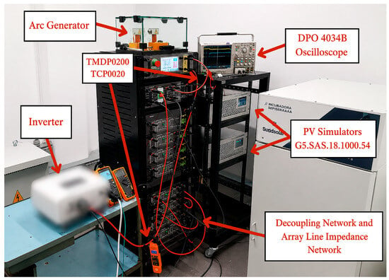
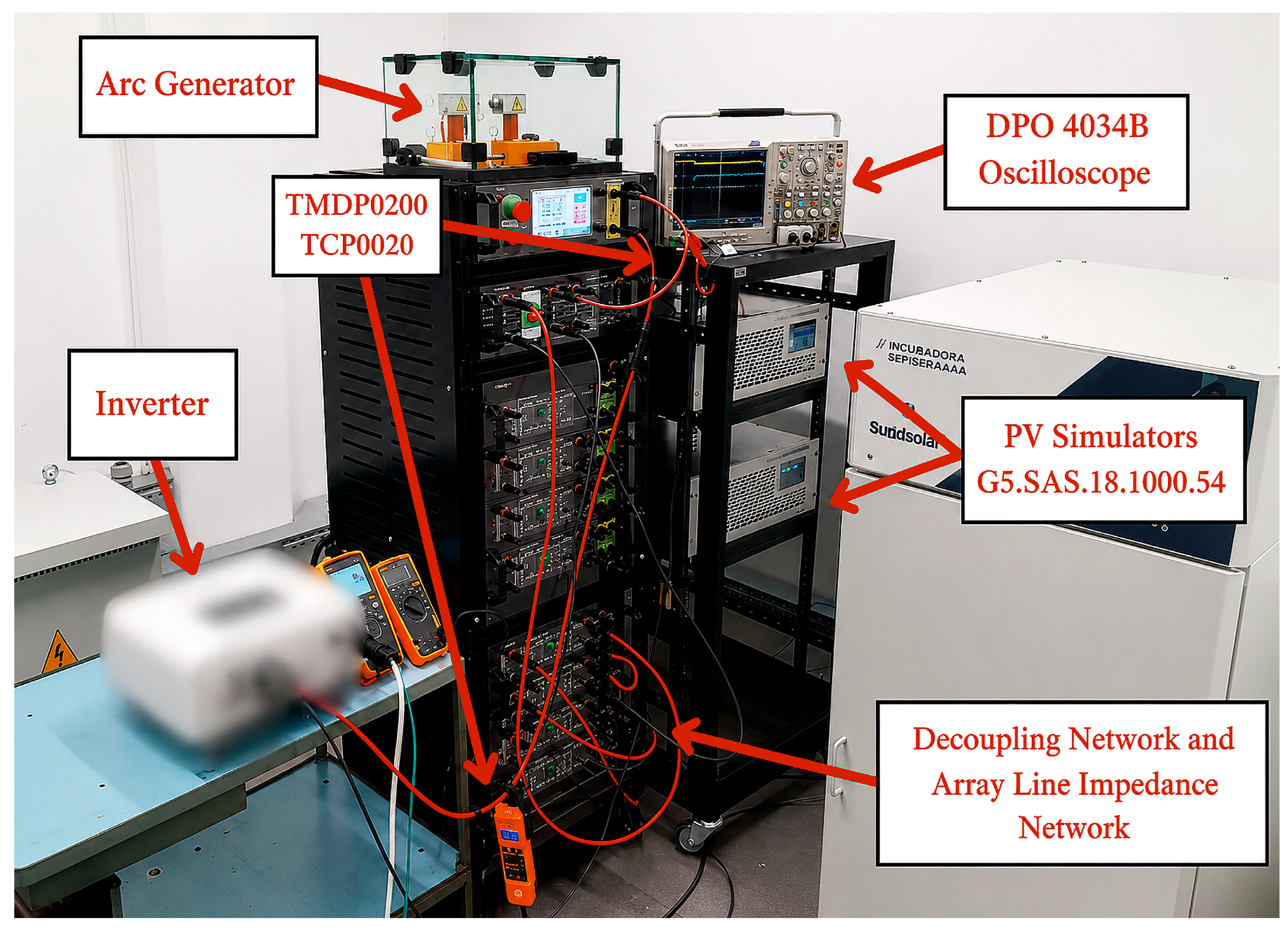
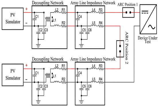
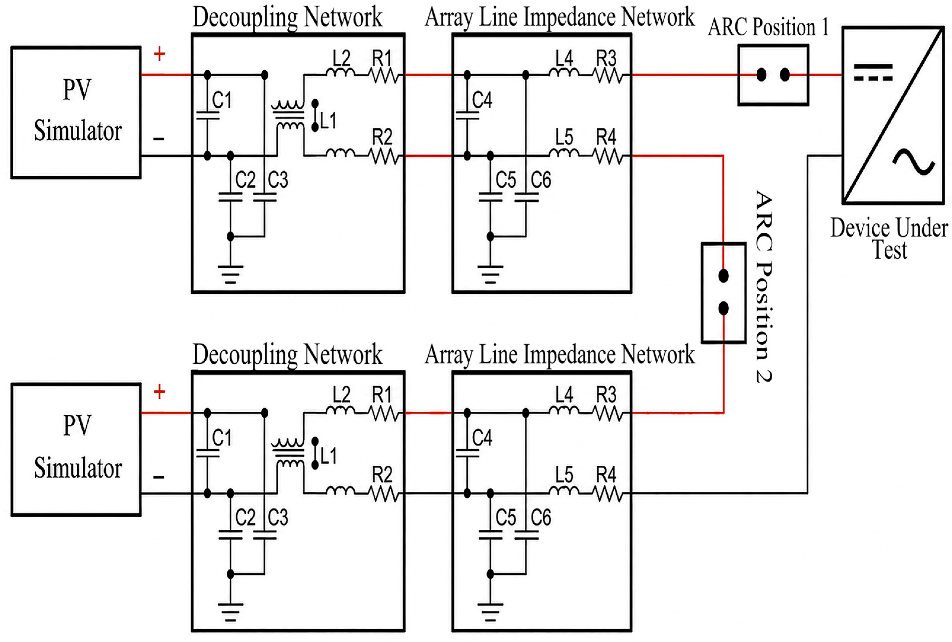
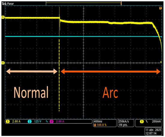
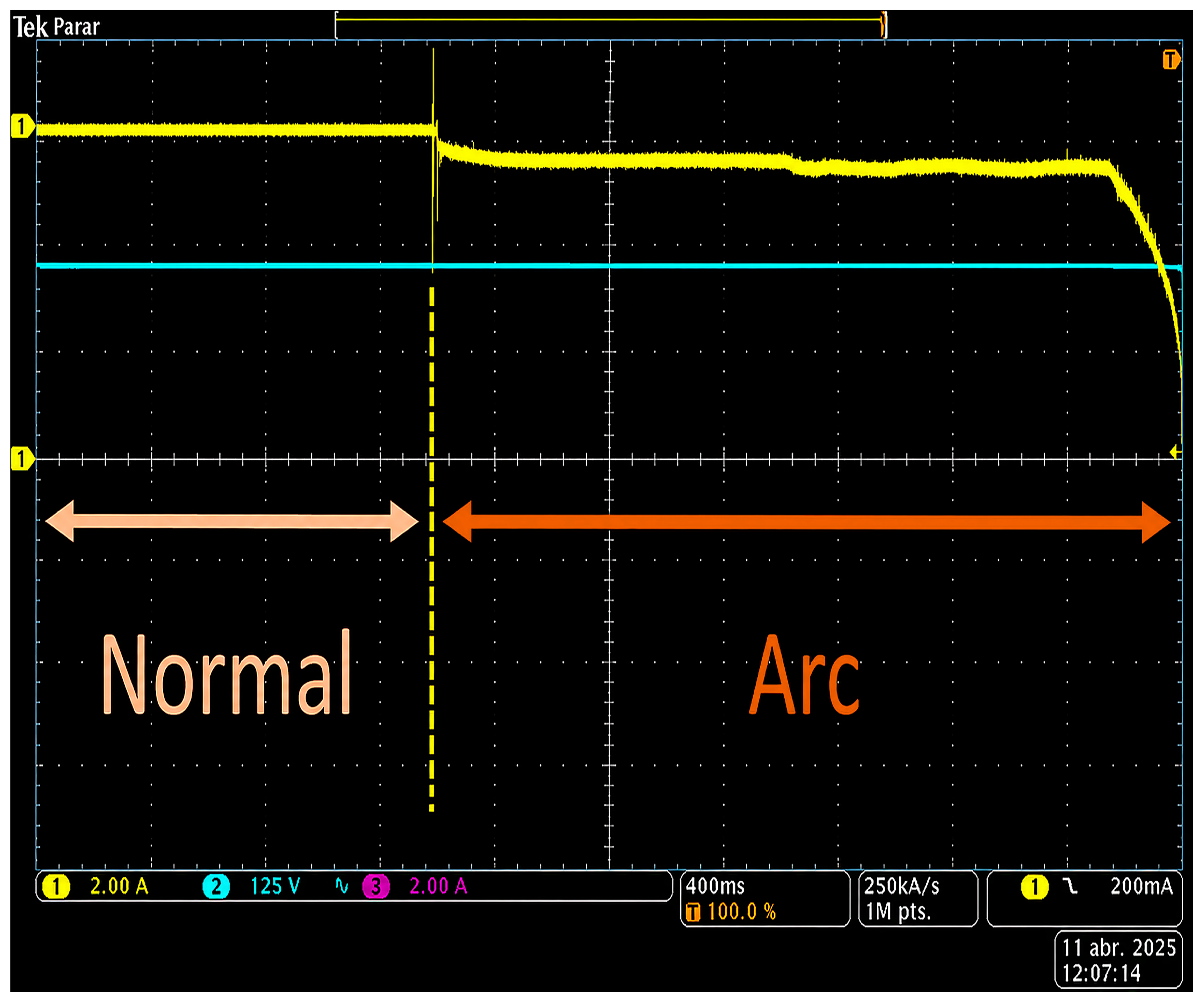
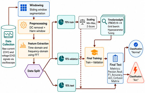
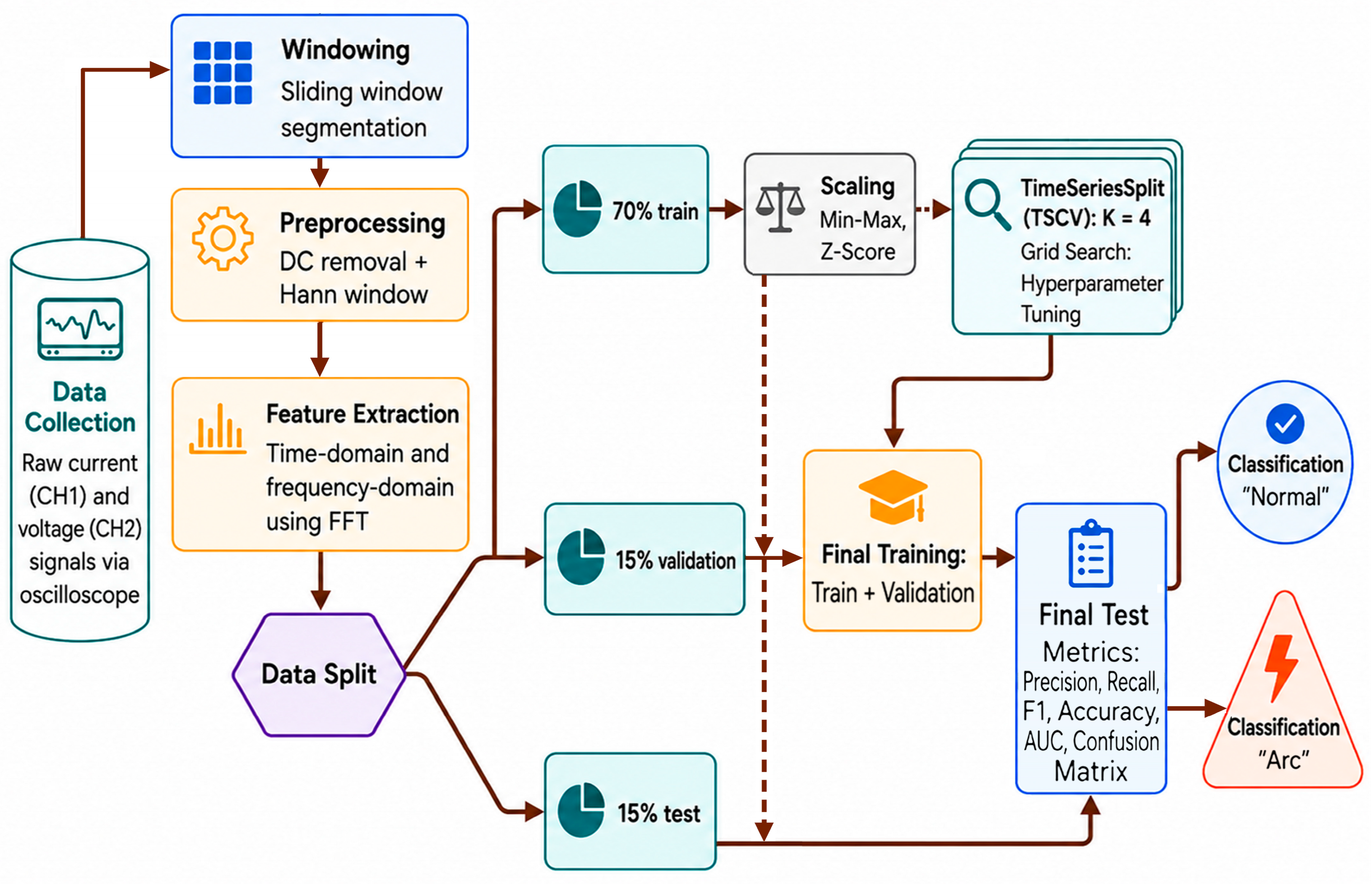
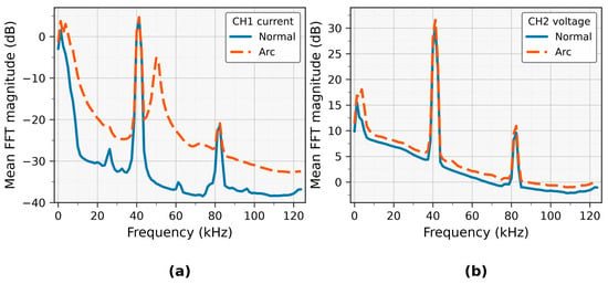
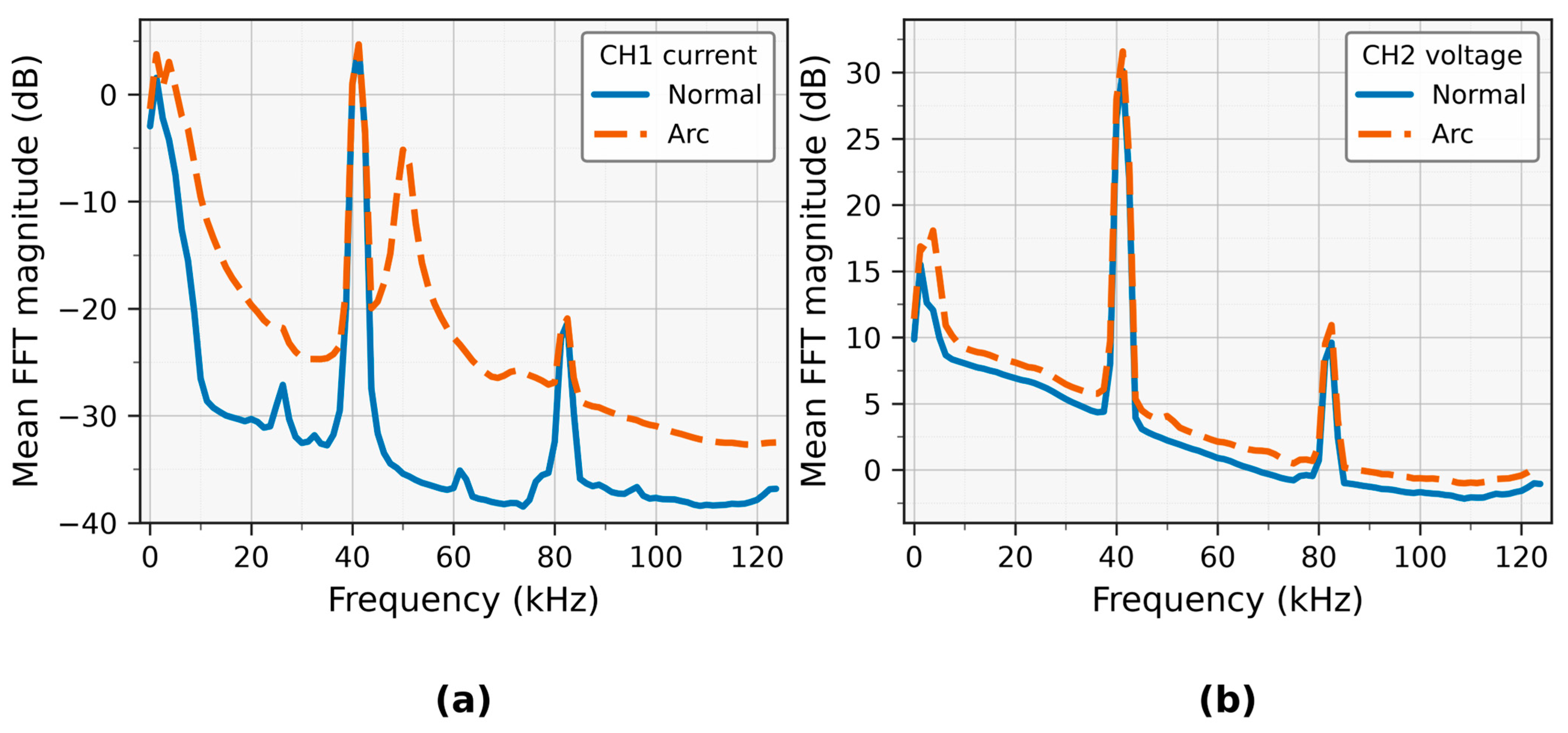
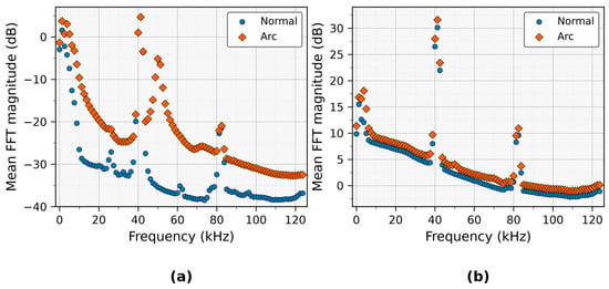
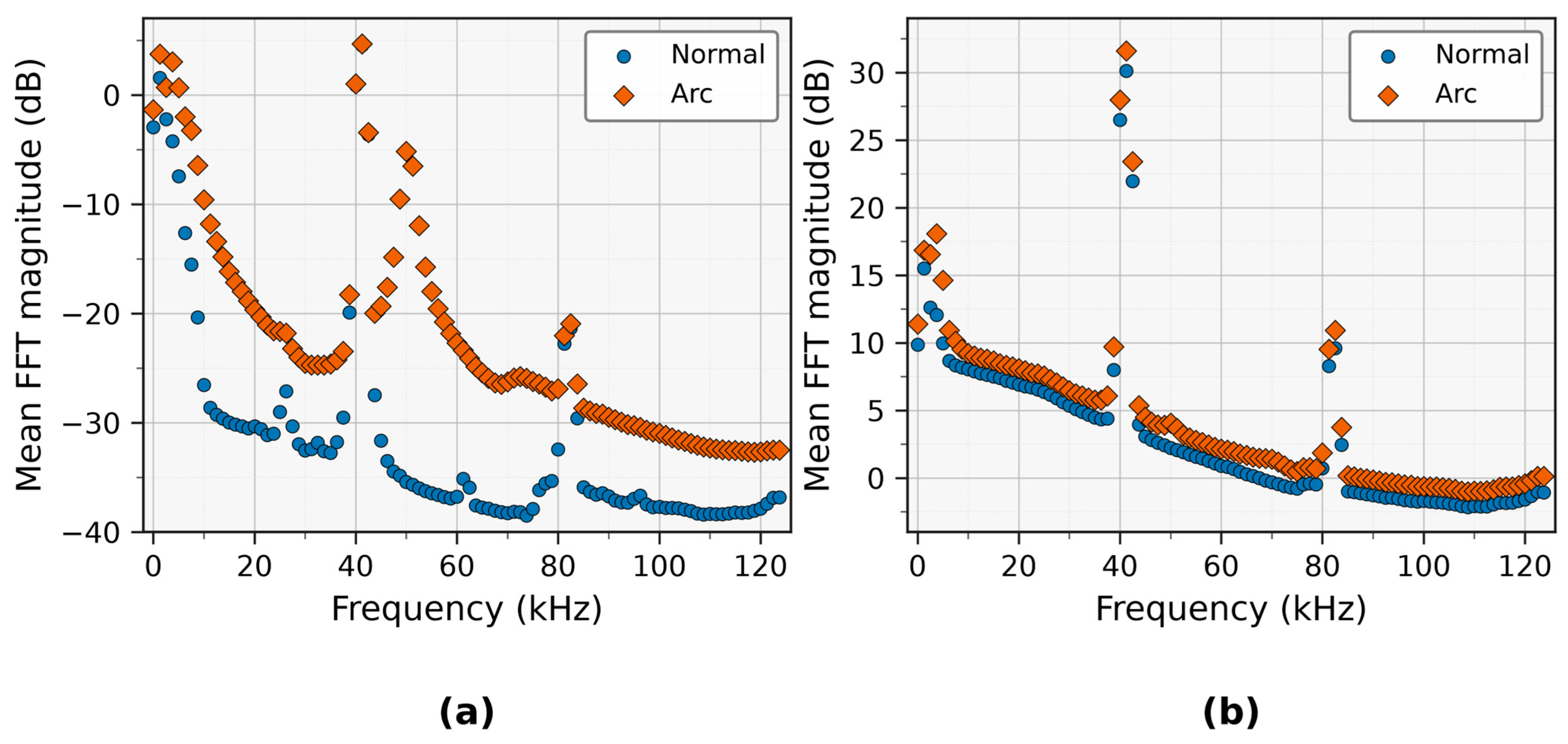
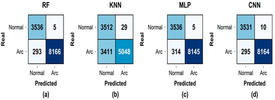
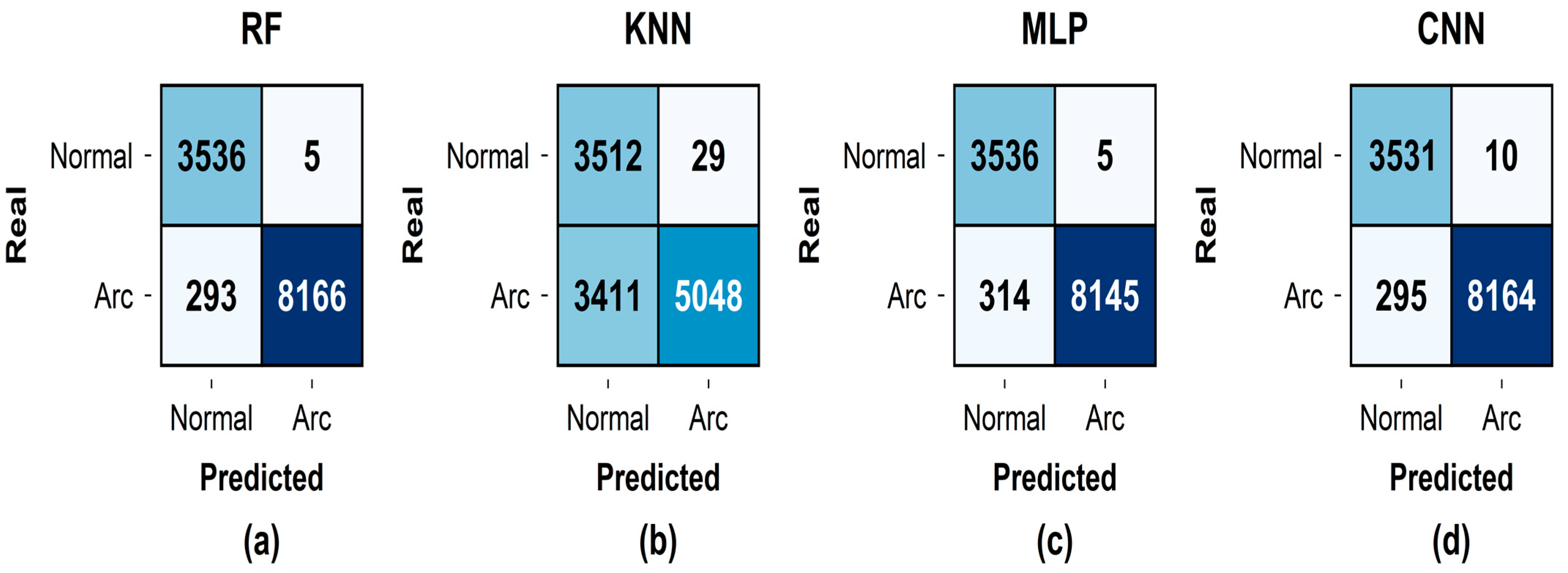
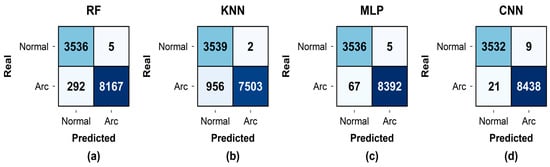
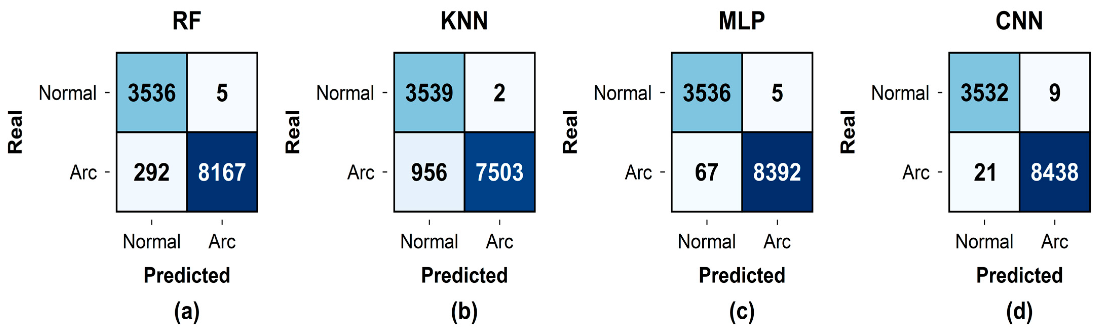
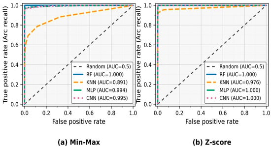
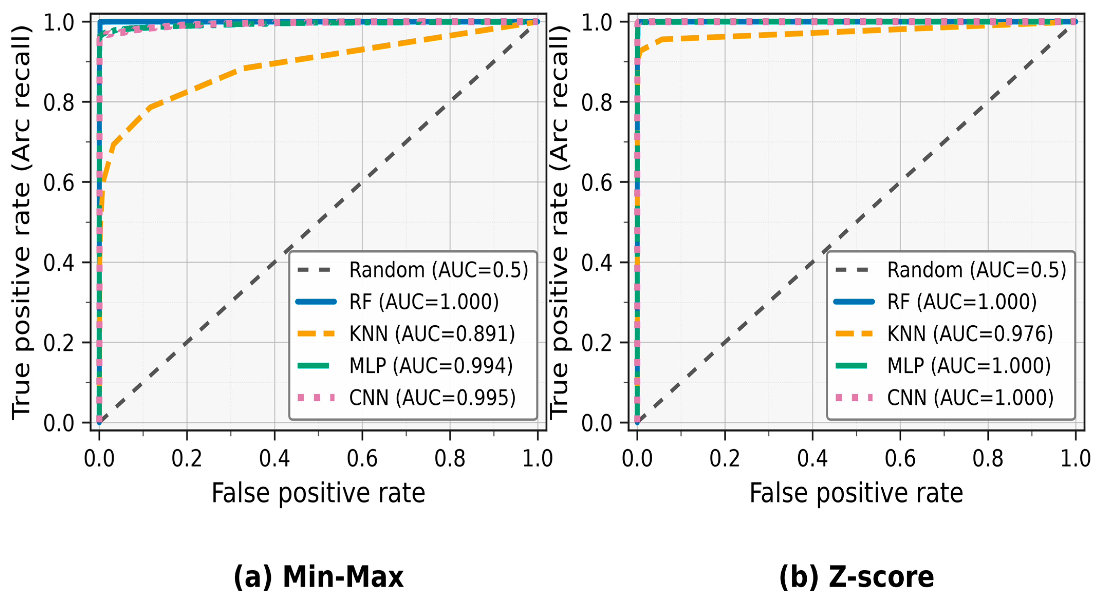
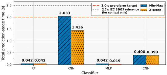
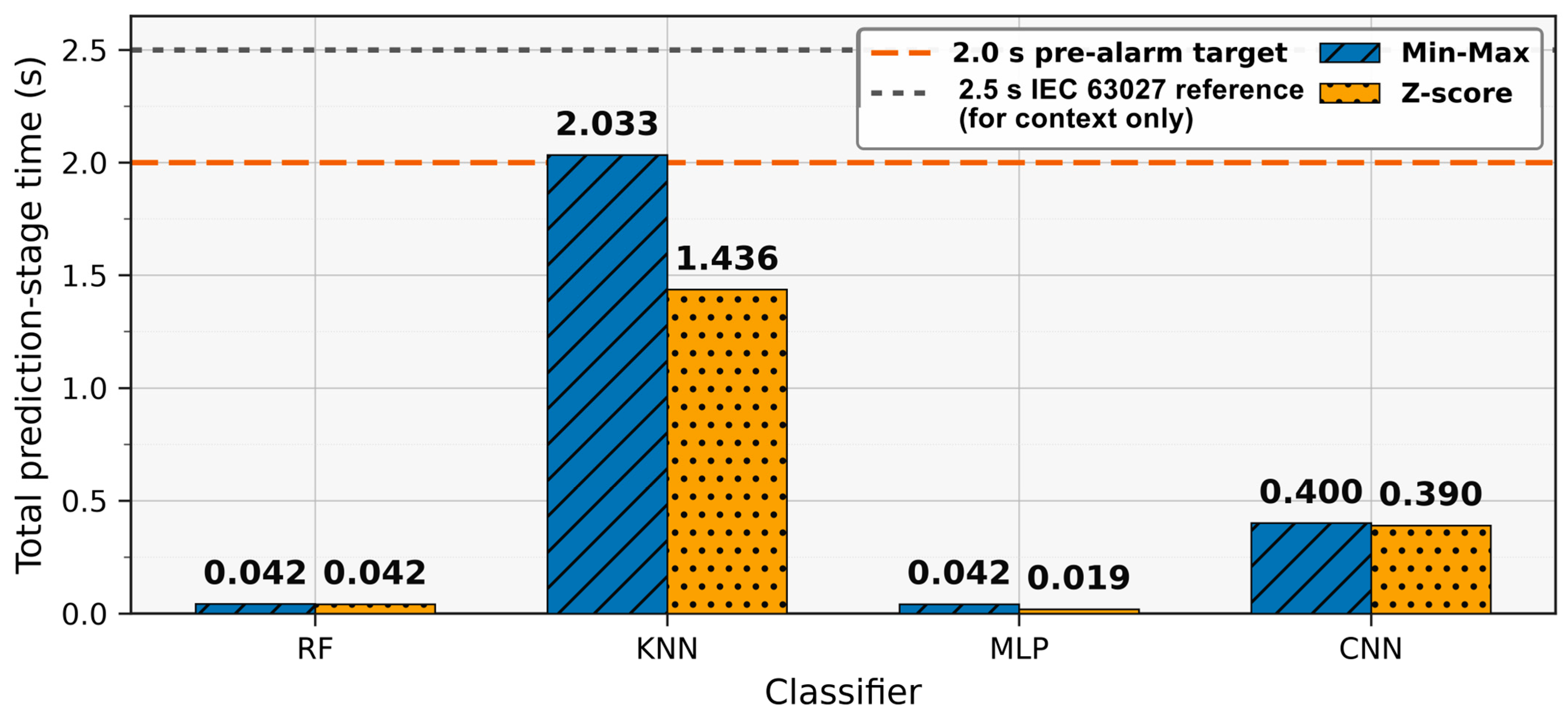

Disclaimer/Publisher’s Note: The statements, opinions and data contained in all publications are solely those of the individual author(s) and contributor(s) and not of MDPI and/or the editor(s). MDPI and/or the editor(s) disclaim responsibility for any injury to people or property resulting from any ideas, methods, instructions or products referred to in the content. |
© 2026 by the authors. Licensee MDPI, Basel, Switzerland. This article is an open access article distributed under the terms and conditions of the Creative Commons Attribution (CC BY) license.