


Abstract
High-resolution wind resource maps are essential for wind farm siting and renewable-energy planning, but national-scale assessment is often limited by sparse meteorological stations and the coarse resolution of reanalysis products. This study introduces a self-supervised Physics-Constrained Super-Resolution CNN (PC-SRCNN) that enhances ERA5 wind fields from 0.25° to 0.025°, for settings lacking a high-resolution, hourly-resolved reference wind field, by embedding kinematic and vertical-profile consistency as soft regularization penalties, without solving the full Navier-Stokes momentum balance. The framework was evaluated against 190 independent INMET stations, alongside interpolation, data-driven, and climatological baselines, using a station-wise bootstrap and the Diebold-Mariano test. The full model reduced the bootstrap MAE from 1.22 to 1.04 m/s relative to native ERA5, a 14.85% improvement confirmed by both tests, and achieved a vertical-profile of 0.90 against baselines below 0.70. Ablation shows physical regularization is not automatically beneficial: a variant constrained only by horizontal kinematics performed significantly worse than ERA5, with gains obtained only when vertical logarithmic-profile consistency was included. All other baselines evaluated were statistically indistinguishable from native ERA5 against station observations. These results indicate that sharper spatial detail alone is insufficient to improve wind-resource estimates unless supported by physically meaningful, vertically consistent constraints.
1. Introduction
Reliable wind-resource assessment requires spatially detailed wind information capable of supporting turbine siting, expected energy-yield estimation, investment screening, and grid-integration planning. Global reanalysis products such as ERA5 provide long-term and spatially continuous atmospheric fields, but their native resolution of 0.25° × 0.25°, approximately 27.83 km × 27.83 km per grid cell, is still too coarse for fine-scale wind-energy applications [1,2].
At this scale, relevant spatial controls on wind variability, including terrain gradients, surface roughness, coastal effects, vertical shear, and mesoscale flow structures, are averaged within coarse grid cells, reducing the reliability of direct reanalysis-based estimates for local wind-resource characterization [3,4].
This limitation is especially important in countries with large renewable-energy potential and uneven meteorological-station coverage, where high-resolution observations are not uniformly available for national-scale planning. Because wind-speed variability directly affects wind power output, capacity factors, and long-term generation and transmission expansion decisions, improving the spatial representation of wind fields is essential for robust renewable-energy planning and for climate-sensitive energy-system assessment [5].
Several approaches have been developed to reduce the resolution gap between coarse meteorological products and the spatial detail required by renewable-energy applications. Dynamical downscaling, usually based on regional atmospheric models such as Weather Research and Forecasting Model (WRF), provides physically consistent simulations and has been widely used for wind-resource assessment in complex terrain. However, its computational cost, sensitivity to boundary conditions and dependence on domain-specific configuration limit its scalability for repeated national-scale applications [6,7]. Statistical downscaling and interpolation-based methods offer computational efficiency, but their performance relies on the assumptions of spatial smoothness and stationarity, which may not always hold for wind fields influenced by terrain, coastal gradients and heterogeneous surface roughness [2,8,9].
Recently, deep learning has become an attractive approach to improve the representation of meteorological fields, as convolutional, generative, and operator-learning models can learn nonlinear spatial relationships that are difficult to learn using conventional statistical methods [3,10,11]. In renewable-energy studies, downscaling has also been applied to improve the temporal and spatial representation of climate inputs for energy-system modeling, especially in the solar-resource assessment, building-energy simulations, and grid-planning domains [12,13,14]. These studies demonstrate that coarse meteorological inputs can distort energy-system results, especially when local variability, ramping behavior, and resource intermittency are relevant to system design and operation.
For wind energy, recent super-resolution and terrain-aware machine-learning frameworks have shown that high-resolution wind fields can improve the representation of local variability and support more location-sensitive planning [2,3]. Nevertheless, important limitations remain. Some methods require high-resolution numerical simulations, CFD-generated training data, dense observational networks, or high-resolution reference fields that are not uniformly available across large territories. Others improve the visual or structural detail of wind maps but do not necessarily demonstrate statistically significant gains against independent in-situ observations. Therefore, there is still a need for a transferable framework that can refine coarse reanalysis wind fields using globally available inputs, while preserving physically meaningful atmospheric consistency and improving observational performance for wind-resource mapping.
High-resolution wind information is an important input for wind-energy planning because local wind variability directly affects turbine siting, expected energy yield, capacity-factor estimation, transmission planning, and investment-risk assessment [5,9,15,16,17,18,19,20,21,22,23,24]. Spatially explicit wind maps can aid planners in identifying technically feasible locations in light of environmental, social and infrastructure restrictions [25,26,27]. The availability of wind climatologies has been extended through global products like the Global Wind Atlas, which have been proven to be useful tools for initial resource screening and policy-oriented assessments [28]. Regional wind-resource assessments of this kind have been conducted worldwide, including recent work evaluating offshore wind potential along Saudi Arabia’s Red Sea coast using ERA5 reanalysis data combined with GIS-based site screening [29]. Nevertheless, datasets with a combination of spatial granularity, temporal homogeneity and observational dependability are needed for wind planning at the national level.
This issue is particularly relevant in Brazil due to its large onshore and offshore wind potential, but high-resolution wind observations are not uniformly distributed across the country. Earlier studies have pointed out the opportunities for wind energy development, along with restrictions on how much wind energy can be tapped due to incomplete spatial information, especially for offshore assessment, plant identification and national-scale planning applications [30,31].
Reanalysis products such as ERA5 provide spatially continuous and temporally consistent atmospheric fields [1,32], but their native grid resolution remains too coarse to resolve many local controls of wind variability. Terrain gradients, surface roughness, coastal transitions, vertical shear, and mesoscale circulation features may be smoothed within coarse grid cells, reducing their direct usefulness for fine-scale wind-resource assessment and engineering-oriented siting studies [3,4].
Different methodological families have been developed to bridge the gap between coarse atmospheric reanalysis and the spatial detail required for wind-resource assessment. Statistical downscaling and bias-correction methods estimate empirical relationships between coarse predictors and local observations or higher-resolution reference data. These approaches are computationally efficient and can correct systematic errors in mean values, variability, or probability distributions. However, their transferability depends on the availability and representativeness of calibration data, and bias correction alone does not create dynamically resolved subgrid wind structures.
Diagnostic microscale models such as WAsP and WindSim, explicitly account for local terrain and surface-roughness effects and are well established for site-specific wind-resource assessment. Nevertheless, they require detailed local information and are generally not designed to reconstruct temporally varying wind fields repeatedly over national-scale domains [33]. Dynamical downscaling with regional atmospheric models like the WRF offers a more physically complete alternative representation by solving atmospheric governing equations at finer resolution. This advantage is accompanied by substantial requirements for atmospheric boundary conditions, static geographical datasets, domain configuration, physical-parametrization selection, numerical spin-up, computational processing, and data storage, particularly for long hourly simulations over continental scale domains [6,7].
Machine-learning and deep-learning downscaling methods offer a more scalable alternative. Supervised super-resolution models generally learn mappings from paired coarse- and high-resolution wind fields generated from observations, WRF, CFD (Computational Fluid Dynamics), or other numerical simulations [34,35,36,37,38]. Terrain-aware models could use elevation, slope, aspect, land cover, surface roughness, or geographical coordinates as high-resolution predictors [3]. Their ability to reconstruct the fine-scale structure is therefore partly derived from high-resolution explanatory inputs or training targets that may not be consistently available in large data-limited regions [8]. Self-supervised and unsupervised approaches reduce dependence on paired targets, but their reconstructed spatial detail must still be evaluated against independent observations because agreement with the original coarse field does not demonstrate improved local accuracy [2,39,40,41,42].
The Global Wind Atlas (GWA) occupies a different methodological role [28]. It provides precomputed high-resolution climatological wind information derived through mesoscale and microscale modeling and is particularly valuable for preliminary wind-resource selection. However, it is principally a long-term climatological product rather than a framework for reconstructing the hourly temporal sequence of a selected ERA5 period. Consequently, direct GWA-based mapping and time-resolved ERA5 enhancement address related but distinct applications.
To address this gap, this study develops a self-supervised Physics-Constrained Super-Resolution Convolutional Neural Network (PC-SRCNN) for national-scale, time-resolved wind-resource mapping. The model improves the four ERA5 wind components at 10 and 100 m from 0.25° to 0.025° while preserving their coarse-scale consistency. Rather than learning from paired coarse and high-resolution wind fields, the network is optimized through a reconstruction loss and soft physical regularization based on horizontal kinematic coherence and logarithmic vertical-profile consistency.
The proposed framework differs from conventional statistical downscaling and bias correction because it does not estimate station-specific transfer functions or directly adjust an observed wind-speed distribution. It differs from supervised super-resolution and terrain-aware machine-learning models because no spatially complete high-resolution wind field is supplied as a training target, and the roughness-length layer is not used as a network predictor. Instead, roughness is introduced only through the vertical-profile loss, while the coarse-scale and horizontal-kinematic constraints are derived from the ERA5 fields being enhanced.
The framework also differs from WRF-based dynamical downscaling because it does not solve the atmospheric momentum, thermodynamic, and continuity equations or requires repeated numerical integration of a regional atmospheric model. It should therefore be interpreted as a computationally lightweight spatial-enhancement method rather than as a substitute for dynamical downscaling. Relative to direct Global Wind Atlas mapping, the framework reconstructs the hourly sequence associated with ERA5 rather than returning only a fixed long-term climatology. However, GWA climatologies are used indirectly to derive the static roughness-length layer, and therefore the method is not fully independent of atlas-derived information.
The principal methodological contribution is the combination of four elements: (i) self-supervised training without spatially complete high-resolution wind targets; (ii) simultaneous reconstruction of wind components at 10 and 100 m; (iii) physical regularization through both horizontal kinematic and vertical boundary-layer constraints; and (iv) independent station-based evaluation demonstrating whether the added fine-scale structure improves observational agreement. This final element is important because higher apparent resolution alone does not demonstrate improved wind-resource accuracy.
The model is applied to Brazil and validated against independent conventional meteorological stations, allowing the assessment of whether physically constrained super-resolution improves wind-resource estimates beyond native reanalysis and purely data-driven baselines.
2. Methodology
In this study, a PC-SRCNN framework is developed to enhance the spatial resolution of wind speed fields over Brazil. The model uses hourly eastward and northward wind components at 10m and 100 m above ground level as input a variable, with the objective of increasing the nominal spatial resolution from 0.25° to 0.025° while preserving large-scale statistical consistency and physically plausible spatial structures.
ERA5 hourly data on single levels, available from 1940 to the present, was used as the primary source of reanalysis wind information [1]. Complementary wind speed fields at 10m and 100m from the Global Wind Atlas were used to derive a spatially distributed roughness-length layer over Brazilian territory [28]. Observational wind-speed records from conventional meteorological stations operated by the Brazilian National Institute of Meteorology (INMET) for January 2024 were used to evaluate the model performance against the independent in-situ measurements [43].
The methodological framework is organized into three main stages.
- First Step: ERA5 wind fields are used to construct a self-supervised super-resolution framework, where degraded low-resolution inputs are mapped to reference-resolution fields. The PC-SRCNN loss function includes kinematic and vertical-profile regularization terms to promote physically plausible reconstructions without solving the full Navier–Stokes system.
- Second Step: The neural-network architecture and loss-weighting parameters are tuned through Bayesian optimization, allowing systematic exploration of hyperparameter configurations and selection of a model that balances reconstruction accuracy, physical regularization, and computational efficiency.
- Third Step: The optimized model is evaluated using ERA5-derived reconstruction metrics and independent wind-speed observations from INMET stations. Model performance is assessed through conventional error metrics, spatial cross-validation, bootstrap confidence intervals, and statistical tests against reference approaches. This validation strategy quantifies the accuracy, robustness, and physical consistency of the proposed PC-SRCNN framework, supporting its application to wind-resource assessment and spatial energy-planning studies.
2.1. Wind-Field Database and Geospatial Preprocessing
ERA5 hourly single-level reanalysis data were used as the primary source of wind-field information [1]. The variables extracted were the eastward (u) and northward (v) wind components at 10 m and 100 m above ground level. ERA5 provides these fields at a native spatial resolution of 0.25° × 0.25°, corresponding to approximately 27.83 km × 27.83 km per grid cell. The analysis was restricted to Brazilian territory, bounded by 6° N–33° S and 35° W–74° W.
The extracted ERA5 fields were converted into gridded tensors containing latitude, longitude, time, and the four wind components (, , , and ). Wind-speed magnitudes at 10 m and 100 m were then computed as
These magnitudes were used for exploratory diagnostics, comparison with station observations, and evaluation of vertical wind-speed consistency.
Complementary wind-speed climatologies at 10 m and 100 m from the Global Wind Atlas were used to derive a spatially distributed roughness-length layer over Brazil [28]. This layer provides an auxiliary geospatial descriptor of surface–atmosphere interaction and supports the logarithmic wind-profile constraint used in the PC-SRCNN framework.
The ERA5 fields were organized into training, validation, and testing subsets. The training subset was used to fit the super-resolution mapping between degraded low-resolution inputs and reference-resolution ERA5 fields. Validation samples were used for hyperparameter selection and loss-weight calibration, whereas the test subset was reserved for independent model evaluation. Conventional meteorological-station records from the Brazilian National Institute of Meteorology (INMET) were used as independent in-situ observations to assess model performance against ground measurements [43]. The features from ERA5 fields used to build the training, validation, and testing sets are described in Table 1.
Table 1.
ERA5 reanalysis variables used for wind field characterization and model development over Brazilian territory.
Before model training, all wind components were clipped to the Brazilian domain, checked for missing values, aligned on a common latitude–longitude grid, and normalized using statistics computed from the training subset. The same preprocessing parameters were applied to validation and test data to avoid information leakage. The resulting geospatial database supports the comparison between native ERA5, purely data-driven super-resolution, and physics-constrained reconstructions.
Exploratory diagnostics of the ERA5 wind-field variables, including distributional analysis, descriptive statistics, and correlation structure, are provided in Appendix A.1. These analyses confirm the non-Gaussian nature of the wind components and the strong vertical coherence between 10 m and 100 m fields, providing empirical motivation for the vertical-profile consistency constraint used in the PC-SRCNN loss function.
2.2. Roughness Map
To derive the roughness-length map for Brazilian territory, historical mean wind-speed maps at 10 m and 100 m above ground level were obtained from the Global Wind Atlas [44]. These two input layers, shown in Figure 1a,b, provide spatially distributed estimates of wind-speed conditions at 10 m and 100 m above ground level over Brazil. The roughness length was then estimated independently for each pixel by inverting the logarithmic wind-profile relationship between the 10 m and 100 m wind speeds.
Figure 1.
Historical mean wind speed maps over Brazilian territory (author-generated visualization from Global Wind Atlas data) at (a) 10 m and (b) 100 m above ground level. The maps were aggregated from the native 250 m resolution to 0.025° using bicubic interpolation for compatibility with the model framework. Units: m/s.
The logarithmic wind profile is derived from surface-layer similarity theory [45] and is widely used in boundary-layer meteorology [46,47] and wind-resource assessment [48]. In this study, the formulation was used to describe the vertical variation of wind speed as a function of height and surface roughness.
Given the wind speeds at 10 m and 100 m, the roughness length was computed pixel by pixel, allowing the construction of a spatially distributed roughness map compatible with the PC-SRCNN framework. The formulation is expressed as follows:
where and denote the historical mean wind-speed magnitudes at 10 m and 100 m, respectively.
This formulation assumes neutral atmospheric stability [45]. Consequently, vertical-profile loss constrains reconstructed 10 and 100 m wind speeds toward a neutral logarithmic relationship, even when the actual atmospheric surface layer is stable or unstable. Under stable stratification, which frequently occurs during nighttime conditions, suppressed turbulent mixing generally produces stronger vertical wind shear than predicted by the neutral profile.
For a given reconstructed wind speed at 10 m, the neutral formulation may therefore underestimate the corresponding wind speed at 100 m and may penalize physically valid stable profiles. Under unstable or convective conditions, enhanced turbulent mixing produces a flatter vertical profile; the neutral formulation may consequently overestimate the 100 m wind speed inferred from the 10 m field and constrain the model toward excessive vertical shear [46,47].
This limitation is particularly relevant in tropical regions, where strong daytime convection and pronounced diurnal changes in surface-layer stability are common. Because the present formulation does not include time-varying stability information, the effect of may differ between daytime convective periods and nighttime stable periods. Some errors may partially offset when aggregated over time, but the model may still exhibit stability-dependent biases at individual hours. The present validation does not stratify the results by atmospheric-stability class; therefore, the magnitude of these effects cannot be quantified from the current analysis.
In coastal regions, the diurnal land–sea-breeze cycle, changes in surface roughness across the coastline, and the development of internal boundary layers violate the assumptions of stationary, horizontally homogeneous surface-layer flow underlying the logarithmic profile. The resulting error may depend on wind direction, upstream fetch, coastline geometry, and time of day, potentially increasing both the dispersion and local bias of the reconstructed wind speeds.
In complex terrain, flow acceleration over ridges, sheltering, channeling, separation, and terrain-induced pressure gradients similarly violate the one-dimensional and horizontally homogeneous assumptions of the logarithmic formulation. The neutral-profile constraint should therefore be interpreted as a soft regularizer that promotes approximate vertical coherence rather than as a complete representation of boundary-layer flow under all atmospheric and topographic conditions.
Because the Global Wind Atlas provides wind-speed fields at a native spatial resolution of 250 m (0.0025°), the 10 m and 100 m layers were resampled to the 0.025° model grid used in the PC-SRCNN framework. This preprocessing step was performed using bicubic interpolation to obtain smooth spatial transitions while preserving broad local gradients in the wind-speed fields. The roughness-length map was then computed pixel by pixel using Equation (2) and the resampled 10 m and 100 m wind-speed fields shown in Figure 1, with the final result presented in Figure 2.
Figure 2.
Roughness-length map over Brazilian territory (author-generated visualization derived from Global Wind Atlas source data), obtained from historical mean wind speed data at 10 m and 100 m above ground level (Figure 1) using the logarithmic wind-profile inversion defined in Equation (2). Source data: Global Wind Atlas [44].
The roughness-length field used in the vertical-profile constraint is not obtained from direct surface measurements. It is derived by inverting the neutral logarithmic wind-profile relationship using climatological wind-speed fields at 10 and 100 m from the Global Wind Atlas (GWA) [28]. Consequently, uncertainty in GWA wind climatologies, their underlying mesoscale and microscale modeling chain, the spatial resampling procedure, and the logarithmic-profile inversion are propagated into the estimated field .
This introduces a degree of methodological dependence between the proposed framework and an external model-derived wind product. The dependence is indirect rather than equivalent to training against GWA: the GWA wind fields are not used as time-varying network inputs or high-resolution prediction targets, but only to derive the static roughness field entering the vertical-profile loss. Nevertheless, spatial structures or biases contained in the GWA climatology may influence the expected relationship between reconstructed wind speeds at 10 and 100 m and may therefore be partially transferred to the PC-SRCNN output through .
Additional uncertainty arises because is inferred under neutral atmospheric stability and is treated as temporally invariant. The resulting field does not represent changes in effective aerodynamic roughness associated with seasonal vegetation dynamics, land-use change, soil moisture, atmospheric stability, wind direction, or heterogeneous upstream fetch. Moreover, the logarithmic inversion may produce unrealistic or highly sensitive estimates where the difference between the GWA wind speeds at 10 and 100 m is small or inconsistent with the assumed profile. Although numerical bounds and preprocessing can limit extreme values, they do not remove the underlying structural uncertainty.
The GWA-derived roughness field should therefore be interpreted as a model-based regularization proxy rather than as an independently observed surface property. Future work should assess the sensitivity of the results to alternative roughness sources, including satellite-derived land-cover products, land-use-to-roughness lookup tables, ERA5 surface parameters, or directly measured site information, and should quantify how uncertainty in propagates into the reconstructed wind fields.
2.2.1. Super-Resolution Convolutional Neural Network
Super-Resolution Convolutional Neural Networks (SRCNNs) are deep learning models designed to reconstruct finer spatial representations from coarse-resolution inputs [49,50,51,52,53,54,55,56,57,58]. In this study, the SRCNN formulation was adapted to gridded wind fields, where the objective is to learn a nonlinear mapping from coarse ERA5 wind components to a refined spatial representation suitable for wind-resource mapping.
Let denote the low-resolution input field, where H and W are the spatial dimensions and C is the number of input channels. In this application, the channels correspond to the ERA5 wind components , , , and . The super-resolved output is represented by , where r denotes the spatial upscaling factor applied to the horizontal dimensions of the input field. The SRCNN then learns a nonlinear mapping from the low-resolution input to the corresponding super-resolved representation.
where represents the convolutional neural network and denotes its trainable parameters.
Unlike conventional supervised image super-resolution, no independent high-resolution wind-field observations are available over the full Brazilian domain on an hourly basis. Therefore, the SRCNN was trained in a self-supervised setting. The coarse ERA5 fields provide the large-scale reference, while the network output is evaluated by comparing its downsampled representation with the original ERA5 input. This strategy allows the model to learn spatial refinement patterns without requiring external high-resolution ground-truth fields.
The reconstruction objective is formulated as a coarse-scale consistency loss:
where is obtained by applying a downsampling operator that maps the super-resolved output back to the native ERA5 grid. This loss constrains the reconstructed field to remain consistent with the original coarse-resolution reanalysis while allowing the model to introduce finer spatial structure at the target resolution.
The SRCNN architecture follows three main steps. First, the low-resolution wind field is interpolated to the target grid using bicubic interpolation, providing an initial smooth estimate of the high-resolution domain. Second, the interpolated field is passed through convolutional layers with nonlinear activation functions, which extract hierarchical spatial features and refine local gradients. Finally, the output layer reconstructs the super-resolved wind components without applying an additional activation function, preserving the continuous nature of wind-speed fields.
Although this purely data-driven SRCNN can enhance spatial detail, it does not explicitly enforce atmospheric consistency. In environmental applications, this may lead to fields that are visually sharper but physically inconsistent or not more accurate against independent observations. For this reason, the SRCNN is used as the data-driven baseline, while the proposed PC-SRCNN extends this formulation by adding kinematic and vertical-profile constraints to the loss function.
2.2.2. PC-SRCNN: Physics-Constrained Super-Resolution
The PC-SRCNN extends the SRCNN backbone by embedding physical information through soft regularization terms added to the training objective, rather than by explicitly solving the full Navier–Stokes momentum equations [59,60,61]. The framework enhances coarse ERA5 wind fields from 0.25° to 0.025° while preserving large-scale consistency and physically plausible spatial structures.
The complete PC-SRCNN workflow is illustrated in Figure 3. The SRCNN backbone maps low-resolution wind fields to super-resolved outputs, while three complementary loss components guide the optimization toward physically coherent reconstructions.
Figure 3.
Schematic of the PC-SRCNN framework integrating data-driven super-resolution with horizontal kinematic and vertical-profile regularization. The SRCNN backbone maps coarse wind fields to super-resolved outputs, while the loss function penalizes deviations from coarse-scale consistency, horizontal kinematic coherence, and logarithmic vertical-profile consistency.
The three loss components serve distinct purposes:
- Coarse-scale consistency loss (): Preserves consistency between the super-resolved output and the original ERA5 field at the native coarse scale, ensuring that large-scale flow patterns are maintained.
- Horizontal kinematic regularization (): Penalizes unrealistic divergence and rotational artifacts in the reconstructed wind components, promoting spatially coherent horizontal structures.
- Vertical logarithmic-profile consistency (): Enforces consistency between 10 m and 100 m wind speeds using the logarithmic wind-profile relationship, anchoring the reconstruction to boundary-layer physics.
Each loss component is detailed in the following subsections.
2.2.3. Coarse-Scale Consistency Loss ()
The coarse-scale consistency loss constrains the super-resolved output to remain consistent with the original ERA5 input when mapped back to the native coarse grid. This loss is identical to the SRCNN reconstruction objective defined in Equation (4) and serves the same purpose in the PC-SRCNN framework: ensuring that the introduction of physical constraints does not compromise the statistical consistency of the wind fields.
Let denote the low-resolution ERA5 input and the super-resolved prediction, where r is the spatial upscaling factor. A reconstructed coarse field is obtained by applying a downsampling operator to the super-resolved output, as shown in Equation (5):
The downsampling operator is implemented as spatial average pooling over non-overlapping blocks, consistent with the spatial upscaling factor r applied by the network. Each block of pixels in the super-resolved field is averaged to produce a single pixel at the native ERA5 resolution.
The coarse-scale consistency loss is then defined as Equation (6):
where N denotes the number of training samples. This term discourages artificial fine-scale structures that are inconsistent with the large-scale reanalysis signal and helps preserve the mean flow patterns represented by ERA5. Without this constraint, the physical regularization terms could drive the reconstruction away from the reanalysis baseline, producing fields that are physically plausible but statistically inconsistent with the observed large-scale circulation. Without this term, the physical constraints could drive the reconstruction away from the large-scale reanalysis signal, compromising the statistical consistency of the wind fields.
2.2.4. Horizontal Kinematic Regularization Loss ()
Horizontal kinematic consistency was introduced by penalizing unrealistic spatial behavior in the reconstructed wind components. Let and denote the reconstructed eastward and northward wind components at a given height. A horizontal divergence residual is defined as
which discourages artificial convergence or divergence patterns introduced during super-resolution.
A rotational residual is also computed as
This term provides a diagnostic of local horizontal rotation in the reconstructed field. In this implementation, it is used as a regularization term to control excessive small-scale rotational artifacts introduced by the neural network.
Physically, approximates the horizontal divergence of the reconstructed wind field, whereas approximates the vertical component of relative vorticity. Horizontal divergence represents local horizontal expansion or contraction of the flow and may be associated with processes such as frontal convergence, terrain-induced lifting, convection, or compensating vertical motion. Relative vorticity represents local horizontal rotation. Both quantities are physically nonzero in real atmospheric flows; therefore, the present terms do not constitute exact conservation equations.
In the implemented formulation, the squared magnitudes of divergence and vorticity are used as soft smoothness priors. Their purpose is to discourage the network from generating excessively strong small-scale convergence, divergence, or rotation during super-resolution. Because the loss penalizes the absolute derivative magnitudes rather than their departure from a coarse-resolution reference, it may also suppress physically meaningful structures. The regularizer should therefore be interpreted as a kinematic artifact-control term rather than as enforcement of horizontal mass conservation or preservation of the complete atmospheric vorticity field.
Spatial derivatives were approximated numerically using Sobel finite-difference kernels:
For any reconstructed field , the horizontal gradients are approximated as
These derivatives are computed in grid pixel units, not physical distance. Since the Brazilian domain spans a wide range of latitudes (6° N–33° S), the physical distance represented by one pixel is not constant, varying with latitude in the zonal direction as grid spacing in meters scales with the cosine of latitude. Both derivatives are therefore divided by the corresponding grid spacing in meters, constant in the meridional direction and latitude-dependent in the zonal direction, computed once from the domain’s fixed geometry and not supplied to the network as an explicit coordinate input. This preserves the correct physical units and interpretation of the residuals.
Where ∗ denotes convolution. The horizontal kinematic regularization loss is defined as
where N is the number of spatial grid points. This loss does not impose the full Navier–Stokes momentum balance; instead, it acts as a soft kinematic regularizer that promotes spatially coherent wind reconstructions.
2.2.5. Vertical Logarithmic-Profile Consistency Loss ()
Vertical consistency between the 10 m and 100 m wind fields was promoted using the logarithmic wind-profile relationship. Under neutral atmospheric stability, the mean horizontal wind speed at height z can be written as
where is the friction velocity, is the von Kármán constant, and is the roughness length.
Using the 10 m wind speed as a reference, this expression can be written in normalized form as
The logarithmic wind profile enables vertical extrapolation of near-surface winds to higher altitudes. Using the reconstructed 10 m wind field as a reference, we project the wind speed to 100 m and compare it with the model’s direct reconstruction at that height.
Let denote the reconstructed horizontal wind velocity at 10 m, and the reconstructed velocity at 100 m. The projected velocity at 100 m, , is obtained from the logarithmic profile as:
Consistency between predicted and physically projected velocities is promoted through the vertical projection loss , defined as the mean squared deviation between both fields over all spatial grid points :
where N is the number of spatial grid points. This term promotes consistency between the directly reconstructed 100 m wind-speed field and the 100 m field implied by the reconstructed 10 m wind speed and the roughness-length map.
2.2.6. Composite Training Objective
The final PC-SRCNN objective combines coarse-scale consistency, horizontal kinematic regularization, and vertical logarithmic-profile consistency:
where , , and are positive weighting coefficients controlling the contribution of each loss component. These coefficients were selected through Bayesian optimization, allowing the model to balance reconstruction fidelity, spatial coherence, and vertical physical consistency.
2.3. Hyperparameter Optimization and Validation Strategy
Bayesian optimization was used to tune the architectural and loss-weighting hyperparameters of each model using the Keras Tuner framework [62]. The search was conducted over 50 trials, including 15 randomly initialized configurations. Each candidate model was trained for up to 50 epochs with a batch size of 8, using early stopping with a patience of 17 epochs. The learning rate was reduced by a factor of 0.95 when no improvement was observed for 15 consecutive epochs.
The optimized hyperparameters included the activation function, learning rate, physical-loss weighting coefficients, number of convolutional layers, number of filters, and kernel sizes. For the U-Net baseline, the search space included the base number of filters, network depth, number of convolutions per block, and final kernel size. The full hyperparameter search space and the Bayesian optimization formulation are provided in Appendix A.2.
Each candidate configuration was ranked using a spatial cross-validation criterion computed over nine held-out regions. For each fold, the validation objective combined coarse-scale consistency, horizontal kinematic regularization, vertical-profile consistency, and an observational agreement term:
where denotes the set of valid stations at the current time step (those with non-missing measurements and wind speed above 0.1 m/s), are the grid indices of station s, and is the corresponding observed wind speed.
The term , shown in Equation (18), measures the agreement between predicted 10 m wind-speed magnitude and independent INMET station observations within the held-out validation region. This term was used only for hyperparameter ranking and was never backpropagated through the neural-network weights. Therefore, the models were trained exclusively on ERA5-derived loss components, while station observations entered the pipeline only through model selection and final independent validation.
The use of INMET observations was separated between hyperparameter selection and final evaluation primarily in the temporal dimension. During Bayesian optimization, station observations from a single hourly snapshot were included in to rank candidate hyperparameter configurations. These observations were not backpropagated through the neural-network weights; model training remained based exclusively on the ERA5-derived coarse-scale and physical-loss components. The hourly snapshot used for hyperparameter ranking was excluded from the subsequent station-based evaluation, so no station observation at the same timestamp was used in both model selection and final performance assessment.
The spatial cross-validation procedure provided an additional assessment of geographical robustness, but it did not create complete station-level independence between model selection and final evaluation. In each leave-one-region-out fold, the INMET observations located in the held-out region were used to evaluate candidate configurations through . Because the ranking criterion was averaged across all nine folds, the complete network of 190 stations contributed collectively to the selection of the final hyperparameter configuration. The same stations were subsequently used for final evaluation at temporally held-out hours.
Accordingly, the final station-based assessment should be interpreted as a temporally out-of-sample evaluation rather than a fully independent spatial validation. It tests whether a configuration selected using one hourly station snapshot generalizes to additional hours at the same observational network. A stricter assessment of spatial transferability would require reserving a subset of stations or geographical regions exclusively for final testing, without using them for training, hyperparameter selection, or loss-weight calibration.
Deploying this framework in a different region would accordingly require repeating this hyperparameter selection process using that region’s own observational network, rather than transferring the hyperparameters selected here directly.
Model performance was assessed using two complementary validation strategies. First, coarse-scale reconstruction fidelity was evaluated by comparing the downsampled super-resolved outputs with the native ERA5 fields using MAE, RMSE, MSE, , SMAPE, and MAPE. These metrics quantify whether each model preserves the large-scale reanalysis signal, but they do not by themselves demonstrate superior observational skill. Statistical equivalence with the ERA5 reference fields was additionally assessed using Two One-Sided Tests (TOST), as detailed in Appendix A.2.
Second, and most importantly, observational performance was evaluated against independent hourly measurements from INMET conventional meteorological stations. Because hourly observations from the same station are serially dependent and prediction errors are spatially clustered by station, uncertainty was evaluated using two complementary procedures. First, non-parametric confidence intervals for MAE were calculated through station-wise cluster resampling. Entire stations, rather than individual station–hour observations, were sampled with replacement in each of B = 10,000 bootstrap repetitions. All hourly observations associated with a selected station were retained, preserving within-station temporal dependence and the paired error structure between each model and native ERA5.
Statistical differences between each model and ERA5 were additionally assessed using the Diebold–Mariano test [63,64]. To avoid treating station–hour observations as mutually independent, the loss differential was first calculated at each station and hour and then averaged across all valid stations for each hour:
where is the absolute-error loss and is the number of valid stations at hour t. Negative values of indicate a lower average loss for the evaluated model than for ERA5. The DM statistic was computed from the temporal sequence , with its long-run variance estimated using a heteroskedasticity- and autocorrelation-consistent Newey–West estimator. This correction accounts for serial dependence in the hourly loss differential.
As a complementary inference procedure, a paired station-wise bootstrap significance test was applied. For each resample, the MAE difference relative to ERA5 was calculated as
Therefore:
A model was considered significantly different from ERA5 when the 95% bootstrap confidence interval for excluded zero. Negative values of indicate improvement over ERA5. The DM test therefore evaluates temporal persistence in the national mean loss differential, whereas the station-wise bootstrap evaluates robustness to the spatial composition of the observational network.
2.4. Spatial Cross-Validation
Spatial cross-validation was implemented by partitioning the Brazilian domain into nine regions, as illustrated in Figure 4. A leave-one-region-out procedure was adopted: in each iteration, eight regions were used for training and the remaining region was reserved for validation. This process was repeated until each region had served once as the held-out validation domain. The procedure reduces the influence of spatial autocorrelation and provides a more stringent assessment of model generalization across geographically distinct areas.
Figure 4.
Partition of the Brazilian domain into nine regions used for spatial cross-validation.
During each cross-validation iteration, each model was trained using only the loss components consistent with its theoretical design, as summarized in Table 2. Specifically, was applied to models without physical constraints, to the physics-constrained variant, and to the complete proposed framework. This configuration ensured that each model was trained under conditions consistent with its design, without incorporating constraints absent from its formulation.
Table 2.
Model nomenclature and corresponding training loss functions used during spatial cross-validation.
Although the training losses differed across models, all candidate configurations were ranked during Bayesian optimization using the same unweighted validation criterion defined in Equation (17). This ensured a common model-selection procedure while preserving the theoretical distinction between data-driven baselines, horizontally constrained variants, and the complete PC-SRCNN framework.
The final PC-SRCNN configuration selected through Bayesian optimization is summarized in Table 2. The optimized architecture defines the activation function, learning rate, convolutional structure, kernel sizes, number of filters, and loss-weighting coefficients used in the final model. To achieve the target upscaling factor from 0.25° to 0.025°, the selected architecture uses two sequential upscaling stages. The first stage increases the spatial resolution by a factor of two, whereas the second increases it by a factor of five, resulting in an overall tenfold spatial refinement. This hierarchical upscaling strategy reduces the dimensionality of intermediate tensors relative to a single-step upscaling operation, improving computational efficiency while preserving the spatial reconstruction capacity of the PC-SRCNN.
3. Results
The results are organized according to the validation strategy described in the methodology. First, coarse-scale reconstruction performance is evaluated by comparing the downsampled super-resolved outputs with the native ERA5 fields. This analysis assesses whether each model preserves the large-scale reanalysis signal from which the reconstructions were derived. Second, statistical consistency between the reconstructed and ERA5 reference fields is examined using distributional metrics, concordance measures, and equivalence testing. Third, and most importantly, observational performance is evaluated against temporally held-out INMET station measurements.
To strengthen the practical comparison, Kriging was added alongside IDW as a second spatial-interpolation baseline. The station-based evaluation therefore includes native ERA5, IDW, Kriging, U-Net, SRCNN, the horizontally constrained - ablation, and the complete PC-SRCNN framework. In addition, the Global Wind Atlas (GWA) [44] is included as a static climatological benchmark. Long-term mean GWA wind speeds at 10 m are extracted at the INMET station locations and compared with the corresponding in-situ observations. Because GWA provides a climatological field rather than time-varying hourly predictions, its performance is interpreted separately and it is included only in the station-based evaluation.
3.1. Coarse-Scale Reconstruction Performance
Models primarily designed to reconstruct observed wind speeds and directions, such as SRCNN and Unet, are likely to yield superior results for Wind speed at 10 m and Wind speed at 100 m features, since their optimization focuses on reconstruction accuracy. This aspect is particularly relevant for PC-SRCNN models, as incorporation of new physical patterns may introduce fluctuations and emergent behaviors, making it necessary to assess whether reconstruction quality remains sufficiently robust.
Conversely, Physical results and Comparison with real wind data subsections aim to evaluate model applicability. In these cases, PC-SRCNN models are expected to surpass counterparts lacking physical constraints. Central aspects in these analyzes include preservation of physical consistency and accurate fitting to real data at super-resolution scale, emphasizing benefits of embedding physical knowledge within the learning framework.
The spatial distribution of reconstruction errors is shown in Figure 5. The largest discrepancies occur in coastal regions, high-wind areas, and transition zones where wind fields are more heterogeneous. These patterns indicate that the PC-SRCNN modifies the reconstructed fields most strongly in regions where surface roughness, vertical shear, and horizontal gradients are more pronounced. The right-column panels further show that the reconstructed fields preserve the overall spatial structure of the reference wind fields while introducing localized deviations associated with the physical regularization terms.
Figure 5.
Spatial distribution of wind speed reconstruction results over Brazilian territory in January 2024. The left column shows error maps, and the right column shows reference-versus-PC-SRCNN comparisons for: (a,b) wind-speed magnitude at 10 m; (c,d) wind-speed magnitude at 100 m; and (e,f) logarithmic-profile projection at 100 m. Error maps show the mean absolute error between the PC-SRCNN super-resolved output and the ERA5-derived reference field after comparison at the native 0.25° resolution. Units: m/s.
Overall, the coarse-scale reconstruction analysis shows that purely data-driven and interpolative approaches, especially SRCNN, are the most accurate in reproducing the native ERA5 signal after downsampling. This result is expected, since these models are primarily optimized to minimize pixel-level reconstruction errors relative to the reanalysis field. In contrast, PC-SRCNN introduces additional physical regularization terms that produce localized deviations from the coarse ERA5 reference, leading to higher MAE, MAPE, and SMAPE values in the coarse-scale comparison.
However, the statistical-moment analysis, Two One-Sided Tests (TOST) results, and high Concordance Correlation Coefficient (CCC) values indicate that these deviations do not disrupt the large-scale distributional structure of the wind fields. Therefore, the coarse-scale results should be interpreted as evidence that PC-SRCNN remains statistically consistent with ERA5, rather than as the primary measure of model superiority. The decisive test of added value is whether these physically regularized deviations improve agreement with independent in-situ observations, which is assessed in the following section.
Table 3 presents the coarse-scale reconstruction metrics for all models. As expected, purely data-driven models optimized directly against the ERA5 signal achieve the lowest reconstruction errors. The SRCNN attains the best performance, with MAE of 0.06 m/s at 10 m, MAPE of 4.0%, and . The Unet, IDW, and Kriging baselines perform similarly, with MAE values between 0.09 and 0.12 m/s. The PC-SRCNN exhibits larger errors (MAE of 0.38–0.54 m/s), which is expected given that physical constraints introduce deviations from the reanalysis signal.
Table 3.
Performance metrics for wind speed at 10 m and 100 m, directional components (u and v) at both altitudes, and vertical profile coherence across all evaluated models.
Crucially, however, the PC-SRCNN preserves the statistical moments of the reference fields with high fidelity. Table 4 shows that mean projected values closely match observed moments across all variables and heights. At 10 m, the u component mean was m/s compared to the observed m/s; at 100 m, the nominal wind speed mean was m/s versus m/s observed. The Two One-Sided Tests (TOST) confirm statistical equivalence () between PC-SRCNN outputs and ERA5 reference fields, with Concordance Correlation Coefficients (CCC) between 0.978 and 0.997 across all components. These results confirm that the PC-SRCNN preserves both central tendency and overall variability of the wind fields, despite introducing localized deviations through physical regularization.
Table 4.
Descriptive statistics for wind speed magnitude and directional components (u and v) at 10 m and 100 m above ground level, and for vertical profile coherence. Symbols: , mean; , minimum; , maximum; , standard deviation. All values are computed from the sample and represent sample estimates. Diff refers to the pointwise difference series (Real − Predicted), computed independently at each grid point.
3.2. Purely Data-Driven Super-Resolution Does Not Improve Real-World Performance
The coarse-scale metrics described above are insufficient to evaluate whether a super-resolved field is more accurate against real observations. A model optimized to reproduce ERA5 will necessarily perform well on ERA5-derived metrics, but this does not imply improved observational skill. To address this, all models were evaluated against 190 independent INMET meteorological stations using a station-wise non-parametric bootstrap, the Diebold–Mariano test, and a complementary station-wise bootstrap significance test. The error distributions were non-Gaussian for all models, motivating this robust statistical framework.
Table 5 presents the primary validation results. The ERA5 reanalysis at native resolution achieves a bootstrap MAE of 1.22 m/s against the INMET stations, establishing the absolute baseline. The key finding is that purely interpolative and data-driven upscaling methods, IDW (), Kriging (), Unet (), and SRCNN (), produce confidence intervals statistically indistinguishable from ERA5, as does the static Global Wind Atlas climatology (). Under both the classic Diebold–Mariano test and the complementary station-wise bootstrap significance test, none of these differences is statistically significant at the 5% level.
Table 5.
Station-wise bootstrap MAE results with confidence intervals, the ±MAE margin (, used to compute station coverage in the “Captured %” row and distinct from the bootstrap confidence interval reported above), width differences relative to ERA5, the classic Diebold–Mariano (DM) test outcomes against the ERA5 baseline, and a complementary station-wise paired bootstrap significance test ( vs. ERA5, with its own 95% confidence interval, robust to spatial clustering across stations). Results also include continuity and vorticity MAE values at 10 m and 100 m above ground level (not applicable to GWA, which provides only scalar wind-speed magnitude, with no u/v components from which to compute these residuals).
This result is critical: spatial enhancement without physical regularization fails to produce wind fields that generalize to real observational data. These models learn to reproduce the ERA5 signal at higher resolution but do not recover the fine-scale variability captured by surface stations. Sharper spatial detail alone is insufficient to improve wind-resource estimates.
3.3. The Critical Role of Vertical Consistency: Ablation Analysis
The ablation analysis reveals a finding that is both surprising and instructive. The PC-SRCNNφ variant, which incorporates only horizontal kinematic constraints without vertical profile consistency, performs worse than ERA5. It achieves an MAE of 1.26 m/s (Table 5), with a 2.70% wider than the reanalysis baseline. This degradation is confirmed as statistically significant by both the classic Diebold–Mariano test (statistic = −5.099, ) and the station-wise bootstrap significance test ( m/s, 95% CI [0.02, 0.05]), whether or not spatial clustering across stations is explicitly accounted for in the resampling scheme.
This negative result is methodologically important: constraining divergence and vorticity without anchoring the vertical structure to the logarithmic wind profile introduces a systematic bias that degrades agreement with in-situ measurements. The horizontal kinematic constraints alone are not sufficient—and may even be harmful—when applied in isolation. Far from being a secondary refinement, the vertical consistency constraint is a necessary condition for the physical coherence of the reconstructed fields at the surface level.
3.4. The Full PC-SRCNN Achieves Significant and Practical Improvement
The full PC-SRCNN, incorporating both horizontal kinematic and vertical logarithmic-profile constraints, is the only model that achieves statistically significant improvement over ERA5. It attains a bootstrap MAE of 1.04 m/s, a of 2.08 m/s, and a width reduction of 14.85% relative to ERA5. This improvement is confirmed by both the classic Diebold–Mariano test (statistic = 14.227, ) and the station-wise bootstrap significance test ( m/s, 95% CI [, ]).
The narrower confidence interval indicates not only lower average error but also higher predictive precision across the station network. The captured percentage, the fraction of stations whose observed wind speed falls within the model prediction plus or minus the estimate, remains nearly constant across all models (58.17% to 59.39%). However, the PC-SRCNN achieves this coverage using a margin of ±1.04 m/s, 14.85% narrower than the ±1.22 m/s required by ERA5.
It is important to highlight that the coverage rate reported here is a descriptive diagnostic of calibration, not the outcome of a formal hypothesis test. Unlike the other metrics shown in Table 5, no significance test was performed on the between-model differences in Captured %.
This is the key practical implication: capturing the same proportion of the station network with a substantially tighter margin constitutes direct evidence that PC-SRCNN predictions are systematically closer to observed values across the full INMET network. The improvement is not an artifact of wider uncertainty bounds but reflects genuine gains in pointwise predictive accuracy.
These findings establish a clear and monotonic hierarchy:
- ERA5, purely data-driven upscaling methods, and the static GWA climatology are statistically equivalent against real observations.
- Horizontal-only physical regularization actively degrades performance.
- Only the combination of kinematic and vertical consistency constraints yields statistically significant improvement over the reanalysis baseline.
This progression directly validates the architectural choices of the PC-SRCNN framework and demonstrates that physical regularization must be vertically coherent to produce wind fields that are meaningfully more accurate than the coarse input from which they are derived.
3.5. Vertical Profile Coherence: The PC-SRCNN Excels Where Others Fail
The vertical profile coherence analysis provides complementary evidence for the PC-SRCNN’s physical consistency. Table 3 shows that the full PC-SRCNN achieves an MAE of 0.57 m/s and for vertical profile coherence—substantially outperforming all data-driven and interpolative models, which produce MAE above 1.19 m/s and below 0.70. This is a direct consequence of the logarithmic-profile consistency constraint, which ensures that the relationship between 10 m and 100 m wind speeds remains physically plausible.
In contrast, the horizontal coherence metrics (continuity and vorticity MAE) shown in Table 5 do not differentiate among models. All upscaled models achieve values below 0.03 m/s, compared to 0.17–0.23 m/s for ERA5. This reduction is expected: super-resolution inherently smooths spatial gradients, regularizing feature maps and reducing physical residuals regardless of whether physical constraints are explicitly enforced. The horizontal coherence metrics therefore reflect structural properties of the upsampling process rather than constituting a differentiating criterion among models.
3.6. Summary of Key Findings
The results establish three principal findings:
- Coarse-scale fidelity is necessary but not sufficient: The PC-SRCNN preserves the statistical moments of the ERA5 reference fields with high fidelity, confirming that physical constraints do not compromise large-scale consistency.
- Purely data-driven super-resolution does not generalize: IDW, Kriging, GWA, Unet, and SRCNN produce results statistically indistinguishable from ERA5 when evaluated against independent in-situ measurements. Sharper spatial detail alone does not improve wind-resource estimates.
- Vertical consistency is essential: The PC-SRCNNφ variant, constrained only by horizontal kinematics, performs worse than ERA5. Only the full PC-SRCNN—combining horizontal and vertical constraints—achieves significant improvement, reducing bootstrap MAE by 14.85% relative to the reanalysis baseline.
These findings carry a broader methodological implication: coarse-scale reconstruction metrics are insufficient as the sole criterion for evaluating super-resolution models in atmospheric applications. The bootstrap, station-wise bootstrap significance test, and Diebold–Mariano framework applied here against independent in-situ measurements provide the only evaluation pathway immune to circularity and should be adopted as standard practice in downscaling studies.
4. Conclusions
This study introduced a self-supervised PC-SRCNN framework for reconstructing high-resolution wind fields over Brazil. The framework enhances ERA5 reanalysis wind fields from 0.25° to 0.025° by combining a data-driven SRCNN backbone with soft physical regularization based on horizontal kinematic consistency and logarithmic vertical-profile coherence. The central finding is that physical regularization is not automatically beneficial in wind-field super-resolution. Its effectiveness depends on whether the imposed constraints are physically consistent with the vertical structure of the atmospheric surface layer.
The results show that purely data-driven and interpolative approaches, including IDW, Kriging, U-Net, and SRCNN, can reproduce the ERA5 signal with high coarse-scale fidelity but do not necessarily improve agreement with independent observations. SRCNN achieved the lowest coarse-scale reconstruction error, with an MAE of 0.06 m/s at 10 m and . However, when evaluated against 190 independent INMET conventional meteorological stations, IDW, Kriging, U-Net, and SRCNN produced errors statistically indistinguishable from native-resolution ERA5, as did the static GWA climatology. This demonstrates that sharper spatial detail alone is insufficient to improve wind-resource estimates when the added spatial structure is not physically grounded.
The ablation analysis further shows that not all physics-based constraints improve performance. The PC-SRCNNφ variant, which incorporated only horizontal kinematic regularization, performed significantly worse than ERA5, with a Diebold–Mariano statistic of and , corroborated by a station-wise bootstrap significance test ( m/s, 95% CI [0.02, 0.05]). This result indicates that constraining horizontal divergence and rotational behavior without simultaneously preserving vertical boundary-layer consistency can introduce biases that degrade agreement with near-surface observations. Therefore, vertical coherence is not a secondary refinement, but a critical component of physically meaningful wind-field reconstruction.
The complete PC-SRCNN, combining horizontal kinematic regularization with logarithmic vertical-profile consistency, was the only model to achieve statistically significant improvement over ERA5, confirmed by both the classic Diebold–Mariano test and a complementary station-wise bootstrap significance test accounting for spatial clustering across stations. It reduced the bootstrap MAE from 1.22 m/s to 1.04 m/s, corresponding to a 14.85% improvement, with a Diebold–Mariano statistic of 14.227 and . The model also maintained a similar station coverage rate to ERA5, approximately 58–59%, but with a narrower ±1.04 m/s error margin compared with the ±1.22 m/s margin required by the native reanalysis baseline. This indicates that the improvement reflects genuinely closer pointwise agreement with station observations rather than a wider uncertainty tolerance.
The vertical-profile results reinforce this interpretation. The complete PC-SRCNN achieved an MAE of 0.57 m/s and for vertical-profile consistency, whereas the data-driven and interpolative baselines produced MAE values above 1.19 m/s and values below 0.70. The main advantage of the proposed framework therefore does not arise from producing sharper wind maps alone, but from embedding physically meaningful vertical structure into the reconstruction process.
These findings have an important methodological implication for atmospheric downscaling and super-resolution studies. Coarse-scale reconstruction metrics are insufficient as the sole evaluation criterion, because models optimized against a reanalysis field are expected to perform well when evaluated against that same signal. Such performance does not necessarily imply improved observational accuracy or physical realism. The combination of station-wise bootstrap uncertainty estimation, the Diebold–Mariano test, and a complementary station-wise bootstrap significance test against independent in-situ measurements provides a more rigorous validation pathway for distinguishing numerical reconstruction fidelity from genuine predictive improvement.
For wind-energy planning, the proposed PC-SRCNN provides a scalable and computationally lightweight alternative to conventional numerical downscaling. This scalability is particularly relevant for decision-makers operating without dedicated dynamical-simulation infrastructure or dense observational networks, such as national energy-planning agencies, regional transmission operators, and research groups in countries with emerging wind sectors, for whom the proposed framework offers a practical route to national-scale wind mapping without the institutional capacity typically associated with numerical weather prediction centers. The complete pipeline was executed on a standard workstation, demonstrating that the method can be implemented without specialized high-performance computing infrastructure.
Several limitations should be acknowledged. First, the validation was restricted to January 2024, and additional seasonal and interannual evaluations are required to assess robustness under different atmospheric regimes. January corresponds to the austral summer in Brazil, a period typically dominated by daytime convective activity across much of the country. As discussed in Section 2.2, the neutral-stability assumption underlying the logarithmic wind-profile constraint tends to overestimate wind speed under such unstable, convective conditions. The magnitude of the reported improvement may therefore be partly conditioned by the predominant atmospheric regime of the evaluation period, and could plausibly differ, in either direction, during months with a different predominant stability regime, such as the austral winter.
Second, the roughness-length layer was derived from Global Wind Atlas climatologies, which may not fully capture local surface heterogeneity. Alternative sources could be explored in future work, including the roughness length field internal to ERA5’s own land-surface scheme, which would avoid cross-product circularity at the cost of returning to ERA5’s coarser native resolution, or satellite-derived land-cover products translated into roughness length through established land-use lookup tables, which would provide finer spatial and temporal detail at the cost of introducing an additional conversion step and its own source of uncertainty.
Third, the framework currently uses horizontal wind components and does not explicitly incorporate additional atmospheric variables such as air density, turbulence intensity, atmospheric stability, or boundary-layer height.
Future work should extend the validation to offshore environments, complex terrain, and longer temporal periods. Incorporating orographic and land-surface boundary conditions may improve performance in regions with strong topographic gradients, while extending the framework to additional atmospheric variables could further strengthen its physical consistency.
Many practical challenges in wind-farm planning and grid integration stem from a technical limitation rather than a purely economic or social one: the spatial resolution of freely available wind data is too coarse to support fine-grained hourly generation simulation, curtailment-risk estimation, and network-stress assessment. The higher-resolution wind fields produced by this framework are intended to serve as an intermediate input to such downstream, application-specific analyses rather than as an end product.
In particular, by extending hourly wind-speed estimates to locations lacking in-situ measurements, the framework could support the simulation of generation profiles for prospective wind farms that do not yet exist, as well as repowering scenarios involving updated turbine technology at existing sites, feeding directly into distribution-network stress and curtailment-risk assessments that require this level of spatial and temporal detail. Coupling the present framework to each of these downstream models is left for future study.
Although the framework was developed and validated for Brazil, its core inputs—ERA5 reanalysis and a globally available roughness-length product—are not specific to this territory. The method is therefore potentially transferable to other countries and regions with substantial wind resources and limited high-resolution observational coverage. Nevertheless, application to a new domain would require region-specific hyperparameter re-optimization and validation against local observations before operational use. Overall, this study demonstrates that physically informed machine learning can enhance the value of reanalysis products for wind-resource assessment, provided that the imposed constraints are consistent with the physics of the atmospheric boundary layer.
Author Contributions
Conceptualization, methodology, software, validation, formal analysis, investigation, data curation, writing—original draft preparation, writing—review and editing, and visualization: J.P.F., L.R., J.Y. and C.E.V. All authors have read and agreed to the published version of the manuscript.
Funding
The authors acknowledge financial and institutional support from the Brazilian research funding agencies Conselho Nacional de Desenvolvimento Científico e Tecnológico (CNPq), Coordenação de Aperfeiçoamento de Pessoal de Nível Superior (CAPES), and Fundação de Amparo à Pesquisa do Estado de Minas Gerais (FAPEMIG). The authors also acknowledge the support provided by Universidad del Norte.
Data Availability Statement
The raw data used in this study are openly and freely available. ERA5 reanalysis data are available from the Copernicus Climate Data Store at https://doi.org/10.24381/cds.adbb2d47 [1]. Global Wind Atlas wind-speed climatologies are available at https://globalwindatlas.info (accessed on 26 January 2024) [28,44]. INMET meteorological station records are available at https://bdmep.inmet.gov.br/ (accessed on 26 January 2024) [43]. The processed data and code used to implement and evaluate the proposed framework are available from the corresponding author upon reasonable request.
Acknowledgments
The authors acknowledge financial and institutional support from the Brazilian research funding agencies Conselho Nacional de Desenvolvimento Científico e Tecnológico (CNPq), Coordenação de Aperfeiçoamento de Pessoal de Nível Superior (CAPES), and Fundação de Amparo à Pesquisa do Estado de Minas Gerais (FAPEMIG). The authors also acknowledge the support provided by Universidad del Norte.
Conflicts of Interest
The authors declare no conflicts of interest.
Abbreviations
The following abbreviations are used in this manuscript:
| CCC | Concordance Correlation Coefficient |
| CI | Confidence Interval |
| CNN | Convolutional Neural Network |
| DM | Diebold–Mariano |
| EI | Expected Improvement |
| ELU | Exponential Linear Unit |
| ERA5 | ECMWF Reanalysis v5 |
| GP | Gaussian Process |
| GWA | Global Wind Atlas |
| HR | High Resolution |
| IDW | Inverse Distance Weighting |
| INMET | Instituto Nacional de Meteorologia |
| IDW | Inverse Weighted Distance |
| LR | Low Resolution |
| MAE | Mean Absolute Error |
| MAPE | Mean Absolute Percentage Error |
| MSE | Mean Squared Error |
| PC-SRCNN | Physics-Constrained Super-Resolution Convolutional Neural Network |
| PC-SRCNNφ | Physics-Constrained Super-Resolution CNN with Horizontal Kinematic Constraints Only |
| ReLU | Rectified Linear Unit |
| RMSE | Root Mean Squared Error |
| SMAPE | Symmetric Mean Absolute Percentage Error |
| SR | Super-Resolution |
| SRCNN | Super-Resolution Convolutional Neural Network |
| TOST | Two One-Sided Tests |
| U-Net | U-shaped Convolutional Neural Network |
| WRF | Weather Research and Forecasting Model |
Appendix A
Appendix A.1. Exploratory Diagnostics of ERA5 Wind-Field Variables
Exploratory diagnostics were performed to characterize the ERA5 wind-field variables used in the PC-SRCNN framework. Wind-speed magnitudes at 10 m and 100 m were computed from the horizontal wind components, and descriptive statistics were calculated for , , , , , and .
The empirical distributions are shown in Figure A1, and the descriptive statistics are reported in Table A1. The variables exhibit non-Gaussian distributions, reflecting the spatial heterogeneity of wind fields over the Brazilian domain. Wind-speed magnitude increases from 10 m to 100 m, consistent with the expected vertical structure of near-surface winds.
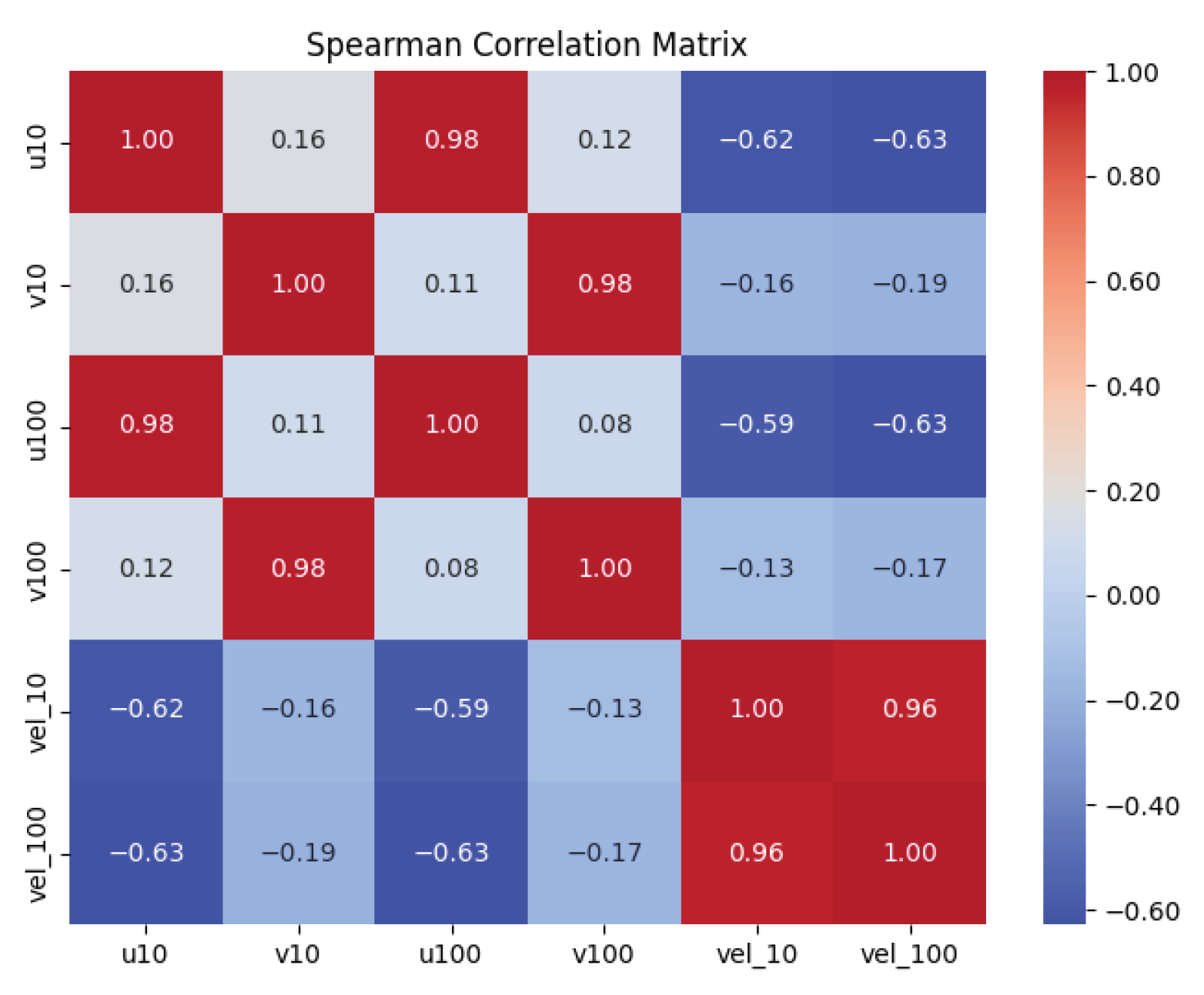
The Spearman correlation matrix is shown in Figure A2. The 10 m and 100 m wind components exhibit strong vertical coherence, with correlations of 0.98 for both zonal and meridional components and 0.96 for wind-speed magnitude. These results support the joint use of 10 m and 100 m wind fields as model inputs and provide empirical motivation for the vertical-profile consistency term used in the PC-SRCNN loss function.
The Spearman correlation matrix presented in Figure A2 reveals strong vertical coherence between wind components across altitudes. The zonal components and exhibit a very high correlation of 0.98, and the meridional components and show a correlation of 0.98, both indicating consistent vertical structure in the directional components. Wind speeds and display a correlation of 0.96, confirming strong consistency across heights. These inter-altitude correlations justify the joint use of 10 m and 100 m fields as complementary inputs to the model, as each variable retains coherent vertical structure while contributing independent information to the spatial reconstruction.
Figure A1.
Histograms of ERA5 reanalysis wind-field variables over Brazilian territory in January 2024: (a) zonal component ; (b) zonal component ; (c) meridional component ; (d) meridional component ; (e) wind-speed magnitude ; and (f) wind-speed magnitude . All variables are expressed in m/s, and subscripts indicate height above ground level in metres. Data from [1].
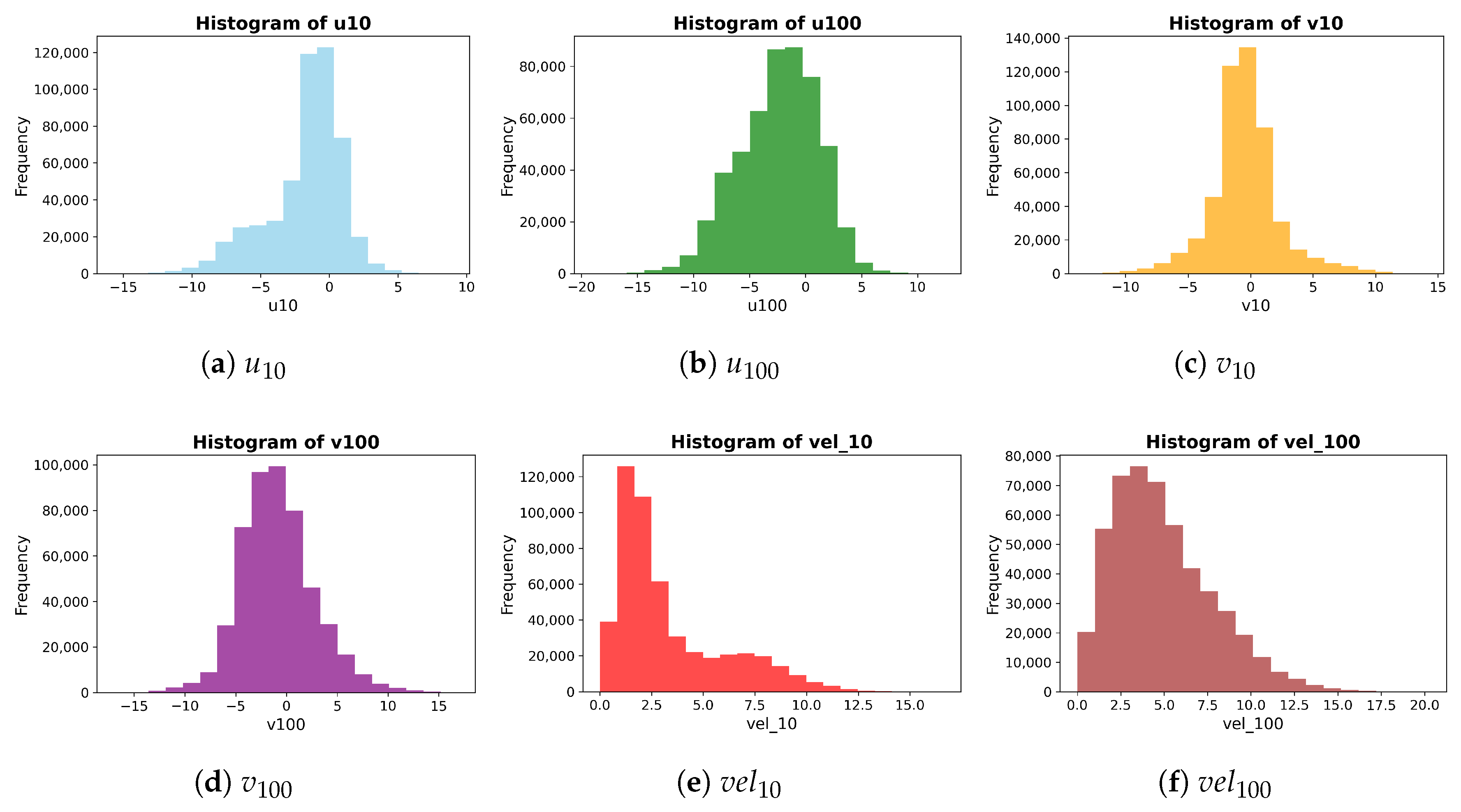
Table A1.
Descriptive statistics and statistical test results for physical variables. Symbols: , mean; , minimum; , maximum; , standard deviation. All values are computed from the sample and represent sample estimates.
Figure A2.
Spearman correlation heatmap of ERA5 reanalysis wind field variables [1] over Brazilian territory (January 2024).
Appendix A.2. Hyperparameter Optimization Framework
This appendix note provides additional methodological details on the Bayesian optimization framework used for hyperparameter tuning. The loss formulations and validation metrics are described in the main text (Section 2.3) and are not repeated here.
Appendix A.2.1. Bayesian Optimization Formulation
Bayesian optimization was used to tune the architectural and loss-weighting hyperparameters of the neural-network models using the Keras Tuner framework [62]. Bayesian optimization is appropriate for this task because each candidate model configuration is computationally expensive to evaluate, and the objective function is noisy due to stochastic neural-network training and spatial cross-validation.
The optimization problem can be written as
where denotes a candidate hyperparameter vector, is the bounded search domain, and is the objective function. Since model training is based on loss minimization, the objective can be interpreted as maximizing the negative validation loss:
Noisy function evaluations are represented as
Appendix A.2.2. Gaussian-Process Surrogate Model
A Gaussian Process (GP) was used as the surrogate model in Bayesian optimization. A GP defines a probability distribution over functions and is fully specified by a mean function and covariance function :
Assuming a zero prior mean, , the covariance function determines the smoothness and correlation structure of the surrogate model. A squared-exponential kernel was used:
where C is the length-scale parameter controlling the smoothness of the surrogate function.
Given observed hyperparameter configurations and objective values , the kernel matrix is defined as
For a new candidate point , the joint Gaussian distribution of observed outputs and the unknown function value is
where
The posterior predictive mean and variance are
Appendix A.2.3. Acquisition Function
The acquisition function determines which hyperparameter configuration should be evaluated next by balancing exploration and exploitation. Expected Improvement (EI) was used as the acquisition criterion [65,66,67,68,69,70]. Let
denote the best observed configuration. The improvement obtained by evaluating a new candidate is
Taking the expectation of under the GP posterior gives
where
and and are the cumulative distribution function and probability density function of the standard normal distribution, respectively.
Appendix A.2.4. Hyperparameter Search Space
The search was conducted over a maximum of 50 trials, including 15 randomly sampled initial points used to initialize the Gaussian-process surrogate. Each candidate configuration was trained for up to 50 epochs using a batch size of 8. Early stopping was applied with a patience of 17 epochs, monitored on the training loss. The learning rate was reduced by a factor of 0.95 whenever no improvement was observed for 15 consecutive epochs.
The hyperparameter search space is summarized in Table A2.
Table A2.
Hyperparameter search space used during Bayesian optimization.
Appendix A.2.5. Computational Environment
All computational experiments were conducted on a standard workstation equipped with an Intel Core i5-11400F processor, 32 GB of RAM, and an NVIDIA RTX 4060 GPU. This setup demonstrates that the proposed framework can be implemented without specialized high-performance computing infrastructure.
References
- Hersbach, H.; Bell, B.; Berrisford, P.; Biavati, G.; Horányi, A.; Muñoz Sabater, J.; Nicolas, J.; Peubey, C.; Radu, R.; Rozum, I.; et al. ERA5 Hourly Data on Single Levels from 1940 to Present. Copernicus Climate Change Service (C3S) Climate Data Store (CDS). 2023. Available online: https://cds.climate.copernicus.eu/datasets/reanalysis-era5-single-levels?tab=overview (accessed on 8 November 2025).
- Ding, J.-W.; Hsieh, I.-Y.L. Super-Resolution Wind Mapping with Deep Learning for Scalable Renewable Energy Planning. Commun. Earth Environ. 2026, 7, 51. [Google Scholar] [CrossRef] [Scilit]
- Lin, C.; Tie, R.; Yi, S.; Liu, D.; Zhong, X.; Hu, Z.; Li, H. Reconstructing Fine-Scale 3D Wind Fields with Terrain-Informed Machine Learning. Nat. Commun. 2026, 17, 3713. [Google Scholar] [CrossRef] [Scilit] [PubMed]
- Krusche, N.; Peralta, C.; Chang, C.-Y.; Stoevesandt, B. Wind Power Energy in Southern Brazil: Evaluation Using a Mesoscale Meteorological Model. Energy Procedia 2015, 76, 164–168. [Google Scholar] [CrossRef] [Scilit]
- Rosende, C.; Sauma, E.; Harrison, G.P. Effect of Climate Change on Wind Speed and Its Impact on Optimal Power System Expansion Planning: The Case of Chile. Energy Econ. 2019, 80, 434–451. [Google Scholar] [CrossRef] [Scilit]
- Paola, F.; Cimini, D.; De Natale, M.P.; Gallucci, D.; Gentile, S.; Geraldi, E.; Larosa, S.; Nilo, S.; Ricciardelli, E.; Ripepi, E.; et al. Wind Speed Downscaling of the WRF Model at Subkilometer Scale in Complex Terrain for Wind Power Applications. IEEE J. Sel. Top. Appl. Earth Obs. Remote Sens. 2024, 17, 9139–9177. [Google Scholar] [CrossRef] [Scilit]
- Silva, T.; Costa, A.; Vilela, O.C.; Willmersdorf, R.; dos Santos Júnior, J.V.; Alves, L.H.B.; Tyaquiçã, P.; de Lima, M.F.S.; de Souza, H.R.B.; Veleda, D. Application of the WRF Model for Operational Wind Power Forecasting in Northeast Brazil. Energies 2025, 18, 5731. [Google Scholar] [CrossRef] [Scilit]
- Li, L. Geographically Weighted Machine Learning and Downscaling for High-Resolution Spatiotemporal Estimations of Wind Speed. Remote Sens. 2019, 11, 1378. [Google Scholar] [CrossRef] [Scilit]
- Pryor, S.C.; Barthelmie, R.J.; Bukovsky, M.S.; Leung, L.R.; Sakaguchi, K. Climate Change Impacts on Wind Power Generation. Nat. Rev. Earth Environ. 2020, 1, 627–643. [Google Scholar] [CrossRef] [Scilit]
- Hu, J.; Mu, J.; Huang, X.; Wu, X. Unsupervised Meteorological Downscaling Based on Dual Learning and Subgrid-Scale Auxiliary Information. Adv. Atmos. Sci. 2025, 42, 53–66. [Google Scholar] [CrossRef] [Scilit]
- Kashinath, K.; Mustafa, M.; Albert, A.; Wu, J.-L.; Jiang, C.; Esmaeilzadeh, S.; Azizzadenesheli, K.; Wang, R.; Chattopadhyay, A.; Singh, A.; et al. Physics-informed machine learning: Case studies for weather and climate modelling. Philos. Trans. R. Soc. A 2021, 379, 20200093. [Google Scholar] [CrossRef] [Scilit] [PubMed]
- Balog, I.; Caputo, G.; Iatauro, D.; Signoretti, P.; Spinelli, F. Downscaling of Hourly Climate Data for the Assessment of Building Energy Performance. Sustainability 2023, 15, 2762. [Google Scholar] [CrossRef] [Scilit]
- Buster, G.; Rossol, M.; Maclaurin, G.; Xie, Y.; Sengupta, M. A Physical Downscaling Algorithm for the Generation of High-Resolution Spatiotemporal Solar Irradiance Data. Sol. Energy 2021, 216, 508–517. [Google Scholar] [CrossRef] [Scilit]
- Omoyele, O.; Hoffmann, M.; Weinand, J.M.; Larraneta, M.; Linßen, J.; Stolten, D. A High-Resolution Downscaling Approach for Solar Irradiance Using Statistical Parameter Matching. Renew. Energy 2026, 256, 124551. [Google Scholar] [CrossRef] [Scilit]
- He, X.; Ye, B.; Gu, C. AI in Wind Energy Prediction and Optimization Techniques Review. In Proceedings of the 2025 IEEE International Symposium on the Application of Artificial Intelligence in Electrical Engineering (AAIEE), Beijing, China, 25–28 April 2025; pp. 887–891. [Google Scholar] [CrossRef] [Scilit]
- Wadood, H.; Haris, M.; Hassan, A.; Malik, M.O.; Yousaf, H.; Ullah, K. Deep Learning Applications for Wind Energy Forecasting in Smart Grids. In Proceedings of the International Conference on Engineering and Emerging Technologies (ICEET), Dubai, United Arab Emirates, 27–28 December 2024. [Google Scholar] [CrossRef] [Scilit]
- Belletreche, M.; Bailek, N.; Abotaleb, M.; Bouchouicha, K.; Zerouali, B.; Guermoui, M.; Kuriqi, A.; Alharbi, A.H.; Khafaga, D.S.; EL-Shimy, M.; et al. Hybrid Attention-Based Deep Neural Networks for Short-Term Wind Power Forecasting Using Meteorological Data in Desert Regions. Sci. Rep. 2024, 14, 21842. [Google Scholar] [CrossRef] [Scilit] [PubMed]
- Birudaraju, H.; Sailaja, K.; Sreedevi, V.; Viswanathan, R.; Vandaarkuzhali, S. Integrating Machine Learning (ML) and Deep Learning (DL) Methods to Produce Reliable Wind Power Predictions. In Proceedings of the 2024 2nd International Conference on Computational and Characterization Techniques in Engineering and Sciences (IC3TES), Lucknow, India, 15–16 November 2024. [Google Scholar] [CrossRef] [Scilit]
- Pham, T.S.; Nguyen, D.H.; Phan, N.D.M. Wind Energy Forecasting: A Comparative Analysis of Machine Learning Approaches. In Proceedings of the 2023 8th International Scientific Conference on Applying New Technology in Green Buildings (ATiGB), Danang, Vietnam, 10–11 November 2023; pp. 195–200. [Google Scholar] [CrossRef] [Scilit]
- Daenens, S.; Vervlimmeren, I.; Verstraeten, T.; Daems, P.-J.; Nowé, A.; Helsen, J. Power Prediction Using High-Resolution SCADA Data with a Farm-Wide Deep Neural Network Approach. J. Phys. Conf. Ser. 2024, 2767, 092014. [Google Scholar] [CrossRef] [Scilit]
- Pandit, R.; Astolfi, D.; Hong, J.; Infield, D.; Santos, M. SCADA Data for Wind Turbine Data-Driven Condition/Performance Monitoring: A Review on State-of-Art, Challenges and Future Trends. Wind Eng. 2023, 47, 422–441. [Google Scholar] [CrossRef] [Scilit]
- Mohd, Y.; Singh, H. Machine Learning for Analysis and Prediction of Wind Energy. In Proceedings of the International Conference on Circuit Power and Computing Technologies (ICCPCT), Kollam, India, 10–11 August 2023; pp. 1438–1445. [Google Scholar] [CrossRef] [Scilit]
- Liu, Z.; Guo, H.; Zhang, Y.; Zuo, Z. A Comprehensive Review of Wind Power Prediction Based on Machine Learning: Models, Applications, and Challenges. Energies 2025, 18, 350. [Google Scholar] [CrossRef] [Scilit]
- Cao, J.; Farnham, D.J.; Lall, U. Spatial–Temporal Wind Field Projection by Artificial Neural Networks. arXiv 2017, arXiv:1712.05293. [Google Scholar] [CrossRef] [Scilit]
- Acker, T.L.; Williams, S.K.; Duque, E.P.N.; Brummels, G.; Buechler, J. Wind Resource Assessment in the State of Arizona: Inventory, Capacity Factor, and Cost. Renew. Energy 2007, 32, 1453–1466. [Google Scholar] [CrossRef] [Scilit]
- Zalhaf, A.S.; Elboshy, B.; Kotb, K.M.; Han, Y.; Almaliki, A.H.; Aly, R.M.H.; Elkadeem, M.R. A High-Resolution Wind Farms Suitability Mapping Using GIS and Fuzzy AHP Approach: A National-Level Case Study in Sudan. Sustainability 2022, 14, 358. [Google Scholar] [CrossRef] [Scilit]
- Turkovska, O.; Castro, G.; Klingler, M.; Nitsch, F.; Regner, P.; Soterroni, A.C.; Schmidt, J. Land-Use Impacts of Brazilian Wind Power Expansion. Environ. Res. Lett. 2021, 16, 024010. [Google Scholar] [CrossRef] [Scilit]
- Davis, N.N.; Badger, J.; Hahmann, A.N.; Hansen, B.O.; Mortensen, N.G.; Kelly, M.; Larsén, X.G.; Olsen, B.T.; Floors, R.; Lizcano, G.; et al. The Global Wind Atlas: A High-Resolution Dataset of Climatologies and Associated Web-Based Application. Bull. Am. Meteorol. Soc. 2023, 104, E1507–E1525. [Google Scholar] [CrossRef] [Scilit]
- Rehman, S.; Zayed, M.E.; Syed, A.H.; Ghazy, M.; Irshad, K.; Al-Shaikhi, A.; Mohandes, M.A.; Alhems, L.M. Assessment of Offshore Wind Power Potential in Saudi Arabia’s Red Sea: Insights into Fixed-Bottom and Floating Offshore Technologies. Results Eng. 2026, 29, 108626. [Google Scholar] [CrossRef] [Scilit]
- Vinhoza, A.; Schaeffer, R. Brazil’s Offshore Wind Energy Potential Assessment Based on a Spatial Multi-Criteria Decision Analysis. Renew. Sustain. Energy Rev. 2021, 146, 111185. [Google Scholar] [CrossRef] [Scilit]
- de Carvalho, O.L.F.; de Carvalho Junior, O.A.; de Albuquerque, A.O.; Orlandi, A.G.; Hirata, I.; Borges, D.L.; Gomes, R.A.T.; Guimarães, R.F. A Data-Centric Approach for Wind Plant Instance-Level Segmentation Using Semantic Segmentation and GIS. Remote Sens. 2023, 15, 1240. [Google Scholar] [CrossRef] [Scilit]
- Alkhalidi, M.; Al-Dabbous, A.; Al-Dabbous, S.; Alzaid, D. Evaluating the Accuracy of the ERA5 Model in Predicting Wind Speeds Across Coastal and Offshore Regions. J. Mar. Sci. Eng. 2025, 13, 149. [Google Scholar] [CrossRef] [Scilit]
- Gasset, N.; Landry, M.; Gagnon, Y. A Comparison of Wind Flow Models for Wind Resource Assessment in Wind Energy Applications. Energies 2012, 5, 4288–4322. [Google Scholar] [CrossRef] [Scilit]
- Reichstein, M.; Camps-Valls, G.; Stevens, B.; Jung, M.; Denzler, J.; Carvalhais, N.; Prabhat. Deep learning and process understanding for data-driven Earth system science. Nature 2019, 566, 195–204. [Google Scholar] [CrossRef] [Scilit] [PubMed]
- Vandal, T.; Kodra, E.; Ganguly, S.; Michaelis, A.; Nemani, R.; Ganguly, A.R. DeepSD: Generating High Resolution Climate Change Projections through Single Image Super-Resolution. In Proceedings of the 23rd ACM SIGKDD International Conference on Knowledge Discovery and Data Mining (KDD ’17), Halifax, NS, Canada, 13–17 August 2017; pp. 1663–1672. [Google Scholar] [CrossRef] [Scilit]
- Baki, H.; Basu, S. Estimating High-Resolution Profiles of Wind Speeds from a Global Reanalysis Dataset Using TabNet. Environ. Data Sci. 2025, 3, e32. [Google Scholar] [CrossRef] [Scilit]
- Rezvov, V.; Krinitskiy, M.; Gulev, S. Approximation of High-Resolution Surface Wind Speed in the North Atlantic Using Discriminative and Generative Neural Models Based on RAS-NAAD 40-Year Hindcast. In Proceedings of the 6th International Workshop on Deep Learning in Computational Physics (DLCP2022), Dubna, Russia, 6–8 July 2022; Volume 429. [Google Scholar]
- Adytia, D.; Latifah, A.L.; Saepudin, D.; Tarwidi, D.; Pudjaprasetya, S.R.; Husrin, S.; Sopaheluwakan, A.; Prasetya, G. A Deep Learning Approach for Wind Downscaling Using Spatially Correlated Global Wind Data. Int. J. Data Sci. Anal. 2025, 20, 2721–2735. [Google Scholar] [CrossRef] [Scilit]
- Helgason, G.B. Downscaling Wind Fields Using Deep Learning. Master’s Thesis, Technical University of Denmark (DTU), Roskilde, Denmark, 2022. Available online: https://backend.orbit.dtu.dk/ws/portalfiles/portal/337856561/Thesis_GBH_DTU_Final.pdf (accessed on 4 August 2026).
- Lian, J.; Huang, S.; Shao, J.; Chen, P.; Tang, S.; Lu, Y.; Yu, H. TerraWind: A deep learning-based near-surface winds downscaling model for complex terrain region. Geophys. Res. Lett. 2024, 51, e2024GL112124. [Google Scholar] [CrossRef] [Scilit]
- Kolukula, S.S.; Murty, P.L.N.; Baduru, B.; Sharath, D.; Francis, P.A. Downscaling of Wind Fields on the East Coast of India Using Deep Convolutional Neural Networks and Their Applications in Storm Surge Computations. J. Water Clim. Chang. 2024, 15, 1612–1628. [Google Scholar] [CrossRef] [Scilit]
- He, Z.; Liu, L.; Huang, J.; Dong, X.; Zhao, H.; Li, B. Location-Aware Memory Enhancement for Wind Speed Super-Resolution. In Proceedings of the 2025 6th International Conference on Computer Vision, Image and Deep Learning (CVIDL), Ningbo, China, 23–25 May 2025; pp. 730–735. [Google Scholar] [CrossRef] [Scilit]
- INMET. Dados de Estacões Automáticas Meteorológicas—Janeiro 2024; Instituto Nacional de Meteorologia: Brasilia, Brazil, 2024. Available online: https://bdmep.inmet.gov.br/ (accessed on 26 January 2024).
- The Wind Atlas. Global Wind Atlas. 2024. Available online: https://globalwindatlas.info (accessed on 26 January 2024).
- Monin, A.S.; Obukhov, A.M. Basic Laws of Turbulent Mixing in the Surface Layer of the Atmosphere. Contrib. Geophys. Inst. Acad. Sci. USSR 1954, 151, e187. [Google Scholar]
- Stull, R.B. An Introduction to Boundary Layer Meteorology; Springer Science & Business Media: Dordrecht, The Netherlands, 2012; Volume 13. [Google Scholar]
- Arya, P.S. Introduction to Micrometeorology; Elsevier: Amsterdam, The Netherlands, 2001; Volume 79. [Google Scholar]
- Troen, I.; Petersen, E.L. European Wind Atlas; Risø National Laboratory: Roskilde, Denmark, 1989. [Google Scholar]
- Dong, C.; Loy, C.C.; He, K.; Tang, X. Image Super-Resolution Using Deep Convolutional Networks. IEEE Trans. Pattern Anal. Mach. Intell. 2015, 38, 295–307. [Google Scholar] [CrossRef] [Scilit] [PubMed]
- Kim, J.; Lee, J.K.; Lee, K.M. Accurate Image Super-Resolution Using Very Deep Convolutional Networks. In Proceedings of the IEEE Conference on Computer Vision and Pattern Recognition (CVPR), Las Vegas, NV, USA, 27–30 June 2016; pp. 1646–1654. [Google Scholar] [CrossRef] [Scilit]
- Lim, B.; Son, S.; Kim, H.; Nah, S.; Mu Lee, K. Enhanced Deep Residual Networks for Single Image Super-Resolution. In Proceedings of the IEEE Conference on Computer Vision and Pattern Recognition Workshops, Honolulu, HI, USA, 21–26 July 2017; pp. 136–144. [Google Scholar]
- Tai, Y.; Yang, J.; Liu, X. Image Super-Resolution via Deep Recursive Residual Network. In Proceedings of the IEEE Conference on Computer Vision and Pattern Recognition, Honolulu, HI, USA, 21–26 July 2017; pp. 3147–3155. [Google Scholar]
- Ledig, C.; Theis, L.; Huszár, F.; Caballero, J.; Cunningham, A.; Acosta, A.; Aitken, A.; Tejani, A.; Totz, J.; Wang, Z.; et al. Photo-Realistic Single Image Super-Resolution Using a Generative Adversarial Network. In Proceedings of the IEEE Conference on Computer Vision and Pattern Recognition, Honolulu, HI, USA, 21–26 July 2017; pp. 4681–4690. [Google Scholar]
- Zhang, Y.; Tian, Y.; Kong, Y.; Zhong, B.; Fu, Y. Residual Dense Network for Image Super-Resolution. In Proceedings of the IEEE Conference on Computer Vision and Pattern Recognition, Athens, Greece, 7–10 October 2018; pp. 2472–2481. [Google Scholar]
- Yasuda, Y.; Onishi, R.; Matsuda, K. Super-Resolution of Three-Dimensional Temperature and Velocity for Building-Resolving Urban Micrometeorology Using Physics-Guided Convolutional Neural Networks with Image Inpainting Techniques. Build. Environ. 2023, 213, 110613. [Google Scholar] [CrossRef] [Scilit]
- Lockwood, J.W.; Gori, A.; Gentine, P. A Generative Super-Resolution Model for Enhancing Tropical Cyclone Wind Field Intensity and Resolution. J. Geophys. Res. Mach. Learn. Comput. 2024, 1, e2024JH000375. [Google Scholar] [CrossRef] [Scilit]
- LeCun, Y.; Bottou, L.; Bengio, Y.; Haffner, P. Gradient-Based Learning Applied to Document Recognition. Proc. IEEE 2002, 86, 2278–2324. [Google Scholar]
- Goodfellow, I.; Bengio, Y.; Courville, A. Deep Learning; MIT Press: Cambridge, MA, USA, 2016. [Google Scholar]
- Raissi, M.; Perdikaris, P.; Karniadakis, G.E. Physics-Informed Neural Networks: A Deep Learning Framework for Solving Forward and Inverse Problems Involving Nonlinear Partial Differential Equations. J. Comput. Phys. 2019, 378, 686–707. [Google Scholar] [CrossRef] [Scilit]
- Geneva, N.; Zabaras, N. Modeling the Dynamics of PDE Systems with Physics-Constrained Deep Auto-Regressive Networks. J. Comput. Phys. 2020, 403, 109056. [Google Scholar] [CrossRef] [Scilit]
- Mao, Z.; Jagtap, A.D.; Karniadakis, G.E. Physics-Informed Neural Networks for High-Speed Flows. Comput. Methods Appl. Mech. Eng. 2020, 360, 112789. [Google Scholar] [CrossRef] [Scilit]
- O’Malley, T.; Bursztein, E.; Long, J.; Chollet, F.; Jin, H.; Invernizzi, L.; others. Keras Tuner. 2019. Available online: https://github.com/keras-team/keras-tuner (accessed on 26 January 2024).
- Diebold, F.X.; Mariano, R.S. Comparing Predictive Accuracy. J. Bus. Econ. Stat. 1995, 13, 253–263. [Google Scholar] [CrossRef] [Scilit]
- Coroneo, L.; Iacone, F. Testing for Equal Predictive Accuracy with Strong Dependence. Int. J. Forecast. 2025, 41, 1073–1092. [Google Scholar] [CrossRef] [Scilit]
- Mockus, J.; Tiesis, V.; Zilinskas, A. The Application of Bayesian Methods for Seeking the Extremum. In Toward Global Optimization; Dixon, L., Szego, G., Eds.; North-Holland Publishing Company: Amsterdam, The Netherlands, 1978; Volume 2. [Google Scholar]
- Shahriari, B.; Swersky, K.; Wang, Z.; Adams, R.P.; De Freitas, N. Taking the Human Out of the Loop: A Review of Bayesian Optimization. Proc. IEEE 2015, 104, 148–175. [Google Scholar] [CrossRef] [Scilit]
- Snoek, J.; Rippel, O.; Swersky, K.; Kiros, R.; Satish, N.; Sundaram, N.; Patwary, M.; Prabhat, M.; Adams, R. Scalable Bayesian Optimization Using Deep Neural Networks. In International Conference on Machine Learning; PMLR: Cambridge, MA, USA, 2015; pp. 2171–2180. [Google Scholar]
- Ryan, E.G.; Drovandi, C.C.; McGree, J.M.; Pettitt, A.N. A Review of Modern Computational Algorithms for Bayesian Optimal Design. Int. Stat. Rev. 2016, 84, 128–154. [Google Scholar] [CrossRef] [Scilit]
- Williams, C.K.I.; Rasmussen, C.E. Gaussian Processes for Machine Learning; MIT Press: Cambridge, MA, USA, 2006; Volume 2. [Google Scholar]
- Bartók, A.P.; Csányi, G. Gaussian Approximation Potentials: A Brief Tutorial Introduction. Int. J. Quantum Chem. 2015, 115, 1051–1057. [Google Scholar] [CrossRef] [Scilit]
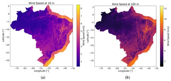
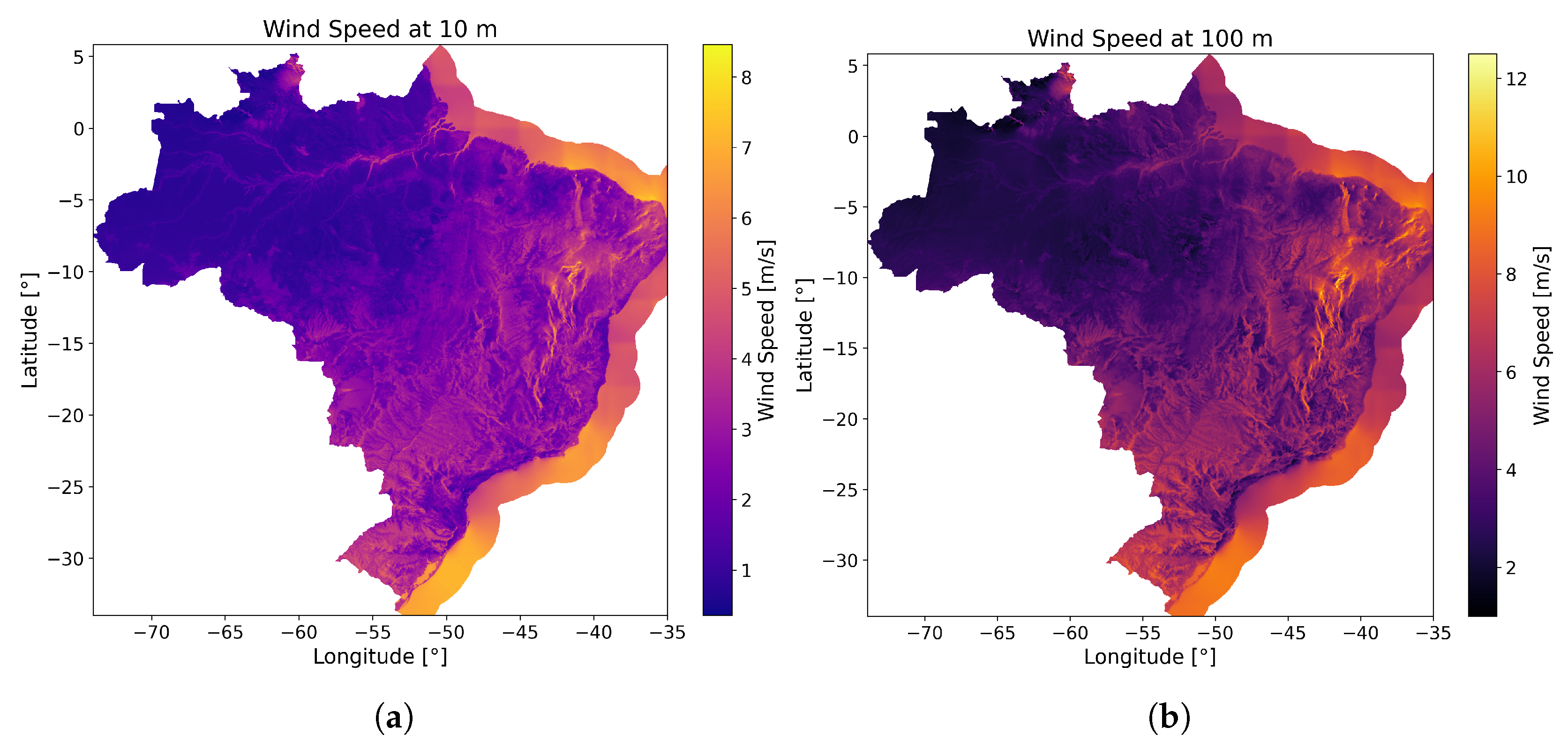
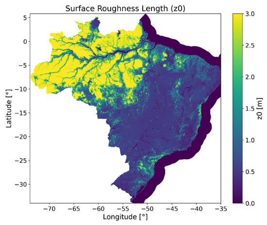
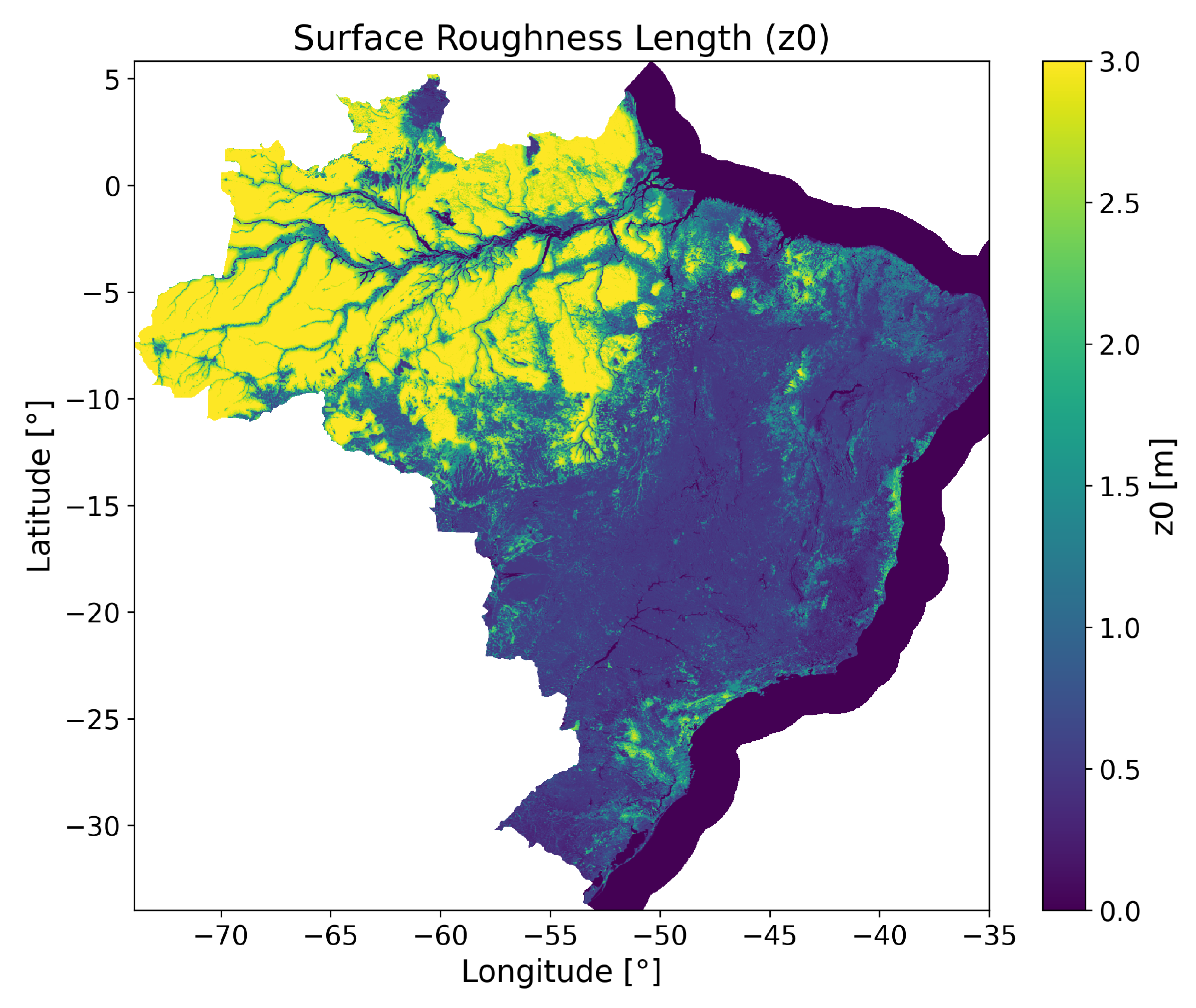
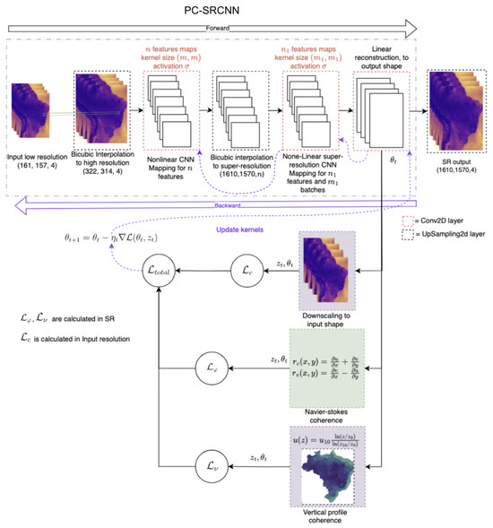
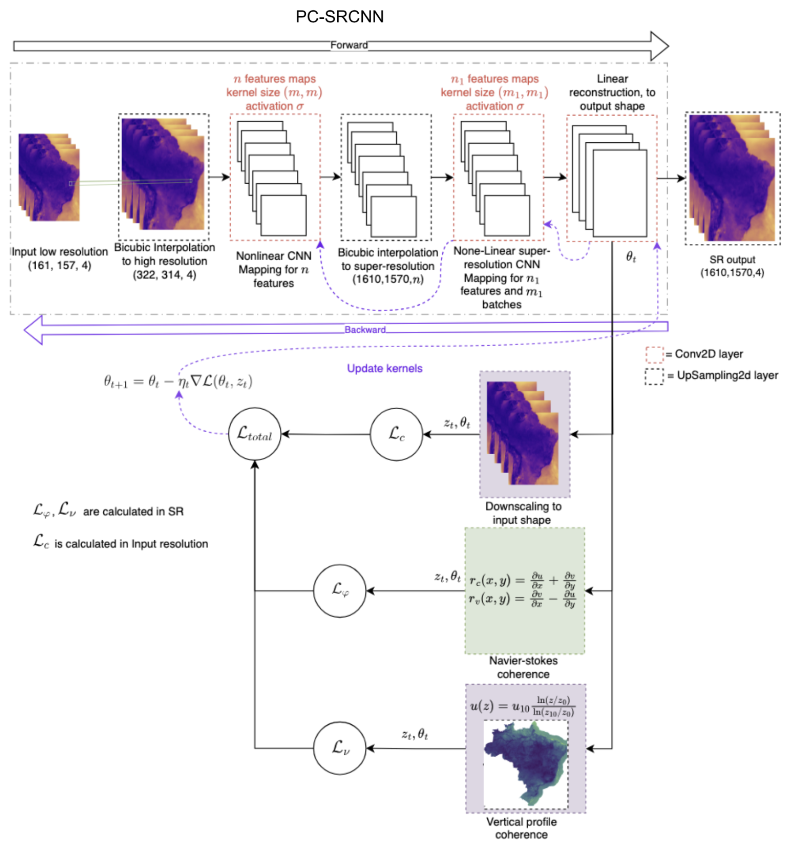
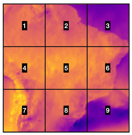
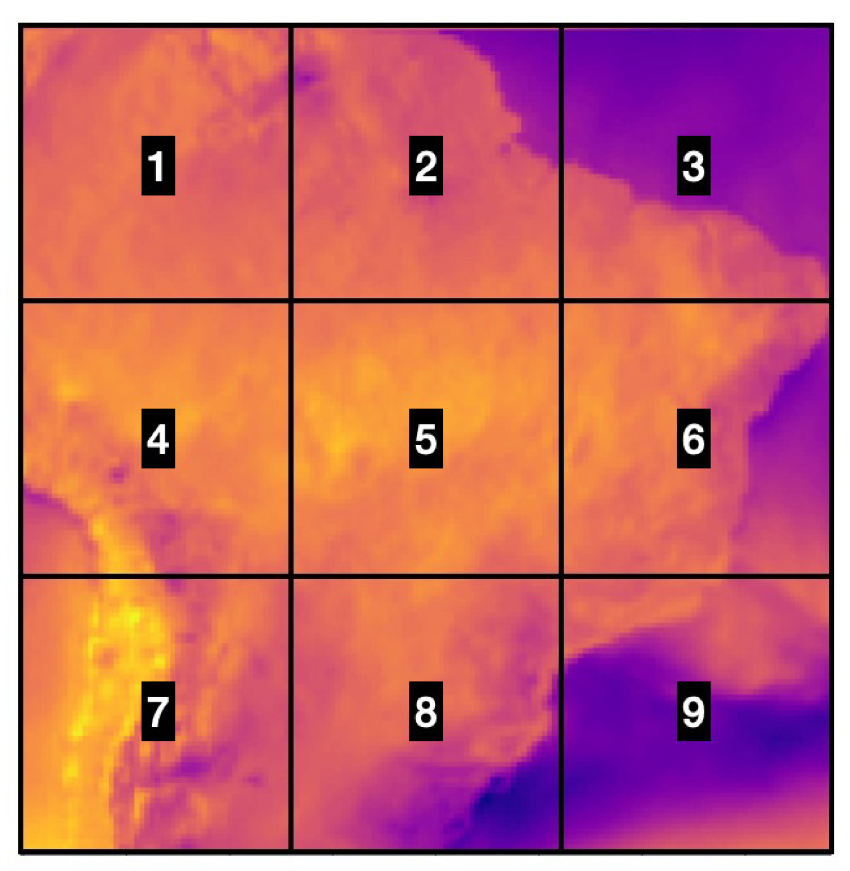
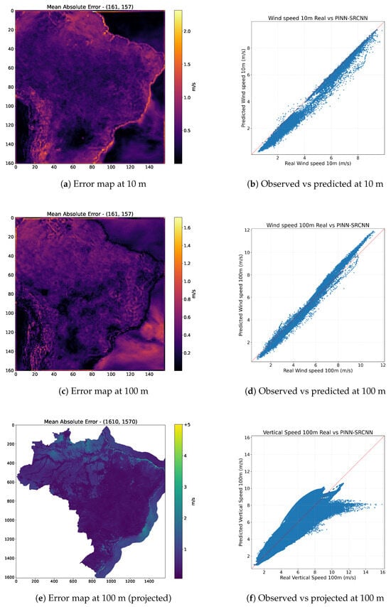
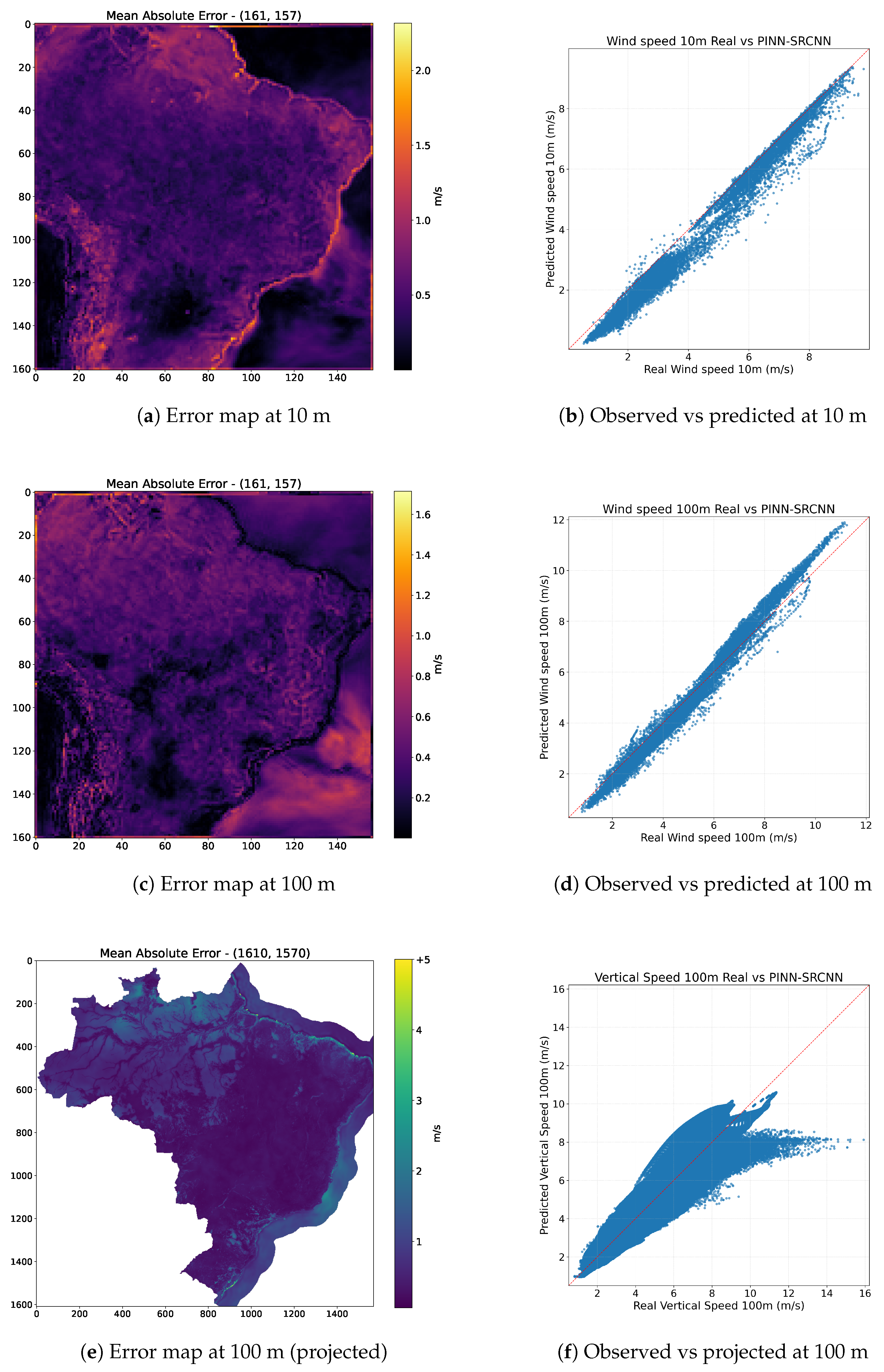

Disclaimer/Publisher’s Note: The statements, opinions and data contained in all publications are solely those of the individual author(s) and contributor(s) and not of MDPI and/or the editor(s). MDPI and/or the editor(s) disclaim responsibility for any injury to people or property resulting from any ideas, methods, instructions or products referred to in the content. |
© 2026 by the authors. Licensee MDPI, Basel, Switzerland. This article is an open access article distributed under the terms and conditions of the Creative Commons Attribution (CC BY) license.