


Abstract
Reliable state of health (SOH) estimation provides important support for safety management and efficient operation of lithium-ion battery energy storage systems. To address the limitations of existing SOH estimation methods in terms of feature interpretability, joint modeling of local variations and overall morphological characteristics within each feature segment, and the rationality of model hyperparameter configuration, this study proposes a hybrid data-driven SOH estimation method integrating interpretable feature construction, an improved Transformer, and Bayesian optimization (BO). Specifically, raw charging data are first converted into incremental capacity (IC) curves based on incremental capacity analysis, and IC peaks are dynamically located in different cycles. Local voltage–capacity segments around the IC peak voltage are then extracted as interpretable input features closely related to battery aging. Subsequently, the Transformer encoder is improved by incorporating patch embedding and a multi-head differential self-attention mechanism, thereby enhancing the model’s ability to jointly capture local variations and overall morphological characteristics within each cycle-wise feature segment. BO is further employed to adaptively optimize key model hyperparameters. Experimental results on the CALCE-CS2 and CALCE-CX2 battery datasets show that the proposed BO-PatchDiffFormer model can provide accurate and stable SOH estimation in both comparative and generalization experimental scenarios. Compared with the best-performing baseline model, the maximum reductions in RMSE and MAE on the four CS2 test batteries reach 31.81% and 23.76%, respectively. In the generalization experiments, the average RMSE and MAE on the two CX2 test batteries are 1.6039% and 1.3081%, respectively. In addition, the maximum model size is only 2.07 MB, and the single-sample inference time remains within 0.84–1.18 ms, indicating good potential for practical deployment and application.
1. Introduction
Driven by the development of new power systems and the grid-scale integration of renewable energy, battery energy storage systems (BESSs) contribute significantly to power-system frequency regulation and the secure, stable operation of power grids [1,2]. Lithium-ion batteries (LIBs) are extensively adopted in BESSs, mainly benefiting from their high energy density and long cycle life [3]. However, prolonged charge–discharge operation causes gradual degradation of LIBs. Such degradation may increase the likelihood of electrolyte leakage and local short-circuit faults, and in severe cases can trigger safety accidents, including fire or explosion [4,5]. Accordingly, accurate estimation of the state of health (SOH) of LIBs is essential for enhancing the operational safety, reliability, and economic efficiency of BESSs [6].
SOH serves as a key metric for characterizing the aging degree of LIBs. Existing SOH estimation methods for LIBs are generally classified into experimental measurement methods, model-driven methods, and data-driven methods [7,8,9]. Experimental measurement methods generally obtain battery capacity by carrying out full charge–discharge tests and calculating the accumulated charge through ampere-hour integration, which enables relatively reliable SOH estimation [10]. Although such methods have low computational complexity, they are time-consuming and costly in experiments, which limits their applicability in online monitoring and real-time SOH estimation scenarios [11]. Model-driven methods estimate SOH by describing battery electrochemical behavior or circuit characteristics through electrochemical models and equivalent circuit models [12,13]. Nevertheless, their performance depends strongly on accurate parameter identification and prior knowledge of battery aging mechanisms, and the estimation accuracy is also affected by degradation-related failure mechanisms. These factors limit the practical use of model-driven methods [14].
Recent advances in artificial intelligence have promoted the development of data-driven approaches for LIB SOH estimation, particularly those based on machine learning and deep learning. These approaches learn the mapping relationship between degradation-related features and SOH from historical cycling data, without requiring detailed modeling of the internal electrochemical processes of batteries [15,16,17]. Chen et al. proposed an SOH estimation method for LIBs based on the extreme gradient boosting (XGBoost) model. This method extracts statistical and geometric features from the constant-voltage charging process and combines them with the average constant-voltage charging current to construct combined feature inputs, thereby achieving good SOH estimation performance [18]. Zhang et al. proposed an SOH estimation method for LIBs based on the long short-term memory (LSTM) network. By constructing multidimensional health features and adopting a segmented LSTM modeling strategy, this method alleviates the error accumulation effect in long-sequence prediction and improves SOH estimation accuracy [19].
Although data-driven methods have achieved good performance in SOH estimation tasks for LIBs, existing studies still have some limitations. First, although deep learning models have strong nonlinear feature extraction capabilities, their network structures have inherent “black-box” characteristics. As a result, the correspondence between the extracted features and the internal aging mechanisms of batteries is not sufficiently clear, leading to insufficient physical interpretability in the feature extraction process of the models [20,21]. Second, under the combined influence of capacity regeneration and random fluctuations, the SOH sequence of LIBs exhibits multiple local recoveries and short-term nonmonotonic fluctuations during cyclic aging. This makes it difficult for models to distinguish transient capacity recovery from the underlying degradation state, further increasing the difficulty of accurate SOH estimation [22,23]. In addition, the prediction performance of deep learning models largely depends on hyperparameter settings [24]. Conventional manual hyperparameter tuning is often inefficient and may become trapped in local optima, making it difficult to obtain consistently favorable SOH estimation performance across different batteries [25,26].
Existing studies have begun to make corresponding improvements to address the above issues. Luan et al. introduced incremental capacity analysis (ICA) into the SOH estimation task for LIBs. By differentiating the capacity–voltage relationship during the charging stage, the aging information that is difficult to directly identify from the raw charging curves is transformed into IC curve features with distinct peaks, thereby strengthening the correlation between the feature extraction process and the internal electrochemical degradation mechanisms of batteries [27]. Xu et al. developed an LSTM-based SOH estimation method by incorporating data features and a spatiotemporal attention mechanism to handle trend nonlinearity and capacity regeneration in LIB degradation sequences. In their method, the original input information is separated into trend-related and non-trend-related components, and spatiotemporal features are extracted from multidimensional non-trend features through the spatiotemporal attention mechanism. Then, model inputs containing trend features, spatiotemporal features, and capacity sequences are constructed, and SOH estimation is finally performed using the LSTM network [28]. Wang et al. developed a WOA-BiLSTM model by introducing the whale optimization algorithm (WOA) into the BiLSTM network. In this method, degradation-related inputs are constructed from IC curves and differential voltage curves, while WOA is adopted to determine suitable hyperparameters for the BiLSTM model. This strategy improves both SOH estimation accuracy and generalization performance [29].
Although significant progress has been made in current studies, most existing methods focus on improving a single issue, making it difficult to simultaneously consider interpretable feature construction, the joint modeling of local variations and overall morphological characteristics within each cycle-wise feature segment, and the adaptive optimization of model hyperparameters within a unified framework. Therefore, IC-peak-centered local voltage–capacity segments are constructed in this study as interpretable inputs that reflect the battery degradation process. On this basis, the BO-PatchDiffFormer model combines patch embedding with a multi-head differential self-attention mechanism to jointly model local variations and overall morphological characteristics within each cycle-wise feature segment. Bayesian optimization is further introduced to adaptively optimize key model hyperparameters, thereby achieving accurate SOH estimation for LIBs.
The main contributions of this study can be summarized as follows:
(1) A local voltage–capacity segment construction method centered on IC peaks is proposed. This method determines the peak positions of IC curves in different cycles through ICA and constructs local voltage windows centered on the corresponding peak positions. On this basis, voltage–capacity segments within the peak neighborhood are extracted, so that the input features correspond to the key electrochemical mechanisms of battery aging, thereby improving the physical interpretability of the feature construction process.
(2) A BO-PatchDiffFormer model is developed for SOH estimation. The constructed feature segments are first transformed into embedded representations using patch embedding and positional encoding. The standard self-attention in the Transformer encoder is then replaced with differential self-attention to emphasize degradation-sensitive patches and suppress redundant attention. This design enhances the joint modeling of local variations and overall morphological characteristics within each cycle-wise feature segment. Bayesian optimization is further employed to adaptively determine key hyperparameters, improving tuning efficiency and model stability.
(3) Experimental results on public aging datasets with two types of batteries confirm the advantages of the proposed method in estimation accuracy, generalization capability, and model stability. In addition, the results of model complexity and inference efficiency analyses show that the proposed method has low computational overhead and fast online inference speed, indicating good potential for deployment and practical application.
2. Materials
2.1. SOH Definition and Mathematical Expression
SOH quantifies the remaining electrical energy storage capability of a lithium-ion battery relative to its fresh state and is commonly expressed as a percentage [30]. In this study, based on the degree of battery capacity degradation, SOH is defined as the ratio of the current actual capacity of the battery to its initial capacity, as shown in Equation (1):
where represents the actual battery capacity at cycle , and is the initial capacity of the battery.
2.2. CALCE Battery Dataset
The experimental data were obtained from the CALCE-CS2 and CALCE-CX2 lithium-ion battery aging datasets provided by the Center for Advanced Life Cycle Engineering (CALCE), University of Maryland [31]. Both types of LIBs are prismatic, with LiCoO2 containing a small amount of Mn as the cathode material and graphite as the anode material. To examine whether the developed SOH estimation method remains robust across different batteries, CS2_35, CS2_36, CS2_37, and CS2_38 from the CS2 series are used for the main experiments, while CX2_34 and CX2_36 from the CX2 series are used for the generalization experiments.
The cyclic charge–discharge tests mainly consisted of two stages: a constant current–constant voltage (CC–CV) charging stage and a constant current (CC) discharging stage. The sampling frequency was 1/30 Hz, and the test temperature was 25 °C. During the charging process, the two types of LIBs were charged in CC mode at a constant current rate of 0.5 C until the charge cut-off voltage of 4.2 V was reached, and were then charged in CV mode until the current decreased to 0.05 A. During the discharging process, the two types of LIBs were discharged in CC mode at different constant current rates until the discharge cut-off voltage of 2.7 V was reached. The discharge current of CS2_35, CS2_36, CS2_37, and CS2_38 was 1.1 A, and their total numbers of cycles were 936, 976, 1043, and 1082, respectively. The discharge current of CX2_34 and CX2_36 was 1.35 A, and their total numbers of cycles were 1724 and 1958, respectively.
2.3. Data Preprocessing
Before feature extraction and model training, the raw charge–discharge data were preprocessed to improve data reliability. The raw charge–discharge data in the CALCE dataset contain a small number of invalid sampling points, such as missing values and infinite values, during data acquisition and storage. In this study, the raw charge–discharge data were first cleaned by removing invalid sampling points, and the data within each cycle were reordered according to the sampling time to ensure the consistency of discharge capacity calculation using the ampere-hour integration method. For cycle samples with incomplete data segments or those for which the discharge capacity could not be effectively calculated, they were regarded as invalid cycles and removed. After data cleaning, the numbers of valid cycles for CS2_35, CS2_36, CS2_37, and CS2_38 were 929, 922, 984, and 1069, respectively; and the numbers of valid cycles for CX2_34 and CX2_36 were 1721 and 1955, respectively.
During battery charge–discharge tests, the raw charge–discharge data, such as voltage and current, inevitably contain a certain amount of noise due to factors such as sensor accuracy and fluctuations in the test environment. Gaussian filtering was applied to smooth the raw charge–discharge data and suppress noise. The basic idea of Gaussian filtering is to assign different weights to the sampling data within the neighborhood of the target point according to the Gaussian function, and to obtain the smoothed data value through weighted averaging [32]. The Gaussian weighting function can be written as Equation (2):
where represents the relative position of a sampling point within the Gaussian kernel, represents the weight assigned by the Gaussian function to the corresponding sampling point, denotes the center of the Gaussian kernel and is set to zero, and denotes the standard deviation of the Gaussian kernel that controls the smoothing bandwidth. In this study, was set to 8 sampling points, corresponding to an effective kernel size of 65 points, and reflective boundary extension was adopted. The raw charge–discharge data were filtered by performing weighted averaging over the neighborhood of each sampling point, with the weights determined by the Gaussian function. Figure 1 presents the discharge capacity degradation curves of the two LIB series. The main battery characteristics and dataset information used in this study are summarized in Table 1.
Figure 1.
Capacity degradation profiles of the CALCE-CS2 and CALCE-CX2 battery series during cyclic aging: (a) CALCE-CS2; (b) CALCE-CX2.
Table 1.
Summary of the CALCE-CS2 and CALCE-CX2 battery datasets used in this study.
3. Methodology
3.1. Overall Architecture
To improve the accuracy and reliability of SOH estimation for LIBs, it is essential to construct a prediction model capable of fully modeling battery degradation features. However, existing SOH estimation methods for LIBs generally face the following challenges: first, the physical interpretability of the feature extraction process is insufficient; second, it remains difficult to jointly capture local variations and the overall morphology of each voltage–capacity feature segment; third, the model training process relies on manually selected hyperparameters based on empirical experience, making it difficult to ensure optimal prediction performance. To address these challenges, this study proposes a method for estimating the SOH of LIBs based on interpretable feature segments, and its overall framework is shown in Figure 2.
Figure 2.
Overall framework of the proposed interpretable-feature-based BO-PatchDiffFormer method for SOH estimation of LIBs, including IC-peak-centered feature segment extraction, input embedding construction, multi-head differential self-attention Transformer encoding, prediction output, and Bayesian hyperparameter optimization.
The proposed method is organized into two main components: feature extraction and model construction, as detailed below:
- IC-Peak-Centered Feature Segment Extraction: In this part, incremental capacity analysis (ICA) is performed on the charging voltage–capacity data to generate IC curves for different aging cycles. Based on the voltage position of the IC peak, a fixed-width local voltage window is constructed around the peak voltage. Then, the corresponding local voltage–capacity segment is extracted as the input feature.
- SOH Estimation Model: This part consists of four modules: input embedding construction, a Transformer encoder based on the multi-head differential self-attention mechanism, prediction output, and Bayesian hyperparameter optimization. The model is referred to as Bayesian Optimization-Based Patch Differential Transformer, or BO-PatchDiffFormer for short.
(1) Input Embedding Construction: This module constructs input embeddings from the extracted local voltage–capacity segments through patch embedding and positional encoding, which are then used as the input to the subsequent Transformer.
(2) Multi-Head Differential Self-Attention Transformer Encoder: This module introduces a multi-head differential self-attention mechanism into the original Transformer encoder structure, enabling the model to focus more on key local segment features related to battery capacity degradation.
(3) Prediction Output: Based on the output of the improved Transformer encoder, this module predicts the battery capacity through layer normalization and a fully connected neural network, and further obtains the estimated SOH according to the definition of SOH.
(4) Bayesian Hyperparameter Optimization: This module adopts Bayesian optimization to automatically determine suitable hyperparameter settings, which contributes to improved prediction performance.
3.2. Interpretable Feature Segment Construction
Incremental capacity analysis (ICA) transforms the slowly changing terminal voltage–capacity relationship during battery charge–discharge processes into an IC curve by first-order differentiation, thereby linking the external electrical response of the battery with its internal electrochemical characteristics [33]. In practical applications, the evolution of IC curves is commonly analyzed to reveal the capacity degradation behavior of LIBs. Since the charging process of LIBs contains a relatively long and stable operating region, this study constructs the IC curves using the charging-stage data. Gaussian filtering was performed before the numerical calculation of dQ/dV. The IC value at each sampling point is defined by Equation (3):
where denotes the sampling point, while and are the corresponding capacity and voltage, respectively. IC peaks are closely associated with the phase transition behavior of batteries during lithium-ion intercalation and deintercalation in electrode active materials [34]. During cyclic aging, degradation mechanisms including loss of lithium inventory, loss of positive and negative electrode active materials, and increased interfacial impedance may alter the amplitude, position, and local morphology of IC peaks [35,36]. Therefore, the region near the IC peak contains rich degradation features during the battery charging stage. Based on this analysis, the dominant IC peak is independently identified in each cycle as the local maximum with the largest IC amplitude within the interior region of the IC curve, after excluding 3% of the sampling points at both boundaries potentially affected by numerical differentiation. When multiple local peaks are present, the peak with the largest amplitude is selected. This cycle-wise identification strategy allows the peak amplitude and voltage position to vary with battery aging and does not rely on trajectory-based peak tracking across consecutive cycles. This allows the extracted feature segments to remain consistent with the electrochemical degradation process when the peak position shifts due to battery aging. This IC-peak-anchored degradation-sensitive segment construction method closely associates the selected feature segments with the battery aging process with clear physical meaning, thereby making the feature engineering process more transparent and physically interpretable.
For the IC curve at cycle , the peak voltage of this curve is defined as . A voltage window with a width of is constructed centered on , as shown in Equation (4):
The selection of the voltage window width directly affects the completeness and effectiveness of the battery aging information contained in the extracted feature segments. If the window is too small, the feature segments may not fully retain the local morphological changes around the peak and the capacity variation information. If the window is too large, redundant features may be introduced, thereby reducing the degradation representation capability of the feature segments. In this study, the voltage window width is uniformly set to 0.100 V for all batteries.
For each cycle, the corresponding voltage–capacity segment is extracted from the IC-peak-centered voltage window. Since the number of sampling points within the voltage window varies across different cycles, piecewise cubic Hermite interpolation is used to unify the extracted segments into a fixed length . After interpolation, the cumulative charging-capacity sequence within the selected voltage window is converted into a local remaining charging-capacity sequence according to , where denotes the cumulative charging capacity at sampling point , and denotes its value at the final sampling point of the selected window. Therefore, the resulting capacity sequence gradually decreases to zero as charging proceeds within the window. The IC-peak-centered voltage–capacity segments are further constructed as the input to the subsequent SOH estimation model, where denotes the number of valid cycles, denotes the fixed length of each interpolated segment, and represents the two features within the local window, namely the voltage sequence and the local remaining charging-capacity sequence.
3.3. Construction of the BO-PatchDiffFormer Model
Accurate SOH estimation of LIBs requires the joint characterization of local variations and overall morphological characteristics within each IC-peak-centered voltage–capacity segment. Variations in voltage and capacity between adjacent sampling points capture local changes around the IC peak, whereas the relationships among different regions of the segment describe its overall morphology. These segment characteristics evolve with battery aging and provide degradation-related information for SOH estimation. To better extract both types of information, this study improves the conventional Transformer encoder.
3.3.1. Input Embedding Module
Traditional Transformer models usually process sequential data in a point-wise manner [37]. Although this strategy can capture long-range dependencies among sampling points, each individual point contains limited local contextual information and may therefore be insufficient to characterize continuous variations between adjacent points. Consequently, local degradation patterns within the feature segments may not be fully captured. To address this limitation, this study adopts patch embedding to construct patch-wise representations of the input segments [38].
For at cycle , a sliding window with length and stride is used to partition the feature segment along the sampling-point dimension, resulting in patches. In this study, the stride is fixed at half of the patch length . The number of generated patches is determined by Equation (5):
Each patch is formed by consecutive sampling points, with the starting position determined by , as given below:
where denotes the patch indexed by in the cycle sample . Subsequently, the consecutive sampling points within each patch are flattened into a one-dimensional vector and projected into a -dimensional space through a learnable linear mapping. Finally, these projected patches are arranged according to their original sequence order to form the patch embedding :
where denotes the embedding vector obtained after linear mapping of patch . The Transformer encoder does not inherently encode the order of input patches. Therefore, positional encoding is added to the patch embeddings to provide sequential position information. In this study, sinusoidal positional encoding is used, as defined in Equation (8):
where indicates the patch position within the feature segment, denotes the index of the embedding dimension pair, and denotes the dimension of each patch embedding. Accordingly, the positional encoding matrix can be obtained.
In summary, the patch embedding is added to the positional encoding matrix to obtain the input embedding for cycle , as shown in Equation (9):
After the above embedding process is applied to all cycles, the input embedding for the subsequent Transformer model is obtained as . Each cycle-wise feature segment is independently processed as one sample for SOH estimation.
3.3.2. Multi-Head Differential Self-Attention Transformer Encoder
The conventional Transformer encoder adopts a multi-head self-attention mechanism to model global dependencies among different patches within each feature segment by calculating their correlations in the input embedding. However, the above input embedding process divides the IC-peak-centered local voltage–capacity segment into multiple consecutive and partially overlapping patches. Adjacent patches contain partially identical information and similar curve morphologies, resulting in a certain degree of redundancy. Therefore, the standard self-attention mechanism may lead to insufficient discrimination of attention weights among different patches, thereby weakening the model’s ability to distinguish degradation-sensitive patches from redundant patches. The multi-head differential self-attention mechanism constructs two independent attention weight distributions within each attention head and performs comparative modeling through a differential operation, thereby reducing attention noise and directing the model toward degradation-sensitive key patches [39].
To stabilize the training process, layer normalization is performed on the input embedding :
After normalization, is linearly projected into two sets of query–key matrices, , and , , together with the value matrix , as expressed in Equation (11):
where , , , , and represent learnable projection matrices. The above matrices are split into attention heads along the embedding dimension . For attention head , the two attention weight matrices and are obtained by Equation (12):
where denotes the normalization function. The differential self-attention mechanism obtains the differential attention weight by performing a weighted difference between the two groups of attention weights, as shown in Equation (13):
where is the learnable adjustment coefficient corresponding to attention head . Therefore, the output of attention head is given by
By operating multiple attention heads in parallel, the differential self-attention mechanism captures dependencies among patches within each feature segment from different representation subspaces. The outputs from different heads are concatenated and projected to generate the final attention output, as given in Equation (15):
where represents the output projection matrix and indicates concatenation along the feature dimension. The residual connection helps preserve the original information in the input embedding, and this process is expressed as Equation (16):
Subsequently, the nonlinear representation ability of the model is further strengthened by a fully connected feed-forward neural network. To improve training stability, the residual connection and layer normalization are applied after the feed-forward operation. The output of the improved Transformer encoder module, , is formulated in Equation (17):
where denotes the activation function, while and are learnable parameters.
3.3.3. Prediction Output Module
The representation generated by the improved Transformer encoder is passed to the prediction output module, where the high-dimensional features are mapped to the predicted battery capacity. In this study, layer normalization is first applied to , and the feature vector corresponding to the last patch is selected as the feature representation of the current cycle. Then, the selected feature representation is mapped to the predicted capacity through a fully connected layer. The above process can be expressed by Equations (18) and (19):
where is the feature vector corresponding to the last patch of cycle , while and are learnable parameters of the fully connected layer. denotes the predicted capacity. Then, based on the SOH definition given in Equation (1), the SOH estimation value of the current cycle can be obtained by Equation (20):
3.4. Bayesian Optimization for Hyperparameter Tuning
Hyperparameter configuration has a substantial influence on the prediction performance of deep learning models. Manual hyperparameter tuning based on empirical experience not only reduces efficiency, but also makes it difficult to ensure that the model achieves optimal performance. Therefore, Bayesian optimization (BO) is introduced in this study to automatically search for the key hyperparameters of the model.
BO mainly consists of five components: the objective function, surrogate model, hyperparameter space, acquisition function, and observation history. BO searches the given hyperparameter space Θ with a limited number of evaluations and identifies the hyperparameter combination that yields the minimum validation error. Accordingly, the optimization objective of BO can be formulated as finding that minimizes the objective function :
where denotes the optimal hyperparameter combination obtained by BO and represents the validation set root mean square error (RMSE) in this study. In each iteration, Bayesian optimization updates the surrogate model based on the existing observation history and gradually approaches the optimal hyperparameter setting. Then, the Gaussian process (GP) surrogate model is built from the accumulated observation history to probabilistically approximate the unknown relationship between hyperparameter combinations and validation errors. The GP surrogate model is formulated as
where denotes the mean function and denotes the covariance function. To balance the exploitation of promising regions and the exploration of unknown regions during the search process, the expected improvement (EI) function is adopted as the acquisition function in this study. In each iteration, BO selects the next set of hyperparameters to be evaluated from the candidate hyperparameter combinations according to the acquisition function, as shown in Equation (23):
The hyperparameter combination selected by the acquisition function is evaluated by training the model and calculating the RMSE on the validation set. The obtained result is recorded in the observation history and then used to update the GP surrogate model. Through the iterative cycle of surrogate-model construction, acquisition-function selection, model evaluation, and observation-history update, BO gradually searches for the optimal hyperparameter combination.
4. Experimental Configuration and Performance Evaluation
4.1. Dataset Partitioning and Training Strategy
To avoid data leakage during model training and to evaluate the cross-battery generalization ability of BO-PatchDiffFormer, a leave-one-battery-out validation strategy is adopted. In each experimental case, one battery is selected as the independent test battery, while the remaining three batteries are used to construct the training and validation sets. The specific partitioning scheme is listed in Table 2.
Table 2.
Data partitioning scheme for leave-one-battery-out validation.
The training battery data are further randomly partitioned into training and validation sets with an 8:2 ratio. The Bayesian optimization algorithm performs 8 initial random evaluations and 25 sequential optimization evaluations. Taking the validation set RMSE as the objective function, BO continuously updates the relationship between the hyperparameter combinations and the validation error, and iteratively searches for the optimal parameter combination within the predefined hyperparameter space shown in Table 3. Finally, the optimal hyperparameter configuration of the BO-PatchDiffFormer model listed in Table 4 is determined.
Table 3.
Search space of key hyperparameters for Bayesian optimization.
Table 4.
Optimal hyperparameter configuration of the BO-PatchDiffFormer model.
Based on the selected hyperparameter configurations, BO-PatchDiffFormer is trained using the Adam optimizer with the mean squared error (MSE) loss function. The batch size is set to 32, and the model is trained for a predetermined 500 epochs. The learning rate remains fixed at the value determined by Bayesian optimization, and the weight decay is set to 0. Neither early stopping nor learning-rate scheduling is employed.
4.2. Baseline Models and Experimental Configuration
For comparative evaluation, three representative deep learning models widely adopted in SOH estimation, including bidirectional gated recurrent unit (BiGRU), bidirectional long short-term memory network (BiLSTM), and temporal convolutional network with long short-term memory network (TCN-LSTM), together with one traditional machine learning model, extreme gradient boosting (XGBoost), are selected as baseline models. These baseline models are compared with the proposed BO-PatchDiffFormer model under the same experimental settings. All deep learning models are developed using the PyTorch 2.7.1 framework, and the experiments are performed on a workstation running Windows 11 with an NVIDIA GeForce RTX 4070 Ti GPU.
To ensure the fairness of the comparative experiments, all baseline models are trained and tested using the same data splitting strategy. The main hyperparameters of each model are set with reference to commonly used settings in existing studies and are further adjusted within reasonable ranges using grid search. For each baseline model, 36 candidate hyperparameter configurations are evaluated in each leave-one-battery-out experimental case, and the configuration yielding the lowest validation RMSE is selected. The corresponding hyperparameter search spaces and selected configurations are summarized in Table 5 and Table 6, respectively. The deep learning baseline models were trained using the same training strategy as the proposed model.
Table 5.
Hyperparameter search spaces of the baseline models.
Table 6.
Selected hyperparameter configurations of the baseline models.
4.3. Evaluation Metrics
To ensure a fair and reliable comparison among different models, four metrics are adopted for performance assessment, including the coefficient of determination (R2), root mean square error (RMSE), mean absolute error (MAE), and mean absolute percentage error (MAPE). Bayesian optimization was conducted once for each leave-one-battery-out case using random seed 42 to determine the hyperparameter configuration, which was then kept fixed. To evaluate the influence of random initialization and stochastic training, all experiments reported in Section 5 were subsequently repeated independently 10 times using random seeds from 42 to 51. These metrics reflect model performance from three aspects: fitting ability, absolute error magnitude, and relative error level. Their mathematical definitions are given below:
where is the true SOH value, is the average of all true SOH values, is the predicted SOH value, and is the number of valid test cycles for the battery.
5. Results and Discussion
5.1. Evolution Analysis of Interpretable Feature Segments
Figure 3 shows the evolution characteristics of the IC curves, IC-peak-centered local voltage segments, and capacity segments with increasing cycles for the four CS2 series batteries selected in the main experiments. Figure 4 presents the corresponding feature evolution results for the two CX2 series batteries selected in the generalization experiments.
Figure 3.
Evolution characteristics of IC curves and IC-peak-centered feature segments for the CS2 series batteries during cyclic aging: (a–c) IC curves, voltage segments, and capacity segments of CS2_35; (d–f) IC curves, voltage segments, and capacity segments of CS2_36; (g–i) IC curves, voltage segments, and capacity segments of CS2_37; (j–l) IC curves, voltage segments, and capacity segments of CS2_38. The color bar indicates the cycle order. The capacity-segment panels represent the local remaining charging capacity within the selected voltage window rather than the original cumulative charging capacity; therefore, the curves decrease to zero as charging proceeds.
Figure 4.
Evolution of IC curves and IC-peak-centered voltage–capacity feature segments for the CX2 series batteries during cyclic aging: (a–c) IC curves, voltage segments, and capacity segments of CX2_34; (d–f) IC curves, voltage segments, and capacity segments of CX2_36. The color bar indicates the cycle order. The capacity-segment panels represent the local remaining charging capacity within the selected voltage window rather than the original cumulative charging capacity; therefore, the curves decrease to zero as charging proceeds.
As cycling proceeds, the IC peaks gradually shift toward higher-voltage regions. This phenomenon may be associated with enhanced polarization during cyclic aging, increased interfacial impedance caused by the growth of the solid electrolyte interphase film on the anode, and variations in electrode reaction kinetics [40]. Meanwhile, the decrease in peak amplitude may reflect a weakening of the internal electrochemical reaction activity of the battery, which may be associated with the reduced lithium-ion diffusion coefficient caused by cathode material cracking or electrolyte decomposition [41]. Further observation of the IC-peak-centered local voltage segments shows that the initial voltage gradually increases with battery aging, while the charging duration continuously shortens. This phenomenon may be associated with an increasingly pronounced charging voltage hysteresis effect induced by cathode phase transition as the battery ages [42]. From the local capacity segments, the duration of charging and the amplitude of capacity change within the peak neighborhood both decrease gradually with battery aging. This change may be associated with the loss of cyclable lithium and the loss of electrode active materials caused by processes such as lithium plating and dead lithium formation [43]. It should be noted that several short high-voltage segments are visually separated from the main distributions in Figure 3 and Figure 4. These segments mainly correspond to valid cycles in the severely aged stage. As the IC peak approaches the upper boundary of the available charging data, part of the nominal 0.1 V peak-centered window may extend beyond the valid data range, resulting in an effective voltage span smaller than 0.1 V. Meanwhile, the corresponding charging duration and local capacity variation are substantially reduced. Therefore, these late-life segments appear as short groups near 4.15–4.20 V in the voltage and capacity representations and are retained in the subsequent analysis.
In summary, the IC-peak-centered local voltage–capacity segments can effectively characterize the degradation features of LIBs during cyclic aging. Compared with directly using the complete charge–discharge curves, the proposed method can highlight the degradation-sensitive regions and enhance the physical interpretability of the feature construction process.
5.2. Comparative Experiments on SOH Estimation
In this study, the proposed BO-PatchDiffFormer model is compared with four representative baseline models using the experimental settings described in Section 4. To ensure the fairness of the comparison, all models use the same IC-peak-centered local voltage–capacity segments as input. To reduce the influence of random initialization and stochastic training on the comparison results, each model was independently trained and evaluated 10 times using different random seeds under the same experimental settings.
Figure 5 provides a visual comparison of the full-cycle SOH estimation curves between the BO-PatchDiffFormer model and the baseline models on different test batteries. As cycling proceeds, the SOH trajectories of all four test batteries generally decline, and nonlinear accelerated degradation becomes evident in the later aging stage. Although all baseline models can generally follow the degradation trend of SOH, they still exhibit different degrees of deviation in capturing short-term local fluctuations caused by capacity regeneration and the accelerated degradation stage in the later period. For example, in the first approximately 140 cycles of the CS2_38 test battery, all four baseline models show an overall underestimation, and different degrees of trend misjudgment occur around cycles 140–150, manifested as abnormal local spikes. This phenomenon indicates that the considered traditional machine learning and deep learning models still have certain limitations in lithium-ion battery SOH estimation tasks and cannot fully extract the battery degradation features contained in the IC peak neighborhood. In contrast, the BO-PatchDiffFormer model can more accurately track the overall degradation trend of the true SOH values, exhibits smaller prediction deviations in short-term fluctuation regions, and demonstrates superior SOH estimation performance as well as good cross-battery generalization capability.
Figure 5.
Full-cycle SOH estimation results of the proposed BO-PatchDiffFormer model and baseline models on CS2 series batteries: (a) CS2_35; (b) CS2_36; (c) CS2_37; (d) CS2_38. The inset plots present local estimation details of different models during cycles 100–200.
Table 7 presents the mean and standard deviation of the SOH estimation metrics obtained by each model over 10 independent runs on the four test batteries, providing quantitative and direct evidence that the prediction performance of the BO-PatchDiffFormer model is superior to that of the baseline models. The following relative improvements are calculated based on the mean metric values. Compared with the best-performing baseline model, the BO-PatchDiffFormer model increases the mean R2 value from 0.9943 to 0.9962 and achieves relative reductions in the mean RMSE, MAE, and MAPE of 17.91%, 23.76%, and 23.47%, respectively, on the CS2_35 test battery. On the CS2_36 test battery, the mean R2 increases from 0.9939 to 0.9942, while the mean RMSE, MAE, and MAPE are reduced by 2.40%, 0.04%, and 0.47%, respectively. On the CS2_37 test battery, the mean R2 increases from 0.9860 to 0.9903, while the mean RMSE, MAE, and MAPE are reduced by 17.09%, 2.11%, and 11.46%, respectively. On the CS2_38 test battery, the mean R2 increases from 0.9893 to 0.9950, while the mean RMSE, MAE, and MAPE are reduced by 31.81%, 22.64%, and 25.00%, respectively. Although all models use the same IC-peak-centered local voltage–capacity segments as input, BO-PatchDiffFormer achieves lower estimation errors than all baseline models, including the traditional machine learning model XGBoost, on the four test batteries. These results indicate that the performance improvement cannot be attributed solely to the constructed input features and that the proposed architecture provides additional advantages in modeling the local variations and overall morphological characteristics within each feature segment. In addition, the BO-PatchDiffFormer model consistently achieves the smallest standard deviations across all evaluation metrics and test batteries, indicating that its prediction performance is less sensitive to random initialization and stochastic training. The advantages in both mean prediction accuracy and performance stability demonstrate that the proposed model can effectively exploit the battery degradation features contained in the IC-peak-centered local voltage–capacity segments, thereby maintaining accurate and stable SOH estimation performance on different test batteries.
Table 7.
Detailed performance metrics for SOH estimation by different models on the CS2 series test batteries.
The box plots in Figure 6 compare the absolute SOH prediction errors of different models on the four test batteries. For each test battery, BO-PatchDiffFormer shows the narrowest interquartile range (IQR) among all models, indicating a more compact error distribution. In addition, large-error outliers are less frequent, and most errors are located in the low-error region. These results further indicate that the proposed SOH estimation method has better estimation stability and cross-battery generalization capability than traditional sequence modeling methods such as BiLSTM.
Figure 6.
Absolute SOH prediction error distributions of the proposed BO-PatchDiffFormer model and four baseline models on the CS2 series test batteries: (a) CS2_35; (b) CS2_36; (c) CS2_37; (d) CS2_38. The red dashed line with triangular markers denotes the MAE of each model. In each box plot, the box spans the middle 50% of the errors, the horizontal line inside the box indicates the median, the whiskers cover the data within 1.5 × IQR, and the points outside the whiskers are shown as outliers.
To investigate the differences in estimation accuracy across different battery life stages, a stage-wise error analysis was further conducted on the four test batteries. Specifically, cycles with SOH > 90% were classified as the early degradation stage, those with 80% < SOH ≤ 90% as the middle degradation stage, and those with SOH ≤ 80% as the late degradation stage. For each independent experiment, the MAE, RMSE, and MAPE were calculated separately for the three degradation stages. The corresponding metrics obtained from 10 experiments with different random seeds were then averaged, and the results are presented in Table 8.
Table 8.
SOH estimation performance of the proposed model at different degradation stages.
As shown in Table 8, the average estimation errors of the proposed model generally increase as the battery SOH decreases. Across the four test batteries, the average MAE increases from 0.8390% in the early degradation stage to 1.0728% in the middle degradation stage and further to 1.2538% in the late degradation stage. The average RMSE values are 1.0031%, 1.2531%, and 1.6977% for the early, middle, and late degradation stages, respectively. The average MAPE increases from 0.8974% to 1.2543% and 2.7524%. Therefore, based on the overall results, the SOH estimation error of the model is relatively larger in the late degradation stage.
Certain differences are still observed among the test batteries. For example, the MAE of CS2_35 in the early degradation stage is slightly higher than that in the late degradation stage, whereas the MAE and RMSE of CS2_37 in the middle degradation stage are slightly higher than those in the late degradation stage. Nevertheless, according to the average results of the four test batteries, the MAE, RMSE, and MAPE all reach their highest values in the late degradation stage. This phenomenon may be related to the more pronounced capacity fluctuations and nonlinear degradation characteristics in the low-SOH range, which increase the difficulty of accurately tracking local degradation changes. Despite this, the proposed model maintains good SOH estimation performance throughout the entire aging process.
5.3. Ablation Study
To assess the role of different modules in BO-PatchDiffFormer for SOH estimation, three ablation settings were established in this study. Key components were removed step by step to construct different model variants, and their prediction results were compared with those of the full model. In this way, the contribution of each module to the overall estimation performance can be quantitatively analyzed. Each model was independently trained and evaluated 10 times using different random seeds.
In the first set of experiments, the Bayesian optimization algorithm is removed. Based on commonly used values reported in related studies, a limited-range grid search is adopted to determine appropriate hyperparameter settings. This ablation model is named PatchDiffFormer in this study. By comparing it with the full model, this experiment can quantitatively analyze the contribution of Bayesian optimization to the improvement of SOH estimation performance.
In the second set of experiments, the multi-head differential self-attention mechanism is further removed from PatchDiffFormer and replaced with the standard multi-head self-attention mechanism of the Transformer. This ablation model is named Patch-Transformer in this study. By comparing the SOH estimation performance of Patch-Transformer and PatchDiffFormer, this experiment can quantitatively evaluate the role of the multi-head differential self-attention mechanism in extracting battery degradation features from key patches and suppressing redundant attention noise.
In the third set of experiments, the patch partitioning and embedding strategy is further removed from Patch-Transformer, and only the Transformer is retained as the basic model. In this experiment, the original input sequence is fed into a standard Transformer encoder for feature learning. By comparing the SOH estimation performance of Transformer and Patch-Transformer, this experiment can quantitatively evaluate the role of patch embedding in enhancing the segmented representation capability of local battery degradation features.
Table 9 summarizes the mean and standard deviation of the SOH estimation results obtained from 10 independent runs of the three ablation settings and the full model on the four test batteries. Compared with the original Transformer model, the prediction performance improves steadily as patch embedding, differential attention, and Bayesian optimization are incorporated into the model. Taking the CS2_35 test battery as an example, adding patch embedding to the Transformer reduces RMSE, MAE, and MAPE by 3.39%, 6.23%, and 3.63%, respectively. After the multi-head differential self-attention mechanism is further introduced, RMSE, MAE, and MAPE decrease by 8.20%, 15.30%, and 11.53%, respectively, compared with Patch-Transformer. Finally, after Bayesian optimization is applied, the full BO-PatchDiffFormer model reduces RMSE, MAE, and MAPE by 45.38%, 54.16%, and 51.42%, respectively, compared with the original Transformer model.
Table 9.
SOH estimation results of different ablation models on the CS2 series test batteries.
Figure 7 further shows the scatter distributions between the estimated SOH values and the true SOH values of different ablation models, as well as the corresponding error density distributions. With the stepwise enhancement of the model architecture, the prediction points are more closely distributed around the ideal diagonal line, indicating that the consistency between the predicted SOH and the true SOH is continuously enhanced. The complete BO-PatchDiffFormer model produces estimation points that are overall closer to the ideal diagonal line on all four test batteries, and its error distribution range is relatively narrowed, demonstrating its ability to reduce estimation errors and improve prediction stability.
Figure 7.
Scatter plots of estimated SOH versus actual SOH and error density distributions of different ablation models on the CS2 series test batteries: (a) CS2_35; (b) CS2_36; (c) CS2_37; (d) CS2_38. The diagonal line represents the ideal prediction line, the color bar indicates the prediction error, and the inset shows the corresponding error density distribution.
5.4. Sensitivity Analysis
To analyze the effects of the key parameters in the proposed method on SOH estimation performance, sensitivity analyses were conducted for the Gaussian kernel standard deviation used in Gaussian filtering and the local voltage window width used in the feature construction process. To exclude the interference of model configurations and random training factors, only the parameter under investigation was varied in each sensitivity experiment, while all other settings were kept unchanged. For each parameter setting, 10 independent runs were conducted using the same set of 10 random seeds, and the mean MAE obtained from the 10 runs was used as the evaluation metric.
For the Gaussian kernel standard deviation , five values, namely 4, 6, 8, 10, and 12, were selected for comparative analysis. The trend of the sensitivity analysis is shown in Figure 8, and the corresponding performance metrics are presented in Table 10.
Figure 8.
Sensitivity analysis of the Gaussian smoothing parameter on SOH estimation performance for different test batteries: (a) CS2_35; (b) CS2_36; (c) CS2_37; and (d) CS2_38. The MAE values represent the mean results of 10 independent runs using the same set of random seeds.
Table 10.
Mean MAE (%) under different Gaussian smoothing parameters for the CS2 series test batteries. Each result is averaged over 10 independent runs using the same set of 10 random seeds.
The experimental results show that, as increased from 4 to moderate values, the MAE of the four test batteries generally decreased. This indicates that an appropriate increase in Gaussian smoothing can effectively suppress noise in the charging data and reduce abnormal fluctuations in the resulting IC curves, thereby improving the stability of subsequent feature construction. When was further increased to 12, the MAE of all test batteries increased to varying degrees, indicating that excessive smoothing may weaken the local morphological differences around the IC peak and lead to the loss of some useful degradation information. CS2_35 and CS2_37 achieved the lowest errors at , whereas CS2_36 and CS2_38 achieved the lowest errors at and , respectively. Overall, the adopted setting of achieved the lowest or near-lowest error on all four test batteries, verifying that the proposed method maintains good stability within a reasonable range of Gaussian smoothing parameters.
For the voltage window width , six values within the range of 0.050–0.200 V were selected for comparative analysis, namely 0.050, 0.075, 0.100, 0.125, 0.150, and 0.200 V, covering local neighborhoods from narrow to wide. The trend of the sensitivity analysis is shown in Figure 9, and the corresponding performance metrics are presented in Table 11.
Figure 9.
Sensitivity analysis of the voltage window width on SOH estimation performance for different test batteries: (a) CS2_35; (b) CS2_36; (c) CS2_37; and (d) CS2_38. Each point represents the mean MAE (%) obtained from 10 independent runs using the same set of 10 random seeds.
Table 11.
Mean MAE (%) under different voltage window widths for the CS2 series test batteries. Each result is averaged over 10 independent runs using the same set of 10 random seeds.
The experimental results indicate that the voltage window width has a certain influence on SOH estimation performance. When the window width increased from 0.05 V to 0.075 V and 0.1 V, the MAE of the four test batteries generally decreased, indicating that a relatively narrow window may not sufficiently cover the local morphological variations around the IC peak and the corresponding capacity variation information. As the window width continued to increase, the MAE of CS2_35, CS2_36, and CS2_37 increased to varying degrees, suggesting that an excessively wide window may introduce charging information with weak relevance to the target IC peak, thereby weakening the effective representation of local features. CS2_38 achieved the lowest error at 0.125 V, while the estimation error at 0.1 V was relatively close to the minimum. Overall, the adopted voltage window width of 0.1 V achieved the lowest error on CS2_35, CS2_36, and CS2_37, while maintaining a near-minimum error on CS2_38, providing a favorable trade-off between retaining useful information around the IC peak and reducing redundant data.
5.5. Analysis of SOH Estimation Performance Under Limited Training Data
In practical battery condition monitoring scenarios, the availability of full-life aging data for model training may be limited by factors such as data acquisition duration, variations in operating conditions, and the completeness of historical records. Therefore, it is necessary to evaluate the SOH estimation performance of the model under data-limited conditions. To further assess the applicability of the proposed model in such scenarios, CS2_35 was used as a complete and independent test battery, while 25%, 75%, and 100% of the training cycles from CS2_36, CS2_37, and CS2_38 were used to construct the training sets. The training cycles were uniformly sampled from the complete degradation trajectory of each training battery to ensure that the selected samples covered the early, middle, and late degradation stages. The model architecture and hyperparameter settings were kept unchanged across different training-data ratios, and each setting was independently repeated ten times using different random seeds.
Figure 10 presents the full-cycle SOH estimation curves of the model on CS2_35 under different training-data ratios, while Table 12 summarizes the corresponding results in terms of mean and standard deviation. As the number of available training cycles decreased, both the estimation deviation and the performance variation among independent runs increased. Nevertheless, even when only 25% of the training cycles were used, the proposed model achieved an average R2 of 0.9806, an RMSE of 2.6524%, an MAE of 1.7624%, and a MAPE of 3.0327%. The estimated SOH curve still closely followed the overall degradation trend of the test battery, indicating that the model retains satisfactory SOH estimation capability even under substantially limited training data. When the training-data ratio increased from 25% to 75%, the average RMSE, MAE, and MAPE decreased by 19.66%, 19.92%, and 22.93%, respectively, while R2 increased from 0.9806 to 0.9875. The best overall performance was obtained when the complete training data were used. Compared with the 75% training-data setting, the average RMSE, MAE, and MAPE were further reduced by 44.73%, 42.21%, and 40.36%, respectively, while R2 increased from 0.9875 to 0.9962.
Figure 10.
Full-cycle SOH estimation results for CS2_35 using 25%, 75%, and 100% of the available training cycles.
Table 12.
SOH estimation performance under different training-data ratios.
In summary, although reducing the number of training cycles leads to increased estimation errors, BO-PatchDiffFormer still maintains a high degree of fit and acceptable error levels when only 25% of the training data are used, demonstrating its applicability in data-limited scenarios.
5.6. Analysis of Model Complexity and Deployment Feasibility
For practical battery management systems (BMS), an SOH estimation model should not only achieve high accuracy but also have low computational overhead to meet the deployment requirements of resource-constrained hardware platforms. Therefore, this study analyzes the deployment feasibility of the BO-PatchDiffFormer model from three aspects: model complexity, online inference efficiency, and offline computational cost. Six key indicators are considered, including the number of network parameters, model size, floating-point operations (FLOPs), inference time, BO search time and training time. The results are shown in Table 13.
Table 13.
Complexity and deployment feasibility metrics of the BO-PatchDiffFormer model on the CS2 series test batteries, including the number of parameters, FLOPs, model size, inference time, BO search time, and training time.
Overall, the number of parameters of the model on the four test batteries is less than 0.52 million, and the model size is less than 2.1 MB, indicating that the architecture of BO-PatchDiffFormer is relatively lightweight. The model training time ranges from 4.07 to 5.18 min across the four test cases. In terms of online inference efficiency, the single-sample inference time of the model on all four test batteries remains at the millisecond level, indicating low computational overhead.
Although the BO-PatchDiffFormer model achieves high online inference efficiency, the Bayesian optimization algorithm introduces additional offline optimization search cost. The BO search time for the four test batteries ranges from 35.42 to 46.64 min. It is worth noting that the BO search process is only used for offline hyperparameter optimization and does not participate in online inference after model deployment. Therefore, the time cost introduced by BO can be regarded as a one-time optimization cost during the model development stage.
In addition, from the perspective of input data acquisition, the data required for constructing the IC-peak-centered local voltage–capacity segments are derived from routine monitoring information in the BMS. Therefore, the proposed method does not require additional complex sensors, and only needs to perform feature extraction and model inference based on the charging data.
In summary, the BO-PatchDiffFormer model achieves a good trade-off among model complexity, offline computational cost, online inference efficiency, and SOH estimation accuracy. These results indicate that the proposed method has good application potential for BMSs with relatively limited computational resources and practical requirements for online estimation efficiency.
5.7. Cross-Cell Generalization Analysis on the CX2 Series
To further examine the applicability of the proposed SOH estimation method to an additional battery series, CX2_34 and CX2_36 are used for cross-cell generalization experiments within the CX2 series. As described in Section 2.2, the CX2 series differs from the CS2 series in discharge current, rated capacity, and other operating characteristics. Moreover, due to differences in internal structure, the capacity degradation curves of the CX2 series batteries exhibit more pronounced linear degradation characteristics than those of the CS2 series batteries. The model training strategy is similar to that described in Section 4. Specifically, when CX2_34 is used as the test battery, CX2_36 is used as the training battery, and vice versa. For Bayesian optimization, the data from the training battery are further partitioned into training and validation sets with an 8:2 ratio for automatic hyperparameter optimization. Each experiment was independently repeated 10 times using different random seeds.
Figure 11 shows the SOH estimation curves of the BO-PatchDiffFormer model during the full-cycle degradation process of CX2_34 and CX2_36, as well as the variation of estimation errors with battery cycle number. The results indicate that BO-PatchDiffFormer can accurately follow the overall degradation trend of the true SOH on both CX2_34 and CX2_36. Even when capacity regeneration occurs, or when local abrupt capacity drops are observed in the later degradation stage, the model can still capture the SOH variation trend in a relatively stable manner. The error curves further show that the two test batteries maintain high estimation accuracy in most cycles, with certain error peaks appearing only in cycle intervals where local capacity fluctuations are relatively obvious in the later degradation stage. Combined with the SOH estimation performance metrics of the BO-PatchDiffFormer model on these two test batteries listed in Table 14, the mean R2, RMSE, MAE, and MAPE values over 10 independent runs on CX2_34 are 0.9903, 1.4252%, 1.0883%, and 1.5988%, respectively, while those on CX2_36 are 0.9837, 1.7825%, 1.5279%, and 2.1974%, respectively. These results quantitatively verify the cross-cell generalization capability of the proposed method within the CX2 series.
Figure 11.
Full-cycle SOH estimation curves and error distributions of the proposed BO-PatchDiffFormer model on the CX2 series batteries: (a) CX2_34; (b) CX2_36. The black solid line denotes the actual SOH, the red dashed line denotes the estimated SOH, and the blue line denotes the estimation error.
Table 14.
SOH estimation performance of the BO-PatchDiffFormer model on the CX2 series test batteries.
In summary, the experimental results on the CS2 and CX2 series batteries confirm that the proposed method provides consistent and accurate SOH predictions across different test batteries. Moreover, it demonstrates reliable cross-cell prediction performance within both battery series and maintains strong robustness under different degradation characteristics.
5.8. Limitations and Future Work
Despite the satisfactory estimation performance, several limitations remain. First, the current peak-identification strategy independently identifies the dominant IC peak in each cycle by selecting the local maximum with the largest amplitude. Although this cycle-wise strategy can accommodate gradual changes in peak amplitude and voltage position, it does not explicitly exploit the continuity of peak evolution across consecutive cycles. Under severe aging conditions, peak splitting, substantial peak attenuation, peak disappearance, and competition among multiple local maxima may reduce the robustness of dominant-peak identification. Future work will investigate continuity-constrained multi-peak tracking, adaptive peak-search intervals, and boundary-aware feature extraction to further improve the robustness of feature construction under severe aging conditions.
Second, due to limitations of the CALCE dataset, independent electrochemical diagnostic measurements and quantitative degradation-mode indicators are not available, including electrochemical impedance spectroscopy measurements and quantitative information on loss of lithium inventory and loss of active material. Therefore, although the evolution of IC-peak amplitude, position, and local morphology can be qualitatively associated with battery degradation, the contributions of specific degradation mechanisms cannot be separately quantified in this study. In future research, we will further combine IC analysis with electrochemical impedance spectroscopy, degradation-mode identification, and post-mortem characterization to quantitatively investigate the relationships between IC-peak evolution and specific electrochemical degradation mechanisms, thereby further improving the physical interpretability of the proposed feature construction method.
6. Conclusions
This study proposes a BO-PatchDiffFormer model for lithium-ion battery SOH estimation by integrating interpretable feature engineering. Based on incremental capacity analysis (ICA), the IC peak position in each cycle is identified, and a local voltage window is constructed around the corresponding IC peak voltage. The local voltage–capacity segments within the window are then extracted as model inputs. In this way, the feature construction process can be associated with the electrochemical mechanisms during battery aging. For model construction, patch embedding is combined with a multi-head differential self-attention mechanism to improve the Transformer encoder, enabling it to jointly capture local variations and the overall morphology within each cycle-wise feature segment. Bayesian optimization is further employed to adaptively search for key hyperparameters. The main scientific contribution lies in the task-oriented coupling of physically motivated feature construction with a feature-segment-oriented Transformer architecture.
The prediction curves and evaluation metrics from the CALCE-CS2 experiments qualitatively and quantitatively demonstrate that the proposed method outperforms baseline models such as TCN-LSTM on all four test batteries. Specifically, the BO-PatchDiffFormer model achieves mean MAE values of 0.8156%, 1.0900%, 1.5149%, and 1.0429% on the CS2_35, CS2_36, CS2_37, and CS2_38 test batteries, respectively. Relative to the best-performing baseline model, the maximum reduction in the mean MAE reaches 23.76%. For the CX2_34 and CX2_36 test batteries, the averages of the mean RMSE and mean MAE values are 1.6039% and 1.3081%, respectively. These results indicate that the method is applicable to different lithium-ion battery types and exhibits good cross-cell generalization capability within each battery series. In addition, the computational complexity analysis across different batteries shows that the maximum model size is only 2.07 MB, and the single-sample online inference time remains within 0.84–1.18 ms. The ablation study further confirms the contributions of patch embedding, multi-head differential self-attention, and Bayesian optimization, while the sensitivity and limited-training-data analyses demonstrate the stability of the proposed method under different experimental settings. The stage-wise error analysis also indicates that the estimation errors generally increase in the late degradation stage. The experimental results indicate that the proposed model achieves a good balance between computational efficiency and estimation accuracy, showing good deployment and application potential on resource-constrained embedded devices.
Nevertheless, the current validation is mainly based on publicly available laboratory aging datasets. Under severe aging conditions, peak splitting, attenuation, or disappearance may affect dominant-peak identification, while the lack of independent electrochemical diagnostic measurements limits the quantitative interpretation of specific degradation mechanisms. Future work will investigate more robust peak-tracking and feature-construction strategies, incomplete charging data, complex temperature and noise conditions, and the combination of IC analysis with electrochemical diagnostic measurements.
Author Contributions
Conceptualization, Y.X. and S.X.; methodology, Y.X.; software, Y.X. and S.X.; validation, Y.X., R.H., J.Y. and J.S.; formal analysis, Y.X.; investigation, Y.X., R.H.; resources, Y.X. and S.X.; data curation, Y.X.; writing—original draft preparation, Y.X.; writing—review and editing, Y.X., S.X. and R.H.; visualization, Y.X. and S.X.; supervision, J.Y. and J.S.; project administration, J.Y. and J.S.; funding acquisition, J.Y. and J.S. All authors have read and agreed to the published version of the manuscript.
Funding
This research was funded by the Frontier Technologies R&D Program of Jiangsu Province, grant number BF2024077, and the Postgraduate Research & Practice Innovation Program of Jiangsu Province, grant number 26CXJH3166.
Institutional Review Board Statement
Not applicable.
Informed Consent Statement
Not applicable.
Data Availability Statement
These data were derived from the following resources available in the public domain: the CALCE dataset available at https://calce.umd.edu/data (accessed on 25 June 2026), reference number [31].
Conflicts of Interest
The authors declare no conflicts of interest.
References
- Zhao, C.; Andersen, P.B.; Træholt, C.; Hashemi, S. Grid-Connected Battery Energy Storage System: A Review on Application and Integration. Renew. Sustain. Energy Rev. 2023, 182, 113400. [Google Scholar] [CrossRef] [Scilit]
- Luo, X.; Wang, J.; Dooner, M.; Clarke, J. Overview of Current Development in Electrical Energy Storage Technologies and the Application Potential in Power System Operation. Appl. Energy 2015, 137, 511–536. [Google Scholar] [CrossRef] [Scilit]
- Chen, T.; Jin, Y.; Lv, H.; Yang, A.; Liu, M.; Chen, B.; Xie, Y.; Chen, Q. Applications of Lithium-Ion Batteries in Grid-Scale Energy Storage Systems. Trans. Tianjin Univ. 2020, 26, 208–217. [Google Scholar] [CrossRef] [Scilit]
- Sun, S.; Xu, J. Safety Behaviors and Degradation Mechanisms of Aged Batteries: A Review. Energy Mater. Devices 2024, 2, 9370048. [Google Scholar] [CrossRef] [Scilit]
- Wang, Q.; Ping, P.; Zhao, X.; Chu, G.; Sun, J.; Chen, C. Thermal Runaway Caused Fire and Explosion of Lithium Ion Battery. J. Power Sources 2012, 208, 210–224. [Google Scholar] [CrossRef] [Scilit]
- Tao, J.; Wang, S.; Cao, W.; Takyi-Aninakwa, P.; Fernandez, C.; Guerrero, J.M. A Comprehensive Review of State-of-Charge and State-of-Health Estimation for Lithium-Ion Battery Energy Storage Systems. Ionics 2024, 30, 5903–5927. [Google Scholar] [CrossRef] [Scilit]
- Berecibar, M.; Gandiaga, I.; Villarreal, I.; Omar, N.; Van Mierlo, J.; Van Den Bossche, P. Critical Review of State of Health Estimation Methods of Li-Ion Batteries for Real Applications. Renew. Sustain. Energy Rev. 2016, 56, 572–587. [Google Scholar] [CrossRef] [Scilit]
- Su, L.; Xu, Y.; Dong, Z. State-of-health Estimation of Lithium-ion Batteries: A Comprehensive Literature Review from Cell to Pack Levels. Energy Convers. Econ. 2024, 5, 224–242. [Google Scholar] [CrossRef] [Scilit]
- Yao, L.; Xu, S.; Tang, A.; Zhou, F.; Hou, J.; Xiao, Y.; Fu, Z. A Review of Lithium-Ion Battery State of Health Estimation and Prediction Methods. World Electr. Veh. J. 2021, 12, 113. [Google Scholar] [CrossRef] [Scilit]
- Käbitz, S.; Gerschler, J.B.; Ecker, M.; Yurdagel, Y.; Emmermacher, B.; André, D.; Mitsch, T.; Sauer, D.U. Cycle and Calendar Life Study of a graphite|LiNi1/3Mn1/3Co1/3O2 Li-Ion High Energy System. Part A: Full Cell Characterization. J. Power Sources 2013, 239, 572–583. [Google Scholar] [CrossRef] [Scilit]
- Yang, J.; Xia, B.; Huang, W.; Fu, Y.; Mi, C. Online State-of-Health Estimation for Lithium-Ion Batteries Using Constant-Voltage Charging Current Analysis. Appl. Energy 2018, 212, 1589–1600. [Google Scholar] [CrossRef] [Scilit]
- Prasad, G.K.; Rahn, C.D. Model Based Identification of Aging Parameters in Lithium Ion Batteries. J. Power Sources 2013, 232, 79–85. [Google Scholar] [CrossRef] [Scilit]
- Amir, S.; Gulzar, M.; Tarar, M.O.; Naqvi, I.H.; Zaffar, N.A.; Pecht, M.G. Dynamic Equivalent Circuit Model to Estimate State-of-Health of Lithium-Ion Batteries. IEEE Access 2022, 10, 18279–18288. [Google Scholar] [CrossRef] [Scilit]
- Tang, K.; Luo, B.; Chen, D.; Wang, C.; Chen, L.; Li, F.; Cao, Y.; Wang, C. The State of Health Estimation of Lithium-Ion Batteries: A Review of Health Indicators, Estimation Methods, Development Trends and Challenges. World Electr. Veh. J. 2025, 16, 429. [Google Scholar] [CrossRef] [Scilit]
- Li, Y.; Liu, K.; Foley, A.M.; Zülke, A.; Berecibar, M.; Nanini-Maury, E.; Van Mierlo, J.; Hoster, H.E. Data-Driven Health Estimation and Lifetime Prediction of Lithium-Ion Batteries: A Review. Renew. Sustain. Energy Rev. 2019, 113, 109254. [Google Scholar] [CrossRef] [Scilit]
- Liu, C.; Li, H.; Li, K.; Wu, Y.; Lv, B. Deep Learning for State of Health Estimation of Lithium-Ion Batteries in Electric Vehicles: A Systematic Review. Energies 2025, 18, 1463. [Google Scholar] [CrossRef] [Scilit]
- El Fallah, S.; Kharbach, J.; Vanagas, J.; Lakhssassi, A.; Qjidaa, H.; Ouazzani Jamil, M. Deep Neural Network Optimization for Lithium-Ion Battery State of Health Prediction in Electric Vehicles: Outperforming Hybrid Models. Batteries 2026, 12, 52. [Google Scholar] [CrossRef] [Scilit]
- Chen, S.-Z.; Liang, Z.; Yuan, H.; Yang, L.; Xu, F.; Zhang, Y. Li-Ion Battery State-of-Health Estimation Based on the Combination of Statistical and Geometric Features of the Constant-Voltage Charging Stage. J. Energy Storage 2023, 72, 108647. [Google Scholar] [CrossRef] [Scilit]
- Zhang, D.; Peng, C.; Lai, X.; Liu, F.; Liu, T.; Liu, J. Improved State of Health Estimation for Lithium-Ion Batteries via Multidimensional Health Features and Long Short-Term Memory Modeling. J. Energy Storage 2025, 132, 117852. [Google Scholar] [CrossRef] [Scilit]
- Singh, A.; Singh, S.; Kamboj, R.K.; Bala, A. Explainable OptiCNN-SLSTM Hybrid Model for Enhanced Lithium-Ion Battery State of Health Prediction. Sci. Rep. 2025, 15, 44364. [Google Scholar] [CrossRef] [Scilit] [PubMed]
- Jafari, S.; Byun, Y.-C. Interpretable AI for Explaining and Predicting Battery State of Health Using PSO-Enhanced Deep Learning Models. Energy Rep. 2025, 14, 1779–1798. [Google Scholar] [CrossRef] [Scilit]
- Wang, D.; Kong, J.-Z.; Zhao, Y.; Tsui, K.-L. Piecewise Model Based Intelligent Prognostics for State of Health Prediction of Rechargeable Batteries with Capacity Regeneration Phenomena. Measurement 2019, 147, 106836. [Google Scholar] [CrossRef] [Scilit]
- Song, W.; Chen, J.; Wang, Z.; Kudreyko, A.; Qi, D.; Zio, E. Remaining Useful Life Prediction of Lithium-Ion Battery Based on Adaptive Fractional Lévy Stable Motion with Capacity Regeneration and Random Fluctuation Phenomenon. Fractal Fract. 2023, 7, 827. [Google Scholar] [CrossRef] [Scilit]
- Kong, D.; Wang, S.; Ping, P. State-of-health Estimation and Remaining Useful Life for Lithium-ion Battery Based on Deep Learning with Bayesian Hyperparameter Optimization. Int. J. Energy Res. 2022, 46, 6081–6098. [Google Scholar] [CrossRef] [Scilit]
- Snoek, J.; Larochelle, H.; Adams, R. Practical Bayesian Optimization of Machine Learning Algorithms. In Proceedings of the Advances in Neural Information Processing Systems; Pereira, F., Burges, C.J., Bottou, L., Weinberger, K., Eds.; Curran Associates, Inc.: Red Hook, NY, USA, 2012; Volume 25. [Google Scholar]
- Peng, S.; Wang, Y.; Tang, A.; Jiang, Y.; Kan, J.; Pecht, M. State of Health Estimation Joint Improved Grey Wolf Optimization Algorithm and LSTM Using Partial Discharging Health Features for Lithium-Ion Batteries. Energy 2025, 315, 134293. [Google Scholar] [CrossRef] [Scilit]
- Luan, W.; Cai, H.; Wang, X.; Zhao, B. State of Health for Lithium-Ion Batteries Based on Explainable Feature Fragments via Graph Attention Network and Bi-Directional Gated Recurrent Unit. Sensors 2025, 25, 5953. [Google Scholar] [CrossRef] [Scilit] [PubMed]
- Xu, G.; Xu, J.; Zhu, Y. LSTM-Based Estimation of Lithium-Ion Battery SOH Using Data Characteristics and Spatio-Temporal Attention. PLoS ONE 2024, 19, e0312856. [Google Scholar] [CrossRef] [Scilit] [PubMed]
- Wang, Q.; Yan, H.; Wang, Y.; Yang, Y.; Liu, X.; Zhu, Z.; Huang, G.; Huang, Z. Probabilistic State of Health Prediction for Lithium-Ion Batteries Based on Incremental Capacity and Differential Voltage Curves. Energies 2025, 18, 5450. [Google Scholar] [CrossRef] [Scilit]
- Yang, S.; Zhang, C.; Jiang, J.; Zhang, W.; Zhang, L.; Wang, Y. Review on State-of-Health of Lithium-Ion Batteries: Characterizations, Estimations and Applications. J. Clean. Prod. 2021, 314, 128015. [Google Scholar] [CrossRef] [Scilit]
- Xing, Y.; Ma, E.W.M.; Tsui, K.-L.; Pecht, M. An Ensemble Model for Predicting the Remaining Useful Performance of Lithium-Ion Batteries. Microelectron. Reliab. 2013, 53, 811–820. [Google Scholar] [CrossRef] [Scilit]
- Li, Y.; Abdel-Monem, M.; Gopalakrishnan, R.; Berecibar, M.; Nanini-Maury, E.; Omar, N.; Van Den Bossche, P.; Van Mierlo, J. A Quick On-Line State of Health Estimation Method for Li-Ion Battery with Incremental Capacity Curves Processed by Gaussian Filter. J. Power Sources 2018, 373, 40–53. [Google Scholar] [CrossRef] [Scilit]
- Dubarry, M.; Anseán, D. Best Practices for Incremental Capacity Analysis. Front. Energy Res. 2022, 10, 1023555. [Google Scholar] [CrossRef] [Scilit]
- Fly, A.; Chen, R. Rate Dependency of Incremental Capacity Analysis (dQ/dV) as a Diagnostic Tool for Lithium-Ion Batteries. J. Energy Storage 2020, 29, 101329. [Google Scholar] [CrossRef] [Scilit]
- Pastor-Fernández, C.; Uddin, K.; Chouchelamane, G.H.; Widanage, W.D.; Marco, J. A Comparison between Electrochemical Impedance Spectroscopy and Incremental Capacity-Differential Voltage as Li-Ion Diagnostic Techniques to Identify and Quantify the Effects of Degradation Modes within Battery Management Systems. J. Power Sources 2017, 360, 301–318. [Google Scholar] [CrossRef] [Scilit]
- Zhao, H.; Peng, Q.; Zheng, X.; Meng, J. Unlocking Minute-Level Battery Incremental Capacity Analysis Construction Using Deep Learning and Multi-Sequence Alignment. Appl. Energy 2025, 401, 126763. [Google Scholar] [CrossRef] [Scilit]
- Vaswani, A.; Shazeer, N.; Parmar, N.; Uszkoreit, J.; Jones, L.; Gomez, A.N.; Kaiser, Ł.; Polosukhin, I. Attention Is All You Need. In Proceedings of the Advances in Neural Information Processing Systems; Guyon, I., Luxburg, U.V., Bengio, S., Wallach, H., Fergus, R., Vishwanathan, S., Garnett, R., Eds.; Curran Associates, Inc.: Red Hook, NY, USA, 2017; Volume 30. [Google Scholar]
- Nie, Y.; Nguyen, N.H.; Sinthong, P.; Kalagnanam, J. A Time Series Is Worth 64 Words: Long-Term Forecasting with Transformers. arXiv 2022, arXiv:2211.14730. [Google Scholar]
- Ye, T.; Dong, L.; Xia, Y.; Sun, Y.; Zhu, Y.; Huang, G.; Wei, F. Differential Transformer. In Proceedings of the Thirteenth International Conference on Learning Representations (ICLR 2025), Singapore, 24–28 April 2025. [Google Scholar]
- Li, Y.; Guo, W.; Stroe, D.-I.; Zhao, H.; Kjær Kristensen, P.; Rosgaard Jensen, L.; Pedersen, K.; Gurevich, L. Evolution of Aging Mechanisms and Performance Degradation of Lithium-Ion Battery from Moderate to Severe Capacity Loss Scenarios. Chem. Eng. J. 2024, 498, 155588. [Google Scholar] [CrossRef] [Scilit]
- Edge, J.S.; O’Kane, S.; Prosser, R.; Kirkaldy, N.D.; Patel, A.N.; Hales, A.; Ghosh, A.; Ai, W.; Chen, J.; Yang, J.; et al. Lithium Ion Battery Degradation: What You Need to Know. Phys. Chem. Chem. Phys. 2021, 23, 8200–8221. [Google Scholar] [CrossRef] [Scilit] [PubMed]
- Ovejas, V.J.; Cuadras, A. Effects of Cycling on Lithium-Ion Battery Hysteresis and Overvoltage. Sci. Rep. 2019, 9, 14875. [Google Scholar] [CrossRef] [Scilit] [PubMed]
- O’Kane, S.E.J.; Ai, W.; Madabattula, G.; Alonso-Alvarez, D.; Timms, R.; Sulzer, V.; Edge, J.S.; Wu, B.; Offer, G.J.; Marinescu, M. Lithium-Ion Battery Degradation: How to Model It. Phys. Chem. Chem. Phys. 2022, 24, 7909–7922. [Google Scholar] [CrossRef] [Scilit] [PubMed]
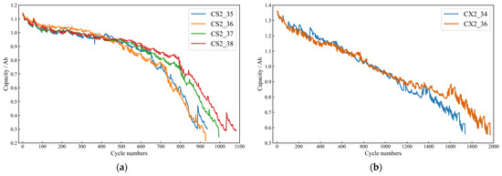
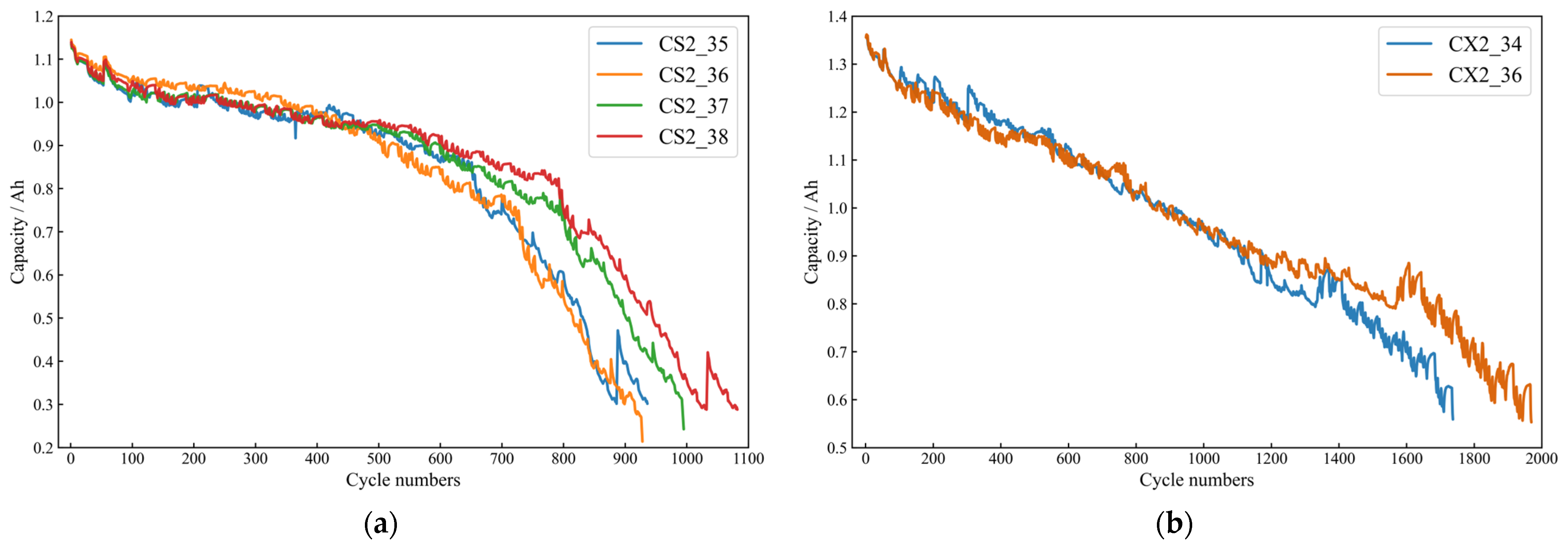
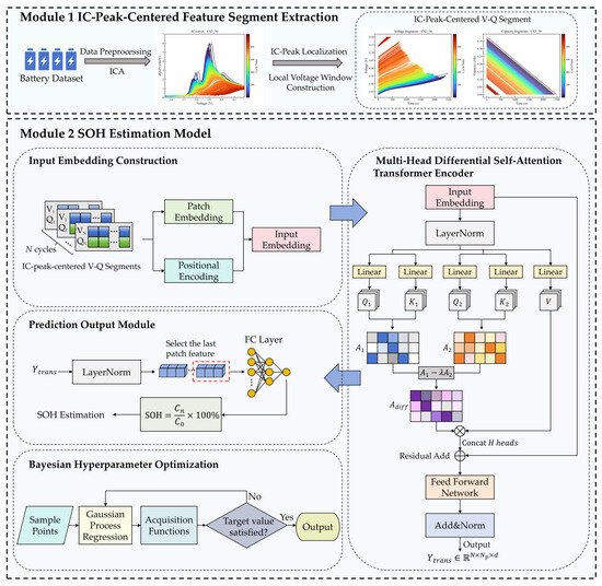
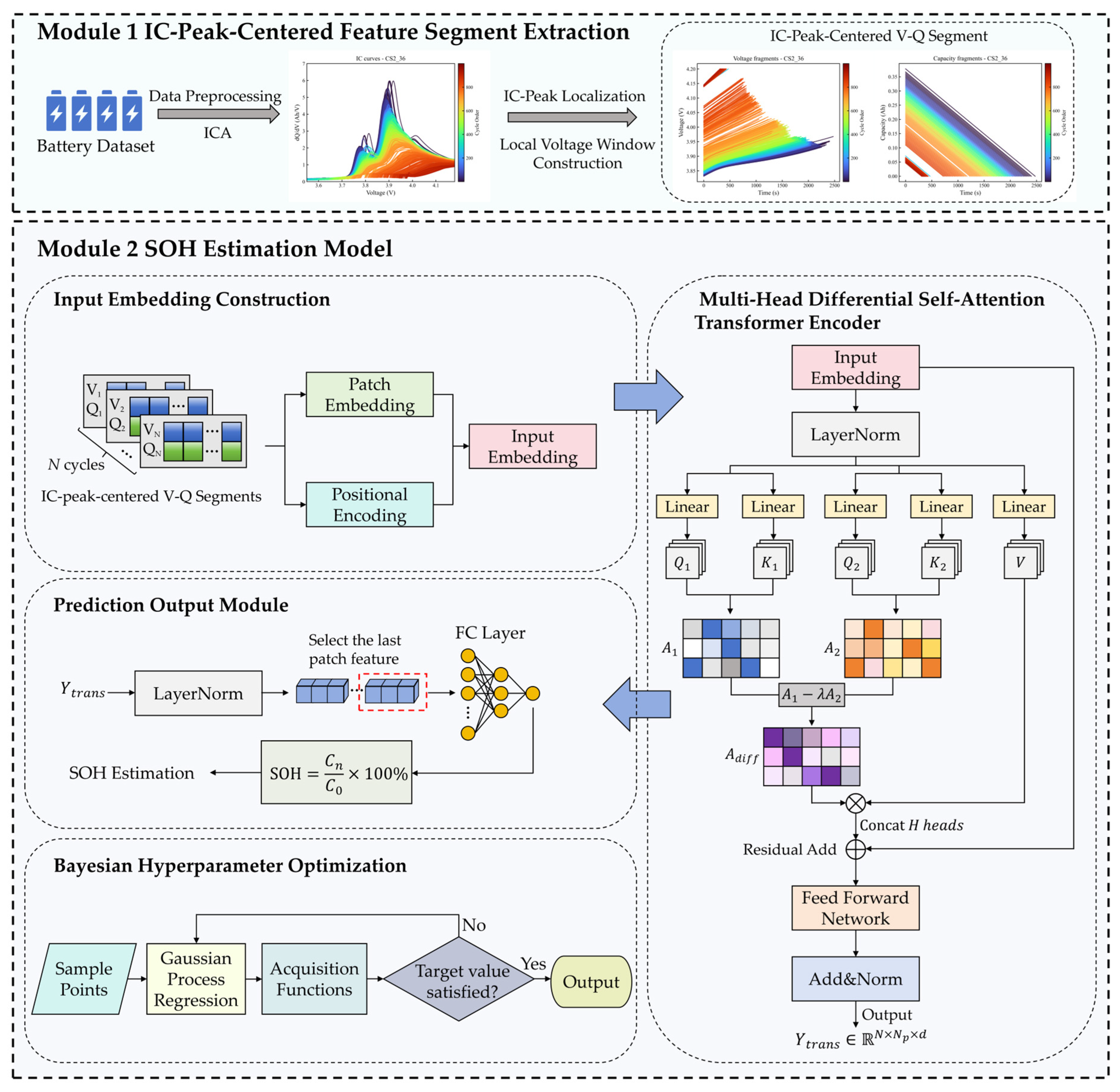
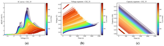
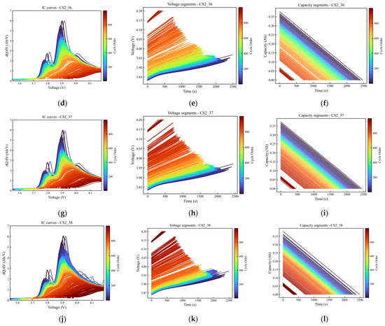
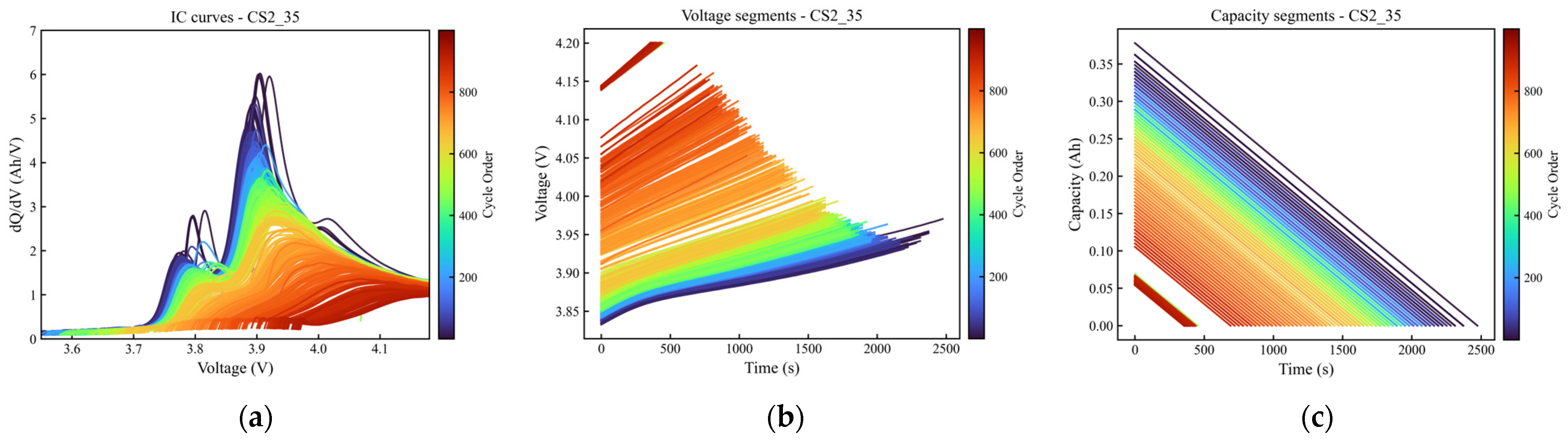
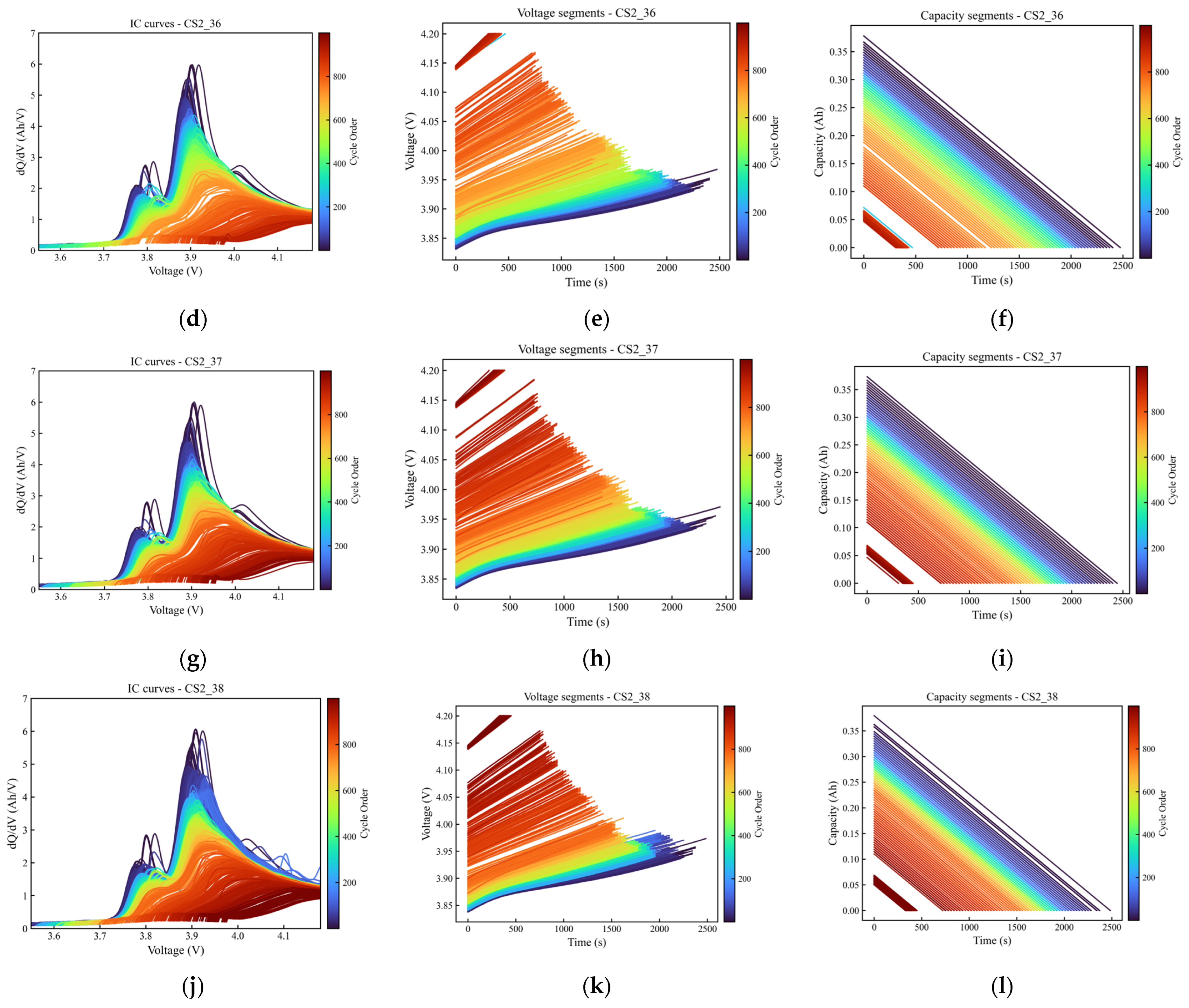
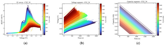
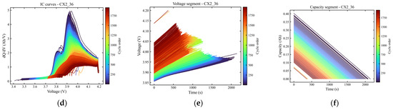
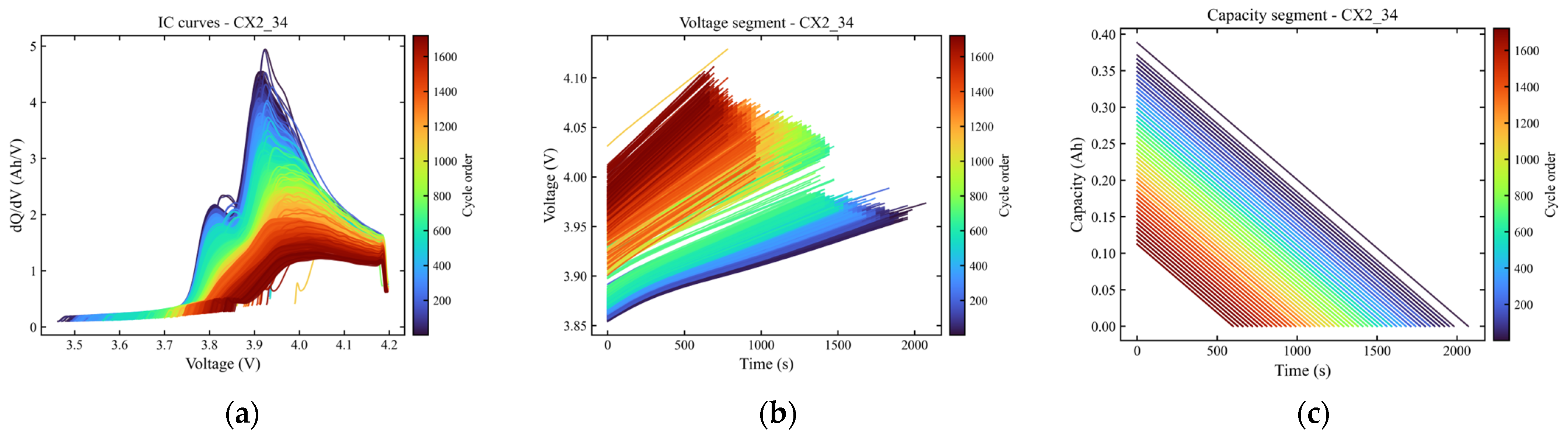
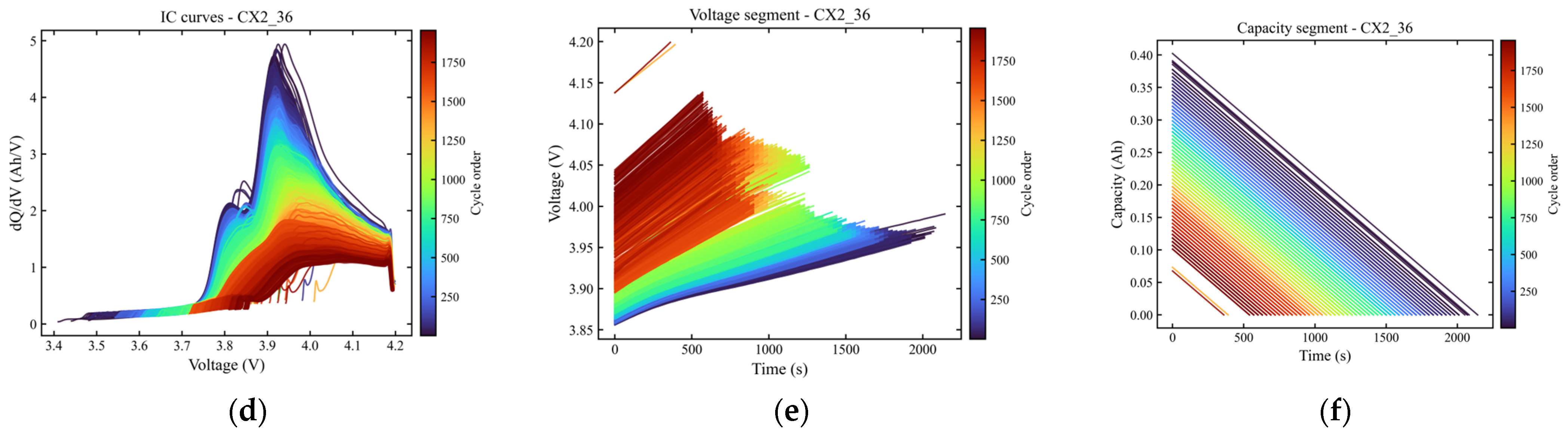
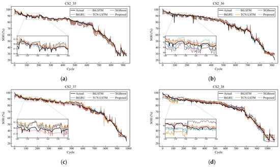
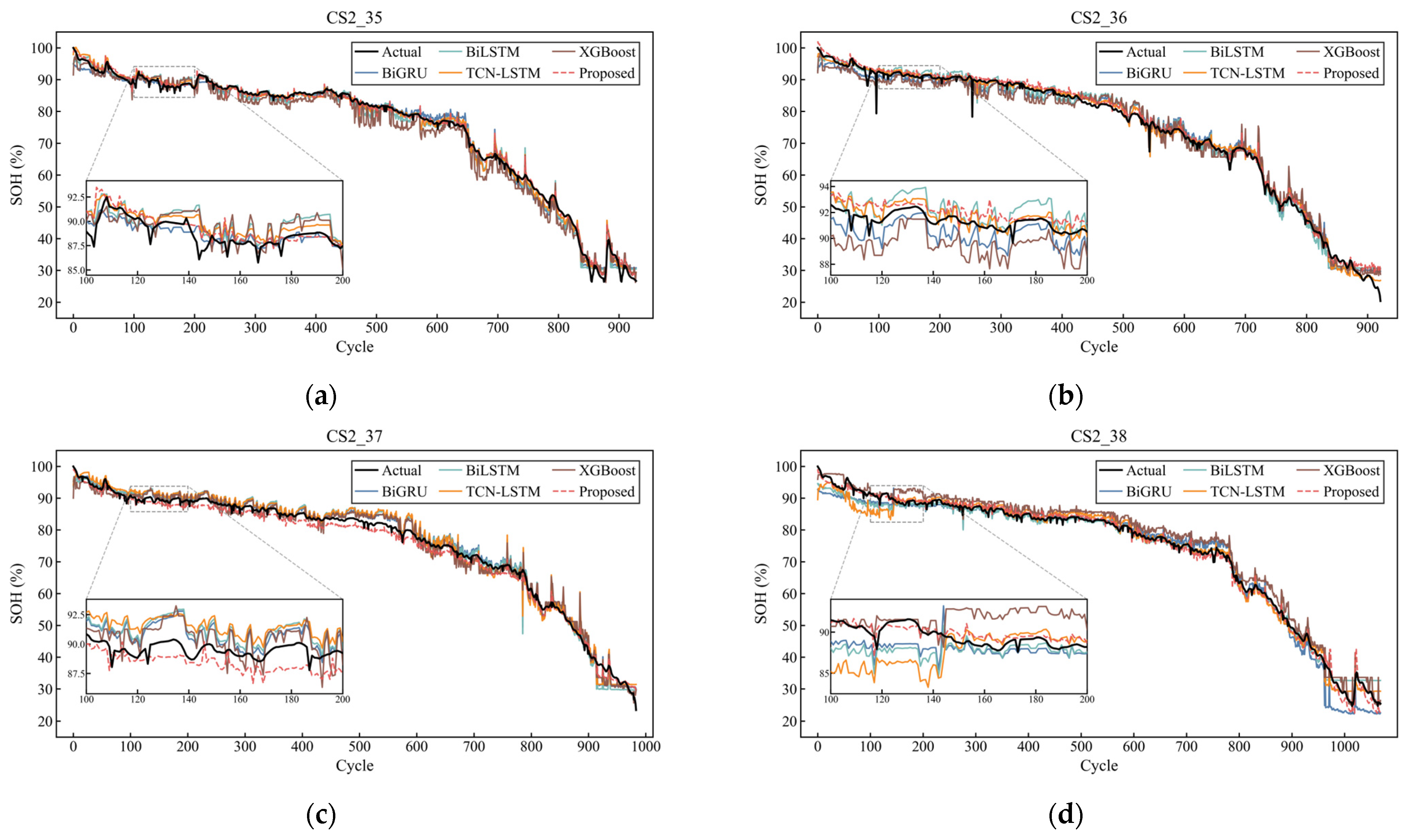
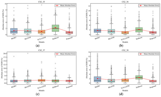
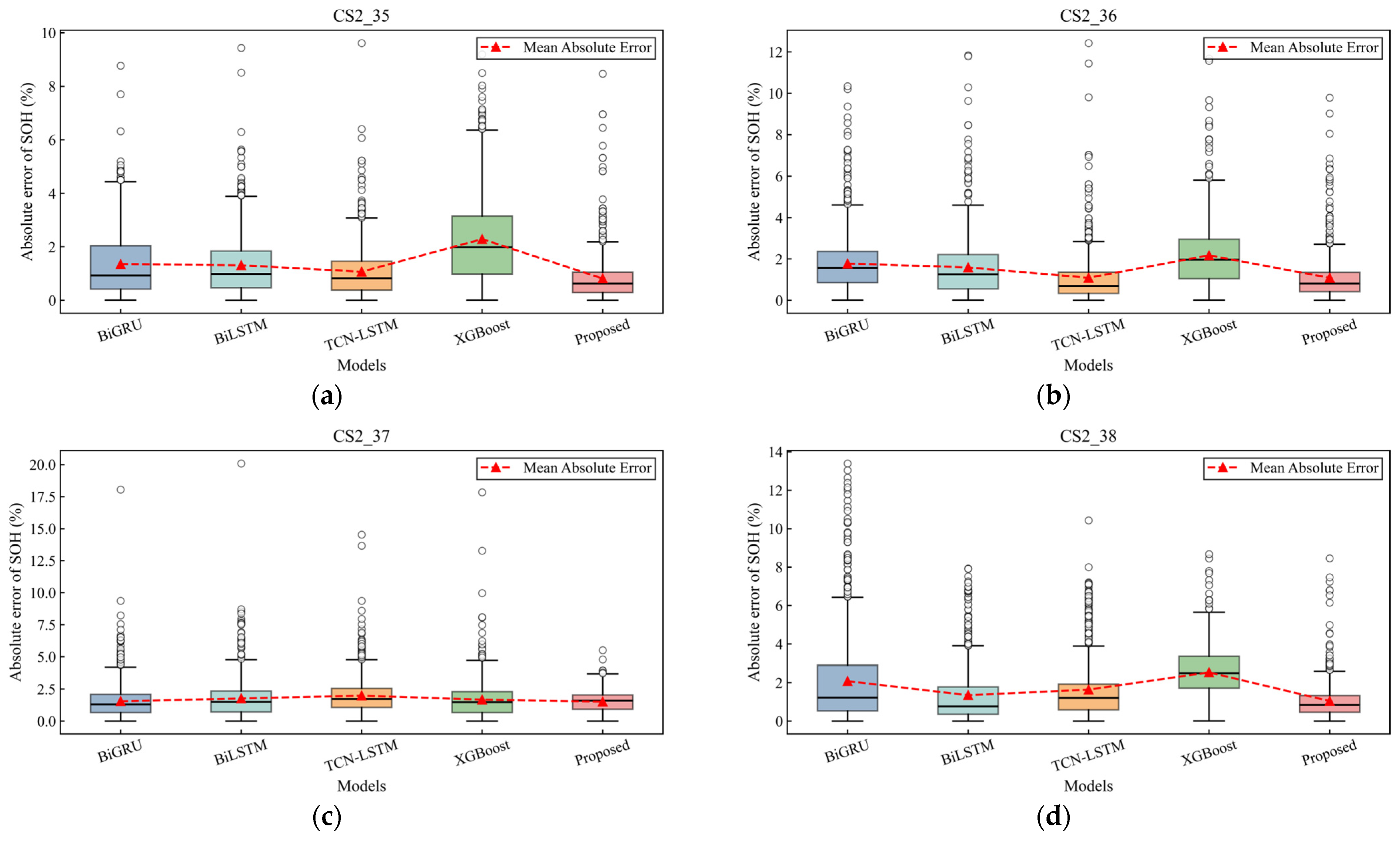
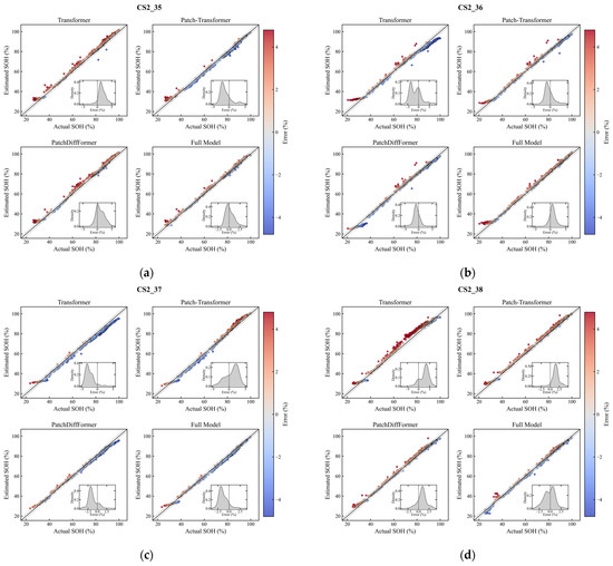
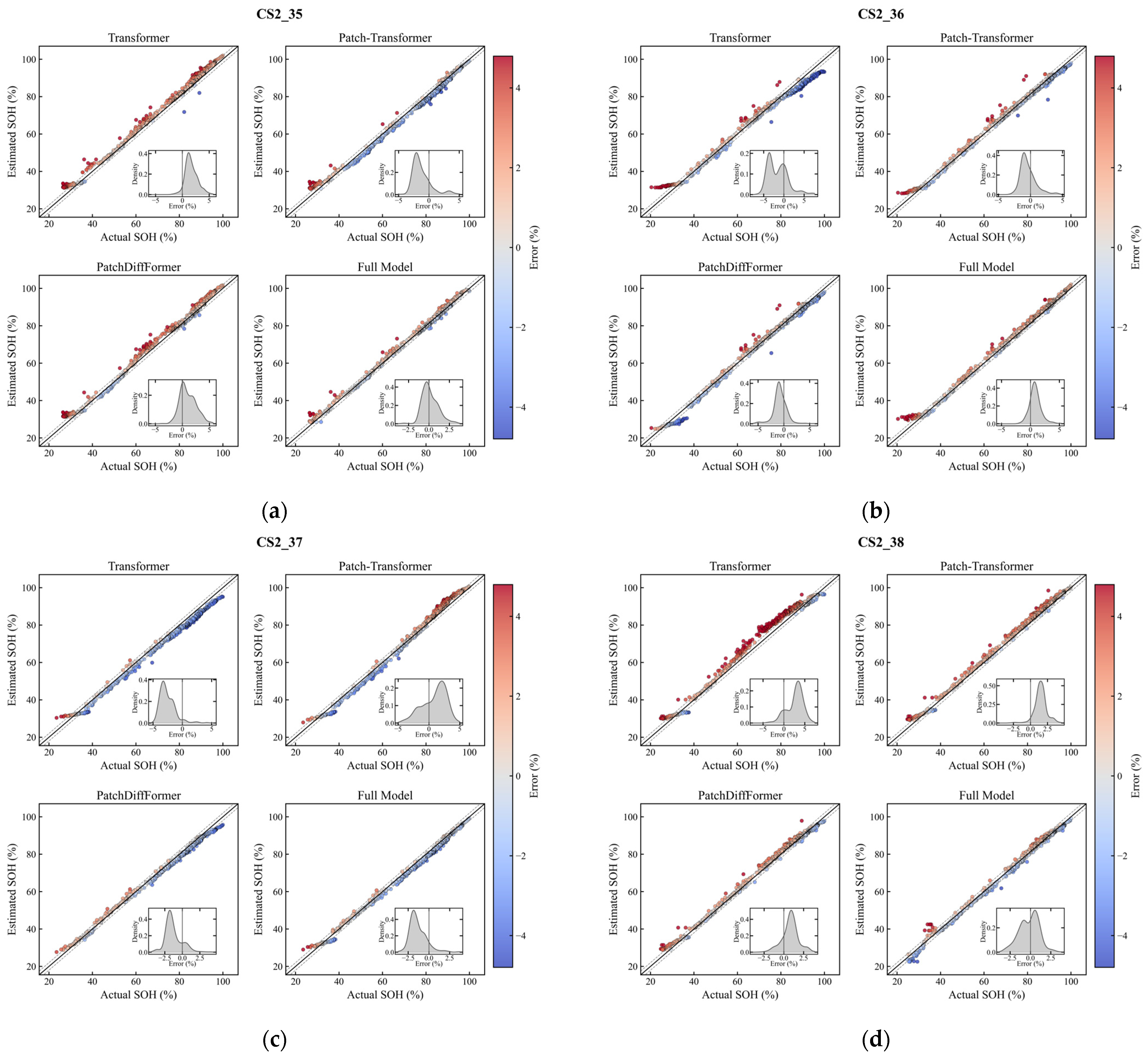
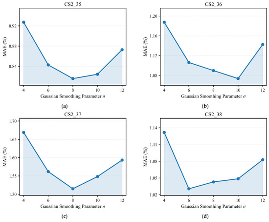
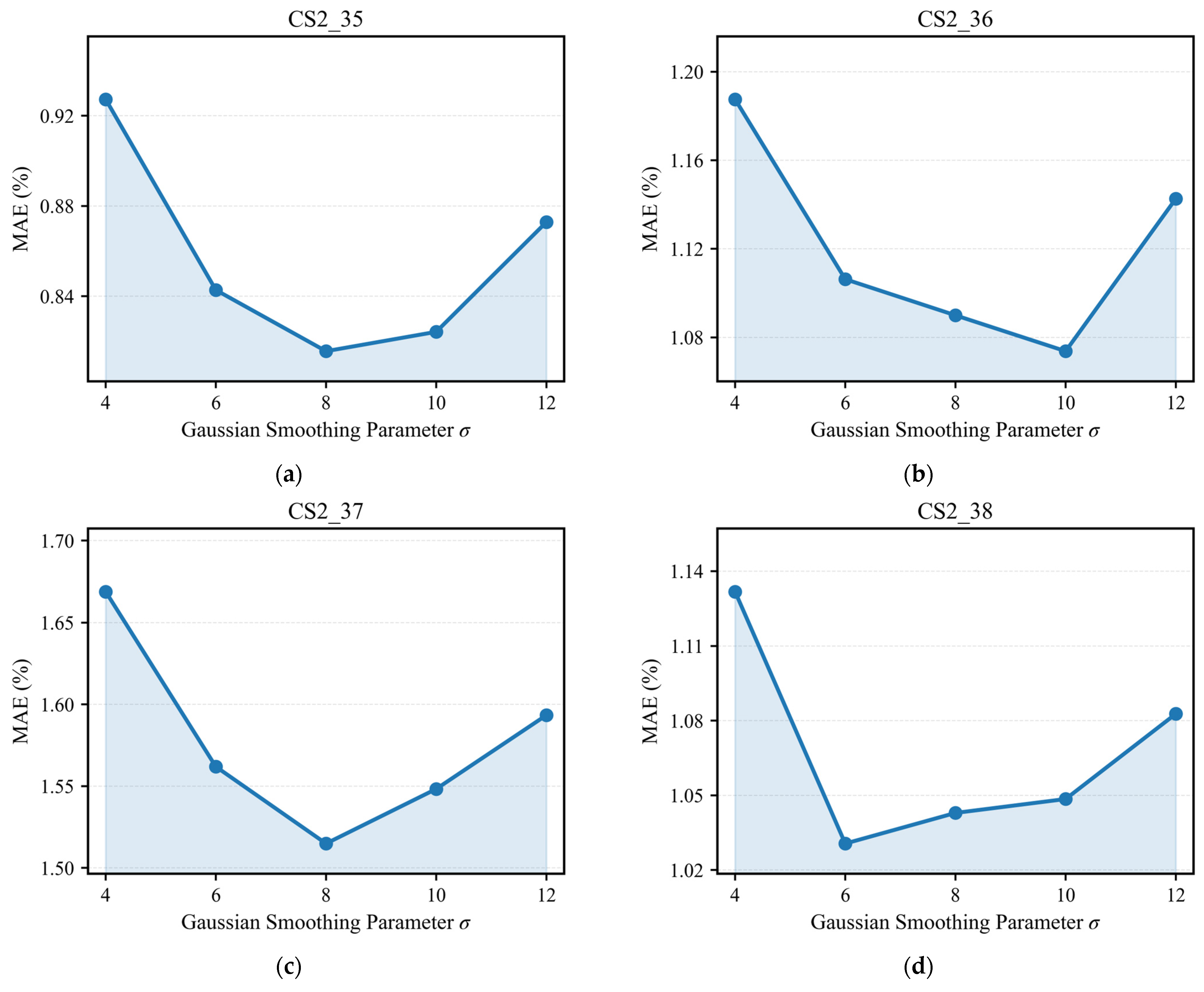
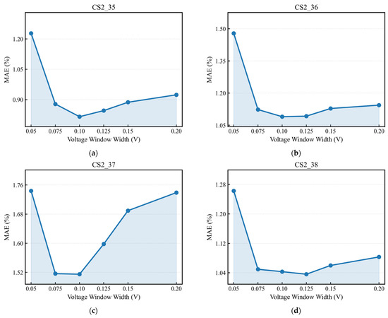
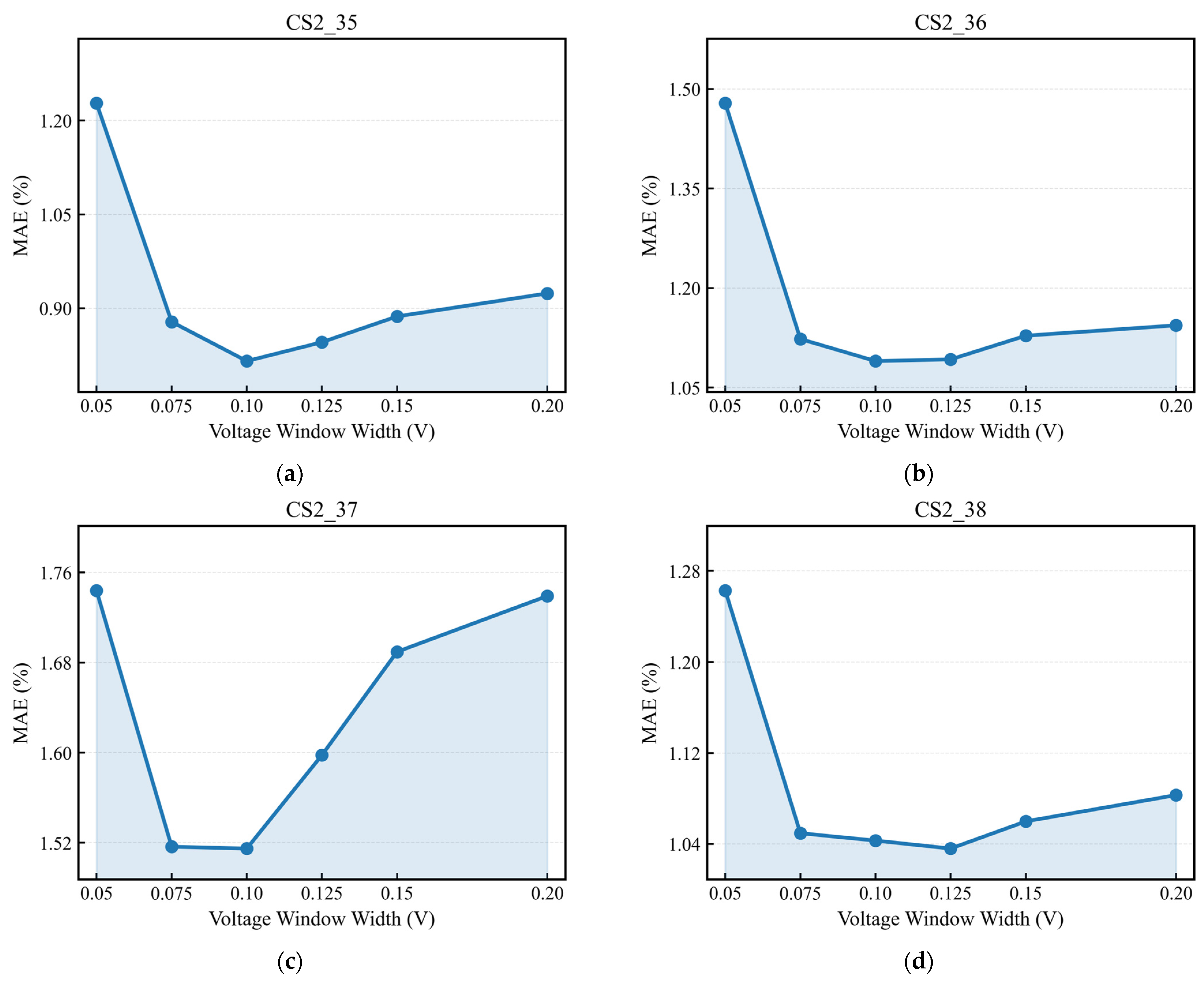
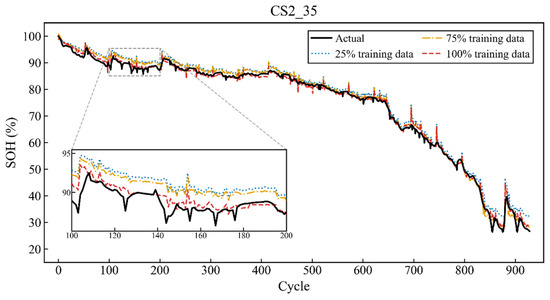
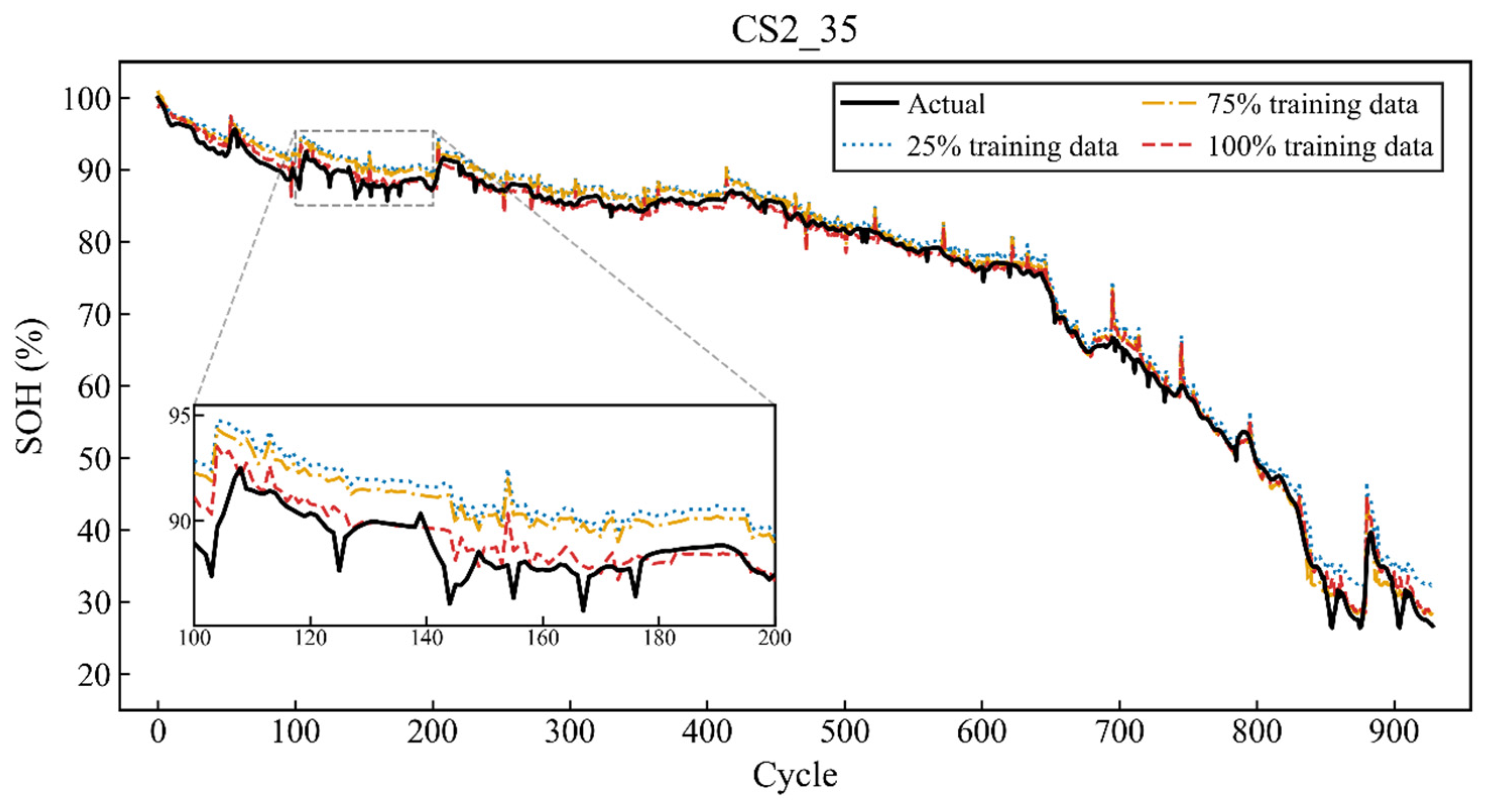
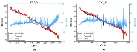
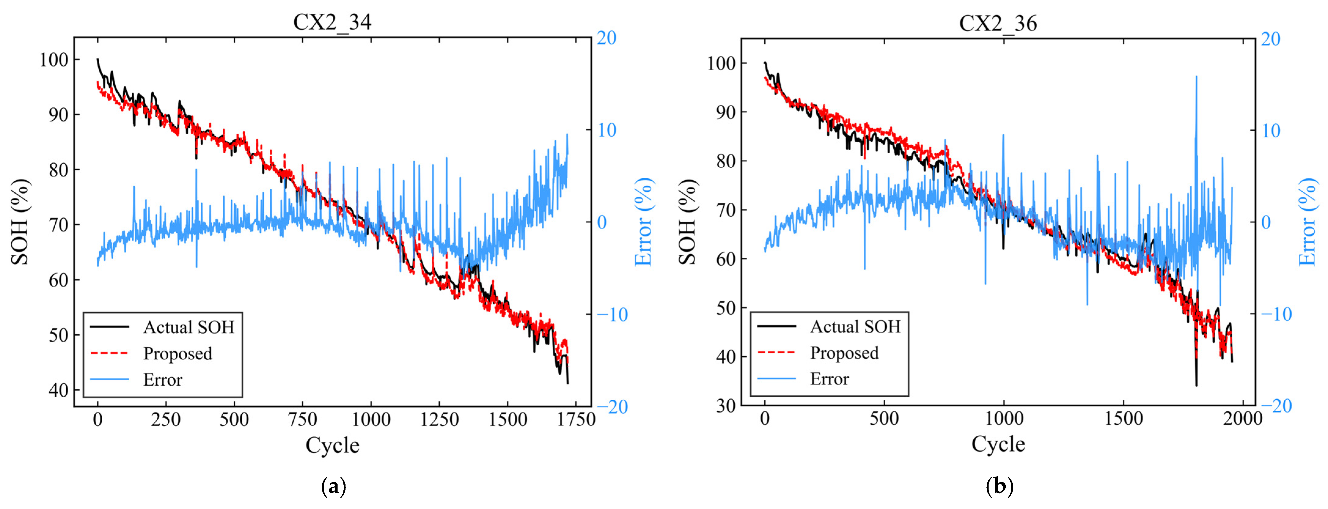

Disclaimer/Publisher’s Note: The statements, opinions and data contained in all publications are solely those of the individual author(s) and contributor(s) and not of MDPI and/or the editor(s). MDPI and/or the editor(s) disclaim responsibility for any injury to people or property resulting from any ideas, methods, instructions or products referred to in the content. |
© 2026 by the authors. Licensee MDPI, Basel, Switzerland. This article is an open access article distributed under the terms and conditions of the Creative Commons Attribution (CC BY) license.