


Abstract
Boil-off from cryogenic liquids is a significant economic, operational, and safety challenge across the global energy industry, yet existing models lack the scope and predictive capability needed to simulate boil-off across a range of fluids and storage conditions. This work introduces a new, one-dimensional lumped parameter model for predicting boil-off from a variety of fluids under a range of storage conditions. The new model divides the liquid into discrete, homogeneous layers coupled by a set of heat and mass transfer equations and can capture liquid-phase thermal stratification effects and compositional changes as the tank both self-pressurises and operates isobarically. During pressurisation, the model simulates convection within the liquid by dividing it into conduction and convection domains and calculating boundary layer and recirculation flowrates within the latter. During isobaric operation, the model applies a shortcut convection term that allows ambient heat ingress into a layer to be transferred to the liquid surface where it generates boil-off instead of heating the liquid. Unlike previously published works, this model does not require manipulation of adjustable parameters to describe pressurisation and boil-off rates relative to experimental data. It thus offers improved predictive capability compared to existing homogeneous-phase models, with applications to the design of boil-off handling systems, maritime shipping, and long-term storage of cryogenic liquids.
1. Introduction
The global energy industry faces profound change, characterised by growing energy demand alongside a need to meet this using more environmentally friendly means. Three fluids will play significant roles during this endeavour: natural gas, carbon dioxide, and hydrogen.
Natural gas is vital to the global energy mix and will continue playing a significant role for decades to come. It provides firming capacity as renewables penetration increases. Therefore, even as the world decarbonises, natural gas demand will remain robust—likely increasing—through 2050 [1]. Continued use of fossil fuels will necessitate the deployment of Carbon Capture, Utilisation, and Storage (CCUS) technologies; substantive decarbonisation will be virtually impossible without significant uptake of CCUS [2]. Hydrogen is emerging as a promising enabler of decarbonisation, and while current global production of low-carbon hydrogen is relatively small, this is projected to increase substantially by 2050 [3].
Natural gas, CO2, and H2 exist in the vapour state at typical ambient temperatures. Vapour-phase fluids are difficult to store and transport efficiently, and liquefaction is often used to significantly lower fluid volume [4]. However, liquefaction occurs at low temperatures: dewpoints at one atmosphere are −161 °C for methane [5] and −253 °C for hydrogen [6], whereas CO2 exists as a liquid only above the triple point of 0.52 MPa and −57 °C [7]. Storage at such low temperatures inevitably causes some of the liquid to evaporate, generating boil-off gas (BOG). Boil-off losses can deplete between (2–6) % of a liquefied natural gas (LNG) cargo [8]. At an industrial scale, boil-off losses require the installation of handling systems to process the gas; this is of particular concern for LNG carrier vessels, where space is at a premium.
Despite boil-off’s consequences, existing modelling attempts are of limited scope and/or predictive ability, often relying on parameters fitted to the very experiments they seek to reproduce (as discussed below). An over-reliance on empirically fitted parameters can potentially lead to inaccurate predictions, which may have hazardous or expensive consequences. A model capable of accurately simulating boil-off could thus lead to economic, operational, and safety improvements.
Here, we present a fully predictive model capable of describing boil-off, pressurisation, and thermal stratification across a range of fluids. This work makes the following novel contributions:
- During isobaric operation, the model introduces a “shortcut convection” term that transfers ambient heat ingress from a liquid layer to the liquid surface, where it generates boil-off instead of heating the liquid.
- The model resolves thermal and compositional gradients within the liquid during both self-pressurisation and isobaric operation using a single framework.
- During pressurisation, the model divides the liquid into conduction and convection domains and calculates flowrates within the latter; the thickness of the conduction domain follows from the calculated temperature profile, rather than from a correlation fitted to the experimental data. In contrast to previously published models, this model does not require case-specific tuning of adjustable parameters to reproduce the observed pressurisation rate, boil-off rate, heat transfer rates, and conduction domain thickness.
2. Literature Review
A preponderance of the published literature focuses on predicting the effect of LNG weathering, which refers to the change in the liquid’s composition caused by boil-off. Between 2008 and 2014, Dimopoulos & Frangopoulos [9] and Miana et al. [10] published models of weathering in LNG carriers, while Pellegrini et al. [11] did so for weathering in storage tanks. Their models assume vapour–liquid equilibrium but differ in the methods used to predict fluid properties, with none using reference equation-of-state (EOS) models. However, despite each model [9,10,11] representing an improvement over earlier attempts, industrial [12] and experimental [13,14] data indicate that the vapour phase in a cryogenic storage tank is at a significantly higher temperature than the liquid.
Migliore et al. [12], Huerta & Vesovic [15], and Jung et al. [16] published models that dispensed with the equilibrium assumption. Migliore et al. [12] assumed a saturated liquid and superheated vapour at constant pressure and tested it against the LNG cargo data presented by Miana et al. [10], confirming that the new non-equilibrium approach performed better than earlier models. However, Migliore et al. [12] back calculated an overall heat transfer coefficient (HTC) using a constant boil-off rate, thus only validating their mass balance and thermodynamic property predictions. Huerta & Vesovic [15] extended the model of Migliore et al. [12] to consider the vapour temperature profile. The two models disagree on the rate of vapour–liquid heat transfer; however, neither paper included a direct comparison of the model outputs with experimental data precluding assessment of their relative accuracy. Jung et al. [16] presented a model alongside experimental LNG weathering data. Their model ignored the vapour phase, assuming all heat ingress into the tank entered the liquid. It accurately predicted the change in liquid level and composition over fifty days, suggesting that most heat entering the vapour ultimately enters the liquid.
While these non-equilibrium models [12,15] represent a significant advancement over the earlier equilibrium models, they have limitations. Few data were available for testing, with Migliore et al. [12] validating their model against a single dataset. Both models employ cubic EOS models and empirical correlations for property prediction, with the former being inaccurate at LNG conditions and the latter having a limited range of applicability. Finally, as both are LNG weathering models, they were only used to simulate specific LNG mixtures over a limited range of storage conditions.
Perez et al. [13] and Al Ghafri et al. [14,17] presented the superheated vapour (SHV) model which overcomes a number of these limitations. The SHV model has the same physical basis as that of Migliore et al. [12] but dispenses with the assumption of constant pressure, allowing it to simulate a tank that first undergoes self-pressurisation before reaching a set relief pressure and transitioning to isobaric operation. The model also uses highly accurate reference EOS models, such as the GERG-2008 model for natural gas mixtures [18], to predict fluid-phase behaviour and properties.
The SHV model has seen extensive testing against boil-off data for a range of operating conditions. Perez et al. [13] and Al Ghafri et al. [14] presented the results of a series of experiments where liquid nitrogen (LN2) and LNG were boiled-off in a laboratory-scale (6.725 litre), vertical cylindrical tank; these served as validation datasets for the SHV model, which offered excellent reproductions of pressurisation time and average boil-off rate for both fluids. Further testing against data from an LNG weathering test conducted at Kennedy Space Centre [17] demonstrated the SHV model’s suitability for simulating LNG boil-off and weathering.
The SHV model is not fully predictive, as it relies on three adjustable parameters: the vapour–ambient, liquid–ambient, and vapour–liquid heat transfer coefficients. For a well-insulated tank, the dominant contribution to the first two is the insulation. However, an average vapour–liquid HTC was determined solely by fitting to experimental data, capturing all interphase heat transfer effects in a single parameter. Moreover, as heat transfer between different fluid phases depends on their respective properties, assuming a constant value may be invalid, particularly as a tank pressurises or liquid composition changes.
These models [9,10,11,12,13,14,15,17] also contain a major simplification: the assumption that phases are homogeneous. All assumed an isothermal liquid, while all but two [12,15] assumed the same for the vapour. However, the data reported for LN2 [13] and LNG [14,17] indicate that temperature gradients exist within the liquid, particularly as a tank pressurises, and within the vapour regardless of operating mode. These effects can be ignored for LNG weathering predictions, as this occurs in a near-isothermal LNG cargo. However, resolution of liquid-phase thermal stratification is a requirement for simulating transient pressure and dynamic boil-off behaviour. An isothermal, saturated liquid assumption causes underprediction of pressurisation time, because maintaining the whole liquid at a (higher) saturated temperature will consume ambient heat that would otherwise generate boil-off in a model which allows some of the liquid to be subcooled.
Daigle et al. [19], Wang et al. [20], and Kim et al. [21] presented different approaches to accounting for stratification. Daigle et al. [19] developed a model where each layer is divided into control volumes representing a boundary layer along the tank wall and the bulk fluid elsewhere; mass flow between adjacent elements accounts for convection. Their model predicted the formation of temperature gradients in an initially isothermal LH2 system, but they did not validate their model using experimental data despite their predictions being qualitatively correct. Wang et al. [20] also presented a model which includes the convection boundary layer, but they divided the liquid into conduction and convection domains, with the boundary layer only existing in the latter (consistent with experimental observations [22]). They validated their approach against experimental data for LN2 measured by Perez et al. [13]; however, their model is not fully predictive, relying on adjustable parameters to calculate the boil-off and vapour–liquid heat transfer rates and the thickness of the conduction domain. Kim et al. [21] proposed a model which resolved the boundary layer by integrating its momentum and energy equations and validated it using experimental data for different liquid fill levels. Accounting for liquid-phase thermal stratification yielded significantly better pressurisation rate predictions, and they employed a more rigorous treatment of the boundary layer. However, their approach is significantly more complex, and solutions to the boundary layer equations are specific to a system geometry and associated set of assumptions.
Taken together, these works illustrate two persistent limitations. The first is scope: many models make assumptions which limit their applicability to specific scenarios. The second is a reliance on empirically fitted parameters. Models that reproduce measured pressurisation rates, boil-off rates, and conduction domain thickness by tuning coefficients against the same experiments cannot be assumed to hold for other fluids, tank geometries, and operating conditions. Such over-reliance can lead to inaccurate predictions, which may have hazardous or expensive consequences: boil-off handling systems sized against an underpredicted rate may prove inadequate, while overprediction will impose additional capital costs.
3. Model Description
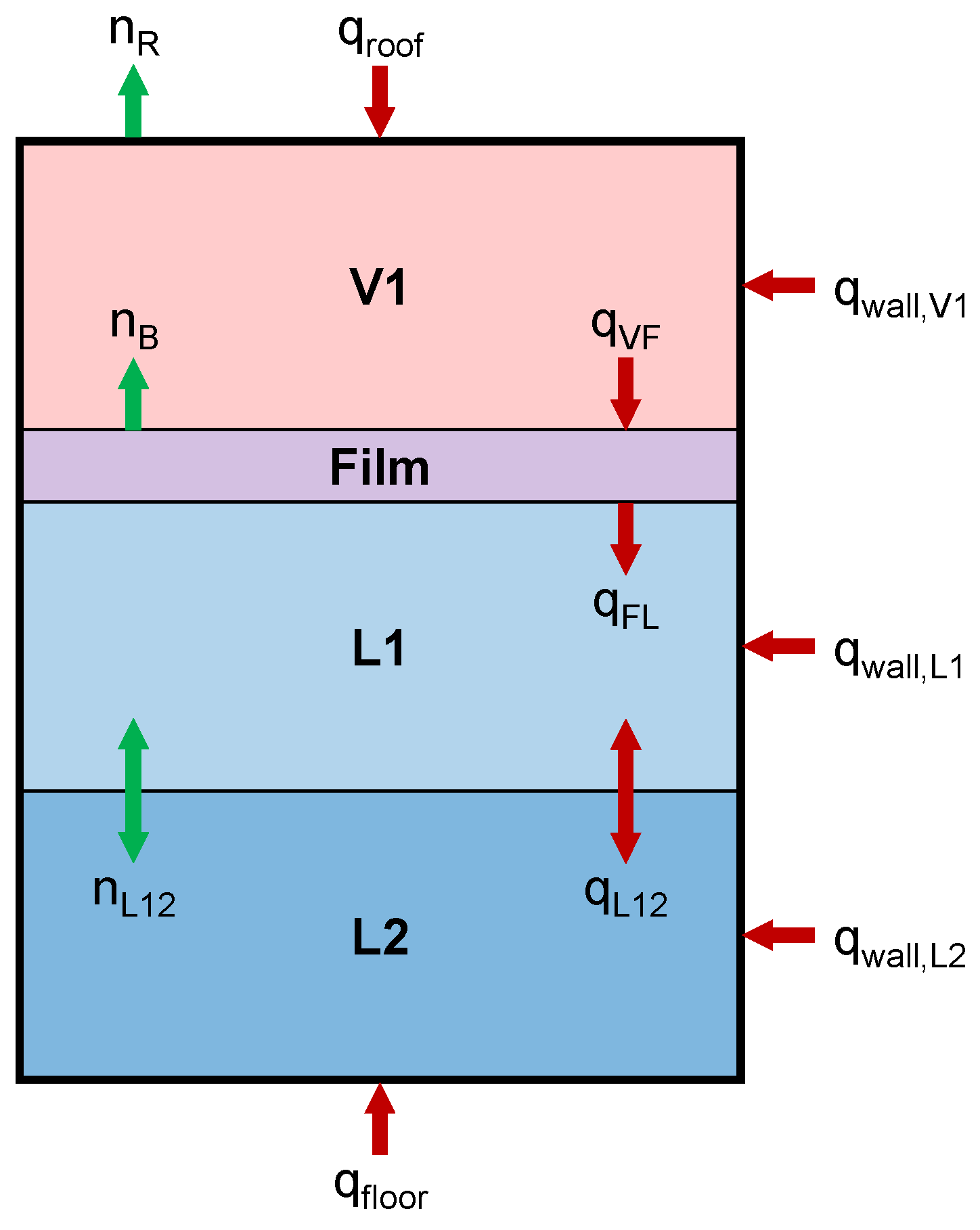
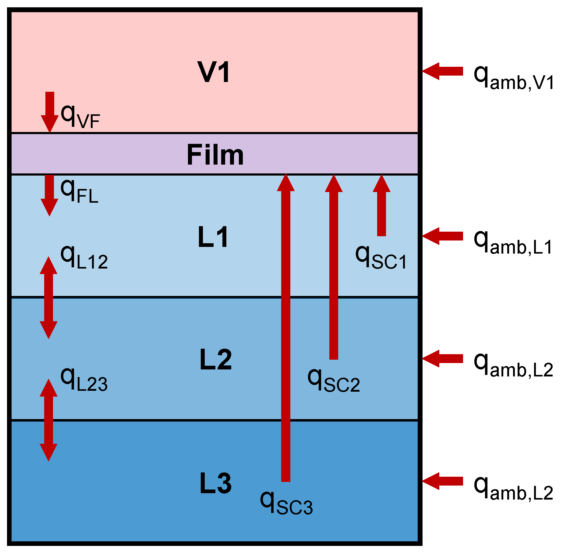
This work introduces a new boil-off model that can be adapted to simulate a range of scenarios while relying on minimal adjustable parameters. The model uses a one-dimensional lumped parameter approach illustrated in Figure 1: a tank contains vapour and liquid separated by a film of saturated liquid, with heat and mass exchange between layers and with the ambient environment. For illustration, Figure 1 contains a single vapour layer and two liquid layers; the model imposes no such requirements on either phase. The model assumes the following:
- In the spatial domain, the vapour and liquid phases are divided into any number of layers, each of which is of homogeneous pressure, temperature, and composition.
- A simulation is divided into discrete timesteps. Layer properties are known at the start of a step and calculated for the end of the step. The model does not resolve changes in properties during a step.
- Multiple phases may not exist in a single layer.
- The ullage is of uniform pressure, while liquid pressure increases with depth. The pressure of a liquid layer is that at its midpoint.
- The initial vapour composition is that of the incipient vapour at the uppermost liquid layer’s bubble point.
- Layers of a given phase are of equal volume. Should volumes become unequal during a step, a “remeshing” procedure is applied.
- An infinitesimally thin film of saturated liquid is located atop the bulk liquid surface. No mass or energy accumulates within the film.
- The film has a pressure equal to the ullage and a composition equal to that of the uppermost liquid layer.
- Boil-off gas evolves from the film and has composition and properties equal to that of the incipient vapour at the film’s bubble point.
- The tank can undergo pressurisation or operate isobarically.
- During pressurisation, no material enters or leaves the tank, but material exchange between phases can occur.
- During isobaric operation (the relief stage), the tank vents vapour to maintain a constant ullage pressure.
- All layers except the film undergo ambient heating by steady-state conduction through the tank.
- Heat transfer between adjacent layers of the same phase is by conduction if the upper layer is hotter and convection otherwise.
- Vapour layers typically become superheated after the start of a simulation, whereas liquid layers are typically subcooled. A liquid layer can become saturated with sufficient heat ingress into that layer.
- If, within a single step, the total heat ingress into a liquid layer exceeds that required to saturate it, the excess heat is transferred to the film via a mechanism termed here as “shortcut” convection.
- Convection within the liquid can be accounted for using a shortcut method or by calculating convective circulation rates. In the latter case, there is no net change in the amount of liquid in each layer that undergoes convective circulation.
- All interphase mass transfer occurs between the layers on either side of the film due to boil-off or condensation.
- In mixtures, interlayer mass transfer occurs due to concentration gradients between adjacent layers.
Figure 1.
A tank containing vapour (in layer V1) and liquid (in layers L1, L2), with a film of saturated liquid located between them. This figure exaggerates film thickness: the model assumes it to be zero. Red arrows represent heat transfer, and green arrows represent mass transfer.
4. Overview of the Algorithm
The model is implemented using modern Fortran [23] due to its high performance and suitability for scientific computing. A freely available Windows application, BoilFAST 2, is available for simulations using this model [24]. It consists of a high-level “driver” algorithm and a low-level simulation step algorithm. The driver interfaces with the user and controls a simulation thus:
- The user provides sufficient data to fully describe the tank geometry, thermodynamic state of fluids within the tank, and heat ingress from the ambient environment as a function of time.
- All unspecified fluid and layer properties are calculated. For example, if the user has provided an initial ullage pressure and liquid composition, the driver performs a bubble point flash to determine film and liquid temperatures and calculates unknown layer fluid properties using an EOS model.
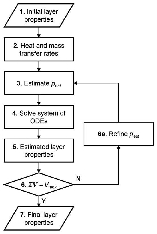
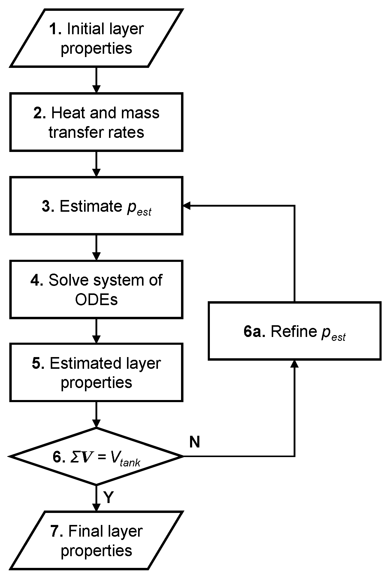
- The driver takes a simulation step using the low-level algorithm outlined in Figure 2.Figure 2. Simulation step algorithm used to calculate layer properties at the end of a timestep given the initial properties.
- If required, the driver performs remeshing to equalise layer volumes within a phase.
- The driver validates the simulation step solved in Step 3 according to the criteria below. If a criterion is not met for reasons related to numerical tolerance, the simulation is terminated.
- The total volume of the vapour and liquid phases should equal the tank volume.
- The total amount of each chemical species at the end of the step should equal the initial amount, less the amount of that species in the relief vapour.
- The total enthalpy of the fluid at the end of the step should equal the initial enthalpy, plus heat ingress from the ambient environment during the step, less the enthalpy of the relief vapour.
- If the current simulation time is not equal to the maximum simulation time, the simulation advances by a timestep, repeating Steps 3 through 5.
- Upon reaching the maximum simulation time, the simulation ends, and the driver returns the results to the user.
The model uses a lower-level simulation step algorithm (Figure 2) to advance a simulation by one timestep. The algorithm calculates all layer properties at the end of a timestep given their initial values according to the following:
- The initial values of all layer fluid and geometric properties are specified.
- The algorithm calculates initial heat and mass transfer rates. This includes all ambient and interlayer heat transfer rates, the boil-off rate, and where relevant, the rates of convective and diffusive mass transfer.
- If the tank is pressurising, the algorithm estimates the ullage pressure at the end of the step.
- Knowing the initial rates of heat and mass transfer, the algorithm solves a system of ordinary differential equations (ODEs) for the enthalpy and molar amount of each chemical species in each layer at the end of the step, as detailed below.
- Having determined the enthalpy and composition of each layer by solving the ODEs, the algorithm calculates estimated fluid properties for each layer by solving a series of p-h flashes.
- If the total of all estimated layer volumes is not equal to the tank volume, the algorithm either refines the estimated pressure using the Newton–Raphson method and repeats Steps 3 through 6 if the tank is pressurising or calculates the required vapour relief rate if the tank is operating isobarically.
- Upon convergence of total layer volume with tank volume to within a user specified tolerance, the algorithm completes the current step and returns the final layer properties to the driver algorithm.
4.1. Heat Transfer
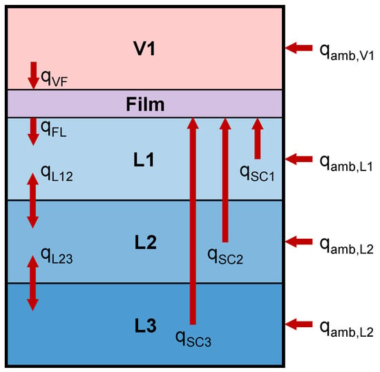
Figure 3 outlines the three categories of heat transfer considered by the model. For ambient heating and interlayer heat transfer, the model calculates the heat transfer rate, q, using the temperature difference, ΔT, the heat transfer area, A, and a heat transfer coefficient, , predicted from the relevant fluid properties:
Figure 3.
Categories of heat transfer considered in the model: ambient heat ingress into each layer (amb), interlayer heat transfer (VF, FL, L), and shortcut convection (SC).
All calculations use the known layer fluid properties and geometry at the start of the current step.
Ambient heating is defined by specifying the ambient temperature and an overall heat transfer coefficient between the fluid inside the tank and the surrounding environment. The model then solves Equation (1) for each layer, using the layer and ambient temperatures to calculate .
Conductive heat transfer between two adjacent layers within the same fluid phase is also found using Equation (1); however, the heat transfer coefficient is first found thus:
where λ is the average thermal conductivity of the two layers, and x is the distance between the layer midpoints. To calculate vapour–liquid heat transfer, the above formula is used to calculate between the film and liquid, while the McAdams correlation [25] is used for vapour–film heat transfer:
where Ra is the Rayleigh number and is the Nusselt number, which is related to the heat transfer coefficient thus:
Any convective heat transfer between adjacent fluid layers in the same phase is accounted for by evaluating the enthalpy associated with the convective mass flow. This flow is calculated using correlations detailed in the section on mass transfer below; they implicitly require the lower-layer temperature to exceed that of the one above.
The model applies a shortcut convection mechanism to each liquid layer as it is about to reach its saturated temperature, transferring heat directly to the film regardless of the layer’s location. The rate of shortcut convection is set equal to the rate of ambient heat ingress into the layer (to avoid it boiling): thus, when this convective term is applied to a liquid layer, the ambient heating generates extra boil-off gas instead of heating that layer. Regardless of where shortcut convection applies, the extra boil-off gas it produces evolves from the uppermost liquid layer. Shortcut convection differs from convective circulation in that no associated mass transfer occurs.
The physical basis for this shortcut lies in the disparity between the timescales of convective transport and of ambient heating. Scurlock [26] describes how, in a real system, convection currents carry heat absorbed anywhere within a cryogenic liquid to its surface, superheating the region beneath the vapour–liquid interface and thereby driving boil-off production. During isobaric operation, convection is rapid, and a model which shortcuts heat directly to the film will yield the same net outcome as one which transfers it very rapidly.
Existing convection correlations do not achieve this outcome. When correlations such as those of Globe & Dropkin [27] are applied, heat is not transferred to the liquid surface in sufficient quantity to prevent the lowermost liquid layer first reaching saturation and vaporising, a behaviour which is not observed experimentally and which would place boil-off production at the bottom of the liquid rather than at its surface. Shortcut convection enforces the physically correct destination for the ambient heat, even though it does not resolve the specific transport mechanism.
This approach reproduces the destination of the heat rather than the mechanism by which it arrives. In a real system, the liquid beneath the surface superheats [26], and this superheat is the immediate driver of boil-off. Predicting the degree of such superheating is inherently difficult for a model based on thermodynamic calculations. Shortcut convection is therefore an approximation which reproduces the boil-off rate without simulating the superheated liquid responsible for it.
If a liquid layer is already saturated, the model uses a modified shortcut convection term, which equals the rate of excess heating above that required to maintain the liquid enthalpy at its saturated value. This can include ambient heat ingress and heat entering from an adjacent layer; in the case of mixtures, this also includes “quasi-heating” occurring when compositional changes reduce the saturated liquid enthalpy below the current layer enthalpy.
4.2. Mass Transfer
4.2.1. Boil-Off Rate
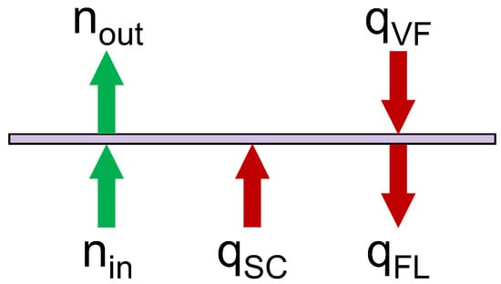
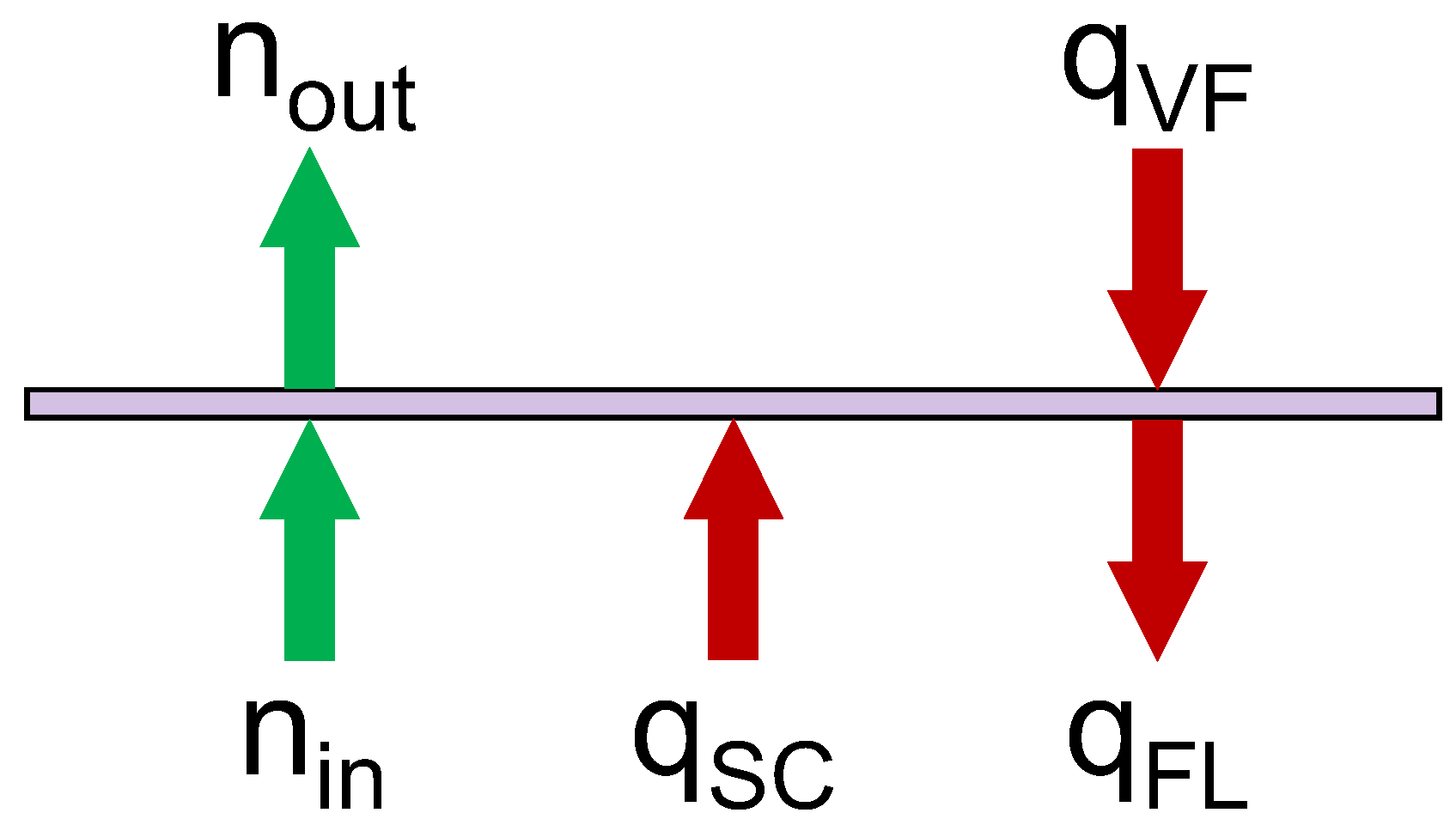
Solving an energy balance on the film, shown in Figure 4, gives the boil-off (or condensation) rate.
Figure 4.
Energy balance on the film. Red arrows show heat transfer and green arrows show mass transfer: qVF is heat entering the film from the vapour, qFL is heat leaving the film for the liquid, and qSC is the shortcut convection term.
As the film is infinitesimally thin, it has no volume; consequently, mass and energy cannot accumulate therein:
It follows that mass transfer through the film is at steady state:
Heat flows affecting the film include vapour–film heat transfer qVF, film–liquid heat transfer qFL, and the total shortcut convection from all liquid layers qSC. The net heating experienced by the film is the following:
As energy cannot accumulate in the film, qin must be balanced by the enthalpy of vaporisation of the boil-off gas. Thus, the boil-off rate equals the following:
where is the enthalpy of the boil-off gas, equal to that of the incipient vapour at the film bubble point, and is the enthalpy of the uppermost liquid layer. This is used instead of the saturated (film) liquid enthalpy as the liquid in this layer is the source of the boil-off and must thus be first heated to its saturated enthalpy before it can evaporate. If the numerator is negative, excess heat is leaving the film for the liquid and condensation occurs; Equation (8) becomes the following:
where is the enthalpy of the liquid film, and is the enthalpy of the m-th (lowermost) vapour layer.
4.2.2. Stability Ratio
For mixtures such as LNG, it is possible that two liquid layers might approach hydrostatic instability because of the different effects of heat and mass transfer on the layer’s density. Such an instability can lead to a rollover event [28]. Accordingly, the model calculates the hydrodynamic stability ratio, RS, between a pair of adjacent liquid layers j and j + 1 thus [28]:
where ρ is the mass density, and β is the coefficient of thermal expansion; an overbar denotes the average value of that property for the two layers. The model uses the specified EOS to compute the mass density of each layer at the start of every timestep given its temperature and composition. Thus, it tracks the evolution of the stability ratio for all pairs of adjacent liquid layers during a simulation.
4.2.3. Interlayer Diffusion
When simulating boil-off from a mixture, the model will calculate rates of diffusion mass transfer between adjacent layers in the same phase. This process is analogous to heat transfer and solved similarly: the model first calculates MTCs for each fluid component by applying either the Reynolds or Chilton–Colburn analogies to the interlayer HTC, before calculating the diffusion rate.
The model selects the appropriate mass transfer analogy, based on the stability ratio. Arjomandnia et al. [28] deduced a critical stability ratio of 3.8: below this value, convection dominates the system and the Reynolds analogy holds, while above this value, the Chilton–Colburn analogy holds. The latter requires knowledge of the diffusion coefficient of each component in the mixture, Di, found using a correlation presented by Pickering [29]:
where N is the number of components in the fluid, xj is the mole fraction of component j, and Dij is the binary diffusion coefficient of species i in solvent j, calculated thus:
where η is the dynamic viscosity of solvent j, kB is the Boltzmann constant, T is the fluid temperature, σ is the Lennard–Jones collision diameter and M the molar mass of a component.
4.2.4. Convective Mass Transfer
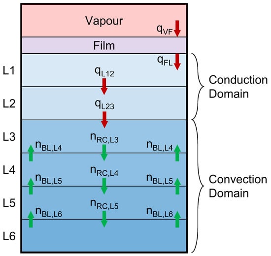
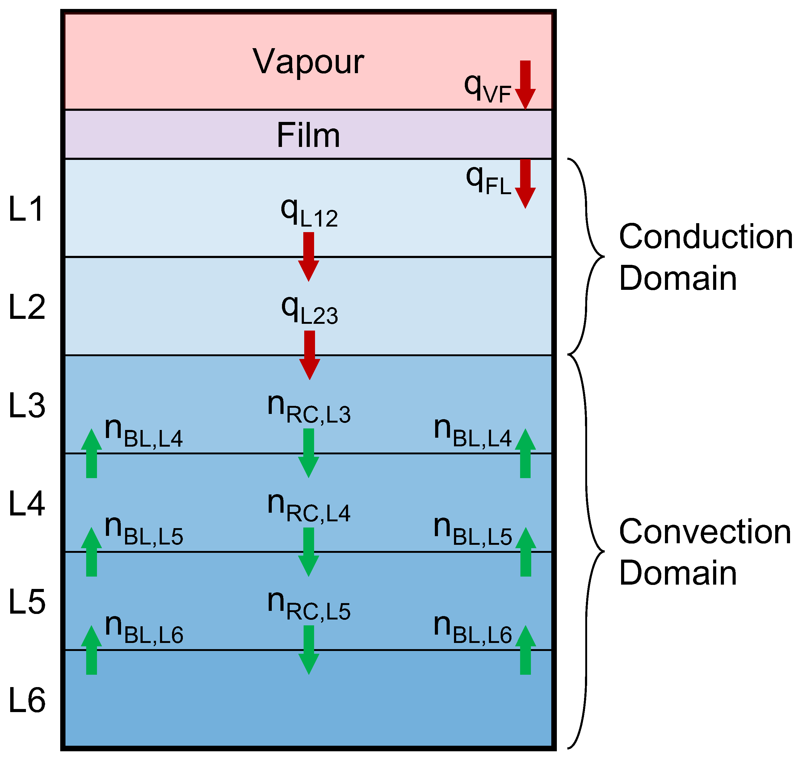
During the pressurisation stage of a simulation, the model calculates convective circulation rates within the liquid phase, illustrated in Figure 5. This approach sees the liquid divided into a conduction domain below the film, where no circulation occurs, and a convection domain in which liquid circulation occurs. The conduction domain is defined as the volume of liquid in which, for any two adjacent layers, the hotter layer is on top; in practice, this results in the conduction domain extending from the film to the coldest liquid layer. This is consistent with some experimental studies [22], which indicate that the liquid contains a thermally stratified zone immediately beneath the film and a well-mixed near-isothermal zone elsewhere.
Figure 5.
A tank containing a liquid phase divided into conduction and convection domains. Red arrows represent interlayer heat transfer, and green arrows represent liquid flows caused by convective circulation.
During pressurisation, the saturated temperature at the vapour–liquid interface rises with the ullage pressure faster than the bulk liquid temperature can increase. Consequently, temperature gradients develop within the liquid, and the resulting convection must be resolved. In contrast, during the isobaric (relief) stage, the interface is held at a fixed temperature, and all heat absorbed by the liquid is transported to its surface, driving boil-off production. The model therefore calculates convective circulation only during the pressurisation stage and accounts for heat flows within the liquid during isobaric operation using shortcut convection.
Within the convection domain, a boundary layer forms near the tank wall, transporting fluid upwards, while a plume in the middle of the tank recirculates the liquid. The recirculation rate across a layer–layer interface is equal in magnitude but opposite in direction to the boundary layer flow. Therefore, circulation causes no net change in the amount of liquid in a layer but can change its composition if adjacent layers are of different composition. The model calculates flowrate in the boundary layer by first solving for its thickness δ and the average upward flow velocity u therein. Kakaç et al. [30] give the following equations for a laminar boundary layer:
For a turbulent boundary layer, Eckert & Jackson [31] give the following:
where x is the boundary layer height—here, taken as the height of the layer midpoint above the tank floor—while ν is the kinematic viscosity, Pr is the Prandtl number of the fluid in the boundary layer, and Gr its Grashof number:
Here, ΔTFW is the temperature difference between the fluid and the tank wall, which the model calculates iteratively given the Raithby & Hollands correlation for convection near a vertical wall [32]:
The model selects the appropriate set of laminar or turbulent boundary layer correlations using the Rayleigh number, Ra, with a laminar–turbulent transition occurring at the following:
Having found the thickness and flow velocity, the vertical molar flowrate in the boundary layer follows thus:
Here, C is a coefficient, equal to 0.0833 for a laminar boundary layer and 0.1436 for a turbulent one [33], and ρ is the molar density of the fluid.
Tellep & Harper [34] presented empirical correlations for the conduction domain growth rate, which were used by Wang et al. [20] with the addition of a time adjustment factor to fit experimental data. However, when tested with our model, the Tellep & Harper correlations [34] returned unphysical conduction domain thicknesses. To avoid introducing adjustable parameters, the conduction domain is determined in this work as an output of the model, defined as the region of the liquid between the film and the coldest liquid layer.
4.3. System of Ordinary Differential Equations (ODEs)
The enthalpy and amount of each chemical species in a layer j at the end of the current step are given by:
where H is the total layer enthalpy, X is a vector of the total amount of each chemical species in the layer, and Δt is the step length. The subscript 0 denotes the start of the current step, and 1 denotes the end. The derivative of the layer enthalpy is the following:
where qtop, qwall, and qbot are the heat ingress through the layer top, walls, and bottom, qSC is the heat transferred to the film by shortcut convection, and ΔHn is the net change in enthalpy associated with the addition and removal of fluid to/from the layer, given by the following:
where is the molar flow in the convective boundary layer, and is the flow associated with convective recirculation. The subscripts j, j − 1, and j + 1 denote the current layer, layer above, and layer below, respectively. The additional term accounts for the enthalpy of boil-off transferred between the uppermost liquid and lowermost vapour layers and the enthalpy of the relief vapour removed from the uppermost vapour layer.
The derivative of the amount of a chemical species in the layer is the following:
where is the molar flowrate of species i, and BL, RC, and D denote the convective boundary layer, recirculation stream, and interlayer diffusion, respectively.
4.4. Estimated Layer Properties
Having solved the above, the following layer properties are known at the end of the current step:
- The amount, specific enthalpy, and composition of the fluid within.
- The ullage pressure, either from an estimate thereof during pressurisation (to be iterated on as detailed below), or a user-specified relief pressure during the relief stage.
All other layer fluid properties, such as density and viscosity, along with layer geometries, are unknown. The model calculates layer fluid properties and geometry at the end of the current step according to the following:
- Perform a p-h flash using the estimated layer pressure and end-of-step layer enthalpy and composition to confirm the layer is of the correct phase.
- Calculate all unknown thermodynamic and transport properties.
- Calculate layer volume using the end-of-step fluid amount and density estimated in Step 2 and thence resolve layer geometry.
The pressure of each vapour layer equals that of the ullage; however, the pressure of a liquid layer j includes the hydrostatic pressure of any liquid above it:
where p is pressure, and ρ is mass density, with the subscripts j and j − 1 denoting the current layer and the one above it; g is the acceleration due to gravity, and Δz is the vertical distance between the midpoints of the two layers.
The model uses ThermoFAST [35] for all thermodynamic property and phase equilibrium calculations. ThermoFAST is a thermodynamic property calculator developed by the Fluid Science and Resources group at the University of Western Australia. It includes the following EOS models, with all useable by the model:
- Pure fluid reference EOS, including those of Setzmann & Wagner for methane [5], Leachman et al. for hydrogen [6], Span & Wagner for carbon dioxide [7], and Span et al. for nitrogen [36]. This work used the Span et al. EOS when simulating LN2 boil-off.
- Mixture reference EOS, including the GERG-2008 model for natural gas mixtures [18] used in this work.
- Cubic EOS models such as that of Peng and Robinson [37].
The model also uses ThermoFAST to calculate thermal conductivities and viscosities using the following models:
- Pure fluid reference correlations, such as that of Lemmon & Jacobsen [38] for nitrogen.
- Residual entropy scaling [39] for mixtures.
4.5. Volume Balance
The estimate of ullage pressure made in Step 3 of Figure 2 is correct if the following holds:
where Vtank is the tank volume, is the user-specified tolerance, and Vj is the volume of layer j, calculated using its end-of-step fluid amount nj and estimated density ρj:
If the deviation of total layer volume in Equation (32) from the tank volume is too high, the model refines the estimate using Newton’s method, before repeating Steps 3 through 6 in Figure 2 until convergence.
5. Results
Here, model predictions are compared to data for LN2 boil-off experiments reported by Perez et al. [13] and LNG boil-off experiments reported by Al Ghafri et al. [14]. These experiments used a boil-off cell containing thirty-five temperature sensors immersed at different levels within the liquid and vapour phases. Additionally, the time-dependent temperature of a copper can containing the cell was reported for each experiment. A vacuum existed between the copper can and the boil-off cell, reducing the heat transfer from the former to the latter; the temperature of the copper can was typically 10 to 15 K above that of the fluid in the boil-off cell. Perez [40] provides a detailed description of the experimental apparatus and test conditions in addition to the description given by Perez et al. [13] and Al Ghafri et al. [14]. Furthermore, Wang et al. [20] and Barriero-Villaverde et al. [41] reported simulations of selected experiments.
Table 1 outlines model settings used in all test cases. Jusko [42] provides a detailed discussion of the model’s sensitivity to these settings. Heat ingress to the pressure vessel was calculated from the measured copper can temperature and a specification of the overall heat transfer coefficient (HTC). Given the range of temperatures encountered over the course of the experiments, the overall HTC used during the pressurisation stage (when sensible heating of the liquid occurred) was updated to a new value during the relief stage (when only the vapour phase underwent sensible heating). The overall HTCs were not fitting the parameters used to force agreement between the experimental data and simulation outputs; rather, they were based on the average heat ingress rate for each stage, inferred from the total change in enthalpy of the tank contents during that stage. While this did constrain the predicted pressurisation time, it did not directly affect the prediction of either liquid temperature stratification or relief rate. When the relief stage began, the model switched from using convective circulation to using shortcut convection, activated layer-wise; this both captured the transient relief rate behaviour and ensured that ambient heat was transferred to the film sufficiently quickly to prevent the lowermost liquid layer from vaporising too soon. All simulations were performed on a Windows 10 desktop PC, using a single core of an Intel i5 6600 processor.
Table 1.
Model settings common to all test cases.
The model used twenty liquid layers in all simulations presented here. A sensitivity study, reported by Jusko [42], simulated LN2 Exp. 1 and found the predicted pressurisation time and liquid temperature stratification to converge above approximately ten liquid layers. Twenty layers were used as the finer discretisation improves description of the transient relief stage: the model activates shortcut convection layer-wise, so each activation produces a step change in the predicted relief rate, and a greater number of layers distributes these changes more finely.
5.1. LN2 Boil-Off
Perez et al. [13] performed LN2 boil-off experiments, presenting their pressurisation and relief rates, alongside temperature data for Exp. 1. Table 2 outlines the model inputs used to simulate the experiments.
Table 2.
Model inputs used to simulate the LN2 boil-off experiments.
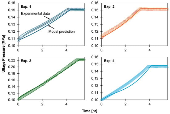
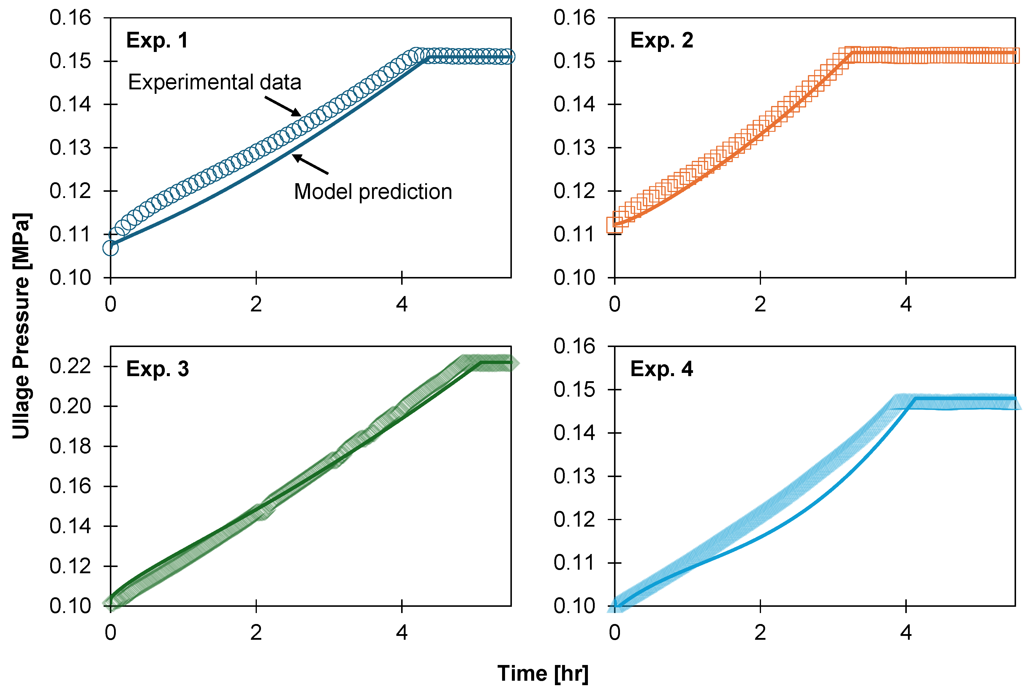
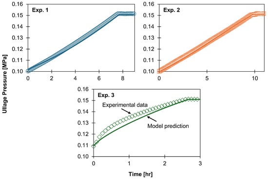
Figure 6 shows observed and predicted trends in ullage pressure during the first five hours of each experiment. For all experiments, the model predicted total pressurisation time to within a 10% deviation. However, the model did not accurately capture all transient pressure behaviour observed during this stage. This is a function of heat ingress, which occurs by both heat leak though the tank structure and heat transfer between the fluid and ambient environment. An overall HTC derived from the average heat ingress rate will capture the average rate of heat leak over time, but the variable ambient temperature will not capture transient heat leaks. Thus, defining ambient heating using a constant overall HTC and variable ambient temperature will predict an ullage pressure curve similar in shape to the ambient temperature curve.
Figure 6.
Ullage pressure during the pressurisation stage for the LN2 boil-off experiments. Symbols correspond to experimental data, and curves are model predictions.
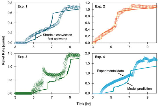
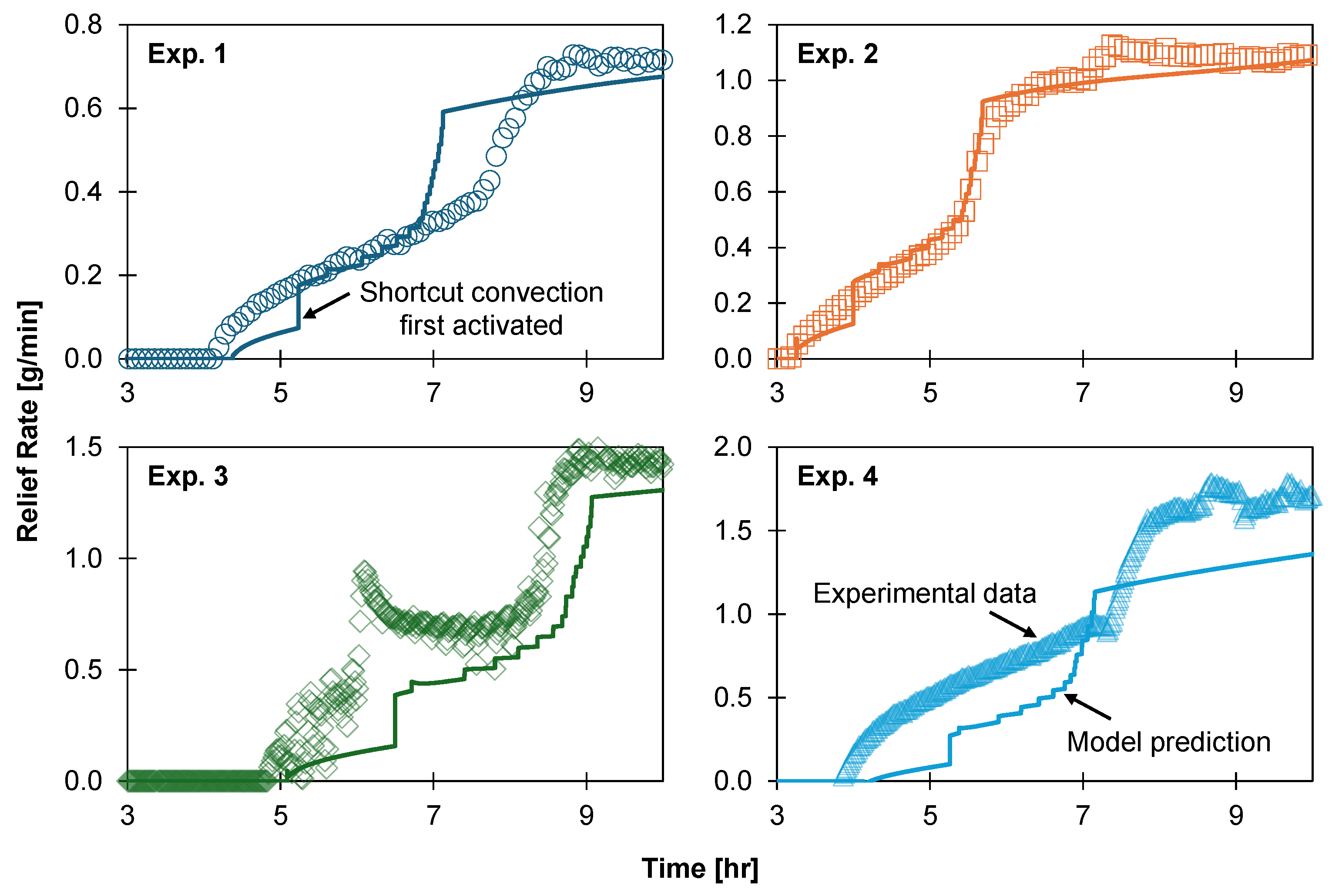
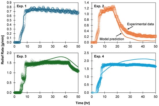
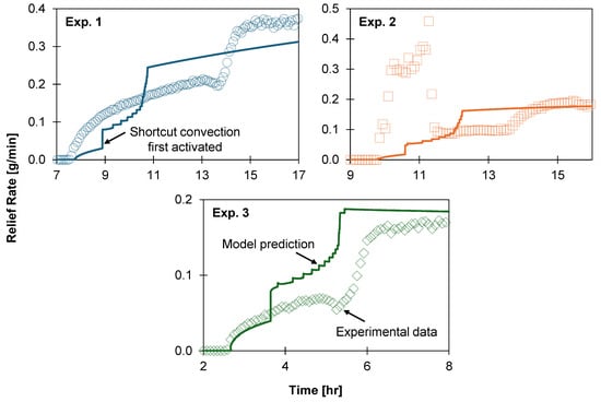
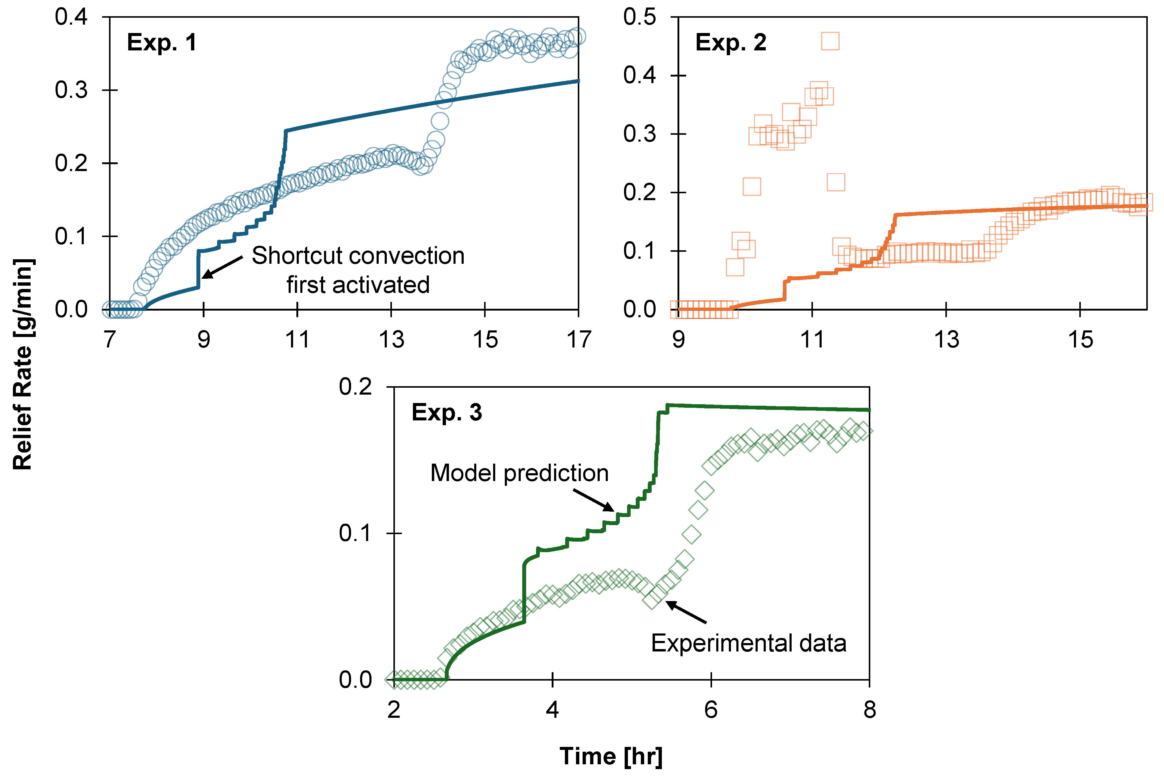
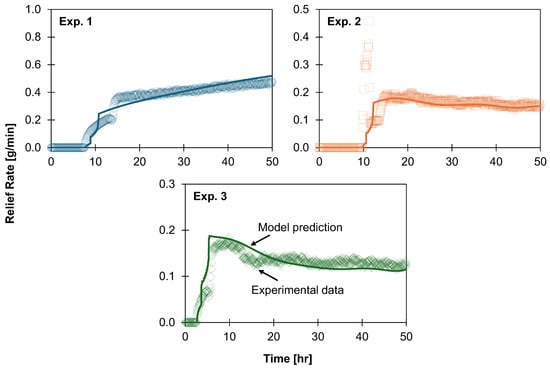
Figure 7 gives observed and predicted relief rates during the transient stage, and Figure 8 gives rates during the entire relief stage, for each experiment. The transient stage occurred in two parts, characterised by a more gradual increase in relief rate during the first than the second. The model captured this trend; however, its performance over the entire relief stage varied: it made excellent predictions of the steady-state relief rate for Exp. 1 and during the first 20 h of Exp. 2 but underestimated the relief rate thereafter, overestimated it for Exp. 3 after 20 h, and did both for Exp. 4. As with the deviation from observed ullage pressures, this is a consequence of defining ambient heating using a constant HTC and variable ambient temperature without capturing changes in heat leak through the tank structure during an experiment.
Figure 7.
Relief rates during the transient relief stage for the LN2 boil-off experiments. Symbols correspond to experimental data, and curves are model predictions.
Figure 8.
Relief rates for the LN2 boil-off experiments. Symbols correspond to experimental data, and curves are model predictions.
Of note in Figure 7 is the step change in relief rate predicted to occur shortly after the commencement of the relief stage (indicated in the figure for Exp. 1). This coincided with the activation of shortcut convection for the lowermost liquid layer, whereby heat ingress through the tank floor—significantly higher than that through each layer wall—was transferred directly to the film. The model predicted smaller step changes when activating shortcut convection for other layers. While such step changes are unphysical, they are an inherent consequence of dividing the liquid phase into a set of discrete layers: using smaller layers would yield a smoother transient relief curve.
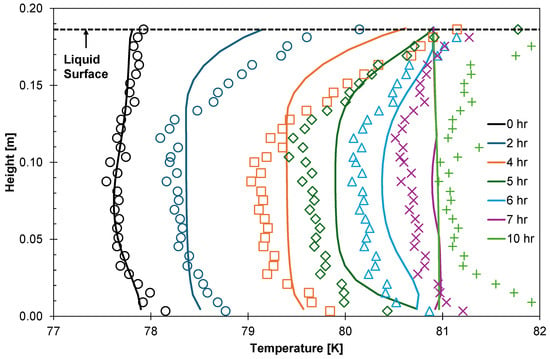
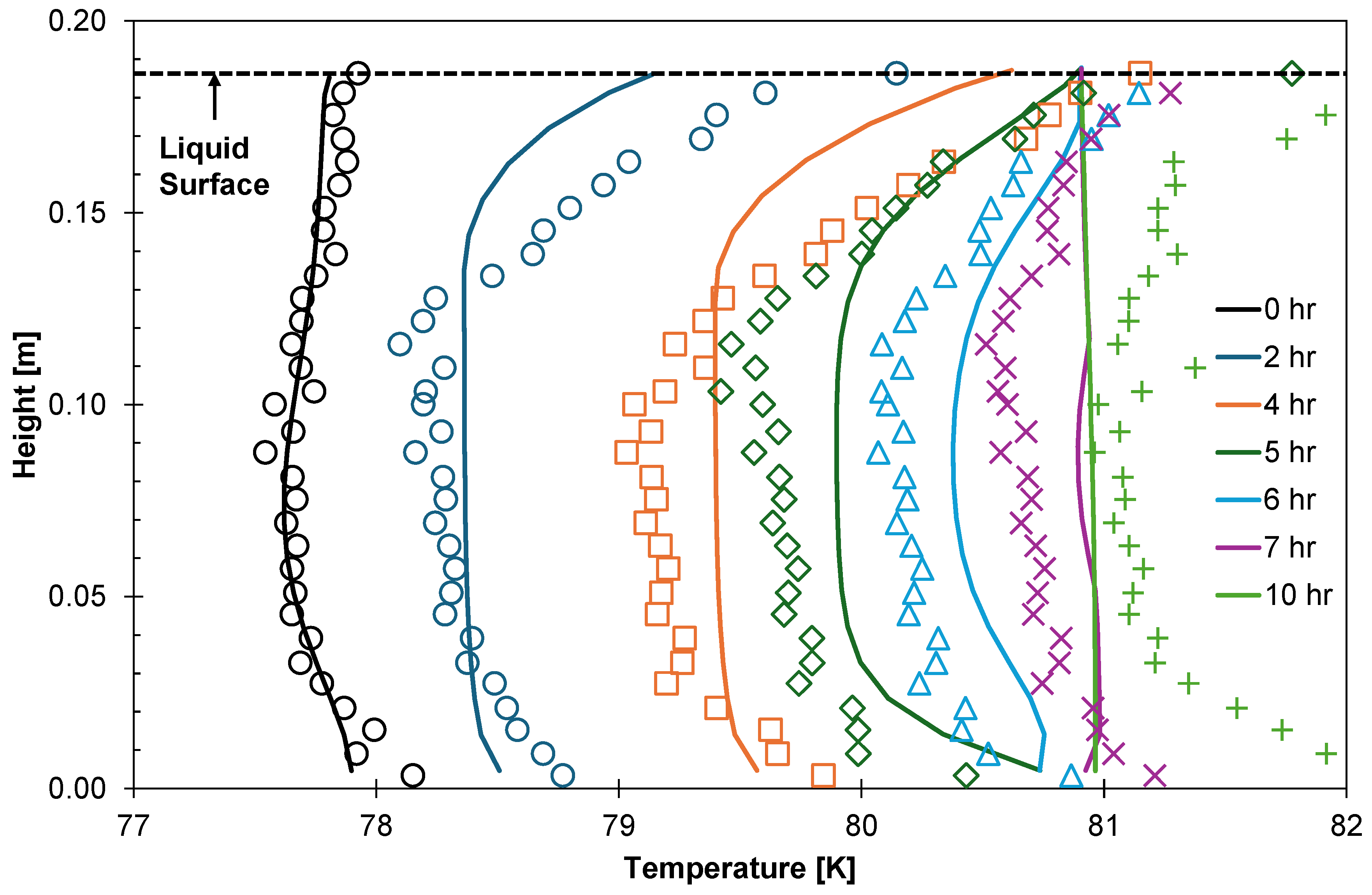
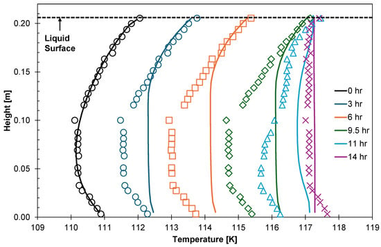
Figure 9 shows observed and predicted liquid temperatures during the first ten hours of Exp. 1. The model correctly predicted both the development of temperature gradients as the tank pressurised and the homogenisation of liquid temperature during the relief stage, albeit the latter occurred too quickly in the simulation. This may be in part a consequence of underpredicting the duration of the transient relief stage. Predicted temperatures tended to deviate from measured values by less than the 0.5 K uncertainty of the RTD sensors, apart from temperatures near the liquid surface and tank floor, which the model could underpredict by up to 1 K. However, temperatures measured in these areas may not be highly accurate: the superheated vapour and heat leak through the apparatus will warm the RTDs beneath the vapour–liquid interface and above the tank floor, causing these sensors to experience a higher temperature than that of the liquid. Figure 9 shows evidence of this: despite the model fixing the liquid surface to the saturated temperature, measured temperatures nearby exceed this by up to 1 K; similarly, measured temperatures near the tank floor exceed the temperature of saturated LN2 at 0, 7, and 10 hr. An alternative explanation for this phenomenon is the liquid superheating reported by Scurlock [26], in which case up to 1 K of superheating was observed during the relief stage.
Figure 9.
Liquid-phase temperature gradients for the first ten hours of LN2 Experiment 1; the relief stage began at four hours. Symbols correspond to experimental data, and curves are model predictions.
Table 3 summarises the performance of the model when simulating the LN2 experiments. Predicted pressurisation times fell within 7% of the observed value, and ullage pressure during pressurisation was reproduced with a root-mean-square deviation (RMSD) no greater than 5 kPa. Agreement was poorest for the duration of the transient relief stage, which was underpredicted by up to 38%, reflecting the layer-wise activation of shortcut convection and the resulting step changes in relief rate. On average, the model required five hours to simulate fifty hours of each experiment when using a constant step length of two seconds: this was strongly influenced by the choice of EOS model.
Table 3.
Summary of model performance when simulating LN2 experiments.
5.2. LNG Boil-Off
Al Ghafri et al. [14] reported three LNG boil-off experiments, presenting their pressurisation and relief rates, alongside temperature data for Exp. 2. Table 4 outlines the model inputs used to simulate the experiments.
Table 4.
Model inputs used to simulate the LNG boil-off experiments.
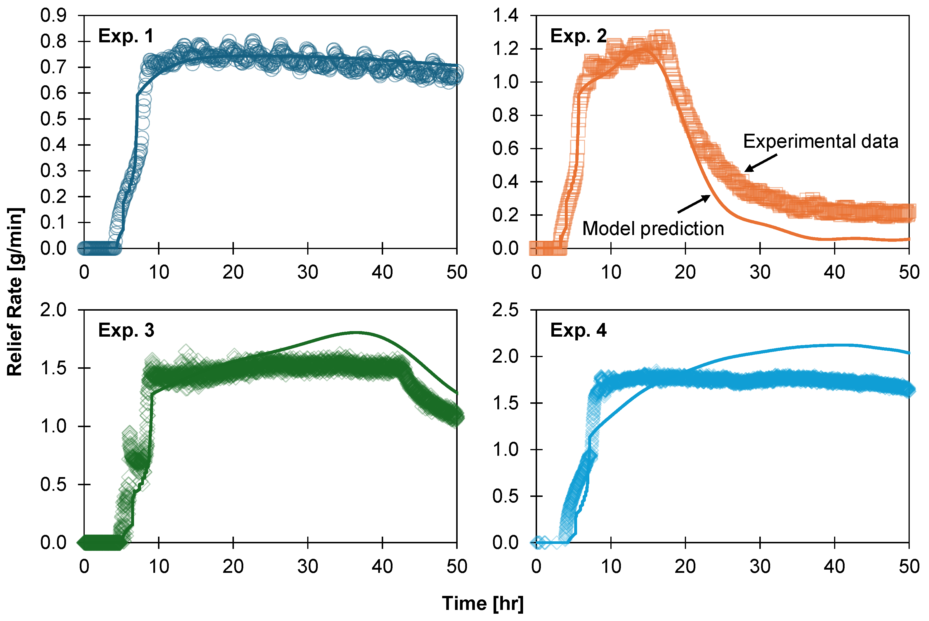
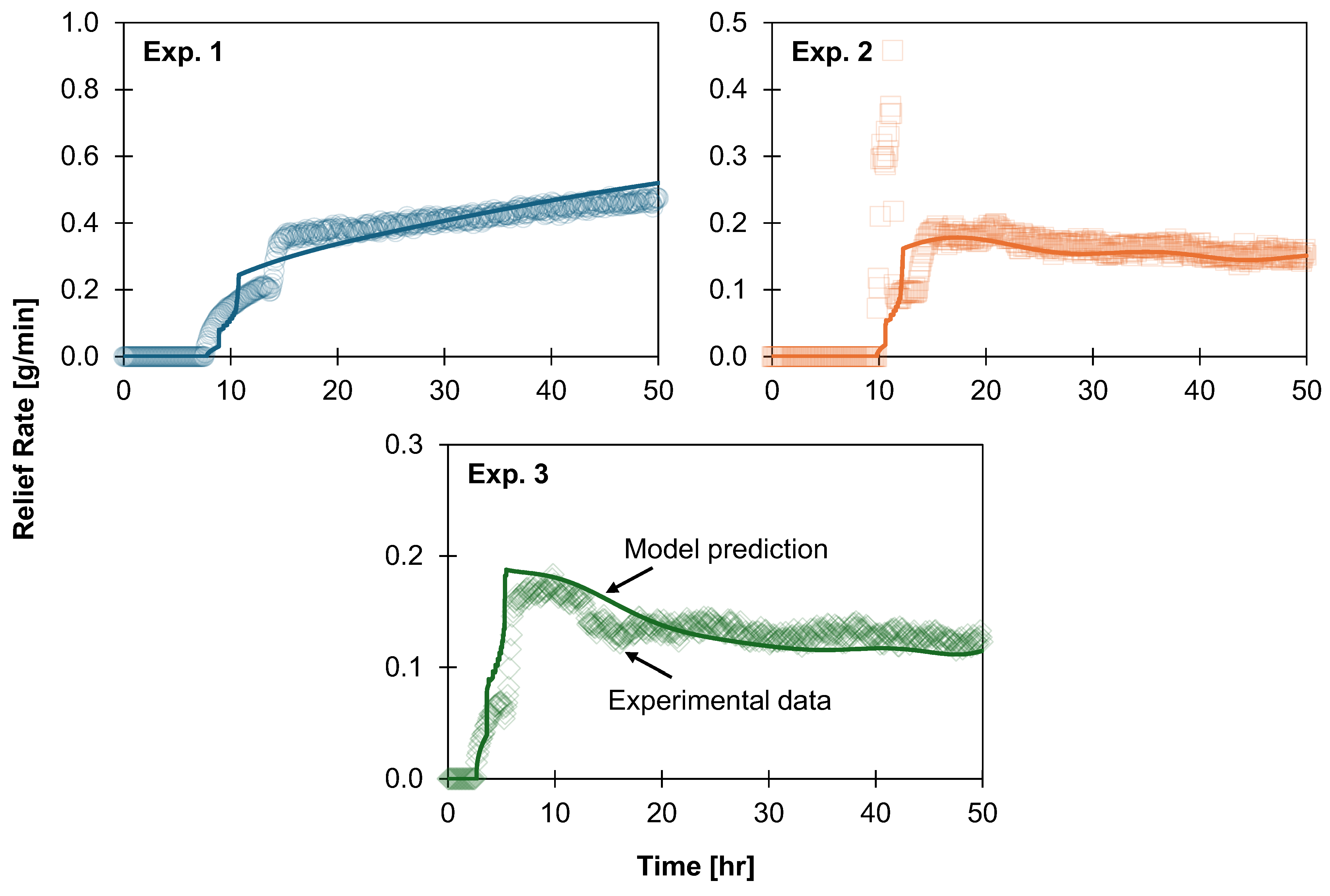
When simulating LNG boil-off, the model exhibited similar performance to the LN2 boil-off simulations. Per Figure 10, it accurately predicted pressurisation time despite not always capturing transient ullage pressure behaviour caused by variations in the experimental boundary temperature. The predicted duration of the transient relief stage for the LNG experiments (Figure 11) had a root-mean-square deviation of 2.3 h (or 44%), compared to 1 h (or 25%) for the LN2 experiments. However, the relief rate predictions (Figure 12) were improved relative to the LN2 experiments.
Figure 10.
Ullage pressure during the pressurisation stage for the LNG boil-off experiments. Symbols correspond to experimental data, and curves are model predictions.
Figure 11.
Relief rates during the transient relief stage for the LNG boil-off experiments. Symbols correspond to experimental data, and curves are model predictions.
Figure 12.
Relief rates for the LNG boil-off experiments. Symbols correspond to experimental data, and curves are model predictions.
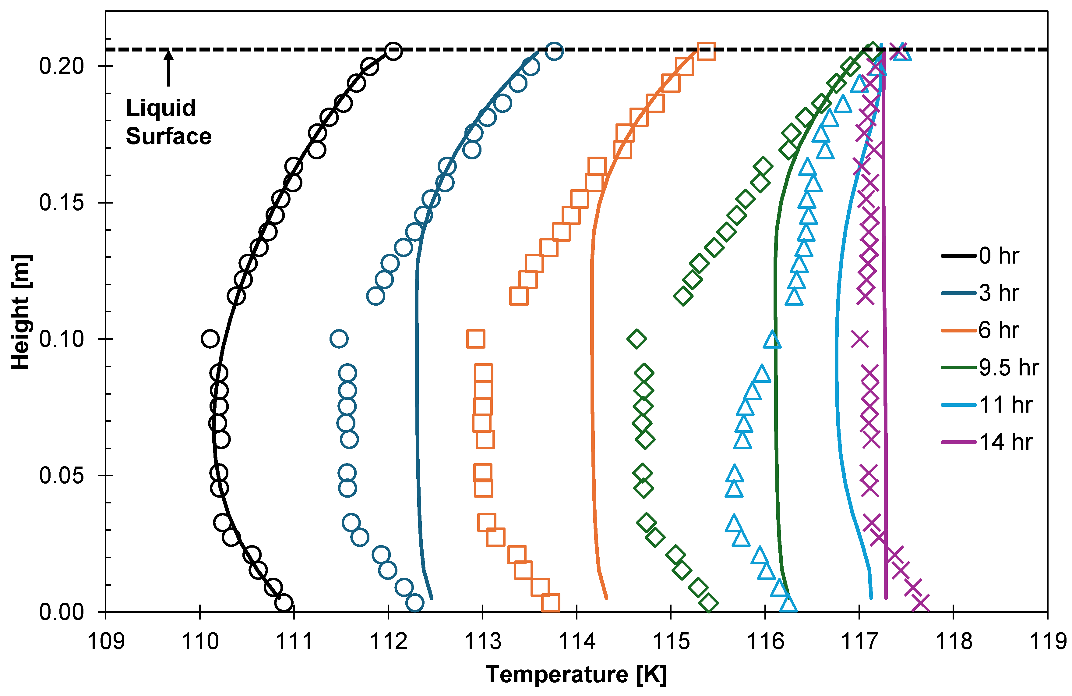
Predicted liquid temperature gradients for LNG (Figure 13) behaved similarly to those for LN2 in Figure 9, including the accelerated prediction of homogenisation after the tank pressurised. The LNG experiments occurred in the same apparatus as the LN2 experiments, and the model used the same method to calculate ambient heating; thus, the issues discussed earlier also affected the LNG boil-off simulations. During the relief stage, temperatures measured during the LNG experiment (14 h, Figure 13) were more homogeneous than for the LN2 experiment (10 h, Figure 9): temperatures recorded near the top and bottom of the LN2 were up to 1 K higher than in the middle. During the LN2 experiment, the vapour was more superheated relative to the liquid, and total heat ingress into the apparatus was higher; combined, these effects warmed the RTDs near the top and bottom of the liquid to a greater extent. As with the LN2 experiment, the liquid below the surface may be superheated [26], with up to 1 K of superheating observed during the relief stage.
Figure 13.
Liquid-phase temperature gradients for the first fourteen hours of LNG Experiment 2; the relief stage began at 9.5 h. Symbols correspond to experimental data, and curves are model predictions.
Table 5 summarises the performance of the model when simulating the LNG experiments. Predicted pressurisation times fell within 3% of the observed value, and ullage pressure during pressurisation was reproduced with a root-mean-square deviation (RMSD) no greater than 4 kPa. Agreement was poorest for the duration of the transient relief stage, which was underpredicted by up to 55%, reflecting the layer-wise activation of shortcut convection and the resulting step changes in relief rate. On average, the model required nine hours to simulate fifty hours of each experiment when using a constant step length of two seconds: this was strongly influenced by the choice of EOS model.
Table 5.
Summary of model performance when simulating LNG experiments.
5.3. Discussion
Alongside the uncertainty in measured temperatures and the potential for superheating of the liquid during the relief stage, the following aspects of the model contribute to the deviation of its predictions from experimental results:
- The empirical correlations used to predict convective heat transfer and boundary layer flowrate.
- Assuming steady-state heat conduction through the tank walls.
- Ignoring radiative heat transfer in the ullage.
- The one-dimensional discretisation of the fluid and the assumption of homogeneous properties within each layer.
- The equal volume remeshing procedure.
The model uses empirical correlations to calculate vapour–film heat transfer and resolve the convection boundary layer within the liquid. While this work does not introduce new adjustable parameters, the correlations include empirical coefficients used to fit experimental data.
The model calculated the vapour–film heat transfer coefficient using the McAdams correlation for convection above a cooled, horizontal surface [25]:
where is the average Nusselt number, and C1 is a coefficient equal to 0.27; the magnitude of C1 will affect vapour–film heat transfer, with higher values increasing the rate thereof. Its value will affect predictions of pressurisation time and steady-state relief rate.
The model calculated the flowrate of the convective boundary layer using a series of correlations for the average layer velocity and thickness depending on the flow type. Having found the boundary layer thickness and flow velocity, a modified form of the Schallhorn et al. [33] equation gives the molar flowrate in the boundary layer:
where C2 is a coefficient equal to 0.0833 for a laminar boundary layer and 0.1436 for a turbulent boundary layer; the model selects the appropriate value assuming the laminar–turbulent transition occurs at a Rayleigh number of 1 × 10⁹. The magnitude of C2 will affect the boundary layer flowrate, with higher values yielding faster molar flows. This will affect the predictions of temperature stratification in the liquid; for example, the model predicted a smaller-than-observed conduction domain thickness for the LN2 (Figure 9) and LNG (Figure 13) experiments, suggesting that the value of this coefficient could be reduced.
Finally, all correlations used by the model when predicting convective flow and heat transfer assume a steady state. However, the systems simulated by the model exhibited transient behaviour, particularly as the conduction domain developed below the interface during pressurisation and at the start of the relief stage. The use of steady-state correlations to simulate transient behaviour introduces uncertainty.
The model assumes steady-state heat conduction through the tank that is, all ambient heat ingress enters the fluid, with none heating the tank structure. By failing to account for this heat accumulation, the model can overpredict the pressurisation and relief rates: ambient heat which would have otherwise increased the temperature of the tank structure boils the liquid.
In the experiments simulated here, the effect of assuming steady-state conduction through the tank is negligible. Based on BOG cell specifications presented by Perez et al. [13], tank thermal masses were 0.06% of the LN2 and LNG thermal mass, given a 90% fill.
However, for well-insulated systems, heat accumulation could be significant. The heat capacity of perlite—commonly used to insulate large tanks—is over one hundred times greater than that of the stainless steel used to construct the BOG cell. Therefore, accurate simulation of well-insulated systems, such as industrial LNG storage tanks, will require any model to consider transient heat conduction through the tank.
Heat transfer by radiation will occur within the ullage, with the hotter roof and walls radiating heat to the cooler fluid. This will heat the vapour–liquid interface; by ignoring this extra source of heat ingress to the film, the model may underpredict the boil-off and thus pressurisation and relief rates. Given the most conservative assumptions—that 100% of the radiation emitted by the roof and walls is incident on the vapour–liquid interface, and the vapour absorbs no radiation—radiative heating of the interface is up to 0.2% of convective heat transfer between the vapour and film.
The model treats the fluid in only one spatial dimension, assuming that each layer is of homogeneous pressure, temperature, and composition. Real storage systems exhibit radial variation which this treatment cannot represent. Within the convection domain, the model evaluates a circulation rate, but the enthalpy carried at this flow is evaluated at the average layer temperature rather than at the higher temperature of the near-wall fluid. Thus, the boundary layer is resolved for the purpose of calculating a flowrate but not as a thermally distinct region. Likewise, the convection cell is idealized as an upward stream along the wall and a downward plume in the tank centre, instead of the three-dimensional structure present in a real system.
These simplifications are of limited consequence for this study, as pressurisation and relief rates are most influenced by the vertical temperature profile, which the model resolves. They do, however, prevent the prediction of locally varying behaviour, such as that arising from non-uniform insulation performance or asymmetric heating through a tank’s internal structure.
Layers of a given phase are constrained to equal volume, with a remeshing procedure redistributing the fluid between adjacent layers should their volumes diverge during a step. This procedure conserves the total enthalpy of the phase and the amount of each species within it. However, it is not free of numerical diffusion: each redistribution mixes the fluid across a layer boundary, smoothing the temperature profile. Should this effect become substantial, the model may underpredict the sharpness of the thermal gradient beneath the film and may predict homogenisation of the liquid more rapidly than observed. This effect is difficult to separate from that of the boundary layer flowrate coefficient discussed above, as both will act on the predicted thickness of the conduction domain.
The applicability of shortcut convection beyond the conditions simulated here also warrants comment. Shortcut convection relies on the assumption that convective heat transfer within the liquid is rapid relative to ambient heating. In this work, the shortcut was only necessary during the isobaric (relief) stage, for the reasons given in Section 4.2.4. This approximation would be less appropriate under conditions in which the interface temperature changes faster than the bulk liquid can respond, such as rapid depressurisation. With respect to geometry, shortcut convection is most applicable where a substantial fraction of ambient heat enters through the tank floor and lower walls, as this drives circulation throughout the liquid. It is likely less applicable if heat ingress were concentrated near the top of the liquid or into the ullage, which promotes stable stratification. Similarly, tank aspect ratio is also material, with taller, slender vessels presenting a longer convective path that may not suit the assumption underpinning shortcut convection.
Finally, the model assumes a quiescent liquid with a flat, stationary vapour–liquid interface, with no accounting for tank motion. In maritime transport, sloshing mechanically mixes the liquid, disrupting the stratification resolved by the model, while increasing the area of the vapour–liquid interface. Both effects will impact boil-off production; thus, the predictions presented here are applicable to conditions under which motion-induced mixing is small relative to convection, such as static storage.
6. Conclusions and Future Work
This work introduced a new, predictive model capable of simulating boil-off from a variety of fluids under a range of storage conditions. It accounts for thermal and compositional gradients in the liquid with layers coupled by heat and mass transfer equations. During pressurisation, the model divides the liquid into conduction and convection domains and calculates boundary layer and recirculation flowrates within the latter. During isobaric operation (relief), the model applies a shortcut convection term to transfer ambient heat ingress from a layer to the surface of the liquid, where it generates boil-off instead of heating the liquid. This term reproduces the boil-off rate without resolving the superheating which drives boil-off in a real system, and this approach is expected to hold wherever convective transport is rapid relative to ambient heating. Unlike previously published works, this model does not require manipulation of adjustable parameters to fit the boil-off rate, heat transfer rates, or the conduction domain thickness to experimental data.
A set of validation cases demonstrated the accuracy of the model. The model predicted pressurisation time to within 10% of observed values for LN2 and to within 5% for LNG and captured both the transient relief stage and the evolution of liquid temperature gradients during and after pressurisation. The model’s predictions are within the uncertainty arising from available specifications of the experimental boundary conditions. The model introduced in this work offers a range of benefits to the existing LNG and future CO2 and even LH2 supply chains.
Several avenues remain for the further development and validation of the model. The most immediate is validation against industrial-scale data, for which the model may first need to be extended to describe transient heat conduction through the tank wall and insulation. Extension to LH2 will require tracking of the ortho- and para-isomer fractions as compositional variables, with the enthalpy of conversion being included as a source term in the layer energy balances. Finally, extension to carbon dioxide will require further validation at the high pressures and near-critical conditions under which it is stored.
Author Contributions
Conceptualization, E.F.M.; methodology, V.J. and E.F.M.; software, V.J.; investigation, V.J.; writing—original draft, V.J.; writing—review and editing, S.A.G. and E.F.M.; supervision, S.A.G. and E.F.M.; funding acquisition, E.F.M. All authors have read and agreed to the published version of the manuscript.
Funding
This work was funded by the Future Energy Exports CRC (www.fenex.org.au), whose activities are funded by the Australian Government’s Cooperative Research Centre Program. This is FEnEx CRC document number 2026/21.RP1.0076-FNX-MILE0999.
Data Availability Statement
The original contributions presented in this study are included in the article. Further inquiries can be directed to the corresponding author.
Acknowledgments
We acknowledge Peter Falloon and Darren Rowland for their work on the ThermoFAST software package used in this work.
Conflicts of Interest
The authors declare no conflicts of interest.
Nomenclature
The following abbreviations are used in this manuscript:
| amb. | Ambient |
| BOG | Boil-off Gas |
| CCUS | Carbon Capture, Utilisation, and Storage |
| CO2 | Carbon Dioxide |
| EOS | Equation of State |
| Eqn. | Equation |
| Exp. | Experiment |
| FL | Film–Liquid |
| GERG | Groupe Européen de Recherches Gazières (European Gas Research Group) |
| H2 | Hydrogen |
| HTC | Heat Transfer Coefficient |
| L | Liquid, used in sub- or superscript to denote phase property |
| LH2 | Liquid Hydrogen |
| LN2 | Liquid Nitrogen |
| LNG | Liquefied Natural Gas |
| MTC | Mass Transfer Coefficient |
| ODE | Ordinary Differential Equation |
| PC | Personal Computer |
| RMSD | Root-Mean-Square Deviation |
| RTD | Resistance Temperature Detector |
| sat. | Saturated |
| SC | Shortcut Convection |
| SHV | Superheated Vapour |
| V | Vapour, used in sub- or superscript to denote phase property |
| VF | Vapour-Film |
| The following symbols are used in this manuscript: | |
| A | Area, m2 |
| Dij | Diffusion coefficient of species i in solvent j, m2/s |
| Gr | Grashof number |
| h | Specific enthalpy, J/mol |
| Average heat transfer coefficient, W/m2/K | |
| Specific enthalpy of the liquid film, J/mol | |
| Specific enthalpy of the boil-off gas, J/mol | |
| H | Total enthalpy, J |
| kB | Boltzmann constant, 1.380649E-23 J/K |
| n | Number of moles, mol |
| Average Nusselt number | |
| p | Pressure, MPa |
| Pr | Prandtl number |
| q | Heat transfer rate, W |
| Ra | Rayleigh number |
| Rs | Stability ratio |
| t | Time, s |
| T | Temperature, K |
| u | Velocity, m/s |
| UFL | Film–liquid heat transfer coefficient, W/m2/K |
| ULL | Liquid–liquid heat transfer coefficient, W/m2/K |
| UVF | Vapour–film heat transfer coefficient, W/m2/K |
| V | Volume, m3 |
| x | Distance, m |
| xi | Mole fraction of species i |
| β | Coefficient of thermal expansion, 1/K |
| δ | Thickness, m |
| ΔT | Temperature difference, K |
| η | Dynamic viscosity, Pa∙s |
| λ | Thermal conductivity, W/m/K |
| ν | Kinematic viscosity, m2/s |
| ρ | Mass density, kg/m3 |
| σ | Lennard–Jones collision diameter, m |
References
- Energy Information Administration. International Energy Outlook 2023; Department of Energy: Washington, DC, USA, 2023.
- International Energy Agency. Energy Technology Perspectives 2020 Special Report on Carbon Capture Utilisation and Storage; IEA: Paris, France, 2020.
- International Energy Agency. World Energy Outlook 2023; IEA: Paris, France, 2023.
- Lemmon, E.W.; Bell, I.H.; Huber, M.L.; McLinden, M.O. NIST Standard Reference Database 23: Reference Fluid Thermodynamic and Transport Properties-REFPROP; Version 10.0; National Institute of Standards and Technology: Gaithersburg, MD, USA, 2018.
- Setzmann, U.; Wagner, W. A New Equation of State and Tables of Thermodynamic Properties for Methane Covering the Range from the Melting Line to 625 K at Pressures up to 100 MPa. J. Phys. Chem. Ref. Data 1991, 20, 1061–1155. [Google Scholar] [CrossRef] [Scilit]
- Leachman, J.W.; Jacobsen, R.T.; Penoncello, S.G.; Lemmon, E.W. Fundamental Equations of State for Parahydrogen, Normal Hydrogen, and Orthohydrogen. J. Phys. Chem. Ref. Data 2009, 38, 721–748. [Google Scholar] [CrossRef] [Scilit]
- Span, R.; Wagner, W. A New Equation of State for Carbon Dioxide Covering the Fluid Region from the Triple-Point Temperature to 1100 K at Pressures up to 800 MPa. J. Phys. Chem. Ref. Data 1996, 25, 1509–1596. [Google Scholar] [CrossRef] [Scilit]
- Hasan, M.M.F.; Zheng, A.M.; Karimi, I.A. Minimizing Boil-off Losses in Liquefied Natural Gas Transportation. Ind. Eng. Chem. Res. 2009, 48, 9571–9580. [Google Scholar] [CrossRef] [Scilit]
- Dimopoulos, G.; Frangopoulos, C. A Dynamic Model for Liquefied Natural Gas Evaporation During Marine Transportation. Int. J. Thermodyn. 2008, 11, 123–131. [Google Scholar]
- Miana, M.; del Hoyo, R.; Rodrigálvarez, V.; Valdés, J.R.; Llorens, R. Calculation models for prediction of Liquefied Natural Gas (LNG) ageing during ship transportation. Appl. Energy 2010, 87, 1687–1700. [Google Scholar] [CrossRef] [Scilit]
- Pellegrini, L.A.; Moioli, S.; Brignoli, F.; Bellini, C. LNG Technology: The Weathering in Above-Ground Storage Tanks. Ind. Eng. Chem. Res. 2014, 53, 3931–3937. [Google Scholar] [CrossRef] [Scilit]
- Migliore, C.; Salehi, A.; Vesovic, V. A non-equilibrium approach to modelling the weathering of stored Liquefied Natural Gas (LNG). Energy 2017, 124, 684–692. [Google Scholar] [CrossRef] [Scilit]
- Perez, F.; Al Ghafri, S.Z.S.; Gallagher, L.; Siahvashi, A.; Ryu, Y.; Kim, S.; Kim, S.G.; Johns, M.L.; May, E.F. Measurements of boil-off gas and stratification in cryogenic liquid nitrogen with implications for the storage and transport of liquefied natural gas. Energy 2021, 222, 119853. [Google Scholar] [CrossRef] [Scilit]
- Al Ghafri, S.Z.S.; Perez, F.; Park, K.H.; Gallagher, L.; Warr, L.; Stroda, A.; Siahvashi, A.; Ryu, Y.; Kim, S.; Kim, S.G.; et al. Advanced boil-off gas studies for liquefied natural gas. Appl. Therm. Eng. 2021, 189, 116735. [Google Scholar] [CrossRef] [Scilit]
- Huerta, F.; Vesovic, V. A realistic vapour phase heat transfer model for the weathering of LNG stored in large tanks. Energy 2019, 174, 280–291. [Google Scholar] [CrossRef] [Scilit]
- Jung, B.; Park, K.; Sohn, Y.; Oh, J.; Lee, J.C.; Jung, H.W.; Seo, Y.; Lim, Y. Prediction model of LNG weathering using net mass and heat transfer. Energy 2022, 247, 123325. [Google Scholar] [CrossRef] [Scilit]
- Al Ghafri, S.Z.S.; Swanger, A.; Park, K.H.; Jusko, V.; Ryu, Y.; Kim, S.; Kim, S.G.; Zhang, D.; Seo, Y.; Johns, M.L.; et al. Advanced boil-off gas studies of liquefied natural gas used for the space and energy industries. Acta Astronaut. 2022, 190, 444–454. [Google Scholar] [CrossRef] [Scilit]
- Kunz, O.; Wagner, W. The GERG-2008 Wide-Range Equation of State for Natural Gases and Other Mixtures: An Expansion of GERG-2004. J. Chem. Eng. Data 2012, 57, 3032–3091. [Google Scholar] [CrossRef] [Scilit]
- Daigle, M.J.; Smelyanskiy, V.N.; Boschee, J.; Foygel, M. Temperature Stratification in a Cryogenic Fuel Tank. J. Thermophys. Heat Transf. 2012, 27, 116–126. [Google Scholar] [CrossRef] [Scilit]
- Wang, Z.; Sharafian, A.; Mérida, W. Thermal stratification and rollover phenomena in liquefied natural gas tanks. Energy 2022, 238, 121994. [Google Scholar] [CrossRef] [Scilit]
- Kim, S.; Lee, J.-G.; Kim, S.; Heo, J.; Bang, C.S.; Lee, D.-K.; Lee, H.; Park, G.; Lee, D.; Lim, Y. Experiment and simulation of LNG self-pressurization considering temperature distribution under varying liquid level. Energy 2024, 290, 130071. [Google Scholar] [CrossRef] [Scilit]
- Chin, J.H.; Harper, E.Y.; Hines, F.L.; Hurd, S.E.; Vliet, G.C. Analytical and Experimental Study of Stratification and Liquid-Ullage Coupling; NASA-CR-80472; George C. Marshall Space Flight Centre, National Aeronautics and Space Administration: Huntsville, AL, USA, 1965. [Google Scholar]
- Chapman, S.J. Fortran for Scientists and Engineers, 4th ed.; McGraw-Hill Education: New York, NY, USA, 2018. [Google Scholar]
- Jusko, V. BoilFAST: Cryogenic Boil-off Simulator; Version 2; Fluid Sciences and Resources Group, The University of Western Australia: Perth, Australia, 2025. [Google Scholar]
- McAdams, W.H. Heat Transmission, 3rd ed.; McGraw-Hill: New York, NY, USA, 1954. [Google Scholar]
- Scurlock, R.G. Stratification, Rollover and Handling of LNG, LPG and Other Cryogenic Liquid Mixtures; Springer International Publishing: Cham, Switzerland, 2016. [Google Scholar]
- Globe, S.; Dropkin, D. Natural-Convection Heat Transfer in Liquids Confined by Two Horizontal Plates and Heated from Below. J. Heat Transf. 1959, 81, 24–28. [Google Scholar] [CrossRef] [Scilit]
- Arjomandnia, P.; Tade, M.O.; Pareek, V.; May, E.F. Analysis of available data from liquefied natural gas rollover incidents to determine critical stability ratios. AIChE J. 2014, 60, 362–374. [Google Scholar] [CrossRef] [Scilit]
- Pickering, G. Prediction of Rollover for Stratified Liquefied Natural Gas in Storage Tanks. Master’s Thesis, School of Mechanical and Chemical Engineering, The University of Western Australia, Perth, Australia, 2017. [Google Scholar]
- Kakac, S.; Yener, Y.; Pramuanjaroenkij, A. Convective Heat Transfer, 3rd ed.; CRC Press: Boca Raton, FL, USA, 2014. [Google Scholar]
- Eckert, E.R.G.; Jackson, T.W. Analysis of Turbulent Free-Convection Boundary Layer on Flat Plate; NACA-TN-2207; Lewis Flight Propulsion Laboratory, National Advisory Committee for Aeronautics: Cleveland, OH, USA, 1950.
- Raithby, G.D.; Hollands, K.G.T. Natural Convection. In Handbook of Heat Transfer, 3rd ed.; Rohsenow, W.M., Hartnett, J.P., Cho, Y.I., Eds.; McGraw-Hill: New York, NY, USA, 1998; pp. 4.10–4.14. [Google Scholar]
- Schallhorn, P.; Campbell, D.; Chase, S.; Piquero, J.; Fortenberry, C.; Xiaoyi, L.; Grob, L. Upper Stage Tank Thermodynamic Modeling Using SINDA/FLUINT. In Proceedings of the 42nd AIAA/ASME/SAE/ASEE Joint Propulsion Conference, Sacramento, CA, USA, 9–12 July 2006. [Google Scholar]
- Tellep, D.M.; Harper, E.Y. Approximate Analysis of Propellant Stratification. AIAA J. 1963, 1, 1954–1956. [Google Scholar] [CrossRef] [Scilit] [PubMed]
- Falloon, P.E.; Rowland, D.; Baker, C.J.; May, E.F. ThermoFAST: Thermodynamic Calculator for Fluid Mixture Properties; Version 2.2.1; Fluid Sciences and Resources Group, The University of Western Australia: Perth, Australia, 2025. [Google Scholar]
- Span, R.; Lemmon, E.W.; Jacobsen, R.T.; Wagner, W.; Yokozeki, A. A Reference Equation of State for the Thermodynamic Properties of Nitrogen for Temperatures from 63.151 to 1000 K and Pressures to 2200 MPa. J. Phys. Chem. Ref. Data 2000, 29, 1361–1433. [Google Scholar] [CrossRef] [Scilit]
- Peng, D.-Y.; Robinson, D.B. A New Two-Constant Equation of State. Ind. Eng. Chem. Fundam. 1976, 15, 59–64. [Google Scholar] [CrossRef] [Scilit]
- Lemmon, E.W.; Jacobsen, R.T. Viscosity and Thermal Conductivity Equations for Nitrogen, Oxygen, Argon, and Air. Int. J. Thermophys. 2004, 25, 21–69. [Google Scholar] [CrossRef] [Scilit]
- Bell, I.H. Probing the link between residual entropy and viscosity of molecular fluids and model potentials. Proc. Natl. Acad. Sci. USA 2019, 116, 4070–4079. [Google Scholar] [CrossRef] [Scilit] [PubMed]
- Perez, F. LNG Thermodynamic Data for Key Engineering Challenges. Ph.D. Thesis, The University of Western Australia, Perth, Australia, 2020. [Google Scholar]
- Barriero-Villaverde, D.; Cantiani, A.; Mendez, M.A. On the complex interplay of temperature, phase change and natural convection in self-pressurization—An investigation using segregated modeling. Int. J. Heat Mass Transf. 2026, 269, 129150. [Google Scholar] [CrossRef] [Scilit]
- Jusko, V. Understanding and Predicting Boil-off from Cryogenic Liquids. Ph.D. Thesis, The University of Western Australia, Perth, Australia, 2024. [Google Scholar]

Disclaimer/Publisher’s Note: The statements, opinions and data contained in all publications are solely those of the individual author(s) and contributor(s) and not of MDPI and/or the editor(s). MDPI and/or the editor(s) disclaim responsibility for any injury to people or property resulting from any ideas, methods, instructions or products referred to in the content. |
© 2026 by the authors. Licensee MDPI, Basel, Switzerland. This article is an open access article distributed under the terms and conditions of the Creative Commons Attribution (CC BY) license.