


Abstract
The increasing integration of photovoltaic systems into modern power grids requires forecasting models that not only provide accurate predictions but also reliable uncertainty quantification under evolving operating conditions. In this paper, we propose an Out-of-distribution-aware time series conformal prediction framework with adaptive retraining, designed to address key limitations of standard conformal prediction methods in temporally dependent and dynamically changing environments. The framework is built upon the Ensemble batch prediction intervals method, which enables distribution-free uncertainty quantification without relying on a fixed calibration set, making it particularly suitable for time series applications. To ensure robustness to distribution shifts, a conformal out-of-distribution detection module is incorporated, where out-of-distribution detection is formulated as a hypothesis testing problem and enhanced through calibration-conditional p-values obtained via the Simes correction, providing conservative false-positive control intended to limit unnecessary model retraining. The proposed framework demonstrates superior performance compared to state-of-the-art approaches in uncertainty quantification, while conformal out-of-distribution detection reduces false positives and the adaptive retraining mechanism ensures effective adaptation to evolving data distributions in real-world scenarios.
1. Introduction
The rapid integration of renewable energy sources into modern power systems introduces both opportunities and challenges for grid operators. Among renewables, solar photovoltaic (PV) energy has witnessed the fastest growth in installed capacity worldwide. According to the International Energy Agency, global PV capacity is expected to exceed 4000 GW by 2030, highlighting its central role in the ongoing energy transition [1]. However, the inherently intermittent and weather-dependent nature of solar generation presents substantial forecasting challenges [2,3], particularly when forecasts must be translated into uncertainty-aware decision support for operators [4].
Traditional time series forecasting methods, including statistical approaches and machine learning models, typically aim to minimize point prediction errors [5,6,7]. To ensure reliable integration of PV into modern grids, forecasting models must not only provide accurate point predictions but also quantify uncertainty. While deterministic point forecasts are informative, probabilistic forecasts and calibrated prediction intervals are essential for energy trading, reserve scheduling, and risk management [8]. However, point forecasts alone cannot adequately capture the inherent uncertainty of solar generation. This uncertainty becomes critical in operational decision-making processes, where system operators and energy traders require not only predictions but also reliable measures of confidence.
Conformal prediction (CP) has recently emerged as a powerful framework for uncertainty quantification in machine learning, offering valid prediction intervals with user-specified coverage guarantees under the assumption of data exchangeability (Data exchangeability refers to the assumption that the joint probability distribution of a dataset remains unchanged under any permutation of the data samples. This property is less restrictive than the assumption of independent and identically distributed (i.i.d.) data, as it allows for certain dependencies among samples, provided that their joint distribution is symmetric) CP adjusts prediction intervals on the test set by analyzing the residuals obtained from a held-out portion of the training data, commonly referred to as the calibration set. The method ensures statistical validity by transforming point estimates into intervals that, with a predefined probability, capture the true observation [9]. Unlike many probabilistic approaches, CP is model-agnostic, computationally efficient, and provides rigorous finite-sample coverage guarantees. These properties make CP particularly appealing for renewable energy forecasting tasks.
Recent years have witnessed an increasing use of CP techniques for time series forecasting across diverse application areas [10,11]. Nevertheless, only a small number of studies have focused on applying CP to renewable energy forecasting problems, including solar and wind power generation [12,13,14]. In all of these works, standard CP algorithms are employed under the assumption of data exchangeability. However, data exchangeability represents a major challenge when applying standard CP algorithms, as time-series data generated by PV plants typically violate this assumption. To the best of our knowledge, no prior study has explored CP methods explicitly tailored for time series data that do not rely on the exchangeability assumption and are therefore better suited for non-stationary, real-world environments.
The second challenge with CP methods is sensitivity to distribution shifts. When changes in the data distribution occur, the reliability of conformal prediction intervals may decline. For example, under non-stationary meteorological conditions or during sudden operational changes in PV power plants, the coverage guarantees can deteriorate [15]. Addressing this challenge requires approaches that integrate Out-Of-Distribution (OOD) detection with conformal calibration, ensuring prediction intervals remain reliable when covariate shifts occur. Recent contributions in weighted conformal prediction [15], doubly robust calibration [16], and training-conditional coverage [17] emphasize the importance of adapting CP to real-world non-stationary environments. However, no prior work has investigated Conformal OOD (COOD) detection in the context of solar forecasting.
In this work, we propose an Out-of-Distribution-Aware Time Series Conformal Prediction framework with Adaptive Retraining (OOD-CPAR) that jointly addresses both challenges discussed above. To mitigate the first challenge related to the exchangeability assumption, OOD-CPAR builds upon the time-series conformal prediction framework based on the Ensemble Batch Prediction Intervals (ENBPI) method, which relaxes the strict requirement of data exchangeability that constrains conventional CP approaches. This enables the generation of valid prediction intervals for sequential, autocorrelated data produced by PV plants. Second, the framework introduces an adaptive component designed to maintain calibration under non-stationary and OOD conditions. It integrates COOD detection to continuously monitor incoming data streams and selectively retrains the predictive model when significant distribution shifts are identified. The false positive rate (FPR) is defined as the probability that the algorithm falsely signals a distribution shift when the underlying data distribution has not actually changed. By controlling FPR the framework maintains the desired sensitivity level. This control mechanism prevents unnecessary retraining events, ensuring that model updates occur only when distribution shifts are detected, thereby preserving both computational efficiency and consistent predictive reliability.
The main contributions of this paper are as follows:
- We propose OOD-CPAR, an integrated framework combining time-series conformal prediction, conformal OOD detection, and adaptive retraining for uncertainty-aware PV power forecasting under distribution shifts.
- We present the first application of a time series CP framework (ENBPI framework) to solar PV plant data, which relaxes the data exchangeability assumption that constrains conventional CP methods.
- We introduce the first COOD detection mechanism specifically designed for solar forecasting data.
- One additional contribution of this work is a dataset (upon publication of this work, the PV generation dataset will be made publicly available at [https://github.com/UrosElfak/datasetOOD-CPAR.git], accessed on 5 May 2026) of PV plant production time-series data, which will be made publicly available after publication to support further research in this domain.
By enhancing conformal prediction for time series data with OOD awareness and adaptive retraining, this work bridges the gap between theoretical guarantees and practical deployment of uncertainty-aware forecasting models for renewable energy systems. The remainder of this paper is organized as follows. Section 2 describes the data collection and description. Section 3 reviews theoretical background of conformal prediction algorithms and evaluation metrics. Section 4 introduces the proposed approach. Section 5 presents results and discussion. Finally, Section 6 concludes the paper and outlines directions for future research.
2. Data Collection and Description
The dataset used in this study was collected from a rooftop PV plant located in Vladičin Han, a town in southern Serbia. The system has an installed capacity of 156 kW and consists of three inverters whose output power was continuously monitored from January to December 2023. Measurements were recorded every 5 min, resulting in over 100,000 data samples. For the purpose of this analysis, power output measurements from all inverters were combined to obtain the total system generation, which was then resampled to hourly resolution by averaging the corresponding 5 min values. This procedure provided full temporal alignment with the hourly meteorological data and ensured consistent time synchronization in local time.
Meteorological and irradiance variables were obtained from the Solcast platform [18], which provides a comprehensive set of historical and forecast weather parameters. In total, 27 weather-related variables were retrieved, including global horizontal irradiance (GHI), direct normal irradiance (DNI), diffuse horizontal irradiance (DHI), global tilted irradiance (GTI), clear-sky GHI, DNI, DHI and GTI, air temperature, dewpoint temperature, cloud opacity, albedo, wind direction and wind speed at 10 m and 100 m, relative humidity, surface pressure, precipitable water, precipitation rate, azimuth, zenith, and several snow-related variables (snow depth, snow water equivalent, snow soiling on rooftop and ground). These data were available at an hourly temporal resolution, and correspond to historical weather records. To capture temporal dependencies within the data, additional calendar-based features were derived, indicating the week of year, day of week, and hour of day for each sample. These engineered features enable the model to learn seasonal and diurnal patterns characteristic of solar energy generation.
A preliminary data quality assessment showed no missing values in any of the variables. The presence of statistical outliers was evaluated using the Interquartile Range (IQR) method. The results indicate that all weather and generation variables remain within physically consistent bounds, and no outlier removal or imputation was required. Consequently, the dataset provides a clean and temporally consistent basis for the analysis.
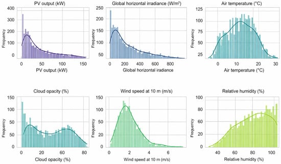
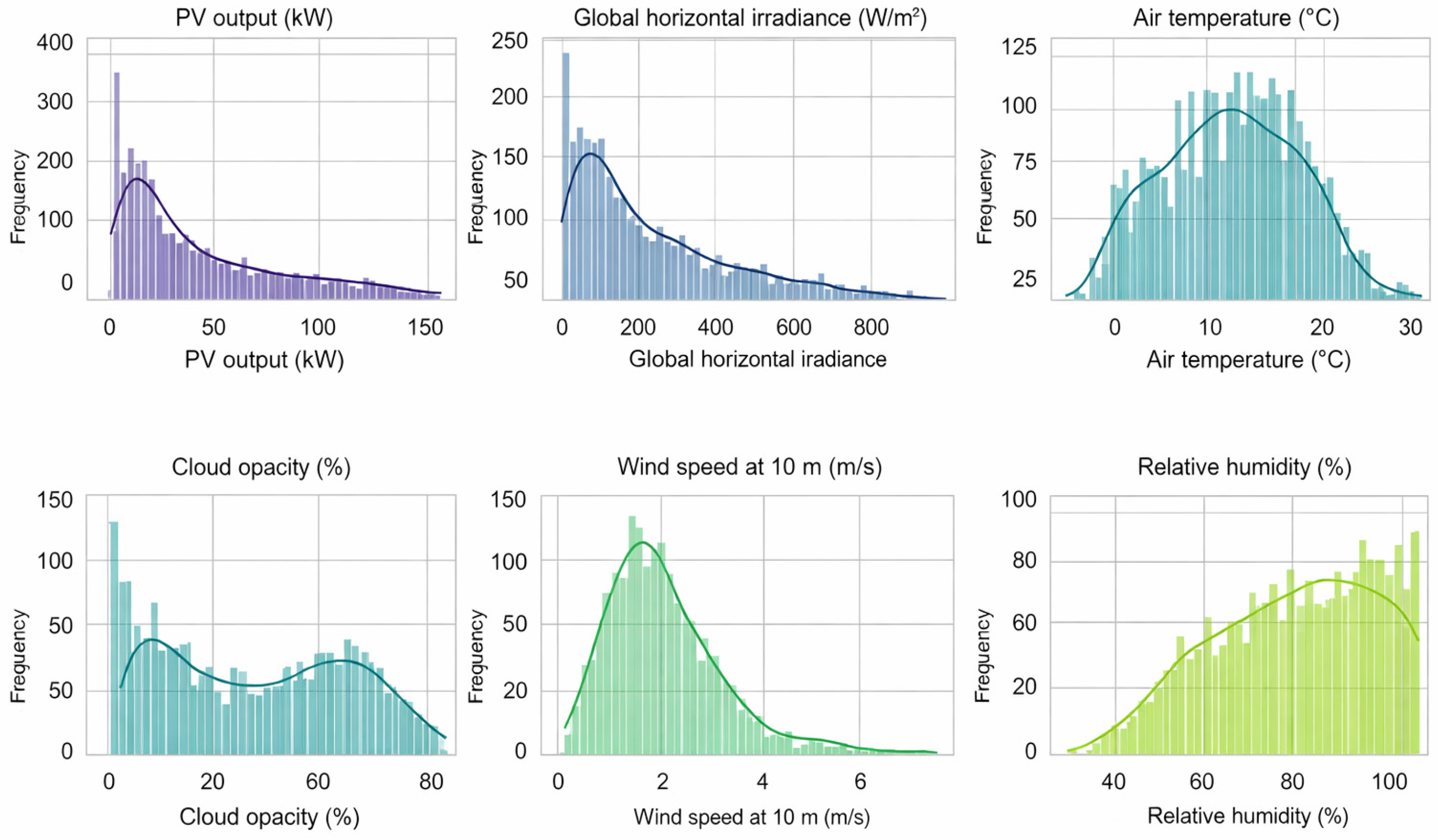
Figure 1 illustrates the distribution of the key meteorological and PV production variables in the dataset. As shown, PV output and global horizontal irradiance (GHI) exhibit a right-skewed distribution, reflecting the natural dominance of low or moderate irradiance values and fewer hours of peak solar production. Air temperature follows an approximately symmetric distribution around its mean, while the wind speed shows a Weibull pattern typical of measurements at low altitudes. Cloud opacity presents two distinct peaks, reflecting clear-sky and cloudy periods. Finally, relative humidity peaks at higher values, indicating the generally humid climate conditions of the site. The x-axes denote the respective measurement units (kW, W/m2, °C, %, m/s), and all distributions are shown after temporal aggregation to hourly resolution. Together, these distributions provide a concise overview of the operational and environmental variability captured in the dataset.
Figure 1.
Distribution of key meteorological and PV variables.
3. Conformal Prediction: Algorithms and Metrics
Uncertainty is an inevitable component of every predictive model, as real-world systems are managed by numerous interacting factors that are either difficult to measure or entirely unobservable. Since models, such as machine learning models, are typically built from limited data and approximations of reality, their forecasts are expectedly subject to different sources of uncertainty.
Accurate quantification of uncertainty is therefore crucial for ensuring the reliability and interpretability of machine learning models. By assessing uncertainty, we can estimate the range of possible outcomes, evaluate the confidence level associated with predictions generated by machine learning models, and support informed decision-making process in risk-sensitive domains. Uncertainty quantification (UQ) enables the assessment of the reliability and informativeness of model predictions, especially in scenarios involving highly intermittent processes, such as solar prediction. A model that cannot provide a measure of its own confidence is inherently limited in transparency and trustworthiness. In contrast, models capable of producing reliable uncertainty estimates enable stakeholders to better interpret predictions, manage risk, and increase reliance on automated decision systems.
Among existing UQ techniques, CP stands out as a robust, model-agnostic, and non-parametric approach that provides statistically valid prediction intervals with guaranteed coverage. Unlike traditional probabilistic or Bayesian approaches, CP does not require explicit assumptions about the underlying data distribution or model structure, making it particularly advantageous in complex, data-driven forecasting scenarios, such as those found in energy systems [19].
Besides CP methods designed for regression tasks that generate prediction intervals, there are also CP approaches developed for classification problems. Since the prediction of PV power output is inherently a regression task, Section 3.1 focuses on CP methods and evaluation metrics tailored to regression settings. Section 3.2 introduces the fundamental concepts of CP for classification are introduced, since OOD detection represents a specific variant of binary classification. A more detailed discussion of the OOD framework and its methodological aspects is provided in the following section.
3.1. CP for Regression
In the context of regression, a conformal predictor consists of several essential components that jointly determine how prediction intervals are constructed and their reliability assessed. It builds upon an underlying regression model that provides point predictions of the target variable, while the conformal prediction framework acts as a post-processing layer that calibrates these predictions to produce valid and adaptive uncertainty estimates without altering the base model itself. The trained base model then generates predictions on a separate portion of the training data, referred to as the calibration dataset. The discrepancies between predicted and true values in the calibration data, known as nonconformity scores, are computed and sorted to form an empirical distribution of model errors. Based on a user-defined significance level α, which determines the allowed error rate (e.g., α = 0.1 implies 90% nominal coverage), an appropriate quantile of the nonconformity score distribution is selected. Next, the base model predicts the target value for a new test input, while the α-quantile of the stored nonconformity scores from calibration defines the interval width around the point prediction. Finally, the conformal predictor outputs a prediction interval where d reflects the magnitude of uncertainty corresponding to the chosen significance level, and is a predicted value of test set. This procedure ensures that, under the assumption of data exchangeability, the generated intervals achieve valid marginal coverage [20].
The prediction interval construction described above corresponds to the basic CP approach, where a single global interval width is applied uniformly across all test samples. However, some instances are inherently more difficult to predict than others, and assigning them the same level of uncertainty may result in under-coverage or over-coverage. To improve interval quality, adaptive variants of CP adjust the interval width for points that are harder to predict. Several approaches are specifically developed for estimating how challenging a prediction may be. One common method relies on k-nearest neighbors to assess local prediction difficulty, while another, known as CP with Mondrian binning, groups data into Mondrian categories and calibrates uncertainty separately within each group. These two techniques can also be combined to take advantage of both local structure and broader data grouping.
3.1.1. CP with K-Nearest Neighbors as Difficulty Estimator
One widely used approach for adapting interval widths in regression tasks is CP with k-nearest neighbors (KNN). The core idea behind this method is that prediction uncertainty depends on how similar a new sample is to previously seen examples. If the neighborhood around a prediction point is dense and consistent, the model is likely to be more confident; conversely, sparse or highly variable neighborhoods suggest greater uncertainty, requiring wider prediction intervals [21].
Let denote the point prediction obtained from the base regression model for calibration sample , and its true target value. For each calibration sample, the absolute residual is computed as the baseline nonconformity score:
To incorporate local difficulty, the average distance to its nearest neighbors in feature space is calculated as:
where is calculated distace, and is sample from calibration dataset.
The normalized nonconformity score is then defined as:
where is a small constant used to avoid division by zero. These scores are stored and sorted to form the empirical error distribution. The nonconformity-score threshold is selected from the empirical score distribution to achieve the specified nominal coverage, which is set to 90% in this study.
Throughout the manuscript, denotes the significance level and denotes nominal coverage. For a set of calibration nonconformity scores , the finite-sample conformal quantile is defined as where denotes -th order statistic, with the index truncated at when necessary.
Then, using those nonconformity scores the prediction interval is determined just as in the basic variant of CP. The prediction interval is in this case the difficulty estimate of the test point multiplied by added and subtracted from the point prediction (Equation (4), where and stand for the prediction interval and point prediction, respectively, of test point , and is the neighbor difficulty of test point ).
3.1.2. CP with Mondrian Binning
CP with Mondrian binning extends the standard CP framework by enforcing conditional validity within predefined partitions of the input space. Instead of calibrating prediction uncertainty globally over the entire dataset, the calibration and test samples are divided into disjoint groups (bins), and separate nonconformity distributions are maintained for each group. This allows the prediction intervals to better reflect local characteristics of the data [22].
This method follows a binning strategy where calibration samples are partitioned according to specific value into a fixed number of equally populated bins. The bin thresholds derived from the calibration set are then applied to the test set, ensuring consistent membership assignment. For each bin , a conformal quantile is computed from the corresponding nonconformity scores. During prediction, the base model provides a point estimate for test sample , and the appropriate quantile value of observed bin is used to form the prediction interval (see (Equation (5)):
Since different regions of the prediction space exhibit different error behavior, this method of CP typically yields intervals that are narrower in well-predicted regimes and wider where uncertainty is inherently higher, improving adaptivity compared to basic CP. Prior work has demonstrated that such local calibration can significantly enhance overall efficiency without compromising validity.
According to the findings presented in [12], the application of the mentioned CP algorithms demonstrated that the best performance is achieved through a combination of CP with KNN as a difficulty estimator and CP with Mondrian binning and this unified approach will therefore be regarded as the state-of-the-art method in the remainder of this study.
3.2. CP for Time-Series Data
CP has been extended to the time series setting to enable reliable UQ for sequential and temporally dependent data. Unlike the classical CP framework, which relies on the assumption of exchangeability, time series data typically exhibit temporal dependence, recurring seasonal patterns, and gradual or abrupt changes in their underlying behavior. These characteristics violate exchangeability and may result in invalid coverage or overly conservative prediction intervals if standard CP methods are applied directly. To overcome these limitations, several variants of CP have been developed that explicitly account for temporal ordering and the sequential nature of the data [23].
In time series applications, these adaptations generally rely on constructing nonconformity scores using only past observations and updating them sequentially over time. Common approaches include rolling or sliding window schemes, block-based methods, and online calibration strategies, all of which ensure that prediction intervals are formed using information available up to the forecasting time. By relaxing the strict exchangeability assumption while preserving the distribution-free guarantees of CP, these methods provide a principled framework for UQ in forecasting problems with temporal dependence.
Among the proposed approaches, the ENBPI method represents a notable advancement for CP in time series settings. A key distinguishing feature of ENBPI is that it does not rely on a fixed calibration dataset, which is a common limitation of split conformal predictors. Instead, ENBPI employs a rolling mechanism that continuously updates nonconformity scores as new observations become available, making it well suited for sequential prediction tasks and evolving data-generating processes. This design allows ENBPI to efficiently utilize available data and naturally adapt to changes in prediction difficulty over time, which is particularly important in non-stationary environments. As a result, ENBPI achieves valid marginal coverage under mild assumptions while producing tighter and more responsive prediction intervals compared to traditional conformal methods. These properties make ENBPI a representative and state-of-the-art approach for uncertainty-aware forecasting in time series applications [24].
3.3. Metrics for Uncertainty Quantification
Reliable evaluation of CP models requires metrics that go beyond standard point-wise error measures and explicitly account for UQ, reliability, and adaptivity of prediction intervals. In many real-world applications, and particularly in energy systems and risk-aware decision-making, the usefulness of prediction intervals is determined not only by their empirical coverage, but also by their width, calibration properties, and consistency across different levels of prediction difficulty. Consequently, recent studies emphasize the need for a comprehensive set of evaluation metrics that jointly assess validity, efficiency, and adaptivity of uncertainty estimates rather than relying on coverage alone [8,9].
Marginal coverage remains a fundamental requirement of conformal predictors, ensuring that the true target value lies within the predicted interval with a predefined probability. However, coverage by itself is insufficient, as overly wide intervals may trivially satisfy coverage constraints while providing limited practical value. To address this limitation, sharpness-related metrics such as average interval width are commonly employed to quantify the informativeness of prediction intervals [25]. In addition, calibration-based metrics explicitly penalize predictions that fall outside the interval bounds, thereby capturing the magnitude of miscoverage and its dependence on the chosen significance level.
Furthermore, in adaptive CP methods, interval widths vary across samples to reflect differences in prediction difficulty. Evaluating such adaptivity requires metrics that assess how well coverage is preserved across intervals of different sizes rather than only in aggregate. Size-stratified coverage and related criteria have therefore been introduced to analyze conditional performance and detect regions where uncertainty estimates may systematically fail [26]. Coverage and Breach assess the validity of the prediction intervals, Sharpness measures their efficiency, and CWC provides a combined assessment of coverage and interval width. Together, these complementary metrics enable a concise evaluation of interval reliability and informativeness.
Motivated by their relevance to uncertainty-aware forecasting, this study evaluates prediction-interval performance using Coverage, Breach, Sharpness, and the Coverage Width-Based Criterion. Together, these metrics provide a concise assessment of interval validity and efficiency.
3.3.1. Coverage
Coverage measures the proportion of test datapoints for which the true value lies within the corresponding prediction interval and represents the primary validity criterion of CP:
where denotes the indicator function. In this setting, it is used to evaluate whether the observed target value lies within the predicted conformal interval for each test instance. By averaging the indicator values across the test set, the empirical coverage of the conformal predictor is obtained. Here, denotes the true observed value for test point , and represent the lower and upper bounds of the prediction interval, respectively, and is the total number of test samples. For a valid CP model, the empirical coverage should be close to the nominal level
3.3.2. Breach
The breach metric explicitly penalizes under-coverage by measuring the deviation from the target coverage level
If the achieved coverage is equal to or higher than , the breach is zero. Otherwise, the breach quantifies the magnitude of the shortfall. Lower values are preferred, as they indicate better adherence to the desired confidence level.
3.3.3. Sharpness
Sharpness evaluates the efficiency of the prediction intervals by measuring their average width
Narrower intervals correspond to higher sharpness and more informative predictions, provided that adequate coverage is maintained. Sharpness is commonly used as a key efficiency metric in interval forecasting and UQ.
3.3.4. Coverage Width-Based Criterion
The Coverage Width-Based Criterion (CWC) is a composite metric that jointly evaluates empirical coverage and average interval width. Its objective is to reward narrow, informative intervals while penalizing deviations from the nominal coverage level.
where MWS denotes the mean width score of the prediction intervals, is the empirical coverage probability, and represents the nominal confidence level. The parameter controls the strength of the penalty applied when the empirical coverage deviates from the desired level.
Through its exponential penalty term, CWC strongly discourages models that achieve narrow intervals at the expense of insufficient coverage, while assigning higher scores to methods that simultaneously maintain adequate coverage and small interval widths. As such, CWC provides a concise and informative summary measure for comparing conformal prediction models in uncertainty-aware forecasting tasks.
3.4. CP for Classification
In classification problems, CP provides a framework for constructing prediction sets with guaranteed coverage, rather than outputting a single class label. Instead of returning only the most probable class, a conformal classifier produces a subset of labels that contains the true class with a predefined probability defined by , denotes the significance level [8,9]. In this context, the significance level represents the tolerated error rate, while corresponds to the confidence level of the prediction set.
To construct conformal prediction sets, a conformity score function must be defined, which quantifies how well an input sample aligns with a candidate class label . Higher values of indicate stronger conformity between the sample and the assigned label. In practice, a common choice for classification tasks is the softmax probability assigned by the base classifier to class . Although such scores reflect the model’s confidence, they are often miscalibrated, and conformal prediction serves as a calibration layer that transforms them into prediction sets with guaranteed coverage.
For this conformal setting, data are partitioned into a proper training set and a calibration set of size . After training the base classifier on , conformity scores are computed on the calibration samples as , for . A threshold is then determined as the empirical )-quantile of these scores. To ensure finite-sample validity, the quantile level is adjusted as
so that the resulting threshold accounts for the finite size of the calibration set and preserves the desired coverage guarantee.
For a new test sample , conformity scores are computed for all candidate classes The conformal prediction set is then defined as
By construction, the prediction set satisfies the marginal coverage property
under the exchangeability assumption between calibration and test samples. This guarantee holds on average over different calibration sets and test points. The size of reflects predictive uncertainty: smaller sets indicate confident predictions, whereas larger sets arise when the classifier assigns comparable conformity scores to multiple classes or when the input sample is inherently difficult to classify. In this way, conformal classification provides an interpretable and distribution-free framework for uncertainty-aware decision-making.
To evaluate CP in the classification setting, we employ standard performance metrics commonly used in binary classification. This evaluation framework is particularly appropriate in the context of OOD detection, which constitutes a specific case of binary decision-making, where instances are categorized as either in distribution or out of distribution. Accordingly, performance is assessed using FPR and False Negative Rate (FNR), which quantify the proportions of incorrectly classified negative and positive samples, respectively. Complementary measures include True Positive Rate (TPR), also referred to as recall or sensitivity, and True Negative Rate (TNR), or specificity, which capture the ability of the model to correctly identify positive and negative instances.
In addition, we report precision, which reflects the reliability of positive predictions, and overall accuracy, which measures the proportion of correctly classified samples across both classes. To provide a balanced assessment in scenarios where class distributions may be skewed, the F1 score is considered as the harmonic mean of precision and recall. Finally, the Area Under the Receiver Operating Characteristic Curve (AUROC) is used to evaluate the discriminative capability of the model independently of a fixed decision threshold, summarizing the trade-off between TPR and FPR across all possible thresholds [27].
4. Proposed Approach
This section introduces the proposed framework for uncertainty-aware PV power forecasting in non-stationary environments. It begins with the formulation of CP for time series using the ENBPI algorithm, followed by a conformal approach to OOD detection based on statistical hypothesis testing. The section concludes with the integration of these components into a unified pipeline with an adaptive retraining strategy designed to handle evolving data distributions.
4.1. CP for Time-Series Forecasting of PV Data
Effective application of CP to time series forecasting requires a preprocessing pipeline that preserves temporal dependencies while enriching the feature space with informative exogenous variables. In the context of PV power generation, this involves integrating production data with meteorological observations and constructing time-based features that capture inherent periodic patterns. Accordingly, the preprocessing pipeline was designed to preserve the temporal structure of PV production data while enriching the feature space with relevant meteorological and calendar-based information. The raw dataset consists of hourly PV active power measurements for the year 2023, which were merged with corresponding hourly meteorological observations using timestamp alignment. All records were indexed by datetime to ensure strict chronological ordering throughout the analysis.
Following the data integration step, several time-based explanatory variables were constructed in order to capture periodic patterns inherent to PV generation. Specifically, the week of year, day of week, and hour of day were extracted from the timestamp and included as additional predictors. These variables allow the model to account for daily and seasonal periodicity without explicitly imposing parametric assumptions on the temporal structure.
Importantly, no separate calibration set was introduced. Unlike split conformal methods, the ENBPI algorithm does not require an explicit division into training and calibration subsets. Instead, calibration is performed internally through a rolling update of nonconformity scores during the sequential prediction process. This design allows more efficient use of available data while maintaining valid coverage guarantees under temporal dependence.
The ENBPI algorithm constructs sequential, distribution-free prediction intervals without requiring data-splitting. To handle temporal dependencies during the training phase, ENBPI utilizes a block bootstrap procedure to train bootstrap models. Each bootstrap sample preserves local temporal structure, making the procedure suitable for time-series forecasting. The core mechanism of ENBPI relies on constructing leave-one-out (LOO) ensemble estimators. By aggregating bootstrap estimators that have already been trained, it scales efficiently to produce arbitrarily many sequential prediction intervals [24].
Denoting the resulting estimators by , the aggregated predictor is defined as
Residuals are estimated using out-of-bag predictions in order to avoid optimistic bias. For each training observation, the corresponding residual is computed as
where denotes the prediction obtained by aggregating only those bootstrap models that were not trained on the observation. The empirical distribution of residuals serves as a calibration distribution.
Let denote the empirical (-quantile of these residuals. The ENBPI prediction interval for a new input is then constructed as
where is an adaptive scaling parameter chosen to stabilize empirical coverage while controlling interval width and creating an asymmetric prediction interval instead of symmetric interval as in other described CP methods.
ENBPI establishes explicit theoretical bounds on both marginal and conditional coverage gaps, ensuring they asymptotically converge to zero without requiring data exchangeability. These guarantees rely on two assumptions: a stable error process with bounded mixing properties and a sufficiently accurate regression learner. In our implementation, these assumptions are strictly addressed. The Block Bootstrap with an experimentally determined length parameter effectively preserves the temporal dependency of the error process, while the hyperparameter-optimized Random Forest ensures that the mean squared error of the LOO estimates vanishes as the sample size increases. Consequently, the proposed pipeline provides asymptotically valid conditional coverage, minimizing the deviation from the target confidence level even in non-stationary environments.
No additional smoothing or recalibration procedures were applied to the conformal prediction intervals. The intervals were evaluated directly as produced by the ENBPI algorithm. The only post-processing operation consisted of restricting the prediction interval bounds to the physically feasible range of PV power output, enforcing non-negativity and a maximum value equal to the installed capacity. This constraint ensures physical consistency of the prediction intervals without altering their conformal calibration mechanism.
4.2. Conformal OOD Detection
COOD is addressed in this work as a problem of anomaly detection, where the objective is to identify input samples that deviate from the distribution of data used for model development. In this setting, the detector is trained exclusively on in-distribution (ID) data, representing normal system operation and is subsequently applied during inference to identify samples that are statistically inconsistent with the training distribution. Such an approach is particularly suitable for PV power forecasting systems, where abnormal conditions may arise due to sensor faults, communication errors, or unexpected environmental conditions.
In many OOD detection approaches, the detection threshold must be selected manually based on heuristic choices or empirical tuning. Such a procedure does not provide statistical guarantees regarding the resulting FPR. Within this framework, CP provides a principled approach for constructing statistically valid decision rules for OOD. Conformity scores obtained on calibration data are used to define a detection threshold through a user-specified significance level, which directly controls the expected FPR [28].
Here, a conformity score function is used to quantify the agreement between a test sample and the ID training data. The conformity score is derived from the anomaly score produced by the underlying detection model and is defined as
so that lower conformity scores indicate weaker agreement with the ID data and therefore a higher likelihood that the sample is out of distribution.
The detection procedure can be interpreted as a hypothesis testing problem [8], where the null hypothesis states that a sample originates from the ID data. Statistical evidence against this hypothesis is quantified through conformal p-values computed using conformity scores from a calibration dataset. For a test sample marginal conformal p-values are defined as
where denotes the size of the calibration set. This formulation includes a finite-sample correction that prevents overly optimistic p-value estimates [29].
Small p-values indicate that the conformity score of the test sample is unusually low compared to the calibration set, suggesting that the sample is unlikely to originate from the ID data. A sample is therefore classified as OOD whenever .
Under standard conformal assumptions, this decision rule guarantees marginal control of the false positive rate:
meaning that the proportion of ID samples incorrectly identified as OOD does not exceed the chosen significance level on average. This property is particularly important in operational settings, where excessive false positives may reduce the practical usability of the detection system.
Since each incoming observation is evaluated individually using a fixed calibration dataset, the resulting sequence of hypothesis tests becomes statistically dependent [30]. In such cases, marginally valid p-values may still be overly optimistic [29], which can lead to inflated false positive rates.
To address this issue, marginal p-values are adjusted to achieve calibration-conditional validity (CCV) [29]. This is accomplished by applying an adjustment function
where is value between 0 and 1 and this represent a monotonic correction function derived from the conformity scores of the calibration dataset. The resulting p-values satisfy the CCV condition
where represent a tolerance level for the validity guarantee.
Although several adjustment methods can be applied to obtain CCV [29], in this work only the Simes correction is used, as it demonstrated the best empirical performance on energy system datasets with similar statistical properties [31]. The adjustment function is defined as a piecewise-constant mapping
where the threshold sequence is constructed so as to ensure conservative p-value estimates and reliable FPR control under dependence within the calibration dataset [29].
4.3. Overall OOD-CPAR Algorithm
The proposed OOD-CPAR framework integrates CP for time series forecasting with COOD detection into a unified pipeline for reliable PV power modeling. The method combines an ENBPI-based conformal regression model for constructing prediction intervals with a COOD detection module that identifies distribution shifts and triggers model retraining when necessary, while maintaining a low FPR in order to avoid unnecessary retraining.
During the training phase, both components follow a unified data-driven procedure. Historical data are first preprocessed and used to train the ENBPI module, where a Random Forest base model is fitted using block bootstrap resampling, and ensemble residuals are computed to construct prediction intervals. In parallel, the COOD component is trained by fitting an anomaly detection model on ID data and computing conformity scores on a calibration subset. Although a synthetic dataset is used in the evaluation phase of the COOD module, this choice is motivated solely by the ability to explicitly label samples as ID and OOD, enabling controlled and quantitative assessment of detection performance; in practical deployment, the framework assumes a common data source for both components.
In the inference phase, each incoming data point is first preprocessed and passed through the COOD module. An anomaly score is computed and transformed into a conformity score, which is then used to calculate marginal p-values. These p-values are further adjusted using the Simes correction to obtain calibration-conditionally valid p-values. Based on the resulting value and a predefined significance level α, the sample is classified as either ID or OOD.
This decision is further refined through a retraining condition applied to detected OOD samples. Rather than triggering retraining immediately, the proposed approach accumulates such samples over time. Each detected OOD point is temporarily stored, while the ENBPI model continues to produce point predictions and corresponding prediction intervals. Retraining is initiated only when the number of accumulated OOD samples exceeds a predefined threshold, indicating a persistent distribution shift rather than isolated deviations.
Once an OOD sample is detected, a retraining condition is evaluated based on the accumulation of such samples over time. If the condition is not yet satisfied, the sample is temporarily stored and treated within the standard prediction pipeline, where the ENBPI model generates the corresponding prediction intervals. When the predefined threshold on the number of detected OOD samples is reached, all samples observed since the last retraining step are incorporated into the training set, and both the ENBPI and COOD components are updated accordingly. The triggering sample is then re-evaluated under the updated models: if it is classified as ID, the standard prediction process resumes, whereas if it remains OOD, it is retained as such while still producing prediction intervals. This strategy ensures that retraining is not triggered by isolated anomalies, thereby reducing unnecessary updates, while still allowing the framework to adapt effectively to sustained distributional changes.
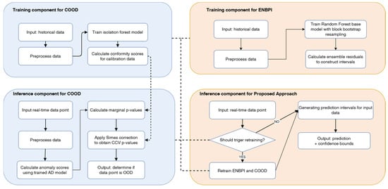
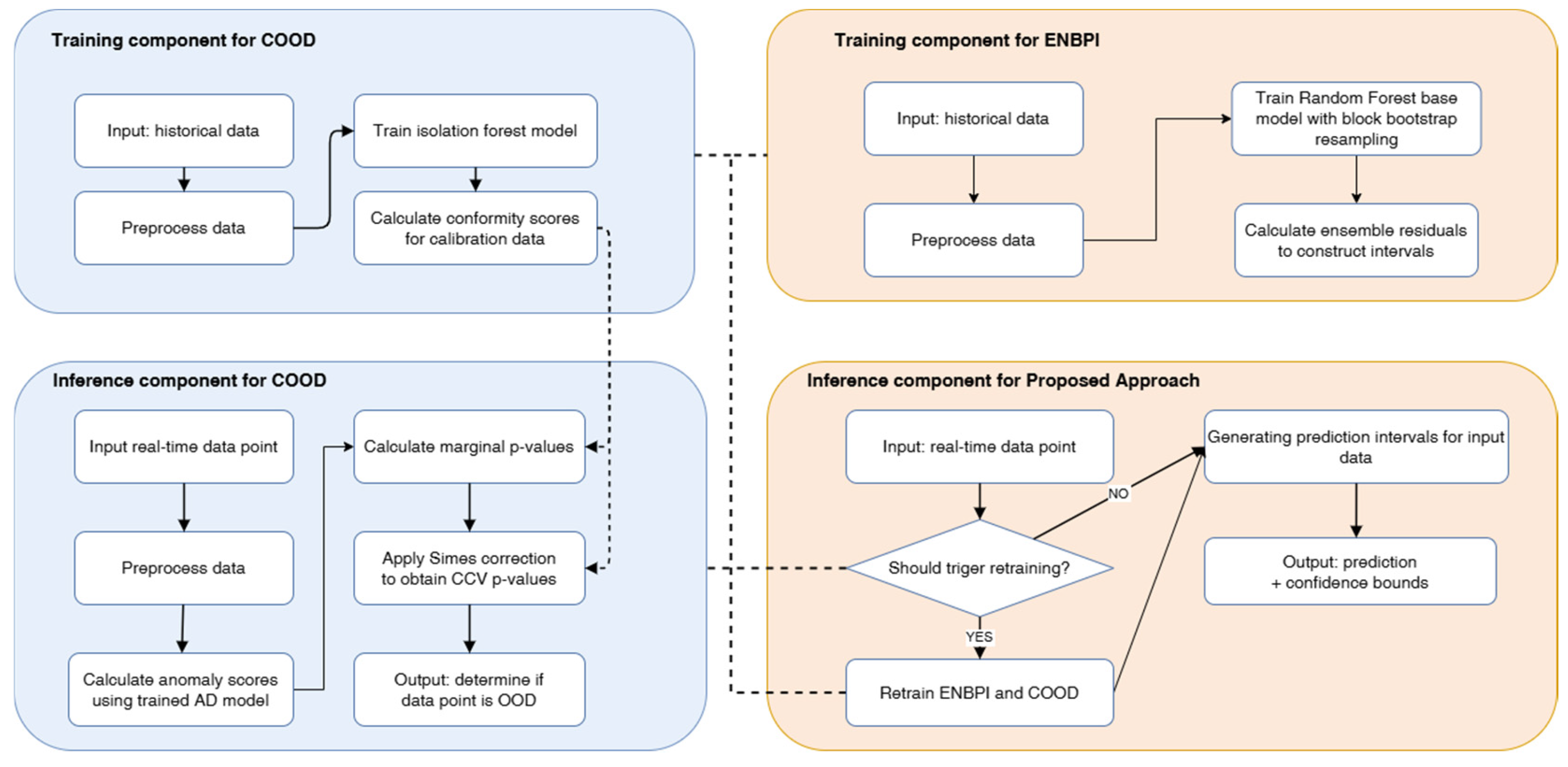
Figure 2 illustrates the overall algorithm of the proposed framework, where solid lines represent the primary data flow, while dashed lines denote control and information exchange between components. During training, conformity scores computed within the COOD module are transferred to the inference stage and used as a calibration reference for p-value estimation. In the inference phase, the COOD module evaluates each incoming sample and outputs a decision on whether the sample is classified as ID or OOD. This information is then propagated to the decision block of the proposed approach, where it is not used to trigger retraining immediately, but rather accumulated until the number of consecutively detected OOD samples reaches the OOD trigger size. Only upon meeting this condition is retraining activated, which initiates a feedback loop updating both the ENBPI and COOD components.
Figure 2.
Overall algorithm.
5. Results
This section first evaluates the ENBPI-based conformal prediction method, followed by the COOD detection framework. Finally, the performance of the proposed integrated two-stage methodology is assessed. This evaluation follows an ablation-style strategy, where the individual components are first tested independently before evaluating the complete two-stage framework.
5.1. ENBPI Performance Evaluation and Sensitivity Analysis
As the first step of the component-wise evaluation, this section assesses the EnbPI uncertainty-quantification component independently of OOD detection and adaptive retraining. Subsequently, the performance of the proposed ENBPI-based approach is compared against SOTA methods. Finally, the robustness of the proposed method is examined by analyzing how its performance varies under different train–test splits and significance levels α.
The used PV production dataset was divided into seasonal subsets in order to mitigate the influence of seasonal variability in solar power generation. Each season was treated as an independent dataset, enabling a consistent evaluation under relatively homogeneous operating conditions.
5.1.1. Residual Window Length Selection
The performance of the ENBPI method depends on the choice of the residual window length, which determines the number of past residuals used for updating prediction intervals. In order to evaluate the influence of this parameter, experiments were conducted for seven different window lengths: 24, 72, 168, 336, 504, 540, and 720 h. For each configuration, prediction intervals were computed separately for all seasons. The results were summarized using the average Coverage and Sharpness values reported in Table 1.
Table 1.
Average Coverage and Sharpness for Different Residual Window Lengths in ENBPI.
The results indicate a clear trade-off between interval reliability and interval width. Bold values highlight the selected residual window length, which provides the best balance between Coverage and Sharpness and is therefore used in the subsequent experiments. Small residual window lengths (24–168 h) produce relatively narrow prediction intervals but lead to systematic under-coverage. For example, the smallest window length (24 h) achieves the lowest average sharpness but provides insufficient coverage (0.851), significantly below the target level of 0.9. Increasing the window length improves calibration, resulting in a gradual increase in coverage.
Moderate window lengths between 336 and 540 h provide the best compromise between coverage and sharpness. In particular, a window length of 540 h yields coverage closest to the nominal level (0.896) while maintaining moderate interval width. Compared to shorter window lengths, this configuration substantially improves calibration without excessive increase in sharpness.
Very large window lengths, such as 720 h, produce the highest coverage (0.906), exceeding the nominal level and indicating conservative prediction intervals. Although the coverage is improved, the corresponding increase in sharpness suggests wider prediction intervals without a proportional gain in reliability.
5.1.2. Comparison with SOTA CP Methods
In this section, the proposed ENBPI-based time-series CP model (M4) is compared with three baseline approach, including an approach that represents the current SOTA in the literature:
- M1—CP with KNN
- M2—CP with Mondrian binning
- M3—CP with KNN and Mondrian binning [12]
To eliminate the influence of seasonal variability in photovoltaic production, the evaluation was performed separately for winter, spring, summer, and autumn datasets. Within each seasonal dataset, a chronological train–test split was performed to prevent information leakage. Specifically, the first nine twelfths of the observations were assigned to the training set, while the remaining three twelfths were reserved for out-of-sample evaluation. This temporal split preserves the sequential nature of the forecasting problem and reflects realistic deployment conditions in which future values are predicted using past observations only. The comparison includes the following performance metrics: Coverage, Breach, Sharpness and CWC. The seasonal results are presented in Table 2, Table 3, Table 4 and Table 5.
Table 2.
Winter performance comparison.
Table 3.
Spring performance comparison.
Table 4.
Summer performance comparison.
Table 5.
Autumn performance comparison.
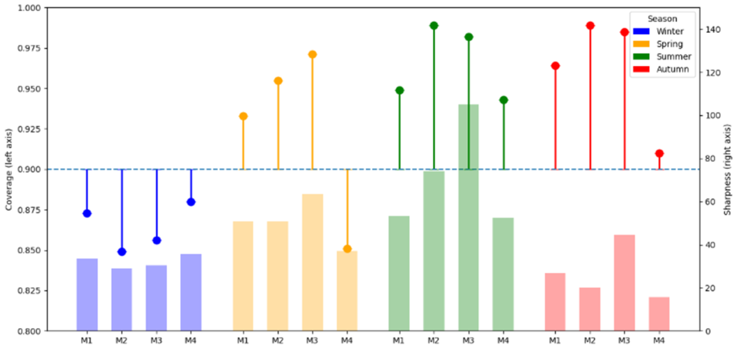
Figure 3 illustrates the relationship between coverage and sharpness across all methods and seasons. The markers represent achieved coverage values, while vertical error bars indicate the deviation from the target coverage level. The bar plots represent the corresponding sharpness values.
Figure 3.
Coverage Deviation and Sharpness by Method and Season.
Figure 3 illustrates the fundamental trade-off between coverage and interval width. Methods achieving higher coverage values typically produce wider prediction intervals, whereas narrower intervals are associated with lower coverage. While SOTA methods achieve higher coverage in some seasons, this is obtained at the cost of significantly wider prediction intervals.
During winter, the ENBPI model achieves the highest coverage (0.88), closely matching the target value while maintaining competitive interval widths. Although M2 and M3 produce slightly narrower intervals, they exhibit lower coverage and higher deviation from the target level. In spring, the SOTA methods achieve very high coverage values, reaching up to 0.971 for M3. However, this result is associated with substantially wider prediction intervals. The ENBPI model achieves lower coverage (0.851), but with significantly narrower intervals compared to all competing methods. During summer, all methods achieve coverage values close to or above the target level. ENBPI maintains one of the smallest interval widths (52.432), substantially narrower than those obtained by Mondrian-based methods, particularly M3, which produces extremely wide intervals. In autumn, ENBPI produces the narrowest prediction intervals among all methods while maintaining coverage close to the target level. Although M2 and M3 achieve very high coverage values, this again comes at the cost of wider intervals.
Across all seasons, the ENBPI model demonstrates the most balanced performance between reliability and interval efficiency. This observation is further supported by the CWC, which jointly evaluates coverage and interval width by penalizing deviations from the nominal confidence level. ENBPI consistently achieves more favorable CWC values, indicating a better trade-off between calibration and sharpness compared to the SOTA methods. While some competing approaches attain higher coverage in individual seasons, this is generally achieved through overly conservative, wider intervals. In contrast, ENBPI maintains coverage levels close to the target while avoiding unnecessary interval expansion, thereby providing a more efficient and practically relevant solution for PV power forecasting.
5.1.3. Training-Test Split Analysis
An important configuration parameter in the ENBPI algorithm is the ratio between the training and test sets. In order to assess the sensitivity of the proposed approach to this parameter, four different train–test ratios were investigated: 11/1, 10/2, 9/3, and 8/4. These ratios correspond to an analogy in which a full year is divided into twelve months, although the actual partitions were applied to seasonal datasets. The performance of each configuration was evaluated using coverage and sharpness metrics. The obtained results for the mentioned metrics are shown in Table 6 for Coverage and Table 7 for Sharpness.
Table 6.
Test Set Coverage Results for Different Train–Test Splits in ENBPI Evaluation.
Table 7.
Test Set Sharpness Results for Different Train–Test Splits in ENBPI Evaluation.
The coverage results indicate that the 9/3 train–test split provides the most consistent performance across seasons, achieving the best coverage values in winter and summer. In contrast, the remaining configurations either exhibit lower average coverage (10/2 and 8/4) or noticeable deviations from the target level despite larger training sets (11/1). The sharpness results further highlight the sensitivity of the proposed approach to the train–test split, with the 9/3 configuration yielding the narrowest prediction intervals in spring and autumn. Overall, these findings suggest that the performance of the ENBPI model is influenced by the choice of the train–test ratio, with the 9/3 split offering the most favorable balance. In addition, this configuration enables direct comparability with SOTA CP approach, where the ratio between the combined training and calibration sets and the test set typically corresponds to approximately 3:1, which is equivalent to the 9/3 partition used in this work.
5.1.4. Effect of Significance Level on ENBPI Performance
The significance level is a key parameter of the ENBPI method, directly controlling the nominal coverage level and the width of prediction intervals. In order to evaluate the influence of on interval quality, four values were considered: α ∈ {0.05, 0.1, 0.15, 0.2}. The experiments were conducted separately for each season using the 9/3 train–test split. Table 8 presents the obtained results in terms of average coverage and sharpness for different values of alpha.
Table 8.
Average Coverage and Sharpness of ENBPI for Different Significance Levels α.
The results demonstrate that the empirical coverage closely follows the theoretical target coverage level. Bold values highlight the selected significance level , which provides the target coverage level while maintaining reasonably narrow prediction intervals and is used in the subsequent experiments. For the achieved coverage is approximately 0.95 across all seasons, while for the coverage is close to the target value of 0.9. Increasing α further results in progressively lower coverage values, approaching the expected levels of 0.85 and 0.8 for and , respectively. This behavior confirms the proper calibration properties of the ENBPI method.
As expected, the sharpness of the prediction intervals decreases with increasing alpha. Lower values produce wider intervals with higher sharpness values, while larger values result in narrower intervals. For the intervals become substantially wider indicating reduced interval efficiency despite high coverage. Among the evaluated configurations, α = 0.1 provides the most favorable trade-off between coverage and sharpness.
5.2. Detection of Distribution Shifts with COOD Detector
In this subsection, we evaluate the performance of the proposed COOD detection framework in identifying distribution shifts in PV power generation data. As the second step, the OOD detector is evaluated independently using controlled synthetic OOD samples with known labels. For this purpose, a synthetic dataset was generated using the Helioscope simulator [32]. The use of a synthetic dataset is motivated by the need for controlled evaluation, as real-world PV datasets typically do not provide explicit labels indicating whether a sample belongs to the ID or OOD regime. In contrast, synthetic data enables direct control over the data-generating process, allowing us to explicitly define and label ID and OOD samples. A detailed model of the real PV power plant used in this study was constructed, incorporating all relevant physical characteristics of the panels and inverters. Based on this model, one year of hourly production data was simulated using meteorological inputs derived from historical records available within the simulator.
The resulting dataset includes key features GHI, DHI, solar angle, air temperature, albedo, and predicted grid power. This dataset was used to train the OOD detection model, where all samples were considered as ID. The data were split into training and calibration sets using a 90:10 ratio, respectively.
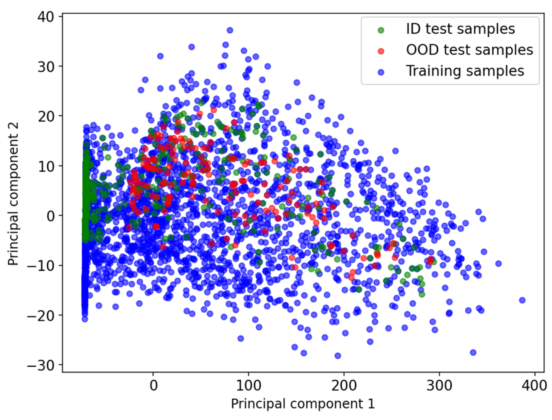
To evaluate the OOD detection capability, a test set was constructed from a representative summer month (September), selected to ensure sufficiently active PV generation throughout the period. The first half of the month was retained as ID data, while the second half was modified to simulate distribution shift. This was achieved by applying a multiplicative soiling coefficient to the output power, which resulted in a reduction in the generated power to 60%, while leaving the remaining features unchanged. This step effectively reduced the generated power and emulating the impact of panel dirtiness. In this way, the test set contains both ID and OOD samples under controlled conditions. A two-dimensional PCA projection of the training data, ID test samples, and artificially generated OOD samples is shown in Figure 4. The visualization indicates that even a significant distribution shift induced by simulated soiling is not easily separable, as OOD samples largely overlap with ID data in the feature space.
Figure 4.
PCA visualization of the feature space for training data and both ID and OOD test samples.
We first assess the baseline performance of the anomaly detection model, noting that the OOD detection task is addressed through an anomaly detection framework, where ID samples correspond to normal behavior and OOD samples are treated as anomalies. Specifically, an Isolation Forest classifier with automatically determined contamination and default hyperparameters is employed. The results indicate strong discriminative capability, with a high recall and AUROC, but at the cost of a relatively high FPR, which may lead to excessive false positives in practical applications.
Next, we evaluate the COOD detection framework based on marginal p-values. While this approach significantly reduces the FPR compared to the baseline model, it does so at the expense of a substantial increase in FNR. This behavior is expected, as the primary objective of the conformal framework is to control the FPR at a predefined significance level (in this case, α = 0.1), leading to a conservative detection strategy. Importantly, the AUROC remains largely unchanged, indicating that conformalization primarily affects the decision threshold rather than the underlying ranking capability of the detector
Finally, we apply the Simes correction to obtain calibration-conditionally valid p-values. The results show that this adjustment further reduces the FPR compared to marginal p-values, leading to fewer false positives and more stable operation. At the same time, the AUROC remains practically unchanged, confirming that the discriminative ability of the detector is preserved. Additionally, improvements in accuracy and precision are observed, highlighting the benefit of calibration-conditional adjustment in achieving a better balance between reliability and detection performance. The quantitative results are summarized in Table 9.
Table 9.
Comparison of OOD detection methods.
The marginal and Simes-corrected decisions substantially reduce the FPR, which was an important design objective because false OOD alarms may trigger unnecessary and computationally expensive model retraining. However, the FNR of 0.8038 and recall of 0.1962 show that this conservative behavior comes at the cost of missed OOD samples and potentially delayed adaptation. Thus, the selected operating point prioritizes avoiding unnecessary retraining over sample-level detection sensitivity. This trade-off can be adjusted through the significance level α, increasing α makes the detector less conservative and typically reduces the FNR, but increases the FPR and may consequently lead to more frequent retraining. The operational effect of this trade-off is evaluated in Section 5.3, where the detector is integrated with the adaptive retraining mechanism.
5.3. Evaluation of the Proposed OOD-CPAR Framework
This subsection examines the behavior of the proposed OOD-CPAR framework, with the goal of illustrating how the integration of OOD detection and adaptive retraining influences predictive reliability. The evaluation of the complete OOD-CPAR framework was performed using the measured dataset described in Section 2, with controlled synthetic distribution shifts introduced according to Section 5.2. The analysis emphasizes the practical impact of introducing retraining into a conformal prediction pipeline, particularly in comparison to a static ENBPI model operating without adaptation.
The baseline ENBPI model is compared against the OOD-CPAR framework under different retraining configurations. The retraining mechanism is controlled by a parameter defining the minimum number of consecutively detected OOD samples required to trigger retraining, which directly determines the sensitivity of the system to distribution shifts and results are summarized in Table 10.
Table 10.
Performance comparison of baseline ENBPI and OOD-CPAR under different retraining configurations.
The baseline ENBPI model achieves a coverage of 0.853, which falls below the desired level (1 − α = 0.9), indicating that without adaptation the model is unable to maintain reliable uncertainty estimates under distribution shift. In contrast, the OOD-CPAR framework consistently restores coverage across a broad range of retraining configurations, with most settings achieving values close to or slightly above the target level.
A clear trade-off emerges when considering execution time. Frequent retraining (small trigger sizes) leads to a substantial increase in computational cost, whereas larger trigger sizes significantly reduce execution time. Intermediate configurations (e.g., trigger sizes between 10 and 40) provide a favorable balance, achieving reliable coverage with considerably lower computational overhead, making them particularly suitable for practical deployment.
In terms of interval efficiency, the sharpness metric reveals a more nuanced behavior. While one might expect a monotonic relationship where improved coverage is achieved at the cost of wider intervals, the results indicate that sharpness does not vary linearly with coverage. Instead, interval widths fluctuate across configurations, reflecting the interaction between retraining frequency and local data characteristics. Frequent retraining adapts the model more closely to recent data, which can lead to either narrower or wider intervals depending on the variability of the updated data regime, while less frequent retraining results in more stable but less adaptive interval widths. This highlights that the proposed framework does not simply trade sharpness for coverage, but dynamically adjusts interval width in response to underlying distributional changes.
Overall, the results demonstrate that the OOD-CPAR framework effectively enhances the robustness of conformal prediction under distribution shift. By combining statistically controlled OOD detection with adaptive retraining, the approach restores coverage and reduces false positives while providing explicit control over computational cost. The results further indicate that the framework achieves a flexible balance between reliability and interval efficiency, adapting both coverage and interval width to evolving data conditions.
6. Conclusions
The expanding role of solar PV generation in modern power systems demands forecasting approaches that combine high point prediction accuracy with reliable uncertainty quantification. This paper proposed a novel OOD-CPAR to address the critical limitations of standard CP methods in real-world environments characterized by evolving data distributions.
First, to overcome the restrictive data exchangeability assumption, we successfully applied the ENBPI framework to sequential PV production data. Comprehensive seasonal evaluations demonstrated that the ENBPI approach consistently achieves a superior trade-off between statistical reliability (coverage) and interval efficiency (sharpness) compared to state-of-the-art CP techniques, such as KNN and Mondrian binning. While existing methods often achieve target coverage at the expense of impractically wide intervals, the proposed approach maintains nominal coverage while avoiding overly conservative behavior.
Second, we introduced the first COOD detection mechanism explicitly tailored for solar forecasting. By framing OOD detection as a hypothesis testing problem and applying the Simes correction to compute calibration-conditionally valid p-values, the proposed method rigorously controls the FPR while preserving the underlying anomaly detector’s discriminative capability. This prevents too frequent and unnecessary retraining in the overall framework.
Finally, the integration of COOD detection with an adaptive retraining strategy enables the framework to dynamically respond to sustained distribution shifts. Experimental results confirm that OOD-CPAR effectively restores coverage and significantly improves calibration under non-stationary conditions. Furthermore, by requiring a predefined accumulation of OOD samples before triggering an update, the strategy prevents unnecessary retraining, offering explicit control over computational costs.
By coupling robust time-series uncertainty quantification with mathematically grounded distribution shift awareness, this work demonstrates that theoretical coverage guarantees can be maintained in operational forecasting pipelines for renewable energy systems. Although the proposed framework shows promising results, several directions for future work remain. These include the development of more advanced retraining strategies, exploration of alternative OOD detection methods, and validation on additional real-world datasets. Furthermore, extending the framework to multi-step forecasting and other renewable energy domains represents an important avenue for further research.
Author Contributions
Conceptualization, U.I. and O.K.; methodology, U.I. and O.K.; validation, M.A.S., N.R. and Z.S.; formal analysis, U.I. and A.P.; data curation, U.I.; writing—original draft preparation, U.I. and O.K.; writing—review and editing, M.A.S., N.R. and Z.S.; visualization, U.I. and A.P. All authors have read and agreed to the published version of the manuscript.
Funding
This work has been supported by the Ministry of Science, Technological Development and Innovation of the Republic of Serbia [GN: 451-03-33/2026-03/200102] and [GN: 451-03-34/2026-03/200102].
Data Availability Statement
This article uses electricity production data from a photovoltaic plant located in southern Serbia, based on real operational measurements. Upon publication of this work, the PV generation dataset will be made publicly available at [https://github.com/UrosElfak/datasetOOD-CPAR.git, accessed on 5 May 2026]. Further inquiries can be directed to the corresponding author.
Conflicts of Interest
Author Ognjen Kundačina was employed by the Microsoft Corporation (Serbia). The remaining authors declare that the research was conducted in the absence of any commercial or financial relationships that could be construed as potential conflicts of interest.
Abbreviations
The following abbreviations are used in this manuscript:
| PV | Photovoltaic |
| CP | Conformal prediction |
| OOD | Out-Of-Distribution |
| COOD | Conformal Out-Of-Distribution |
| OOD-CPAR | Conformal Prediction framework with Adaptive Retraining |
| ENBPI | Ensemble Batch Prediction Intervals |
| FPR | False positive rate |
| GHI | Global horizontal irradiance |
| DHI | Diffuse horizontal irradiance |
| DNI | Direct normal irradiance |
| GTI | Global tilted irradiance |
| IQR | Interquartile Range |
| UQ | Uncertainty quantification |
| KNN | k-nearest neighbors |
| CWC | Coverage Width-Based Criterion |
| FNR | False Negative Rate |
| TPR | True Positive Rate |
| TNR | True Negative Rate |
| AUROC | Area Under the Receiver Operating Curve |
| ID | In-distribution |
References
- International Energy Agency. Renewables 2024, Paris, IEA, 2024. Available online: https://www.iea.org/reports/renewables-2024 (accessed on 15 January 2026).
- Rajagukguk, R.A.; Ramadhan, R.A.A.; Lee, H.-J. A Review on Deep Learning Models for Forecasting Time Series Data of Solar Irradiance and Photovoltaic Power. Energies 2020, 13, 6623. [Google Scholar] [CrossRef] [Scilit]
- Inman, R.H.; Pedro, H.T.C.; Coimbra, C.F.M. Solar forecasting methods for renewable energy integration. Prog. Energy Combust. Sci. 2013, 39, 535–576. [Google Scholar] [CrossRef] [Scilit]
- Morales, J.M.; Conejo, A.J.; Madsen, H.; Pinson, P.; Zugno, M. Integrating Renewables in Electricity Markets: Operational Problems; International Series in Operations Research & Management Science; Springer: Boston, MA, USA, 2014; Volume 205. [Google Scholar] [CrossRef] [Scilit]
- Box, G.E.P.; Jenkins, G.M.; Reinsel, G.C.; Ljung, G.M. Time Series Analysis: Forecasting and Control, 5th ed.; John Wiley & Sons: Hoboken, NJ, USA, 2015; ISBN 978-1-118-67502-1. [Google Scholar]
- Alharbi, F.R.; Csala, D. Wind Speed and Solar Irradiance Prediction Using a Bidirectional Long Short-Term Memory Model Based on Neural Networks. Energies 2021, 14, 6501. [Google Scholar] [CrossRef] [Scilit]
- Wu, K.; Peng, X.; Li, Z.; Cui, W.; Yuan, H.; Lai, C.S.; Lai, L.L. A Short-Term Photovoltaic Power Forecasting Method Combining a Deep Learning Model with Trend Feature Extraction and Feature Selection. Energies 2022, 15, 5410. [Google Scholar] [CrossRef] [Scilit]
- Vovk, V.; Gammerman, A.; Shafer, G. Algorithmic Learning in a Random World; Springer International Publishing: Cham, Switzerland, 2022. [Google Scholar] [CrossRef] [Scilit]
- Angelopoulos, A.N.; Bates, S. Conformal Prediction: A Gentle Introduction. Found. Trends Mach. Learn. 2023, 16, 494–591. [Google Scholar] [CrossRef] [Scilit]
- Jensen, V.; Bianchi, F.M.; Anfinsen, S.N. Ensemble conformalized quantile regression for probabilistic time series forecasting. IEEE Trans. Neural Netw. Learn. Syst. 2023, 35, 9014–9025. [Google Scholar] [CrossRef] [Scilit] [PubMed]
- Tajmouati, S.; Wahbi, B.E.; Dakkon, M. Applying regression conformal prediction with nearest neighbors to time series data. Commun. Stat. Simul. Comput. 2024, 53, 1768–1778. [Google Scholar] [CrossRef] [Scilit]
- Renkema, Y.; Visser, L.; AlSkaif, T. Enhancing the reliability of probabilistic PV power forecasts using conformal prediction. Sol. Energy Adv. 2024, 4, 100059. [Google Scholar] [CrossRef] [Scilit]
- Hu, J.; Luo, Q.; Tang, J.; Heng, J.; Deng, Y. Conformalized temporal convolutional quantile regression networks for wind power interval forecasting. Energy 2022, 248, 123497. [Google Scholar] [CrossRef] [Scilit]
- Wang, W.; Feng, B.; Huang, G.; Guo, C.; Liao, W.; Chen, Z. Conformal asymmetric multi-quantile generative transformer for day-ahead wind power interval prediction. Appl. Energy 2023, 333, 120634. [Google Scholar] [CrossRef] [Scilit]
- Tibshirani, R.J.; Barber, R.F.; Candès, E.J.; Ramdas, A. Conformal prediction under covariate shift. arXiv 2019, arXiv:1904.06019. [Google Scholar] [CrossRef] [Scilit]
- Yang, Y.; Kuchibhotla, A.K.; Tchetgen, E.T. Doubly robust calibration of prediction sets under covariate shift. arXiv 2022, arXiv:2203.01761. [Google Scholar] [CrossRef] [Scilit]
- Pournaderi, M.; Xiang, Y. Training-conditional coverage bounds under covariate shift. arXiv 2025, arXiv:2405.16594. [Google Scholar] [CrossRef] [Scilit]
- Solcast. Global Solar Irradiance Data and PV System Power Output Data. 2024. Available online: https://solcast.com/ (accessed on 21 September 2025).
- Borrotti, M. Quantifying Uncertainty with Conformal Prediction for Heating and Cooling Load Forecasting in Building Performance Simulation. Energies 2024, 17, 4348. [Google Scholar] [CrossRef] [Scilit]
- Manokhin, V. Practical Guide to Applied Conformal Prediction in Python: Learn and Apply the Best Uncertainty Frameworks to Your Industry Applications, 1st ed.; Packt Publishing Limited: Birmingham, UK, 2023. [Google Scholar]
- Papadopoulos, H.; Vovk, V.; Gammerman, A. Regression Conformal Prediction with Nearest Neighbours. Jair 2011, 40, 815–840. [Google Scholar] [CrossRef] [Scilit]
- Toccaceli, P.; Gammerman, A. Combination of inductive mondrian conformal predictors. Mach. Learn. 2019, 108, 489–510. [Google Scholar] [CrossRef] [Scilit]
- Stocker, M.; Małgorzewicz, W.; Fontana, M.; Taieb, S.B. A gentle introduction to conformal time series forecasting. arXiv 2025, arXiv:2511.13608. [Google Scholar] [CrossRef] [Scilit]
- Xu, C.; Xie, Y. Conformal Prediction for Time Series. IEEE Trans. Pattern Anal. Mach. Intell. 2023, 45, 11575–11587. [Google Scholar] [CrossRef] [Scilit] [PubMed]
- Gneiting, T.; Balabdaoui, F.; Raftery, A.E. Probabilistic forecasts, calibration and sharpness. J. R. Stat. Soc. Ser. B Stat. Methodol. 2007, 69, 243–268. [Google Scholar] [CrossRef] [Scilit]
- Khosravi, A.; Nahavandi, S.; Creighton, D. Construction of Optimal Prediction Intervals for Load Forecasting Problems. IEEE Trans. Power Syst. 2010, 25, 1496–1503. [Google Scholar] [CrossRef] [Scilit]
- Saito, T.; Rehmsmeier, M. The precision-recall plot is more informative than the ROC plot when evaluating binary classifiers on imbalanced datasets. PLoS ONE 2015, 10, e0118432. [Google Scholar] [CrossRef] [Scilit] [PubMed]
- Laxhammar, R.; Falkman, G. Inductive conformal anomaly detection for sequential detection of anomalous sub-trajectories. Ann. Math. Artif. Intell. 2015, 74, 67–94. [Google Scholar] [CrossRef] [Scilit]
- Bates, S.; Candès, E.; Lei, L.; Romano, Y.; Sesia, M. Testing for outliers with conformal p-values. Ann. Stat. 2023, 51, 149–178. [Google Scholar] [CrossRef] [Scilit]
- Benjamini, Y.; Hochberg, Y. Controlling the false discovery rate: A practical and powerful approach to multiple testing. J. R. Stat. Soc. Ser. B Stat. Methodol. 1995, 57, 289–300. [Google Scholar] [CrossRef] [Scilit]
- Kundacina, O.; Vincan, V.; Gojic, G.; Ninkovic, V.; Miskovic, D. Conformal anomaly detection for predictive maintenance in thermal power plants. IEEE Access 2025, 13, 39738–39752. [Google Scholar] [CrossRef] [Scilit]
- Aurora Solar. HelioScope—Commercial Solar Software. 2026. Available online: https://helioscope.aurorasolar.com/ (accessed on 18 February 2026).

Disclaimer/Publisher’s Note: The statements, opinions and data contained in all publications are solely those of the individual author(s) and contributor(s) and not of MDPI and/or the editor(s). MDPI and/or the editor(s) disclaim responsibility for any injury to people or property resulting from any ideas, methods, instructions or products referred to in the content. |
© 2026 by the authors. Licensee MDPI, Basel, Switzerland. This article is an open access article distributed under the terms and conditions of the Creative Commons Attribution (CC BY) license.