


Abstract
Smart grids with high renewable penetration are increasingly evaluated through long-horizon production simulation, but conventional decomposed simulation mainly reports energy balance and unit feasibility, while power-quality stress remains weakly quantified in the storage correction layer. This paper presents a power-quality-proxy-guided state-replay framework for renewable-rich smart grids. Instead of claiming feeder-level electromagnetic simulation, the method defines planning-level proxy indicators that can be exported by production-simulation software: a voltage-deviation proxy obtained from net-power sensitivity, a net-load ramp proxy, an inverter/charger harmonic-risk proxy, and a renewable-curtailment exposure proxy. These normalized indicators are combined into a composite score , which is then used to distinguish two storage values: charge retention during renewable-surplus voltage-rise intervals and discharge support during voltage-dip, ramp-stress, or inverter-stress intervals. A base decomposed production-simulation schedule is first obtained. The proposed layer then constructs storage accounting cycles independent of monthly and rolling-window boundaries, attaches the proxy ledger to each interval, backtracks terminal residual storage energy to low-value charging actions, and reallocates physically feasible discharge to high- intervals. The corrected storage path is projected onto power and energy limits and replayed before storage and conventional-unit states are inherited by the next monthly solve; cycles outside the replay validity envelope are escalated to full redispatch rather than counted as successful corrections. An eight-interval case reports explicit values and shows that a trajectory ending 45 MWh above the 30 MWh reference can be corrected by trimming 35 MWh of low-proxy-value charging and adding 10 MWh of discharge in two high-score intervals. A 96-interval experiment further shows that the full method reduces explicitly discarded residual energy from 214 MWh to 31 MWh, provides 128 MWh of proxy-guided support, and lowers weighted PQ-proxy exposure by 46.3%. The framework links smart-grid data analysis, renewable integration, and power-quality improvement within a traceable production-simulation workflow.
1. Introduction
1.1. Motivation: Renewable-Rich Smart Grids and Power-Quality-Aware Simulation
The transition toward renewable-rich smart grids changes the purpose of long-horizon production simulation. Planning studies no longer need only a chronological energy balance; they also need to understand whether flexible resources can support voltage stability, ramping smoothness, renewable absorption, and power-quality resilience when renewable generation and new loads fluctuate together.
A 15 min annual simulation contains 35,040 intervals. This scale is manageable for data storage but difficult for a monolithic mixed-integer model when unit commitment, ramping, reserves, storage state equations, renewable scenarios, and explicit power-quality proxy indicators are represented simultaneously.
Monthly decomposition and rolling-window optimization remain attractive because they keep the engineering software maintainable. However, the computational window is not a physical boundary. A feeder voltage fluctuation, an electric-vehicle load ramp, or a storage state trajectory can cross the same boundary that the solver uses only for convenience.
Energy storage is a key smart-grid actuator because it can absorb renewable surplus during voltage-rise or curtailment exposure and discharge during voltage-dip, ramp-stress, or inverter-stress intervals. Yet storage closure rules and state inheritance are often handled as energy-accounting issues, disconnected from the proxy indicators that motivated storage operation.
The central research question is therefore: how can a decomposed production-simulation workflow use storage not only to satisfy residual-energy accounting, but also to reduce power-quality stress caused by renewable variability and new flexible loads?
The proposed answer is a power-quality-proxy-guided storage state-replay layer. The base monthly schedule remains the primary optimization output. After the base solution is available, the replay layer audits complete storage accounting cycles, evaluates over the same intervals, identifies residual energy created by low-value charging, preserves charging that has renewable-absorption or voltage-rise mitigation value, and reallocates feasible discharge to high-score intervals.
This design uses data-driven proxy indicators to link renewable integration with voltage-fluctuation, ramping, and harmonic-risk mitigation while keeping storage correction traceable enough for engineering production-simulation reports.
The result is not a black-box rescheduling engine. It is an auditable post-solution mechanism that reports which charging actions were changed, which power-quality stress intervals received additional support, and whether the next month inherits a state that can be replayed from the corrected trajectory.
1.2. Literature Review
The first relevant stream of research concerns long-horizon production simulation and unit-commitment modeling. Unit commitment remains the standard scheduling core for planning studies because it can represent binary commitment status, startup and shutdown transitions, ramping limits, reserve requirements, and chronological economic dispatch within a unified optimization framework [1,2,3,4]. Compact and strengthened mixed-integer formulations have made repeated chronological solves more tractable, which explains their continuing use in production-simulation software. However, these formulations are mainly designed to preserve feasibility and economic consistency within a specified optimization horizon. When an annual study is decomposed into months or rolling windows, additional logic is still needed to ensure that boundary states, storage accounting cycles, and audit records remain physically replayable.
A second stream focuses on renewable-energy integration under chronological uncertainty. Studies on wind and photovoltaic variability have shown that renewable output reshapes unit commitment, dispatch, reserve use, scenario construction, and multi-stage scheduling decisions [5,6,7,8,9]. The common conclusion is that planning models must preserve time chronology rather than relying only on annual energy totals or isolated peak conditions. Nevertheless, most renewable-integration studies report energy balance, operating cost, curtailment, or flexibility adequacy as their primary outputs. The connection between those planning-level records and explicit power-quality stress indicators, such as voltage deviation, ramp pressure, inverter loading, and curtailment exposure, is still limited.
A third stream studies the role of storage in commitment, dispatch, rolling-horizon scheduling, and uncertainty management. Existing work has demonstrated that storage can hedge renewable uncertainty, coupled with thermal commitment, support frequency-related constraints, reshape microgrid dispatch, and participate in chance-constrained economic dispatch [10,11,12,13,14,15,16,17,18,19,20]. These studies provide the modeling foundation for representing storage as an active flexibility resource. Their focus, however, is usually on allocating charge and discharge within the current optimization horizon and checking terminal energy feasibility. They rarely treat a terminal residual as an auditable energy source that should be traced back to the charging intervals that created it and then classified as retained absorption value, removable low-value charging, or feasible support for later high-stress intervals.
A fourth stream comes from smart-grid control and power-quality-oriented operation. Model predictive control and distributed control studies show that storage can improve transient stability, coordinate local resources, and use forecasted operating conditions when detailed state feedback is available [21,22,23]. Power-quality-related studies further show that voltage stress, inverter-rich operation, and long-term chronological load representation should not be ignored in planning contexts [24,25,26]. These methods clarify the physical motivation for voltage- and stress-aware storage actions, but detailed feeder-level electromagnetic or harmonic models are difficult to embed directly in every interval of an annual production simulation. A planning workflow, therefore, needs simplified but interpretable proxy indicators that can be exported from ordinary simulation records.
A fifth stream evaluates storage value over long planning horizons and changing market or decarbonization contexts. These studies show that storage value depends on the generation mix, curtailment conditions, market rules, resilience requirements, and the chronological sequence of surplus and shortage events [27,28,29,30,31]. For engineering production-simulation reports, this implies that storage should be assessed not only by final state of charge or total cost, but also by the traceability and usefulness of its chronological actions. Long-term storage-value studies, however, generally do not provide a mechanism for reconciling decomposed simulation boundaries with cycle-level residual-energy attribution and power-quality-oriented support.
Taken together, the literature leaves three methodological gaps for decomposed production simulation. First, residual storage energy is often treated as a terminal boundary-accounting issue rather than as a traceable energy source. Second, storage inheritance is usually checked through terminal energy consistency, while the replayability of the complete corrected trajectory receives less attention. Third, planning-level power-quality proxies are rarely recorded in the same ledger as residual-energy correction, which makes it difficult to explain whether a storage adjustment supports renewable absorption, voltage-stress relief, ramp mitigation, or inverter-risk reduction.
This paper addresses these gaps by combining residual-energy backtracking, proxy-score construction, storage state replay, and cross-month inheritance in one auditable layer. The proposed method is positioned between feeder-level electromagnetic power-quality simulation and high-level production-cost modeling. It does not replace detailed harmonic or voltage analysis; instead, it introduces computable planning proxies into long-horizon production simulation so that high-stress intervals can be identified, storage corrections can be traced, and cases requiring full redispatch or detailed network verification can be explicitly flagged.
In this way, the proposed framework provides a practical link among smart-grid data analysis, renewable-integration assessment, power-quality-aware storage use, and engineering production-simulation software.
The following subsection summarizes the unresolved issues and contributions derived from this positioning.
1.3. Unresolved Issues and Contributions
Four unresolved issues motivate this study. First, a decomposed production simulation can pass storage and unit states between months without proving that the states are replayable from the corrected trajectory. Second, residual storage energy is often cleared at a boundary even when high power-quality proxy intervals exist inside the same cycle. Third, renewable-surplus charging, voltage deviation, ramping stress, and inverter/harmonic risk are usually audited in different modules. Fourth, annual reports rarely quantify how much storage correction reduces proxy-measured power-quality exposure rather than only reducing terminal residual energy.
Contribution 1: A power-quality-proxy-guided storage accounting cycle is introduced to decouple proxy assessment windows, rolling optimization windows, and natural-month boundaries.
Contribution 2: A transparent proxy ledger is developed from voltage deviation, ramping, inverter/harmonic risk, and renewable-curtailment indicators, and it is used to rank charge-retention and discharge-benefit actions.
Contribution 3: A proxy-oriented residual-energy allocation mechanism reallocates feasible storage discharge to high- intervals while respecting power, energy, and accounting-cycle constraints.
Contribution 4: A state replay and inheritance mechanism is used so that corrected storage trajectories and conventional-unit histories remain physically continuous across monthly solves.
Contribution 5: Case studies report discarded residual energy, proxy-guided support, weighted exposure reduction, renewable-curtailment absorption, storage-state jumps, and cross-month ramping continuity.
1.4. Paper Organization
Section 2 formulates the decomposed smart-grid production-simulation setting, defines the power-quality proxy ledger, and states the assumptions under which residual energy is identifiable. Section 3 presents the deterministic replay algorithm, residual-energy allocation procedure, computational complexity, and key properties. Section 4 describes state inheritance, audit metrics, annual-run acceptance criteria, the reproducibility data contract, stress-test design principles, software regression testing, data-quality handling, and replay-redispatch escalation. Section 5 reports the traceable example, multi-cycle experiment, ablation study, accounting-granularity sensitivity, experimental validity interpretation, transferability protocol, and practical reporting requirements. Section 6 concludes the paper.
2. Problem Formulation for Proxy-Guided Smart-Grid Production Simulation
2.1. Renewable-Rich Chronology, Smart-Grid States, and Monthly Decomposition
The modeling chain begins with the chronological records that make annual production simulation observable at an interval resolution. Adjusted demand and net demand are therefore defined before the monthly decomposition, because the optimizer, the residual-energy ledger, and the proxy-support audit all read the same demand balance.
where denotes adjusted demand at interval t; denotes original load; denotes the reserve or demand-adjustment ratio; denotes net demand after fixed schedules; denotes fixed generation from source i in set ; denotes fixed tie-line or import schedule l in set ; and denotes the interval length used when power is accumulated as energy. Mathematically, the equations first scale the raw load into adjusted demand and then subtract fixed generation and import schedules to obtain net demand. In engineering terms, they establish the common interval-level baseline used by the monthly optimizer, residual ledger, and proxy-support evaluation.
The balancing task still subtracts fixed renewable, must-run, and tie-line schedules from total demand. The difference in the formulation is interpretive: surplus and deficit records are also used later to determine whether storage charging or discharging improves renewable integration and power quality.
With the interval-level demand records fixed, the next question is how to divide a year-long chronology for computation without turning each month into a physical reset point. The monthly partition below defines solver windows while preserving the continuity required by storage and power-quality processes.
where denotes the full chronological simulation horizon, and to denote the monthly subsets used by the decomposed annual simulation. Mathematically, the expression partitions the full horizon into ordered monthly subsets. In engineering terms, it makes clear that months are solver windows inside one continuous annual trajectory.
The annual horizon is decomposed into monthly subsets for computational reasons. This decomposition does not reset the physical smart-grid state, the storage accounting cycle, or the power-quality stress process.
A state-mapping relation, therefore, connects adjacent months. In the proposed framework, this mapping must be built from the replayed storage trajectory and the inherited unit history after proxy-guided correction.
Once months are treated as computational windows, the boundary between two solves must carry an operational state package rather than a loose end condition. The following mapping specifies the information that is transferred from one month to the next after replay.
where denotes the terminal state package of month m; denotes the initial state package passed to month m + 1; and denotes the state-mapping operator that transfers replayed storage and unit states across the month boundary. Mathematically, the mapping sends the terminal state package of one month to the initial state package of the next month. In engineering terms, it is the formal place where replayed storage states and inherited unit histories are transferred.
The inherited state vector contains conventional-unit output, commitment status, storage energy, and the proxy-related flags needed by the following monthly solve.
2.2. Base Monthly Optimization and Proxy Records
For each month, a base feasible schedule is obtained before the replay layer is applied. The monthly objective still includes deficit penalties, surplus penalties, conventional-unit operating costs, and storage operating costs.
The proposed layer starts from a conventional monthly schedule, so the baseline optimization problem has to remain explicit. The objective below defines the schedule that will later be audited, corrected, and replayed instead of being replaced by a new global optimizer.
where denotes the objective value of month m; and are the deficit and surplus penalty coefficients; and are deficit and surplus variables; denotes the operating cost of conventional unit j; , , , and are the output, commitment, start-up, and shut-down arguments of that unit-cost function; denotes the storage operating cost of device k; is the storage-power argument of that cost; is the interval set of month m; is the conventional-unit set; and is the storage set. Mathematically, the objective aggregates deficit, surplus, conventional-unit, and storage operating terms over one month. In engineering terms, it defines the baseline schedule that the replay layer audits and corrects without rebuilding the whole optimizer.
The proposed layer does not require rebuilding the base optimizer. It requires the base optimizer to export storage power, storage energy, deficit, surplus, renewable-curtailment exposure, net-load ramp records, feeder-sensitivity records when available, and inverter/charger loading proxies.
The power-balance relation remains the physical accounting foundation of the model.
The replay ledger can only use quantities that are visible in the base production-simulation record. The balance equation, therefore, keeps conventional output, storage power, deficits, and surpluses in the same interval-level accounting relation.
where is the output of conventional unit j; is the storage power of device k; and are deficit and surplus variables; is net demand; and and are the conventional units and storage sets. Mathematically, the equation balances net demand using conventional output, storage power, deficit, and surplus variables. In engineering terms, the same residual deficit and surplus records later identify support targets and possible low-value charging sources.
Here, the deficit and surplus variables are retained explicitly. Later, deficit variables identify candidate support intervals, while surplus variables help determine whether earlier charging is low-value or renewable-integration-oriented.
Storage replay is meaningful only when the conventional-unit schedule used as context is itself feasible. The following limits keep unit capability in the model before any storage correction is interpreted.
where and are the minimum and maximum outputs of unit j; is the commitment state; and is the dispatched output. Mathematically, the inequalities bind dispatched unit output between minimum and maximum capability when the unit is committed. In engineering terms, they keep proxy-guided storage correction from being interpreted against an infeasible conventional-unit schedule.
The conventional-unit commitment logic and ramping constraints remain necessary because proxy-guided storage correction cannot be allowed to create a hidden unit-state discontinuity.
Boundary inheritance also depends on the history of unit commitment, not only on instantaneous dispatch. The transition relation below records start-up and shut-down logic so that replay does not break the chronological operating state.
where and are the current and previous commitment states of unit j, while and denote start-up and shut-down binary variables. Mathematically, the relation links consecutive commitment states with start-up and shut-down indicators. In engineering terms, it preserves the operating history that must be inherited when monthly schedules are stitched together.
The operating-state equations, therefore, continue to link commitment, output, and start-up or shutdown behavior.
At a monthly boundary, the first interval must respect the inherited output and ramping history. This is especially important when storage correction changes the flexible capacity available for the next month.
A month boundary can hide ramping discontinuities if adjacent monthly solves are checked in isolation. The cross-boundary ramp relation, therefore, tests whether the inherited output can physically lead into the next monthly schedule.
where is the first-interval output of unit j in the new month; is the inherited output from the previous month; and are ramp-up and ramp-down limits, and is the interval length. Mathematically, the inequalities compare next-month initial output with previous-month inherited output under ramp limits. In engineering terms, they expose boundary discontinuities that would otherwise be hidden by solving months independently.
The inherited output constraints prevent a locally feasible monthly solve from becoming physically discontinuous when the annual trajectory is stitched together.
2.3. Storage Dynamics, Proxy Assessment Windows, and Accounting Cycles
Storage power remains positive when discharging and negative when charging. The intertemporal energy equation is used both in the base schedule and in the replayed corrected schedule.
The storage correction must be more than an edit to a power series; it must reproduce a feasible energy trajectory. The storage recursion below is the mechanism that turns any corrected charge–discharge path into a replayable state sequence.
where and are the next-interval and current stored energy of device k; is positive for discharge and negative for charge; and are charge and discharge efficiencies; and is the interval length. Mathematically, the recursion updates storage energy from the previous energy state and charge–discharge power after efficiency conversion. In engineering terms, it is the replay rule that proves whether the corrected power path can generate the reported storage state.
The storage energy and power bounds are unchanged, but the proposed interpretation attaches each interval to both an accounting cycle and a proxy assessment window.
After the dynamic state relation is defined, the admissible operating envelope must be fixed. The following bounds specify the energy and power limits within which all proxy-guided corrections must remain.
where is the energy capacity of storage k; and are charge and discharge power limits; and and are the storage power and energy states. Mathematically, the inequalities impose energy capacity and charge–discharge power bounds. In engineering terms, they define the feasible region within which every proxy-guided adjustment must remain.
The technical limits ensure that a proxy-guided adjustment does not create an infeasible state of charge or exceed charge and discharge capability.
For each storage device, accounting-cycle boundaries are generated from device rules and calendar mapping, while proxy assessment windows are generated from voltage deviation, ramping, inverter/harmonic-risk, or renewable-curtailment indicators.
Residual energy is a cycle-level phenomenon, whereas the base optimizer may be solved by months or rolling windows. The cycle mapping below identifies which intervals form a complete accounting unit and which intervals must wait for later observation.
where is the accounting-boundary indicator of storage k; is the set of intervals belonging to its closure rule; is the c-th complete accounting cycle; and and are the start and end intervals of that cycle. Mathematically, the formula maps interval indices into device-specific accounting cycles and marks cycle boundaries. In engineering terms, it tells the software which completed intervals can be audited and which incomplete cycles must remain pending.
The accounting cycle determines where residual storage energy is audited. The proxy assessment window determines where retained charging or additional discharge has the highest smart-grid value.
The key modeling decision is that neither the storage accounting cycle nor the PQ assessment window is truncated by a rolling solve. Correction is applied only after a complete cycle is observable.
2.4. Proxy-Based PQ Ledger and Residual-Energy Taxonomy
A trajectory is called proxy-guided and replay-consistent when the terminal storage state matches the accounting reference, the terminal state is obtained by replaying the corrected power path, and storage changes are ranked by explicit interval scores. The composite score is = V + R + H + , where is the voltage-deviation proxy, is the net-load ramp proxy, is the inverter/charger harmonic-risk proxy, is the renewable-curtailment exposure proxy, and the nonnegative weights sum to one.
The default implementation uses equal normalized proxy weights unless a study has local calibration data. The four proxies are selected because they represent storage-relevant stress categories that are usually available in planning-simulation records: voltage-deviation exposure, net-load ramping, inverter/charger loading risk, and renewable-curtailment absorption pressure. Therefore, the weights are reported as scenario parameters rather than universal constants. The four planning-level power-quality proxy indicators are summarized in Table 1.
Table 1.
Planning-level power-quality proxy indicators used in the replay ledger.
The residual-energy ledger separates three quantities: low-proxy-value charging that can be trimmed, charging that should be retained because it absorbs renewable-surplus or voltage-rise exposure, and residual energy that can be converted into high- discharge support subject to power, energy, or calendar constraints.
This taxonomy is more informative than direct clearing. A direct boundary reset can hide whether storage energy was wasted, whether renewable surplus was useful, or whether a voltage-stress interval could have been relieved.
The correction remains a minimum-structure-change operation. It modifies storage power inside completed cycles, preserves the base commitment schedule, and then replays the state path before results are inherited.
2.5. Engineering Interpretation of the Proxy-Guided Correction Domain
The correction domain is the complete storage accounting cycle intersected with the relevant proxy records. This avoids myopic correction near the terminal interval and allows earlier renewable-surplus charging to be classified as either useful absorption support or low-value residual creation.
The design is compatible with parallel implementation. Completed cycles for independent storage devices can be processed separately, while the annual simulator synchronizes the final inherited states and audit metrics at month boundaries.
2.6. Difference from Terminal Penalties, Direct Clearing, and Feeder-Level PQ Simulation
A terminal penalty can encourage a local storage state, but cannot explain whether residual energy should support a high- interval. Direct clearing can satisfy a boundary value but cannot produce a replayable trajectory.
The method is also different from full electromagnetic or feeder-level harmonic simulation. It uses planning-level proxy indicators inside production simulation, not as a substitute for detailed power-quality studies. A high H value, therefore, means inverter/charger stress exposure in the planning model, not a calculated total harmonic distortion waveform.
Accordingly, the proxy values are screening signals rather than guarantees that localized voltage or harmonic violations are absent. Intervals with high proxy scores, missing labels, or corrected storage actions that activate network or protection constraints should be exported to feeder-level power-flow, harmonic, or electromagnetic-transient verification before the action is counted as accepted operational support.
The base solver and the replay layer, therefore, have separate responsibilities. The base solver produces a feasible decomposed schedule. The replay layer audits completed cycles, applies proxy-guided storage correction, and exports consistent states.
The resulting ledger provides the evidence chain: residual source, proxy score, charge-retention value, discharge-benefit target, feasible support amount, projection limitation, and inherited state.
2.7. Assumptions and Identifiability Conditions
Assumption A1 (Chronological Observability).
For every completed accounting cycle, the production-simulation engine exports interval-level storage power, storage energy, surplus, deficit, renewable-curtailment exposure, voltage-proxy, ramp-proxy, and inverter-stress records on a common time grid.
Assumption A2 (Non-Anticipativity).
The replay layer only uses intervals that have already been solved by the monthly or rolling-window optimizer. Incomplete cycles remain pending and cannot influence the inherited state until their records are observable.
Assumption A3 (Base-Schedule Feasibility).
The base production-simulation schedule satisfies unit commitment, reserve, ramping, and storage device limits before post-solution replay is invoked. The replay layer changes only storage actions inside completed cycles and therefore does not create a new commitment pattern.
If the base monthly optimization fails to converge, violates unit-commitment, reserve, ramping, or storage limits, or contains inconsistent inherited states, the proposed replay layer is not applied as a post-processing repair. Such cases are first assigned to input-data correction, base-model debugging, or complete redispatch, and only a feasible base trajectory can enter the residual-energy replay procedure.
Assumption A4 (Source-Target Identifiability).
A corrected energy quantity must be assignable to an observed source interval and, when it is converted into support, to an observed target interval. If either label is missing, the quantity is reported as non-compensable residual rather than silently cleared.
These assumptions are less restrictive than embedding feeder-level electromagnetic simulation in every production-simulation interval. They require only aligned chronological records and explicit accounting calendars, which are natural outputs of engineering production-simulation software.
3. Proxy-Guided Storage State Replay and Residual-Energy Allocation
Section 2 defined the records that make residual energy and proxy stress observable. Section 3 now turns those records into a replay procedure: completed storage cycles are audited first, residual energy is traced back to the charging actions that created it, and only physically feasible support is reassigned to intervals where the proxy ledger indicates higher operational value.
This ordering is important because the method is not a new dispatch optimizer. It is a deterministic audit-and-replay layer that preserves the base unit-commitment schedule, corrects only storage actions inside observable cycles, and reports any remaining residual, projection limit, or redispatch-required condition instead of hiding it at a monthly boundary.
Figure 1 summarizes the replay chain. A decomposed base schedule is first used as an auditable record rather than as a final boundary reset; the replay layer then attaches proxy scores to the same intervals, identifies residual storage energy, protects charging that has renewable-absorption value, redirects feasible energy to high- intervals, projects the corrected path, and exports replayed inheritance states.
Figure 1.
Power-quality-proxy-guided storage replay workflow for renewable-rich smart grids.
The method depends on four temporal structures that do not necessarily coincide: monthly decomposition boundaries, rolling optimization windows, storage accounting cycles, and proxy assessment windows. Figure 2 clarifies this misalignment because the subsequent residual-energy allocation is meaningful only when these artificial and physical time structures are kept distinct.
Figure 2.
Misalignment among months, rolling solves, proxy assessment windows, and storage accounting cycles.
3.1. Residual-Energy and Proxy-Score Detection
This subsection defines how residual energy and proxy scores are detected before any storage adjustment is made. For each completed storage accounting cycle, the terminal replayed storage energy is compared with the accounting reference to identify positive residual energy. The same cycle is then scanned interval by interval to retrieve voltage deviation, net-load-ramp, inverter/charger-loading, and renewable-curtailment records. These records are normalized as , , , and , and combined into . The score is used only for stress ranking and audit interpretation; it does not replace the base unit-commitment schedule.
Only the residual energy that survives at the end of a completed cycle requires corrective explanation. The following expression isolates that positive surplus so the replay layer has a concrete target for attribution, reduction, or tagging.
where is the positive residual energy before correction; is the replayed terminal energy at the end of cycle ; and is the target reference energy of that cycle, and the maximum operator retains only positive residual energy. Mathematically, the formula keeps only the positive difference between the terminal replayed energy and the target reference. In engineering terms, it identifies the residual energy that should be explained, reduced, or tagged rather than silently cleared.
Worked detection example. Consider a completed cycle with a 30 MWh accounting reference. If the replay gives a terminal energy of 75 MWh, the positive residual is 45 MWh and must be traced to charging sources or reassigned as feasible support. If the replay gives 25 MWh, the positive-residual term is zero; the 5 MWh shortfall is treated as an undercharge or adequacy flag and is not trimmed by the surplus-removal logic.
3.2. Proxy-Guided Backtracking of Renewable-Surplus Charging
The first correction trigger reduces original charging only when the charging action contributes to positive terminal residual energy and has a low charge-retention value. Charging during high renewable-curtailment or voltage-rise exposure is retained whenever it provides absorption value.
The first corrective mechanism asks whether part of the residual came from earlier charging with little system value. The charge-backtracking relation below records an interval-level reduction while preserving the link to its original source interval.
where is the original storage power; is the charging-reduction decision applied during backtracking, and the arrow indicates the corrected storage power used in replay. Mathematically, the corrected power is formed by applying a charging-reduction decision to the original charging action. In engineering terms, this records exactly which historical charging interval is changed during backtracking.
The feasible correction set is limited to original charging intervals. This prevents the post-solution layer from inventing new behavior that was absent from the base simulation.
Backtracking must not invent an action that did not exist in the base schedule. The reduction bound, therefore, limits each edit to the amount of charging that was actually scheduled in that interval.
where is bounded by the original charging amount max(−,0), so the correction can reduce existing charging but cannot create artificial charging or reverse an interval beyond its base action. Mathematically, the constraint caps the reduction by the magnitude of the original charging. In engineering terms, it prevents the post-solution layer from inventing a new charging or discharging behavior that the base schedule did not contain.
The effective recovered energy is calculated over the complete accounting cycle. A charging action in one rolling window can therefore be linked to a residual observed after another window has been solved.
Individual charge reductions become useful only when they can be accumulated against the cycle residual. The recovery expression below closes this accounting link from edited intervals to the residual-energy ledger.
where is recovered residual energy in cycle ; is the charging efficiency; is the retained charging reduction at interval t; is the interval length; and the summation is over intervals in . Mathematically, the summation converts accepted charge reductions into recovered energy over the complete cycle. In engineering terms, it closes the audit link between source intervals and the residual amount being removed.
Candidate charging intervals are ranked by a trimming priority = (1 − ) times residual proximity, where combines curtailment absorption and voltage-rise mitigation value. This prevents the method from trimming charging that actually improves renewable integration or voltage support.
Not all charges that contribute to the terminal surplus should be removed first. The ranking score below separates low-value charging from charging that helped absorb renewable surplus or mitigate voltage-rise exposure.
where is the trimming priority of interval t; and are surplus and temporal-proximity weights; 1(.) is the indicator function; is the surplus variable; and and are the start and end of the accounting cycle. Mathematically, the ranking score combines low retention value with temporal proximity to the residual boundary. In engineering terms, it makes charge trimming selective so that useful renewable-absorption charging is not removed first.
The ranking weight is not a market price. It is an engineering screening rule that determines which feasible storage adjustments should be considered first and records why a charge was trimmed or retained.
Charging is reduced until the residual target is met, the eligible set is exhausted, or the projection would bind. Any uncorrected amount remains visible in the audit ledger.
3.3. High-Score Discharge Allocation
After backtracking, the method recomputes the remaining deficit and proxy stress throughout the same accounting cycle.
After low-value charging has been traced and reduced, the method checks whether any remaining residual can serve a stressed interval. The next relation recomputes the unmet support need within the same completed cycle.
where is the remaining deficit after base, conventional and storage schedules; is net demand; is conventional-unit output; is storage power; and and are the unit and storage sets. Mathematically, the equation recomputes the remaining deficit after conventional and storage schedules are considered. In engineering terms, it identifies intervals where residual energy could deliver additional support.
Additional discharge is assigned only to intervals where is high, the discharge-benefit score combines with shortage or ramp need, and the replayed storage trajectory can physically support the discharge.
Proxy-guided support is accepted only when system needs coincide with available device capability.The discharge-allocation expression, therefore, combines interval stress, remaining deficit, discharge headroom, and available stored energy.
where is the additional discharge allocated to storage k at interval t; is the remaining deficit; is the discharge limit; is the base storage power; is available stored energy; is discharge efficiency; and is interval length. Mathematically, the allocation is limited by remaining deficit, discharge headroom, and available stored energy. In engineering terms, it permits support only when there is both a system need and sufficient device capability.
The final corrected storage power combines the base schedule, low-value charge trimming, charge retention for renewable absorption, and proxy-guided discharge allocation.
The selected charging reductions and discharge allocations must finally be assembled into one storage-power trajectory. The following update produces the corrected path that will be projected and replayed.
where is updated by the additional discharge , producing the corrected power path that is later projected and replayed. Mathematically, the updated power path adds the accepted discharge allocation to the current corrected path. In engineering terms, it creates the version of storage power that downstream projection and replay will audit.
This step converts otherwise discarded residual energy into smart-grid value when voltage-deviation, ramping, renewable-curtailment, or inverter/harmonic-risk proxies justify additional support.
3.4. Projection and Replay Consistency
Because the replay layer changes storage power, feasibility projection is applied before the corrected results are exported.
Because interval-level edits can still create small violations of device limits, the corrected path is passed through an explicit feasibility projection. This step separates physically accepted replay from actions that must be limited or reported.
where denotes projected storage power; denotes projection onto the feasible interval bounded by − and ; and is the corrected but not yet projected storage power. Mathematically, projection clips the corrected power to the feasible charge–discharge interval. In engineering terms, it reports feasibility limits explicitly instead of allowing proxy benefits to create infeasible device operation.
The storage energy trajectory is then recalculated from the inherited initial state. This replayed trajectory is the only trajectory used for month-end inheritance.
Projection is not the end of the test; the corrected power path must still generate a consistent state sequence. The replay recursion below recomputes storage energy from the projected trajectory.
where is the projected replayed energy; is the projected energy at interval t; is the projected storage power; and are the charge and discharge efficiencies; and is the interval length. Mathematically, the recursion recomputes energy from projected power and efficiency parameters. In engineering terms, it verifies that the final exported storage path has a physically consistent state trajectory.
Projection and replay distinguish the method from a heuristic editing rule. If a proxy-oriented correction is infeasible, the limitation is reported instead of being hidden.
The corrected schedule must satisfy instantaneous power limits, cumulative energy feasibility, and the accounting-cycle reference.
3.5. Algorithmic Complexity
For a completed accounting cycle, screening, projection, and replay grow linearly with the cycle length, while candidate ranking adds only the sorting cost of the eligible charge and discharge lists. Aggregated over all completed cycles, the replay layer is therefore quasilinear in the number of processed intervals and uses working memory proportional to the largest active cycle. Because the layer does not introduce a new mixed-integer solve or feeder-level power-flow iteration, its computational burden is small compared with the base production-simulation optimization.
For the 96-interval diagnostic experiment, this overhead corresponds to scanning 96 interval records, sorting only the eligible charge and discharge candidates within each completed cycle, and storing at most one active-cycle ledger. The replay layer, therefore, adds an auditable ledger pass rather than another unit-commitment optimization; if escalation tags become frequent, the computational advantage should be regarded as exhausted and the case should move to full redispatch.
Let N be the number of scanned intervals and S be the total number of eligible charge and discharge candidates across completed cycles. The replay pass is O(N + S log S) in a conservative implementation, or lower when candidates are sorted cycle by cycle, and it uses O(Lmax) working memory, where Lmax is the largest active accounting-cycle length. This is substantially smaller than resolving the mixed-integer production-simulation model when only a small share of cycles receives escalation tags.
3.6. Properties of the PQ-Aware Replay Layer
Proposition 1 (Terminal Correctness).
If the feasible charge reductions and proxy-guided discharges contain enough recoverable energy to cover the positive residual and no projection bound is active, the replayed terminal storage energy reaches the accounting reference. Proof sketch: the replay recursion conserves storage energy over the completed cycle; without projection clipping, each accepted correction contributes its full accounted energy, so removing the positive residual forces the terminal state to the reference.
Proposition 2 (Proxy-Feasible Support).
Additional discharge is accepted only when the interval passes the proxy-support screen and the replayed storage trajectory has enough deliverable energy. Proof sketch: the allocation step checks both the interval score and the storage power-energy limits before committing discharge, and the subsequent projection removes any infeasible residual action.
Proposition 3 (Non-Increasing Avoidable Residual).
Within a completed cycle, eligible charge trimming cannot increase the amount of residual energy that must be cleared at the boundary. Proof sketch: trimming is applied only to original charging actions that contribute nonnegative terminal surplus; every accepted trimming action weakly reduces the terminal surplus before projection, and rejected actions are left unchanged.
Proposition 4 (Auditability).
Every corrected energy quantity is associated with a source interval, a retained-charge value, a discharge-support target or a non-compensable tag, and a replayed terminal state. Proof sketch: the ledger is opened before correction, all candidate decisions are appended to the same cycle record, and the exported state is computed only from the replayed trajectory.
3.7. Deterministic Implementation Procedure
The deterministic implementation can be regarded as a post-solution algorithm with five inputs: base storage trajectories, surplus and deficit records, proxy-score records, technical limits, and inherited states. It returns projected storage power, replayed storage state, inherited unit-state package, and audit indicators. The complete replay procedure is summarized in Algorithm 1.
| Algorithm 1. Proxy-guided storage-state replay |
| Input: Base storage power and energy trajectories; surplus, deficit, and proxy records; storage limits and efficiencies; accounting-cycle calendar; inherited unit and storage states. Output: Projected storage power, replayed storage state, inherited-state package, and audit ledger. 1. Build completed accounting cycles and mark incomplete cycles as pending. 2. For each completed cycle, compute the positive terminal residual and open a cycle ledger. 3. Rank charge-trimming candidates by low retention value and residual proximity. 4. Rank discharge-support candidates by proxy score, shortage or ramp need, and device headroom. 5. Apply feasible charge trimming and proxy-guided discharge allocation without changing locked base actions. 6. Project the corrected storage-power path onto device limits and replay the storage-energy trajectory. 7. Export inherited states and audit flags; escalate cycles with missing labels, projection conflicts, or network-coupling violations. |
The pseudocode first fixes the order of cycle closure, residual detection, source attribution, proxy-supported allocation, feasibility projection, and escalation screening. This ordering keeps the replay layer deterministic: a completed cycle either yields a bounded storage-state correction with exported audit records or is handed back to the base redispatch model when the local correction would mask a broader operating violation.
4. State Replay, Cross-Month Inheritance, and Proxy Audit Metrics
4.1. Full Smart-Grid Storage-State Replay
Storage state includes energy, cumulative charge and discharge, accounting-cycle counters, equivalent cycle indicators, and flags used by proxy-based power-quality or reliability modules. After correction, these states are rebuilt by replaying the corrected storage power.
Operational inheritance requires more than stored energy alone. The state update below reconstructs the full storage state vector, including the flags and counters needed by the next simulation module.
where and are the next and current storage state vectors of device k; is the replay operator; is projected storage power; and is the accounting-boundary indicator used to update cycle-related state variables. Mathematically, the replay operator updates the storage state vector using projected power and accounting-boundary information. In engineering terms, it reconstructs the operational state package needed by subsequent simulation modules.
4.2. Storage, Unit, and Proxy-State Inheritance Across Months
The storage state inherited by the next month is the replayed final state, not a reset value or an unreconciled base-run terminal state.
At the monthly interface, the next solve should inherit the state that can actually be replayed from the corrected trajectory. The storage-inheritance relation below removes artificial month-end resets from the annual chronology.
where is the replayed end-of-month storage state and denotes the initial storage state inherited by the next month. Mathematically, the next-month initial storage state equals the replayed end-of-month state. In engineering terms, it removes artificial storage resets at monthly boundaries.
Conventional units must also inherit output, commitment state, run time, stop time, and ramping history. The inherited package additionally carries proxy-sensitive reserve and stress indicators when they are used by the following solve.
Storage and conventional-unit histories are inherited together because a feasible annual trajectory depends on both. The following package keeps unit output, commitment status, and duration counters aligned with the replayed storage state.
where is the inherited conventional-unit state package; and are the end-of-month output and commitment state; and and are accumulated run and stop durations at the end of month m. Mathematically, the inherited unit package collects output, commitment status, and duration counters at the month end. In engineering terms, it keeps unit feasibility checks aligned with the storage state passed to the next solve.
The inherited vector therefore supports first-interval ramping, commitment logic, storage accounting, and proxy-guided operation.
4.3. Audit Metrics
The audit includes both continuity metrics and proxy-based power-quality-support metrics. The first metric measures the maximum artificial storage-energy jump at a monthly boundary.
The first audit metric asks whether the stitched storage trajectory still contains an artificial jump at a month boundary. The metric below turns that visual continuity concern into a reportable numerical check.
where measures the maximum artificial storage-energy jump at month boundary m; is the inherited next-month storage energy; is the replayed previous-month terminal energy; and is the storage set. Mathematically, the metric takes the maximum absolute difference between inherited and replayed storage energy at month boundaries. In engineering terms, any nonzero value flags an artificial state jump that must be explained.
The second metric measures the maximum cross-month ramping violation of conventional units.
A second audit check is needed because a storage correction can change the flexibility available at the next boundary. The ramping metric below tests whether the inherited unit trajectory remains physically continuous.
where is the maximum hidden ramping violation at the month boundary m; and are the next-month initial and previous-month terminal outputs; and are the ramp limits, is the interval length, and is the conventional unit set. Mathematically, the metric compares boundary output changes with ramping capability. In engineering terms, it reveals whether monthly stitching creates a hidden unit-ramping violation.
The third metric measures the reduction in residual energy that would otherwise be cleared at the boundary, while the fourth measures the amount of storage energy assigned to high- intervals.
The final reporting metric summarizes how much positive residual was actually resolved by the replay layer. It is interpreted together with the ledger, so unconverted or non-compensable energy remains visible rather than being hidden by a single success number.
where is the residual-clearing efficiency of storage k in cycle c; is residual before correction; and is the remaining residual after proxy-guided replay correction. Mathematically, the efficiency ratio compares residual energy before and after replay correction. In engineering terms, it reports how much boundary residual was actually resolved while leaving unconverted residual visible in the ledger.
Additional report fields include renewable-curtailment energy-absorbed, weighted exposure before and after replay, projection-limited intervals, and remaining non-compensable residual energy.
A value of zero for artificial state jumps indicates replay consistency. A positive proxy-support value and a lower weighted exposure indicate that storage correction contributed to smart-grid power-quality improvement rather than only satisfying a terminal accounting rule.
4.4. Implementation in a Smart-Grid Production-Simulation Engine
In an engineering software environment, the proposed layer can be implemented as a post-solution service between monthly optimization and annual result aggregation.
The service reads base storage trajectories, renewable and load records, deficit and surplus variables, proxy scores, accounting calendars, and inherited unit states. It writes corrected storage trajectories, replayed states, and audit tables.
Two safeguards are recommended. The base and corrected trajectories should both be stored, and any residual energy that cannot be used for proxy-guided support should be reported explicitly.
4.5. Parameter Selection and Numerical Tolerances
Closure tolerance, proxy weights, and projection tolerance should be specified before the annual run rather than tuned after observing the case-study outcome. This separation keeps the replay layer reproducible and avoids using the audit metrics as fitting targets.
The voltage, ramp, inverter/harmonic, curtailment, charge-retention, temporal-proximity, and discharge-benefit weights should be interpreted as ranking parameters rather than cost coefficients. A practical calibration protocol is to start from equal normalized weights, perturb one group at a time, and report whether the set of supported high-stress intervals is stable.
The sensitivity check used with this protocol perturbs one proxy-weight group at a time while keeping the weights normalized. A run is considered robust only when the set of high-stress target intervals and the pass/escalate labels remain stable; if the selected target set changes, the report must present the alternative ranking and should not attribute the result to a unique parameter choice.
The proxy-weight sensitivity reported with the diagnostic cases follows a fixed perturbation rule: one proxy group is increased while the others are renormalized, and the selected high-stress interval set is compared with the equal-weight run. Rolling-window sensitivity is tested separately through the 6 h, 12 h, 24 h, and month-end accounting granularities.
Projection tolerances should be chosen carefully because a tolerance that is too loose can hide small but systematic state jumps across many intervals. Conversely, an overly tight tolerance may report numerically negligible residuals as engineering violations.
For reproducibility, every annual run should store the parameter set, proxy construction rule, storage efficiency assumptions, accounting calendar, random seed for synthetic stress patterns, and software version used by the replay layer.
For asymmetric storage technologies, the replay equations use technology-specific charge/discharge efficiencies, power limits, usable-energy bounds, and delay constraints. A hydrogen, compressed-air, or thermal-storage implementation, therefore, keeps the same source-target ledger but replaces the symmetric battery map with a calibrated conversion map; if the conversion delay or degradation constraint dominates the correction, the interval is escalated to the detailed storage model instead of being accepted by replay.
A high-quality implementation should also report parameter invariance checks. If a small perturbation of ranking weights changes only the order of low-impact intervals, the conclusion is robust; if it changes the set of supported high-stress intervals, the annual report should present the sensitivity explicitly.
This protocol follows the same logic as reliability and production-cost reporting: the replay layer is not validated by one favorable trajectory, but by preserving feasibility, interpretability, and state continuity over the stress patterns that matter for the study.
4.6. Acceptance Criteria for Annual Replay Runs
Before an annual run is accepted, the replay layer should satisfy six checks: completed-cycle coverage, terminal accounting, device-feasible projection, replayed state continuity, proxy-support traceability, and inheritance consistency. A run that fails a mandatory data check is not treated as a successful proxy-guided replay; it is marked for data completion, full redispatch, or feeder-level verification.
Three outcome labels are used. Pass means all corrected actions have source and target records, replayed terminal states match accounting references within tolerance, and inherited storage and unit states are derived from the replayed trajectory. Pass with residual tags means feasibility limits prevent full conversion, but the unconverted energy is explicitly reported. Escalate means that missing labels, active projection bounds, or coupling effects invalidate the post-solution correction.
These criteria make the method falsifiable: reducing residual energy alone is insufficient if the state path cannot be replayed, if the inherited state package is inconsistent, or if the proxy-support ledger is empty.
4.7. Minimum Replication Package and Output Contract
A reproducible study should export four input tables before replay: an interval chronology, a storage-device table, an accounting-cycle calendar, and a proxy-record table. The interval chronology contains time stamps, base storage power, base storage state, surplus, deficit, and inherited unit states. The storage-device table contains power limits, energy limits, efficiency assumptions, initial state, and accounting reference. The cycle calendar maps every interval to a completed, pending, or cross-boundary accounting cycle. The proxy-record table stores the normalized voltage, ramp, inverter-stress, and curtailment indicators used by the replay layer.
The replay layer should then produce five output records: corrected storage power, replayed storage state, residual-energy ledger, proxy-support ledger, and inherited-state package. Each output record must preserve interval identifiers so that an independent auditor can trace a reported support action back to the original charging interval, the selected high-stress target interval, and the final inherited state.
This contract separates reproducibility from implementation language. The method may be implemented inside a commercial production-simulation engine, a research script, or a database workflow, but the exported tables must be sufficient to recompute the state replay and audit labels without relying on hidden solver state.
4.8. Stress-Test Design Principles for Proxy-Guided Replay
Stress tests for proxy-guided replay should be structured rather than only random. A complete test set should include renewable-surplus intervals that create charge-retention value, high-deficit or high-ramp intervals that create discharge-support value, inverter-stress intervals that activate the harmonic-risk proxy, boundary-crossing accounting cycles, and cases in which missing labels or insufficient deliverable energy must be reported instead of silently cleared.
Each stress pattern should change one dominant mechanism while keeping the remaining records traceable. This design allows the ablation study to attribute improvements to residual-source identification, proxy-guided target selection, projection, or state inheritance rather than to an uncontrolled change in the base production-simulation schedule.
Scenario extensions should report which mechanisms are activated and which are absent. A case without inverter stress, for example, can still test residual-energy backtracking and state continuity, but it cannot be used as evidence that harmonic-risk support is improved. This explicit absence record prevents overinterpreting a favorable annual trajectory.
4.9. Software Integration Interface and Regression-Test Suite
In a production-simulation engine, the replay layer should be implemented as a deterministic service between base optimization and annual reporting. Its interface should accept immutable interval records and return corrected storage trajectories, inherited states, residual ledgers, proxy-support labels, and escalation tags. It should not mutate base unit-commitment decisions or rely on hidden solver state.
A minimum regression-test suite should include five fixtures: no-residual cycles, residual caused by low-value surplus charging, high-stress discharge allocation, boundary-crossing pending cycles, and projection-limited cycles. Each fixture should verify terminal state, interval-level energy conservation, stable ledger ordering, inherited-state consistency, and escalation labels.
For software releases, a golden-ledger comparison should be reported. Identical inputs and parameters must reproduce the same corrected power path, state trajectory, support labels, and non-compensable tags. When an intentional rule change is introduced, the report should identify which rule changed and which cycle outcomes moved.
4.10. Data-Quality Gate and Anomaly Handling
Before the replay is executed, the exported chronology should pass a data-quality gate. The gate checks monotone time stamps, unique interval identifiers, one accounting-cycle label per interval, a consistent charge–discharge sign convention, device-limit fields, inherited initial states, and the proxy fields required by the selected study. Records that fail these checks should receive data-invalid tags rather than being silently repaired by the replay layer.
Missing or low-confidence proxy labels should be handled separately from energy-accounting completeness. If storage power and state records are complete but proxy labels are absent for part of a cycle, residual-source attribution may still be audited, but proxy-guided discharge support should be disabled for the unlabeled intervals and reported as missing-proxy exposure.
If the base trajectory itself violates storage limits, cannot be replayed from the inherited initial state, or contains inconsistent unit-state histories, the cycle should be escalated to base-data repair or full redispatch. Small numerical mismatches within the declared tolerance may be recorded as soft anomalies, but they should not be mixed with structural data failures.
4.11. Replay-Redispatch Boundary
Post-solution replay is accepted only when the correction remains inside the storage-local feasibility envelope: the base unit-commitment pattern remains feasible, reserve and ramp margins are not consumed beyond the base solver’s admissible slack, storage power and energy limits remain satisfied after projection, and every corrected MWh has a source interval and, if converted to support, a target interval.
A cycle is marked redispatch-required when proxy-guided support would require a different commitment decision, create a new unit-ramp violation, activate an unmodeled network or protection constraint, couple multiple storage devices through a shared bottleneck, or use proxy labels that fail the data-quality gate. The replay layer may still report the residual source in these cases, but it must not claim a physically accepted correction.
After all device-local corrections are assembled, a system-level conflict screen should be applied to aggregate feeder, transformer, reserve, ramp, and shared-storage-group headroom. If two independently corrected devices compete for the same network margin or create a new shared constraint violation, the local correction is rejected and the cycle receives a redispatch-required tag.
This boundary is essential for credible planning use. The method is a deterministic audit-and-replay layer, not a substitute for a full network-constrained optimization. By reporting redispatch-required tags, the annual study distinguishes tractable storage accounting corrections from operating conditions that genuinely require the base production-simulation model or a feeder-level model to be solved again.
The same boundary applies to economic interpretation. Because unit commitment, reserve procurement, and market clearing are fixed by the base solution, replay cannot claim the global economic optimum of a co-optimized storage-and-commitment model. The reported efficiency loss should be interpreted through remaining deficit, discarded residual energy, projection-limited intervals, and redispatch-required counts; material losses indicate that the base optimization should be solved again.
5. Case Studies and Experimental Analysis
The case studies evaluate the method from four perspectives: a traceable eight-interval example with explicit proxy scores, a direct-clearing comparison, a month-boundary inheritance example, and a 96-interval multi-cycle test with ablation and granularity sensitivity.
5.1. Traceable Data Scale and Proxy-Guided Operating Case
The annual simulation context contains 35,040 chronological intervals at 15 min resolution. The available data scale, with a mean demand of 11,372.15 MW and approximately 800.95 GWh of absolute storage throughput, motivates decomposition. The mechanism is then demonstrated through an eight-interval smart-grid case.
The representative cycle uses a 45 MW storage power ceiling, 120 MWh capacity, 30 MWh initial energy, and 30 MWh accounting reference. The base schedule ends at 75 MWh, leaving a 45 MWh positive residual. The interval proxy scores show that intervals 4 and 7 are the strongest support targets because ramp, voltage-dip, and inverter-stress proxies coincide. The proposed replay trims 35 MWh of low- charging and adds 10 MWh of discharge during those high- intervals, reaching the reference without a state reset.
Table 2 shows that the base schedule charges during renewable-surplus intervals and discharges during several shortage intervals, but it still ends 45 MWh above the reference. The terminal residual would be hidden by direct clearing, even though high intervals are present inside the same cycle.
Table 2.
Base storage schedule with explicit power-quality proxy scores.
Table 3 shows that the correction trims charging in intervals 1, 2, and 6 because their Qcharge values are lower than the retained absorption value, and it adds 5 MWh of discharge in intervals 4 and 7, where SPQ is 0.86 and 0.91. Figure 3 overlays the base and corrected storage-energy trajectories on a common axis.
Table 3.
Proxy-guided corrected storage schedule after replay.
Figure 3.
Overlay comparison of storage-energy trajectories before and after proxy-guided correction.
Figure 4 summarizes the smart-grid state inheritance package generated after proxy-guided replay.
Figure 4.
Smart-grid state inheritance package after proxy-guided replay.
5.2. Comparison with Direct Boundary Clearing
Direct boundary clearing would force the terminal storage state from 75 MWh to 30 MWh without explaining which charging actions created the residual, which renewable-absorption charging should have been retained, or whether part of that energy could have supported high- intervals. The proposed method replaces this silent clearing with source attribution and proxy-oriented allocation.
Quantitatively, direct clearing would record a terminal accounting success by introducing a 45 MWh artificial storage-state jump, while providing no traceable proxy-guided support and no source attribution for the discarded charging energy. In the month-boundary example, the same reset logic also hides the 20 MW ramping violation shown in Table 4. The replay method instead reduces the residual through 35 MWh of charge trimming and 10 MWh of high-proxy discharge support, leaving a replayable terminal state.
Table 4.
Month-boundary unit and storage inheritance example.
5.3. Cross-Month Inheritance Example
A month-boundary example illustrates why proxy-guided storage replay must be inherited together with conventional-unit states. Suppose a coal unit ends month m at 315 MW and has a 25 MW hourly ramp limit. If month m+1 starts independently at 360 MW, a 20 MW upward ramping violation is hidden. With replayed inheritance, the unit starts at 340 MW and storage or fast gas units cover the remaining proxy-sensitive demand.
This example shows that a power-quality improvement claim is incomplete if the next month inherits an unreplayable state. The audit metric makes the discontinuity visible.
5.4. Sensitivity and Engineering Interpretation
The ranking parameters control whether correction prioritizes renewable-surplus charging, near-boundary residual creation, or high- support. Larger , , or H weights are appropriate when voltage fluctuation, ramping, or inverter/harmonic-risk mitigation is the main planning concern.
The qualitative effects of the ranking parameters are summarized in Table 5.
Table 5.
Qualitative sensitivity of proxy-guided ranking priorities.
From an engineering perspective, the method preserves the modularity of monthly production simulation while adding a smart-grid audit layer. It does not require a full AC power-quality model, but it allows production-simulation results to report storage support for intervals whose proxy scores indicate likely voltage, ramping, or inverter-stress exposure.
5.5. Extended Test Design and Data Description
The extended case uses a traceable 96-interval synthetic chronology rather than a black-box random data set. It is designed to include renewable-surplus charging, voltage-proxy peaks, electric-vehicle demand clustering, inverter/harmonic exposure, and month-boundary inheritance in a single reproducible sequence.
The storage device has 120 MWh capacity, 45 MW charge–discharge limits, and a 30 MWh reference state. Storage efficiency is set to unity in the diagnostic experiment so that every MWh in the residual ledger can be checked directly; efficiency losses can be restored in engineering runs through the replay equations.
The unity-efficiency setting is used only to make the residual ledger manually checkable. In engineering runs, the same replay equations accept charge/discharge efficiencies, piecewise loss approximations, degradation-aware usable-energy limits, and locked health constraints; if strongly nonlinear losses or degradation decisions dominate the storage trajectory, the affected cycle should be escalated to a detailed storage model instead of being treated as a validated replay correction.
The 96 intervals contain five operating regimes: early renewable surplus, alternating shortage and balance, late-cycle photovoltaic surplus, an electric-vehicle demand cluster after the month boundary, and a low-surplus cycle with high inverter exposure but limited correction room.
The benchmark set separates three questions. Direct clearing tests whether terminal matching alone is misleading. Residual-only correction tests whether source attribution is sufficient without proxy-guided support. Full replay tests whether residual attribution, proxy support, and state inheritance can be satisfied simultaneously.
The month-boundary stress case verifies whether corrected storage and conventional-unit histories are exported as one coherent inherited package instead of being post-processed in separate modules.
The extended test configuration is summarized in Table 6, and the representative renewable and proxy-stress patterns are listed in Table 7.
Table 6.
Extended proxy-guided test configuration.
Table 7.
Representative renewable and proxy-stress patterns used in the extended experiment.
5.6. Multi-Cycle Smart-Grid Simulation Experiment
The 96-interval experiment is processed in the same order as a decomposed production-simulation engine. The replay layer scans completed storage accounting cycles, opens proxy ledgers, applies charge trimming and proxy-oriented allocation, projects the result, and writes the corrected state package.
Compared with direct clearing, the proposed method changes the interpretation of residual energy. Direct clearing deletes the terminal mismatch; proxy-guided replay explains its source and uses feasible energy to support high-score intervals.
The comparison columns isolate interpretation. Boundary clearing measures lost traceability, residual-only correction measures source removal, and full proxy-guided replay measures source attribution plus smart-grid support.
The artificial state jump is computed by comparing the cleared terminal value with the replayed energy state. A nonzero jump means that the reported state cannot be derived from the published storage power trajectory.
The multi-cycle comparison is reported in Table 8.
Table 8.
Multi-cycle comparison between boundary clearing and proxy-guided replay.
5.7. Ablation Analysis
The ablation analysis separates the main components. Removing the proxy ledger reduces the method to direct clearing. Keeping residual backtracking but removing proxy-guided allocation loses the power-quality benefit. Keeping both but skipping state replay may still pass inconsistent states to the next month.
The ablation variants and their effects are summarized in Table 9.
Table 9.
Ablation analysis of proxy-guided replay components.
5.8. Robustness to Accounting-Cycle Granularity
The method is tested under different accounting-cycle granularities. Shorter cycles create more frequent checks but less opportunity for proxy-oriented allocation. Longer cycles provide more internal diversity but require longer state replay.
The corresponding sensitivity results are summarized in Table 10.
Table 10.
Sensitivity to storage accounting-cycle granularity.
5.9. Cross-Scenario Validation Under Renewable Penetration and Network-Stress Variations
To examine whether the replay logic remains useful beyond one chronology, the 96-interval test is extended into four controlled scenario variants. The variants keep the same storage capacity, accounting calendar, ranking rule, and projection tolerance, while changing renewable-penetration and network-stress labels. This design isolates whether the replay layer still preserves traceability and state continuity when renewable surplus, voltage sensitivity, and shared network bottlenecks are intensified.
The cross-scenario validation results are reported in Table 11.
Table 11.
Cross-scenario validation under renewable-penetration and network-stress variations.
The additional scenarios show that the replay layer does not depend on a single favorable renewable profile. In the medium-penetration case, the method still removes most positive residual energy and provides proxy-guided support, although the absolute support volume is smaller because fewer high-surplus intervals exist. In the weak-feeder and shared-bottleneck variants, the method remains replay-consistent but produces more redispatch-required tags; this is the intended behavior because device-local replay should not hide network-coupled violations. These results support the planning-level generality of the audit-and-replay mechanism while preserving the boundary that detailed feeder-level or coordinated redispatch models are required when network coupling becomes active.
The scenario set is not a substitute for a real feeder-measurement campaign. It is a controlled generalization test of the replay logic: renewable-penetration and network-stress labels are varied while the storage model, calendar, and projection rule are fixed, so any failure appears as a redispatch-required or verification-required tag rather than an unreported success.
Taken together, the eight-interval ledger, the 96-interval multi-cycle experiment, the ablation cases, the accounting-granularity checks, and the cross-scenario variants form a validation hierarchy. The small case verifies traceability, the extended case verifies repeated-cycle behavior, and the scenario variants test whether the same replay rules remain conservative when renewable-surplus or network stress changes.
5.10. Experimental Validity and Failure-Mode Interpretation
To avoid treating the 96-interval study as a tuned demonstration, the evaluation is interpreted through four pre-specified checks: terminal accounting correctness, replayability of the corrected storage path, proxy-support improvement over high-stress intervals, and continuity of the inherited state package.
The negative-control interpretation is explicit. Direct clearing is counted as terminal-accounting success but replay failure if it creates a nonzero state jump. Residual-only correction is counted as source-attribution success but not power-quality support if it removes residual energy without reducing proxy exposure. Full replay is flagged as parameter-sensitive if small ranking-weight perturbations move support away from the high-stress interval set.
Failure cases are reportable outcomes rather than hidden exceptions. Cycles with insufficient deliverable energy, missing proxy labels, active projection bounds, or strongly coupled storage interactions receive non-compensable residual tags. These tags identify where a full redispatch, feeder-level model, or multi-storage coordination layer is required.
5.11. Limitations and Scope of Application
Several limitations should be noted. The method depends on a base trajectory that is locally feasible. It uses planning-level proxy indicators rather than detailed feeder-level electromagnetic simulation. When many storage devices interact strongly, a system-level coordination rule may be needed.
The limitations also include the fixed-commitment assumption: when improved proxy performance would require starting, shutting down, or redispatching conventional units, the replay result is only an audit signal and not an accepted operational schedule.
The method is most suitable for offline planning simulation, adequacy assessment, renewable-integration studies, and smart-grid production-cost reports where completed cycles are available for audit.
Market and contractual restrictions are treated as eligibility constraints. If a storage operator is bound by market rules, bilateral contracts, or power-purchase agreements that mandate charging or discharging at specific intervals, those intervals are locked before ranking; their energy may be reported as contract-retained or redispatch-required, but it is not trimmed as low-value residual energy.
It is not intended for real-time closed-loop grid control. A real-time application would require streaming measurements, updated network states, protection checks, and operator-approved dispatch logic; the present method uses completed accounting cycles and therefore belongs to offline planning, retrospective audit, and production-simulation reporting.
5.12. Cross-Data Set Transfer and Independent Replication Protocol
Independent replication should separate data transfer from parameter retuning. A new data set should first map its interval chronology, storage devices, accounting calendar, and proxy records into the output contract described in Section 4.7. Only then should the replay layer be run with the same ranking rules and tolerances used in the reference study.
Transferability is supported when three conditions hold: the candidate data set contains completed storage accounting cycles, proxy indicators represent the same physical stress categories, and inherited unit and storage states are exported at the same chronological boundary as the base solver. If any condition is absent, the study should be reported as a partial replication rather than a full method transfer.
An independent replication should publish both success and rejection counts: completed cycles processed, cycles left pending, cycles escalated for missing labels, cycles limited by projection, and cycles requiring full redispatch. Reporting these counts prevents a favorable subset of cycles from being presented as system-wide evidence.
5.13. Practical Reporting Checklist for Annual Studies
A report should disclose the storage accounting calendar, proxy construction rule, reference state, cycle length, completed cycles, and cycles crossing month boundaries.
The residual-energy ledger should report a positive residual before correction, renewable-surplus charging trimmed, charging retained for absorption value, energy assigned to high- intervals, remaining non-compensable residual, and projection-limited intervals.
The state-inheritance check should report storage-state jumps, conventional-unit ramping continuity, and whether proxy-sensitive reserve or stress flags were carried into the next month.
Finally, the report should distinguish replay correction from full redispatch. The proposed layer improves storage accounting and proxy-measured PQ support for a given base trajectory; it does not claim to replace a full network-constrained rescheduling model.
6. Conclusions
This paper presents a power-quality-proxy-guided storage state replay method for renewable-rich smart-grid production simulation.
The proposed layer builds an explicit proxy ledger over completed storage accounting cycles, backtracks residual energy to low- charging, retains charging with renewable-absorption value, allocates feasible discharge to high- intervals, projects the corrected storage path, and replays storage and unit states before monthly inheritance.
The eight-interval case shows that a 45 MWh positive residual can be corrected by trimming 35 MWh of low-proxy-value charging and adding 10 MWh of discharge in intervals with values of 0.86 and 0.91. The 96-interval test shows that full proxy-guided replay reduces explicitly discarded residual energy from 214 MWh to 31 MWh, provides 128 MWh of proxy-guided support, and lowers weighted exposure by 46.3%, and eliminates artificial month-boundary state jumps.
The cross-scenario validation further shows that the same audit-and-replay logic remains effective under medium and high renewable penetration, while weak-feeder and shared-bottleneck settings correctly expose cycles that require redispatch instead of masking network-coupled constraints.
Future work should extend the method to feeder-level voltage models, stochastic renewable scenarios, coordinated multi-storage allocation, degradation-aware ranking, and adaptive rolling-window design that considers both computational burden and smart-grid proxy stress.
These limitations, therefore, place coordinated multi-storage allocation, market-constrained storage operation, degradation-aware storage modeling, and adaptive redispatch triggering beyond the current post-solution replay layer.
Author Contributions
Conceptualization, J.Q. and B.Y.; methodology, J.Q.; software, J.Q.; validation, J.Q. and F.L.; formal analysis, F.L.; investigation, Y.S. and T.T.; resources, D.W.; writing—original draft preparation, J.Q.; writing—review and editing, B.Y.; visualization, B.Y. All authors have read and agreed to the published version of the manuscript.
Funding
This research was funded by the Technical Service Project of the Headquarters of State Grid Corporation of China (Research on planning and construction of new power systems), grant number SGJY0000SDJS2501101.
Data Availability Statement
The original contributions presented in this study are included in the article. Further inquiries can be directed to the corresponding author.
Conflicts of Interest
Authors Jishuo Qin, Fan Li, Yuan Si, Taikun Tao and Dan Wang were employed by the company State Grid Economic Technology Research Institute Co., Ltd. The remaining authors declare that the research was conducted in the absence of any commercial or financial relationships that could be construed as potential conflicts of interest.
References
- Padhy, N.P. Unit Commitment—A Bibliographical Survey. IEEE Trans. Power Syst. 2004, 19, 1196–1205. [Google Scholar] [CrossRef] [Scilit]
- Carrion, M.; Arroyo, J.M. A Computationally Efficient Mixed-Integer Linear Formulation for the Thermal Unit Commitment Problem. IEEE Trans. Power Syst. 2006, 21, 1371–1378. [Google Scholar] [CrossRef] [Scilit]
- Morales-Espana, G.; Latorre, J.M.; Ramos, A. Tight and Compact MILP Formulation for the Thermal Unit Commitment Problem. IEEE Trans. Power Syst. 2013, 28, 4897–4908. [Google Scholar] [CrossRef] [Scilit]
- Anjos, M.F.; Conejo, A.J. Unit Commitment in Electric Energy Systems. Found. Trends Electr. Energy Syst. 2017, 1, 220–310. [Google Scholar] [CrossRef] [Scilit]
- Ummels, B.C.; Gibescu, M.; Pelgrum, E.; Kling, W.L.; Brand, A.J. Impacts of Wind Power on Thermal Generation Unit Commitment and Dispatch. IEEE Trans. Energy Convers. 2007, 22, 44–51. [Google Scholar] [CrossRef] [Scilit]
- Tuohy, A.; Meibom, P.; Denny, E.; O’Malley, M. Unit Commitment for Systems With Significant Wind Penetration. IEEE Trans. Power Syst. 2009, 24, 592–601. [Google Scholar] [CrossRef] [Scilit]
- Makarov, Y.V.; Etingov, P.V.; Ma, J.; Huang, Z.; Subbarao, K. Incorporating Uncertainty of Wind Power Generation Forecast Into Power System Operation, Dispatch, and Unit Commitment Procedures. IEEE Trans. Sustain. Energy 2011, 2, 433–442. [Google Scholar] [CrossRef] [Scilit]
- Li, H.; Yu, H.; Liu, Z.; Li, F.; Wu, X.; Cao, B.; Zhang, C.; Liu, D. Long-term scenario generation of renewable energy generation using attention-based conditional generative adversarial networks. Energy Convers. Econ. 2024, 5, 15–27. [Google Scholar] [CrossRef] [Scilit]
- Wang, H.; Qin, B.; Su, Y.; Li, F.; Hong, S.; Wang, Y.; Ding, T. Dynamic carbon market driven multi-stage scheduling strategy for hydrogen integrated energy systems. Renew. Energy 2026, 266, 125652. [Google Scholar] [CrossRef] [Scilit]
- Jiang, R.; Wang, J.; Guan, Y. Robust Unit Commitment With Wind Power and Pumped Storage Hydro. IEEE Trans. Power Syst. 2012, 27, 800–810. [Google Scholar] [CrossRef] [Scilit]
- Bruninx, K.; Dvorkin, Y.; Delarue, E.; Pandzic, H.; D’haeseleer, W.; Kirschen, D.S. Coupling Pumped Hydro Energy Storage With Unit Commitment. IEEE Trans. Sustain. Energy 2016, 7, 786–796. [Google Scholar] [CrossRef] [Scilit]
- Wen, Y.; Li, W.; Huang, G.; Liu, X. Frequency Dynamics Constrained Unit Commitment With Battery Energy Storage. IEEE Trans. Power Syst. 2016, 31, 5115–5125. [Google Scholar] [CrossRef] [Scilit]
- Qin, B.; Hong, S.; Wang, H.; Zhao, J.; Li, H.; Chen, P.; Ding, T. Non-isothermal dynamic model and collaborative optimization for multi-energy system considering pipeline energy storage. J. Energy Storage 2026, 141, 119083. [Google Scholar] [CrossRef] [Scilit]
- Bakirtzis, E.A.; Simoglou, C.K.; Biskas, P.N.; Bakirtzis, A.G. Storage Management by Rolling Stochastic Unit Commitment for High Renewable Energy Penetration. Electr. Power Syst. Res. 2018, 158, 240–249. [Google Scholar] [CrossRef] [Scilit]
- Costley, M.; Feizollahi, M.J.; Ahmed, S.; Grijalva, S. A Rolling-Horizon Unit Commitment Framework With Flexible Periodicity. Int. J. Electr. Power Energy Syst. 2017, 90, 280–291. [Google Scholar] [CrossRef] [Scilit]
- Zhou, M.; Wang, B.; Watada, J. Deep Learning-Based Rolling Horizon Unit Commitment Under Hybrid Uncertainties. Energy 2019, 186, 115843. [Google Scholar] [CrossRef] [Scilit]
- Howlader, H.O.R.; Adewuyi, O.B.; Hong, Y.Y.; Mandal, P.; Hemeida, A.M.; Senjyu, T. Energy Storage System Analysis Review for Optimal Unit Commitment. Energies 2019, 13, 158. [Google Scholar] [CrossRef] [Scilit]
- Ross, M.; Abbey, C.; Bouffard, F.; Joos, G. Microgrid Economic Dispatch With Energy Storage Systems. IEEE Trans. Smart Grid 2018, 9, 3039–3047. [Google Scholar] [CrossRef] [Scilit]
- Cheng, J.; Chen, R.L.Y.; Najm, H.N.; Pinar, A.; Watson, J.P.; Zavala, V.M. Chance-Constrained Economic Dispatch With Renewable Energy and Storage. Comput. Optim. Appl. 2018, 70, 479–502. [Google Scholar] [CrossRef] [Scilit]
- Hu, Y.; Li, Y.; Xu, M.; Zhou, L.; Cui, M. A Chance-Constrained Economic Dispatch Model in Wind-Thermal-Energy Storage System. Energies 2017, 10, 326. [Google Scholar] [CrossRef] [Scilit]
- Kiaei, I.; Lotfifard, S. Tube-Based Model Predictive Control of Energy Storage Systems for Enhancing Transient Stability of Power Systems. IEEE Trans. Smart Grid 2018, 9, 6438–6447. [Google Scholar] [CrossRef] [Scilit]
- Meng, K.; Dong, Z.Y.; Xu, Z.; Weller, S.R. Cooperation-Driven Distributed Model Predictive Control for Energy Storage Systems. IEEE Trans. Smart Grid 2015, 6, 2583–2585. [Google Scholar] [CrossRef] [Scilit]
- Morstyn, T.; Hredzak, B.; Aguilera, R.P.; Agelidis, V.G. Model Predictive Control for Distributed Microgrid Battery Energy Storage Systems. IEEE Trans. Control Syst. Technol. 2018, 26, 1107–1114. [Google Scholar] [CrossRef] [Scilit]
- Zhang, Z.; Qin, B.; Ding, T.; Gao, X.; Zhang, Y. CBAM-CNN based transient overvoltage preventive control considering piecewise linear control sensitivity. IEEE Trans. Power Syst. 2025, 40, 3645–3656. [Google Scholar] [CrossRef] [Scilit]
- Marini, A.; Latify, M.A.; Ghazizadeh, M.S.; Salemnia, A. Long-Term Chronological Load Modeling in Power System Studies With Energy Storage Systems. Appl. Energy 2015, 156, 436–448. [Google Scholar] [CrossRef] [Scilit]
- Lai, C.S.; Locatelli, G.; Pimm, A.; Wu, X.; Lai, L.L. A Review on Long-Term Electrical Power System Modeling With Energy Storage. J. Clean. Prod. 2021, 280, 124298. [Google Scholar] [CrossRef] [Scilit]
- de Sisternes, F.J.; Jenkins, J.D.; Botterud, A. The Value of Energy Storage in Decarbonizing the Electricity Sector. Appl. Energy 2016, 175, 368–379. [Google Scholar] [CrossRef] [Scilit]
- Arbabzadeh, M.; Sioshansi, R.; Johnson, J.X.; Keoleian, G.A. The Role of Energy Storage in Deep Decarbonization of Electricity Production. Nat. Commun. 2019, 10, 3413. [Google Scholar] [CrossRef] [Scilit] [PubMed]
- Wang, H.; Qin, B.; Hong, S.; Cai, Q.; Li, F.; Ding, T.; Li, H. Optimal planning of hybrid hydrogen and battery energy storage for resilience enhancement using bi-layer decomposition algorithm. J. Energy Storage 2025, 110, 115367. [Google Scholar] [CrossRef] [Scilit]
- Bjørndal, E.; Bjørndal, M.H.; Coniglio, S.; Körner, M.F.; Leinauer, C.; Weibelzahl, M. Energy Storage Operation and Electricity Market Design: On the Market Power of Monopolistic Storage Operators. Eur. J. Oper. Res. 2023, 307, 887–909. [Google Scholar] [CrossRef] [Scilit]
- Yang, Y.; Wu, W.; Wang, B.; Li, M. Chance-Constrained Economic Dispatch Considering Curtailment Strategy of Renewable Energy. IEEE Trans. Power Syst. 2021, 36, 5792–5802. [Google Scholar] [CrossRef] [Scilit]
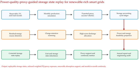
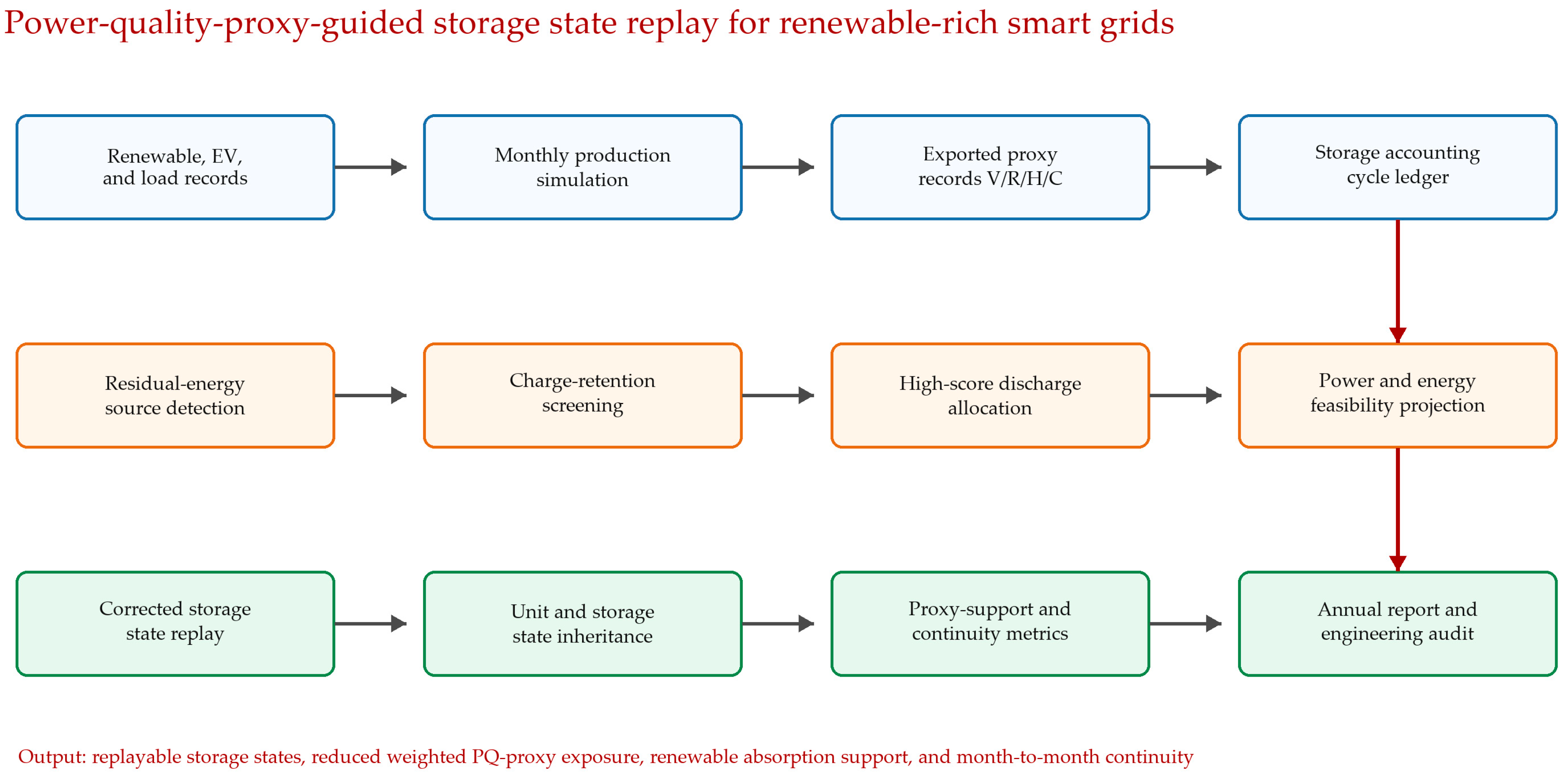
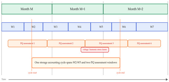
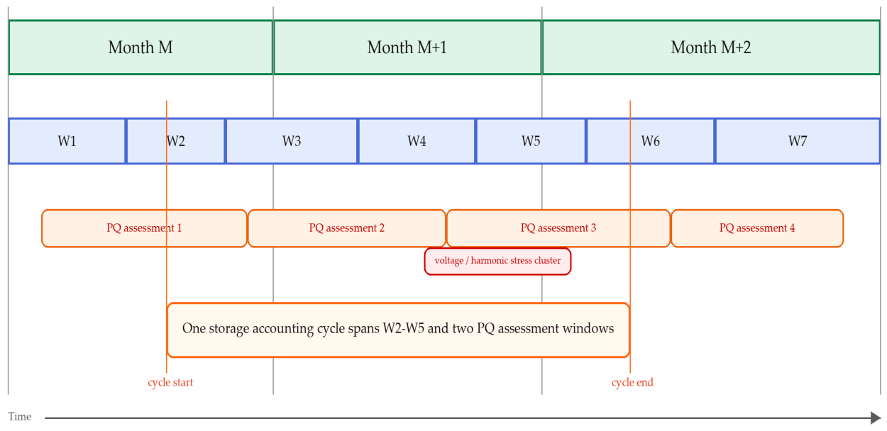
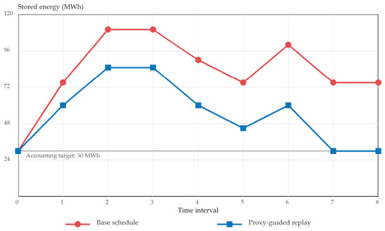
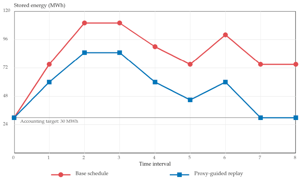
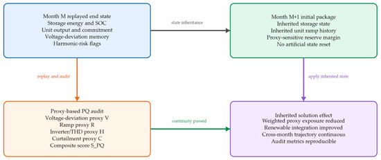
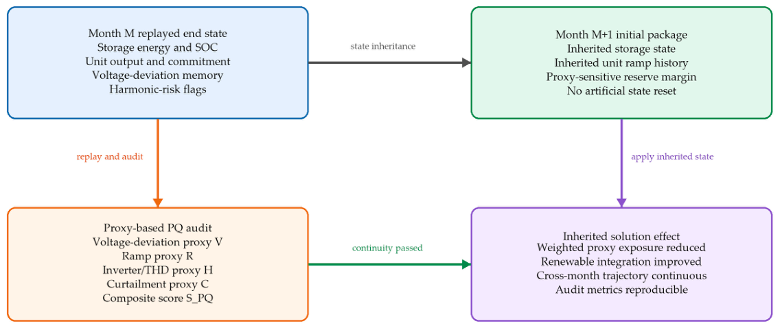

Disclaimer/Publisher’s Note: The statements, opinions and data contained in all publications are solely those of the individual author(s) and contributor(s) and not of MDPI and/or the editor(s). MDPI and/or the editor(s) disclaim responsibility for any injury to people or property resulting from any ideas, methods, instructions or products referred to in the content. |
© 2026 by the authors. Licensee MDPI, Basel, Switzerland. This article is an open access article distributed under the terms and conditions of the Creative Commons Attribution (CC BY) license.