Frequency-Adaptive Current Control with Kalman Filter-Based Observer for Multiple Grid-Connected Inverters Under Harsh Grid Distortion

Abstract

As renewable energy source-based distributed generation is more widely connected to the grid, stable current control and power quality improvement in grid-connected inverters (GCIs) become more important. To satisfy increasing power demand, multi-inverter systems connected to the grid in parallel are being widely adopted. However, parallel operation may degrade current quality and stability because of inverter interactions under harsh grid conditions. In particular, grid voltage harmonics, voltage imbalance, and frequency variations can also impair current control performance and system stability. To address these concerns, a frequency-adaptive current controller integrated with a Kalman filter (KF)-based observer is developed to ensure a stable operation of multiple GCIs. Moreover, a stability evaluation is presented for multi-inverter systems by using admittance-based stability analysis. A Kalman filter-based state observer is applied to improve the estimation accuracy under noisy measurement conditions. In addition, a moving average filter-based phase-locked loop (MAF-PLL) is applied to improve the detection accuracy and reliability of the grid frequency and phase angle under harsh grid conditions to ensure an effective frequency-adaptive control design. The effectiveness and performance of the proposed current controller are assessed through the PSIM simulations. The simulation results show that the MAF-PLL reduces the maximum frequency fluctuation from $\pm$7 Hz to $\pm$1.1 Hz. In addition, the KF-based observer reduces the RMS estimation error to 0.0001 A. On the other hand, those values are 1.3 A with the conventional observer and 0.0003 A with the LQR-based observer, respectively. The practicality of the proposed scheme is also confirmed experimentally using 2 kW parallel multiple GCI prototype systems under harsh grid conditions.

1. Introduction

Environmental concerns associated with conventional power systems have increased the importance of carbon reduction. As the deployment of renewable energy-based distributed generation (RE-DG), which supports low-carbon and economical energy supply, is expanded [1], the importance of ensuring stable power delivery through grid-connected inverters (GCIs) is increasing. Accordingly, multi-inverter systems operating in parallel with the grid are being more widely adopted to meet growing power demand. Such a parallel-connected structure is advantageous for expanding system capacity and flexibly accommodating distributed generation in the grid, but it is also structurally more sensitive to inverter coupling and variations in grid conditions. In parallel-connected GCI systems, maintaining reliable operation while achieving high efficiency and good power quality under harsh grid conditions, including harmonic distortion and voltage imbalance, becomes an important requirement [2]. In addition, GCI control techniques should conform to the power-quality criteria defined in IEEE Std. 1547 [3] and should also address issues arising from recent grid regulations and grid-code requirements [4].

GCI systems generally adopt pulse width modulation (PWM) switching control, which generates switching ripple and high-frequency harmonic components that can degrade current quality. Although an inductive (L) filter can reduce harmonic components, sufficient attenuation typically requires a large inductance, which can lead to a bulky filter and increased losses. Accordingly, inductive-capacitance-inductive (LCL) filters have been extensively employed in recent years because they offer effective suppression of high frequency harmonics and enable filter size reduction. Nevertheless, the inherent resonance of an LCL filter requires additional damping methods in controller design to ensure the system stability. Moreover, controller gain selection and damping design around the resonance frequency significantly affect system performance [5,6,7,8,9]. For this reason, GCI systems employing an LCL filter require a particular control approach that preserves the advantages of the filter while suppressing resonance-induced performance degradation. To address this issue, state-space current control is employed because it can systematically account for the resonant characteristics of the system. In this approach, state-feedback is used to handle the resonant poles directly [10]. However, such a control structure requires access to all state variables, including the filter capacitor voltages and inductor currents [11]. Therefore, an observer that can reconstruct the full state under limited sensor conditions is essential [12,13].

In a GCI system that involves grid impedance, the PCC voltage and grid-side states can be included in the system model, thereby increasing the system order and yielding a more complex state-space representation than that of a single LCL filter-based GCI. In particular, when additional states that are not directly measurable, such as the grid inductance current, are considered, it is difficult to acquire all the state variables required for state-feedback control. Under such conditions, unmeasured states must be reconstructed from limited measurement signals, which makes the state estimation structure more critical [14,15]. Furthermore, since state-space current control relies on feedback formed from the estimated states, the accuracy and reliability of state estimation directly influence current tracking performance, harmonic suppression capability, and overall system stability. Therefore, a reliable observer structure that can provide the state information under grid impedance and harsh grid conditions is essential.

In the observer implementation, non-ideal factors such as current and voltage sensor noise, switching ripple, and parameter uncertainties may introduce state estimation errors. These errors easily propagate into the state-feedback input, thereby degrading current tracking performance and power quality. State estimation accuracy under noisy measurement conditions has been studied in [16,17]. In parallel-connected GCI systems, estimation errors in an individual unit can affect the inverter control input and current response. Furthermore, estimation errors also influence other inverter units and the overall system operation through inverter interactions [18,19]. Therefore, a reliable state estimation technique under noisy measurement conditions is necessary for state-space current control of GCI systems operating in parallel. For this reason, the observer should be designed to attenuate the effect of measurement noise and model uncertainty on the estimated states used for feedback control [20]. In this study, this requirement is addressed by adopting a Kalman filter (KF)-based observer design to improve the reliability of state estimation.

Grid frequency variation is among the main factors that degrade current regulation performance in grid-connected inverters [21,22]. Conventionally, power imbalance between generation and load, load fluctuations, and output variations of distributed generation can cause grid frequency deviation. Such deviation can affect the detection accuracy of the grid frequency and phase angle required for coordinate transformation [23]. Moreover, frequency and phase angle detection errors deteriorate harmonic compensation performance and increase distortion in the grid-side current. Therefore, accurate grid frequency detection is necessary for stable current control under frequency variation.

Under harsh grid voltage conditions, accurate detection of grid frequency and phase angle becomes especially critical because the accuracy of detection has a direct influence on current control. However, the conventional phase-locked loop (PLL) method suffers from degraded detection accuracy under such harsh grid conditions [24,25]. Grid voltage harmonics and imbalance can introduce oscillatory components into the detected frequency and phase angle, which may deteriorate the reliability of the frequency information used for frequency-adaptive control. Therefore, a detection method that provides reliable frequency and phase angle information despite harsh grid conditions is required. A moving average filter (MAF) has been incorporated into the PLL structure to improve the phase and frequency detection under distorted and unbalanced grid voltages [26]. In this study, MAF-PLL is adopted to attenuate the effects of grid voltage distortion and imbalance. The detected information is then used in the coordinate transformation and frequency-adaptive current controller to achieve a good reference current tracking and harmonic suppression performance even under grid frequency variation and harsh grid conditions in a multiple GCI system.

Even when the current controller provides a satisfactory performance for each inverter unit, the overall system response can be deteriorated in the configuration of parallel multiple GCIs due to the interactions among the inverters. In a parallel configuration, multiple inverters share a point of common coupling (PCC), and the output behavior and control performance of each inverter may be affected by the other inverter units connected in parallel to the same PCC under the grid impedance. Moreover, because of the interactions among the inverters, it is difficult to expect that the control performance designed with a single inverter will remain unchanged in parallel multiple GCI operation. In particular, this structural coupling can alter the LCL filter resonance characteristics depending on the operating conditions or amplify current distortion in specific frequency ranges, thereby degrading the multiple GCI system stability. Hence, the verification of current quality and stability for the control method under parallel operating conditions is required [27,28], because the current response verified for an individual GCI may not fully represent that of a parallel multiple GCI system, where the inverter output admittances interact through the common PCC and grid impedance [29]. Accordingly, the stability verification should include the interaction effects among parallel GCIs as well as the current control performance of each inverter.

The interaction issue in a parallel multi-inverter structure has been systematically analyzed from the perspective of admittance [30]. In grid-connected inverter systems, admittance-based analysis is commonly used to investigate a possible stability degradation resulting from interaction between the inverter and the grid [31]. For parallel multiple GCIs with grid impedance, resonance characteristics and distortion in the output currents associated with the mutual influence between individual inverters are investigated using an admittance-based approach [32]. Furthermore, an interaction-admittance model has been used to represent the coupling among parallel inverter units and to describe the stability characteristics of the multiple GCI system [33]. Based on this framework, the admittance-based evaluation examines the interaction between the output admittances of the parallel inverters and the grid admittance. Accordingly, the stability of the proposed current controller under multiple GCIs with grid impedance is evaluated using this admittance-based stability analysis. In addition to the observer-based control, frequency-adaptive operation, and impedance/admittance-based stability studies discussed above, recent intelligent/adaptive stability monitoring studies are also reported for grid-connected converters under parameter-varying grid conditions [34,35]. These studies investigate stability monitoring or stability prediction under grid impedance variation and LCL filter parameter perturbation to improve the stability margin through controller coefficient adjustment. However, these studies mainly focus on online stability monitoring, stability prediction, or adaptive tuning rather than an integrated frequency-adaptive current control structure for parallel GCIs under harsh grid distortion.

This study introduces a frequency-adaptive state-space current control scheme for a parallel multiple GCI system under harsh grid conditions. This scheme includes a state-feedback current controller that incorporates integral action and resonant controllers, an MAF-PLL, and a KF-based observer. The integral controller improves reference current tracking, while the resonant controller suppresses harmonic components caused by voltage imbalance and distortion. The MAF-PLL provides accurate grid phase angle and frequency information for coordinate transformation in the environment of severe voltage distortion, voltage imbalance, and grid frequency variation. The KF-based observer estimates the state variables required for state-feedback control under noisy measurement conditions. Admittance-based stability analysis is also adopted to evaluate the stability of the parallel multiple GCIs where the grid impedance interacts with the total output admittance of the parallel inverters. The proposed current controller is further evaluated by the simulation conducted with Powersim (PSIM) tool (version 9.1, Powersim, Rockville, MD, USA) to assess its robustness and performance. The practical applicability of the proposed current controller is also confirmed experimentally using 2 kW parallel multiple GCI prototype systems under harsh grid conditions. The comparison summarized in Table 1 shows that the previous studies have addressed important technical issues related to GCIs. However, most studies focused on a specific issue and did not present a complete control and stability verification framework for parallel GCIs under harsh grid conditions. In Table 1, the studies in the first column [11,12,13,14,15,16,17,20] consider the state reconstruction and feedback current control. The studies in the second column [21,22,26] consider grid frequency variation and frequency-adaptive operation. The studies in the third column [27,28,29,30,31,32,33] consider grid impedance, converter-grid interaction, harmonic deterioration, and parallel inverter stability. Finally, the studies in the fourth column [34,35] consider online identification, adaptive tuning, and stability margin improvement under parameter variation. The symbol “✓” indicates that the corresponding technical issue is explicitly considered in the representative study group, whereas “Partially” indicates that the issue is addressed only in a limited scope.

Table 1. Comparison with the previous studies.

	[11,12,13,14,15,16,17,20]	[21,22,26]	[27,28,29,30,31,32,33]	[34,35]	Proposed Method
State-feedback/observer design	✓	Partially	Partially	$\times$	✓
Frequency-adaptive current control	$\times$	✓	$\times$	$\times$	✓
Harmonic frequency compensation	$\times$	Partially	Partially	$\times$	✓
Grid impedance	$\times$	$\times$	✓	✓	✓
Parallel inverter interaction	$\times$	$\times$	✓	$\times$	✓
Online identification/adaptive tuning	$\times$	$\times$	$\times$	✓	$\times$
Experimental validation	✓	✓	✓	✓	✓

Table 1 clarifies that the technical contribution of this study is not confined to the development of a new standalone PLL, observer, LQR controller, resonant controller, or admittance analysis method. Rather, the contribution lies in the coordinated design and verification of frequency-adaptive current control, KF-based observation, harmonic compensation, and admittance-based stability assessment for parallel GCIs under grid voltage distortion, voltage imbalance, grid frequency variation, noisy measurement conditions, and LC grid impedance. Therefore, the proposed method is positioned as an integrated current control and stability verification framework for parallel GCIs under harsh grid conditions.

The contributions of the proposed study are described as follows:

(i)

A current control design for frequency adaptation is formulated for parallel GCIs under grid voltage distortion, voltage imbalance, and grid frequency variation. By incorporating the grid frequency detected by the MAF-PLL into the state-feedback law, the controller maintains an accurate reference current tracking and harmonic compensation capability even under harsh grid conditions.

(ii)

A KF-based observer is employed to effectively estimate the state variables used for current control in parallel multiple GCIs under noisy measurement conditions. The KF-based observer significantly mitigates the effect of measurement noise on the estimated states and provides reliable state estimates for the state-feedback current controller. This estimation reliability also supports a stable operation in parallel multiple GCI systems.

(iii)

The proposed control scheme is verified through admittance-based stability analysis, PSIM simulations, and hardware experiments for a parallel multiple GCI system under harsh grid conditions. The results confirm a stable parallel operation, good reference current tracking, effective harmonic suppression, and reliable multiple GCI operation under voltage imbalance, harmonic voltage distortion, grid impedance, and grid frequency deviation.

2. System Model

2.1. State-Space Modeling of LCL-Filtered GCI with Grid Impedance

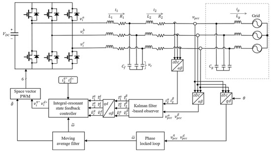
Figure 1 shows an LCL-filtered GCI, where the utility grid includes an LC grid impedance. In this study, voltage imbalance, harmonic distortion, and grid frequency variation are accounted for in the grid condition, and multiple GCIs are connected in parallel to a common PCC. The LCL filter comprises $L_1$, $L_2$, and $C_f$, whereas $L_g$ and $C_g$ represent the grid impedance. The variables $i_1$, $i_2$, and $v_c$ indicate the inverter-side currents, grid-side currents, and capacitor voltages, respectively. In Figure 1, $V_{dc}$, $v_i$, and $v_{pcc}$ indicate the DC-link voltage, inverter voltage, and PCC voltage, respectively. Likewise, $i_g$ and $V_g$ denote the grid inductance current and grid voltage, respectively. The superscripts $abc$, $\alpha \beta$, and $dq$ denote variables of the three-phase stationary frame, the stationary reference frame, and the synchronous reference frame (SRF), respectively.

Figure 1. Structure of the proposed current control method incorporating frequency adaptation and a Kalman filter-based observer.

In the proposed control structure, two PCC voltages and grid-side currents serve as measured variables, which are converted into the SRF for control realization. To detect the grid frequency $\tilde{\omega }$ and phase angle $\tilde{\theta }$, the PCC voltages are applied to the MAF-PLL. The detected information is then used in the coordinate transformation and the space vector PWM (SVPWM) generation. In addition, the measured signals are also provided to the KF-based observer to estimate the state variables for state-feedback control. The current controller with integral and resonant state-feedback produces the inverter voltage reference. The generated voltage reference is applied to the SVPWM along with the detected phase angle $\tilde{\theta }$ to produce the switching signals. In Figure 1, “~” and “$\ast$” denote a value detected by the MAF-PLL and a reference value, respectively.

The single GCI with the LC grid impedance is described in the SRF as [15]

$$\dot{\mathbf{x}}\left(t\right)=\mathbf{A}\mathbf{x}\left(t\right)+\mathbf{B}\mathbf{u}\left(t\right)+\mathbf{E}\mathbf{e}\left(t\right)$$

(1)

$$\mathit{y}\left(t\right)=\mathbf{C}\mathbf{x}\left(t\right)$$

(2)

where $\mathbf{x}={\left[i_2^q,i_2^d,i_1^q,i_1^d,v_c^q,v_c^d,v_{pcc}^q,v_{pcc}^d,i_g^q,i_g^d\right]}^T$ denotes the system state, $\mathbf{u}={\left[v_i^q,v_i^d\right]}^T$ denotes the system input, $\mathbf{e}={\left[v_g^q,v_g^d\right]}^T$ denotes the grid voltage, and $\mathbf{y}={\left[i_2^q,i_2^d\right]}^T$ denotes the system output. The corresponding matrices $\mathbf{A}$, $\mathbf{B}$, $\mathbf{C}$, and $\mathbf{E}$ are given by

$$\mathbf{A}=\left[\begin{array}{cccccccccc}0& -\omega & 0& 0& 1/L_2& 0& -1/L_2& 0& 0& 0\\ \omega & 0& 0& 0& 0& 1/L_2& 0& -1/L_2& 0& 0\\ 0& 0& 0& -\omega & -1/L_1& 0& 0& 0& 0& 0\\ 0& 0& \omega & 0& 0& -1/L_1& 0& 0& 0& 0\\ -1/C_f& 0& 1/C_f& 0& 0& -\omega & 0& 0& 0& 0\\ 0& -1/C_f& 0& 1/C_f& \omega & 0& 0& 0& 0& 0\\ 1/C_g& 0& 0& 0& 0& 0& 0& -\omega & -1/C_g& 0\\ 0& 1/C_g& 0& 0& 0& 0& \omega & 0& 0& -1/C_g\\ 0& 0& 0& 0& 0& 0& 1/L_g& 0& 0& -\omega \\ 0& 0& 0& 0& 0& 0& 0& 1/L_g& \omega & 0\end{array}\right]$$

(3)

$$\mathbf{B}=\left[\begin{array}{cc}0& 0\\ 0& 0\\ 1/L_1& 0\\ 0& 1/L_1\\ 0& 0\\ 0& 0\\ 0& 0\\ 0& 0\\ 0& 0\\ 0& 0\end{array}\right],\hspace{1em}\hspace{1em}\mathbf{E}=\left[\begin{array}{cc}0& 0\\ 0& 0\\ 0& 0\\ 0& 0\\ 0& 0\\ 0& 0\\ 0& 0\\ 0& 0\\ -1/L_g& 0\\ 0& -1/L_g\end{array}\right],\hspace{1em}\hspace{1em}\mathbf{C}=\left[\begin{array}{cccccccccc}1& 0& 0& 0& 0& 0& 0& 0& 0& 0\\ 0& 1& 0& 0& 0& 0& 0& 0& 0& 0\end{array}\right].$$

(4)

2.2. Discrete-Time Model with Digital Control Delay

To design a current controller, the models in (1) and (2) are converted into discrete- time form. In digital control systems, control inputs are updated at each sampling period. In addition, because of the computation and PWM update processes, the control input can be applied with a one-sampling period delay, which is incorporated into the system model [36]. Considering this effect, the corresponding discrete-time model is expressed as

$$\mathbf{x}(k+1)={\mathbf{A}}_d\mathbf{x}\left(k\right)+{\mathbf{B}}_d{\mathbf{u}}_d\left(k\right)+{\mathbf{E}}_d\mathbf{e}\left(k\right)$$

(5)

$${\mathbf{u}}_d\left(k+1\right)=\mathbf{u}\left(k\right)$$

(6)

$$\mathbf{y}\left(k\right)={\mathbf{C}}_d\mathbf{x}\left(k\right)$$

(7)

where ${\mathbf{u}}_d$ denotes the one-step delayed input. The matrices ${\mathbf{A}}_d$, ${\mathbf{B}}_d$, ${\mathbf{C}}_d$, and ${\mathbf{E}}_d$ denote the discretized system matrices for the sampling period $T_s$, and are given as [37]

$${\mathbf{A}}_d={\mathrm{e}}^{\mathbf{A}{T}_{\mathrm{s}}}, {\mathbf{B}}_d={\int }_0^{T_s}{e}^{\mathbf{A}\tau }\mathbf{B}d\tau , {\mathbf{C}}_d=\mathbf{C}, {\mathbf{E}}_d={\int }_0^{T_s}{e}^{\mathbf{A}\tau }\mathbf{E}d\tau .$$

(8)

3. Proposed Current Control Under Harsh Grid

In this section, a state-feedback current controller incorporating integral and resonant terms is designed to achieve accurate reference current tracking and harmonic compensation. In addition, the state variables are estimated using a KF-based observer, and the estimated states are supplied to the current controller. In particular, the KF-based observer enhances the reliability of state estimation despite measurement noise and parameter variations, thereby improving the effectiveness of the state-feedback control. Furthermore, the MAF-PLL provides reliable detection of the grid phase angle and frequency, supporting stable controller operation under grid voltage distortion and imbalance.

3.1. Frequency Detection Under Unbalanced and Distorted Grid

Distortion, imbalance, and frequency variation in the grid voltages can cause fluctuations in the frequency and phase angle detected by the PLL, and direct use of this information may degrade current control performance. Therefore, the MAF-PLL is employed to ensure reliable grid frequency estimation under harsh grid conditions. Figure 2 illustrates the MAF-PLL procedure used in [25,38]. In this structure, the PLL extracts the grid frequency and phase angle from the PCC voltages. The MAF suppresses the detected frequency fluctuations caused by harmonic distortion and noise. In particular, the window length of the MAF affects both the filtering effect and the transient frequency tracking response. A shorter window length reduces the filtering effect and results in larger frequency fluctuations under distorted grid voltages. An excessively long window length increases the delay and slows the transient frequency tracking response. In this study, the MAF window length is set to 90 samples to attenuate the frequency fluctuations caused by grid voltage distortion and retain acceptable transient frequency tracking performance. The resulting frequency is then used in the frequency-adaptive current controller to mitigate performance degradation under grid frequency variations.

Figure 2. Schematic of MAF-PLL for frequency and phase angle detection under harsh grid conditions.

3.2. Current Control Scheme Under LC Grid Impedance

To achieve reference current tracking and harmonic compensation, the state-feedback control includes integral and resonant states in the discrete-time system. The integral state reduces the steady-state error between the reference current and the sensed grid-side current, whereas the resonant states are incorporated to suppress selected harmonic components. The second-order resonant state is used for the harmonic suppression associated with grid voltage imbalance. In addition, the sixth- and twelfth-order resonant states are considered for the suppression of harmonic components associated with grid voltage distortion. The corresponding state dynamics are represented as

$${\mathbf{x}}_c\left(k+1\right)=\mathbf{G}{\mathbf{x}}_c\left(k\right)+\mathbf{H} \mathsf{\epsilon }\left(k\right)$$

(9)

where ${\mathbf{x}}_c={\left[\begin{array}{cccc}{\mathbf{x}}_I^T& {\mathbf{x}}_2^T& {\mathbf{x}}_6^T& {\mathbf{x}}_{12}^T\end{array}\right]}^T$ denotes the state variables of the integral and resonant terms, $\mathsf{\epsilon }={\left[\begin{array}{cc}{\epsilon }^q\left(k\right)& {\epsilon }^d\left(k\right)\end{array}\right]}^T={\mathbf{i}}_2^{\ast }-{\mathbf{C}}_d\mathbf{x}$ denotes the current error, and ${\mathbf{i}}_2^{\ast }={\left[\begin{array}{cc}{i}_2^{q\ast }& i_2^{d\ast }\end{array}\right]}^T$ denotes the reference current. The state ${\mathbf{x}}_I$ denotes the integral state, while ${\mathbf{x}}_2$, ${\mathbf{x}}_6$, and ${\mathbf{x}}_{12}$ denote the resonant states corresponding to the second-, sixth-, and twelfth-order harmonic components, respectively. The matrices $\mathbf{G}$ and $\mathbf{H}$ are defined as

$$\mathbf{G}=\left[\begin{array}{cccc}{\mathbf{A}}_i& & & \\ & {\mathbf{A}}_{r2}& & \\ & & {\mathbf{A}}_{r6}& \\ & & & {\mathbf{A}}_{r12}\end{array}\right], \mathbf{H}=T_{\mathrm{s}}\left[\begin{array}{c}{\mathbf{B}}_i\\ {\mathbf{B}}_{r2}\\ {\mathbf{B}}_{r6}\\ {\mathbf{B}}_{r12}\end{array}\right]$$

(10)

The matrices ${\mathbf{A}}_i$ and ${\mathbf{B}}_i$ denote the integral state dynamics, and ${\mathbf{A}}_{rj}$ and ${\mathbf{B}}_{rj}$ denote the resonant state dynamics for $j=2, 6, 12$. By incorporating (9) into (5) and (6), the entire system is formulated as

$$\left[\begin{array}{c}\mathbf{x}(k+1)\\ {\mathbf{u}}_d\left(k+1\right)\\ {\mathbf{x}}_c\left(k+1\right)\end{array}\right]=\left[\begin{array}{ccc}{\mathbf{A}}_d& {\mathbf{B}}_d& \mathbf{0}\\ \mathbf{0}& \mathbf{0}& \mathbf{0}\\ -\mathbf{H}{\mathbf{C}}_d& \mathbf{0}& \mathbf{G}\end{array}\right]\left[\begin{array}{c}\mathbf{x}\left(k\right)\\ {\mathbf{u}}_d\left(k\right)\\ {\mathbf{x}}_c\left(k\right)\end{array}\right]+\left[\begin{array}{c}\mathbf{0}\\ \mathbf{I}\\ \mathbf{0}\end{array}\right] \mathbf{u}\left(k\right)+\left[\begin{array}{c}{\mathbf{E}}_d\\ \mathbf{0}\\ \mathbf{0}\end{array}\right] \mathbf{e}\left(k\right)+\left[\begin{array}{c}\mathbf{0}\\ \mathbf{0}\\ \mathbf{H}\end{array}\right] {\mathbf{i}}_2^{\ast }\left(k\right)$$

(11)

For this system, the corresponding state-feedback control law is represented as follows:

$$\mathbf{u}\left(k\right)=-\mathbf{K}{\mathbf{x}}_s\left(k\right)=-\left[\begin{array}{ccc}{\mathbf{K}}_x& {\mathbf{K}}_u& {\mathbf{K}}_c\end{array}\right]\left[\begin{array}{c}\mathbf{x}\left(k\right)\\ {\mathbf{u}}_d\left(k\right)\\ {\mathbf{x}}_c\left(k\right)\end{array}\right]={\mathbf{u}}_x\left(k\right)+{\mathbf{u}}_u\left(k\right)+{\mathbf{u}}_c\left(k\right)$$

(12)

where ${\mathbf{x}}_s={\left[\begin{array}{ccc}{\mathbf{x}\left(k\right)}^T& {{\mathbf{u}}_d\left(k\right)}^T& {{\mathbf{x}}_c\left(k\right)}^T\end{array}\right]}^T$, ${\mathbf{u}}_x\left(k\right)=-{\mathbf{K}}_x\mathbf{x}\left(k\right)$, ${\mathbf{u}}_u\left(k\right)=-{\mathbf{K}}_u{\mathbf{u}}_d\left(k\right)$, ${\mathbf{u}}_c\left(k\right)=-{\mathbf{K}}_c{\mathbf{x}}_c\left(k\right)$, and $\mathbf{K}=\left[\begin{array}{ccc}{\mathbf{K}}_x& {\mathbf{K}}_u& {\mathbf{K}}_c\end{array}\right]$. The gains ${\mathbf{K}}_x$, ${\mathbf{K}}_u$, and ${\mathbf{K}}_c$ denote the gain matrices used in state-feedback control law for the plant states of the GCI, the one-sample delayed input caused by the digital control implementation, and the integral and resonant terms, respectively.

The optimal control gain $\mathbf{K}$ in (12) is derived through an LQR design approach in [39] with the performance index $\mathbf{J}$ defined for the augmented state-space model in (11) as follows:

$$\mathbf{J}={\displaystyle \frac{1}{2}}{\displaystyle \sum _{k=0}^{\infty }}{{\mathbf{x}}_s}^T\left(k\right)\mathbf{Q}{\mathbf{x}}_s\left(k\right)+{\mathbf{u}}^T\left(k\right)\mathbf{R}\mathbf{u}\left(k\right)$$

(13)

where $\mathbf{Q}$ is a positive semi-definite matrix, and $\mathbf{R}$ is a positive definite matrix. The state-feedback gain $\mathbf{K}$ is derived from the solution of the Algebraic Riccati Equation (ARE) related to the weighting matrices $\mathbf{Q}$ and $\mathbf{R}$. The weighting matrices significantly influence the system response including the reference current tracking performance, harmonic compensation characteristics, and the magnitude of the control input. In other words, the weighting matrices determine how strongly the tracking error, harmonic components, and control input magnitude are reflected in the LQR cost function. Therefore, the variation of the weighting coefficients changes the resulting feedback gain, which may alter the reference current tracking, harmonic suppression performance, and required control input magnitude. The optimal gain $\mathbf{K}$ is computed with the “dlqr” function to solve the corresponding ARE in MATLAB 2024a software. The matrices $\mathbf{Q}$ and $\mathbf{R}$ are selected as follows:

$$\mathbf{Q}=\left[\begin{array}{cccc}{\mathbf{I}}_{10\times 10}& {\mathbf{0}}_{10\times 2}& {\mathbf{0}}_{10\times 2}& {\mathbf{0}}_{10\times 12}\\ {\mathbf{0}}_{2\times 2}& {\mathbf{I}}_{2\times 2}& {\mathbf{0}}_{2\times 2}& {\mathbf{0}}_{2\times 12}\\ {\mathbf{0}}_{2\times 2}& {\mathbf{0}}_{2\times 2}& 6.3·{10}^8·{\mathbf{I}}_{2\times 2}& {\mathbf{0}}_{2\times 2}\\ {\mathbf{0}}_{12\times 2}& {\mathbf{0}}_{12\times 2}& {\mathbf{0}}_{12\times 2}& 0.021·{\mathbf{I}}_{12\times 12}\end{array}\right], \mathbf{R}=\left[\begin{array}{cc}1& 0\\ 0& 1\end{array}\right]$$

(14)

where the first term of $\mathbf{Q}$ corresponds to the plant states of the GCI system, the second term corresponds to the one-step delayed input, the third term corresponds to the integral states, and the fourth term corresponds to the resonant states. The large weighting coefficient assigned to the integral states is used to reduce the steady-state current tracking error, while the weight for the resonant states is used to improve harmonic compensation under distorted grid voltages. The matrix $\mathbf{R}$ is selected to limit the control input magnitude and prevent an excessive inverter voltage reference.

However, the resulting gain must be modified before it is applied to the state-feedback current controller since the grid inductance current is neither a measurable state nor an estimable state. Thus, the feedback gain corresponding to the grid inductance state should be excluded for state-feedback current controller. Therefore, the feedback gain should be restructured as

$$\mathbf{K}={\left[\begin{array}{cccc}{\mathbf{K}}_x^c& {\mathbf{0}}_{2\times 2}& {\mathbf{K}}_u& {\mathbf{K}}_c\end{array}\right]}_{2\times 26}$$

(15)

where ${\mathbf{K}}_x^c\in {\mathbb{R}}^{2\times 8}$ denotes the feedback gain for the measured and estimated state variables, and ${\mathbf{0}}_{2\times 2}$ denotes the zero matrix assigned to the uncertain states to exclude their effect. The matrices ${\mathbf{K}}_u\in {\mathbb{R}}^{2\times 2}$ and ${\mathbf{K}}_c\in {\mathbb{R}}^{2\times 14}$ are the feedback gains related to the delayed input, and the integral and resonant control.

3.3. Kalman Filter-Based Observer

A full-state current observer is applied to obtain the state variable information without requiring additional sensors. Although the LC grid impedance produces extra state variables to the GCI model, the grid-inductance current is difficult to measure or estimate directly. Therefore, the observer is constructed using the measurable grid-side current and PCC voltage to estimate the LCL filter states required for feedback control. In the multiple GCI system, measurement noise, switching ripple, and model uncertainty can affect the observer input and output signals, thereby reducing the accuracy and reliability of the estimated states. To overcome such limitations, a KF-based observer is employed.

When the grid frequency varies, an offline discretization cannot readily yield an accurate discrete-time model in the SRF because the GCI model is influenced by the grid frequency in the SRF. However, online discretization of the GCI model at every sampling period increases the computational demand for control implementation. To avoid the dependence on grid angular frequency in the observer model, the current observer is formulated in the stationary reference frame in this study. In the continuous-time, the GCI model is represented as follows:

$${\dot{\mathbf{x}}}_K\left(t\right)={\mathbf{A}}_{Kc}{\mathbf{x}}_K\left(t\right)+{\mathbf{B}}_{Kc}{\mathbf{u}}_K\left(t\right)+{\mathbf{E}}_{Kc}{\mathbf{e}}_K\left(t\right)$$

(16)

$${\mathbf{y}}_K\left(t\right)={\mathbf{C}}_{Kc}{\mathbf{x}}_K\left(t\right)$$

(17)

where ${\mathbf{x}}_K={\left[i_2^{\alpha },i_2^{\beta },i_1^{\alpha },i_1^{\beta },v_c^{\alpha },v_c^{\beta }\right]}^T$ is the system state, ${\mathbf{u}}_K={\left[v_i^{\alpha },v_i^{\beta }\right]}^T$ denotes the system input, ${\mathbf{e}}_K={\left[v_{pcc}^{\alpha },v_{pcc}^{\beta }\right]}^T$ denotes the PCC voltage, and ${\mathbf{y}}_K={\left[i_2^{\alpha },i_2^{\beta }\right]}^T$ denotes system output. The state-space matrices ${\mathbf{A}}_{Kc}$, ${\mathbf{B}}_{Kc}$, ${\mathbf{C}}_{Kc}$, and ${\mathbf{E}}_{Kc}$ are defined as follows:

$${\mathbf{A}}_{Kc}=\left[\begin{array}{cccccc}0& 0& 0& 0& 1/L_2& 0\\ 0& 0& 0& 0& 0& 1/L_2\\ 0& 0& 0& 0& -1/L_1& 0\\ 0& 0& 0& 0& 0& -1/L_1\\ -1/C_f& 0& 1/C_f& 0& 0& 0\\ 0& -1/C_f& 0& 1/C_f& 0& 0\end{array}\right],$$

(18)

$${\mathbf{B}}_{Kc}=\left[\begin{array}{cc}0& 0\\ 0& 0\\ 1/L_1& 0\\ 0& 1/L_1\\ 0& 0\\ 0& 0\end{array}\right],\hspace{1em}{\mathbf{E}}_{Kc}=\left[\begin{array}{cc}-1/L_2& 0\\ 0& -1/L_2\\ 0& 0\\ 0& 0\\ 0& 0\\ 0& 0\end{array}\right],\hspace{1em}{\mathbf{C}}_{Kc}=\left[\begin{array}{cccccc}1& 0& 0& 0& 0& 0\\ 0& 1& 0& 0& 0& 0\end{array}\right]$$

(19)

To facilitate digital implementation, the models in (15) and (16) are converted into a discrete-time form. In the GCI system, nonideal factors such as measurement noise, switching ripple, and model uncertainty may affect the observer estimation performance. Taking these factors into consideration, the discretized state-space model of (15) and (16) is expressed as

$${\mathbf{x}}_K\left(k+1\right)={\mathbf{A}}_{Kd}{\mathbf{x}}_K\left(k\right)+{\mathbf{B}}_{Kd}{\mathbf{u}}_K\left(k\right)+{\mathbf{E}}_{Kd}{\mathbf{e}}_K\left(k\right)+\mathsf{\omega }\left(k\right)$$

(20)

$${\mathbf{y}}_K\left(k\right)={\mathbf{C}}_{Kd}{\mathbf{x}}_K\left(k\right)+\mathsf{\upsilon }\left(k\right)$$

(21)

where ${\mathbf{A}}_{Kd}$, ${\mathbf{B}}_{Kd}$, ${\mathbf{C}}_{Kd}$, and ${\mathbf{E}}_{Kd}$ denote the discretized system matrices, $\mathsf{\omega }$ denotes process noise associated with model uncertainty and parameter variations, and $\mathsf{\upsilon }$ denotes measurement noise during output sensing, respectively. Then, the current observer is constructed as

$${\overline{\mathbf{x}}}_K(k+1)={\mathbf{A}}_{Kd}{\widehat{\mathbf{x}}}_K\left(k\right)+{\mathbf{B}}_{Kd}{\mathbf{u}}_K\left(k\right)+{\mathbf{E}}_K{\mathbf{e}}_K\left(k\right)$$

(22)

$${\widehat{\mathbf{x}}}_K(k+1)={\overline{\mathbf{x}}}_K\left(k+1\right)+{\mathbf{K}}_K\left({\mathit{y}}_K\left(k+1\right)-{\mathbf{C}}_{Kd}{\overline{\mathbf{x}}}_K(k+1)\right)$$

(23)

where ${\overline{\mathbf{x}}}_K$ denotes the predicted state vector based on the system dynamics and input signal, and ${\widehat{\mathbf{x}}}_K$ denotes the estimated state vector obtained by the predicted state and the output error correction term.

In KF-based current observer, the observer gain ${\mathbf{K}}_K$ in (22) is derived from the recursive calculation. In this study, the process noise covariance matrix ${\mathbf{Q}}_K$, the measurement noise covariance matrix ${\mathbf{R}}_K$, and the initial estimation error covariance matrix $\mathbf{P}\left(0\right)$ are selected as

$${\mathbf{Q}}_K=\mathrm{d}\mathrm{i}\mathrm{a}\mathrm{g}\left[\begin{array}{c}{10}^{-1}, {10}^{-1}, {10}^{-1},{10}^{-1},{10}^{-1},{10}^{-1}\end{array}\right],{\mathbf{R}}_K=\mathrm{d}\mathrm{i}\mathrm{a}\mathrm{g}\left[\begin{array}{c}1, 1\end{array}\right]$$

(24)

$$\mathbf{P}\left(0\right)=\mathrm{d}\mathrm{i}\mathrm{a}\mathrm{g}\left[\begin{array}{c}1, 1, 1, 1, 1, 1\end{array}\right].$$

(25)

The matrix ${\mathbf{Q}}_K$ reflects model uncertainty and parameter variations in the observer model, whereas ${\mathbf{R}}_K$ represents the noise level of the measured current and voltage signals. The initial covariance matrix $\mathbf{P}\left(0\right)$ represents the initial uncertainty of the estimated states before the recursive update starts. In the tuning procedure, ${\mathbf{R}}_K$ is first selected according to the measurement noise level of the sensed signals, and ${\mathbf{Q}}_K$ is then adjusted by checking the estimation error and the smoothness of the estimated state waveforms [40]. For this calculation, the prior estimation error covariance is determined as

$$\overline{\mathbf{P}}\left(k+1\right)={\mathbf{A}}_{Kd}\mathbf{P}\left(k\right){\mathbf{A}}_{Kd}^T+{\mathbf{Q}}_K$$

(26)

where $\overline{\mathbf{P}}$ and $\mathbf{P}$ denote the prior estimation error covariance and the posteriori estimation error covariance, respectively. The matrix ${\mathbf{Q}}_K$ denotes the covariance matrix of the process noise $\mathsf{\omega }$. Then, the observer gain ${\mathbf{K}}_K$ is determined as

$${\mathbf{K}}_K\left(k+1\right)=\overline{\mathbf{P}}\left(k+1\right){\mathbf{C}}_{Kd}^T{\left[{\mathbf{C}}_{Kd}\overline{\mathbf{P}}\left(k+1\right){\mathbf{C}}_{Kd}^T+{\mathbf{R}}_K\right]}^{-1}$$

(27)

where ${\mathbf{R}}_K$ denotes the covariance of the measurement noise $\mathsf{\upsilon }$. Then, the covariance of estimation error is updated as

$$\mathbf{P}\left(k+1\right)=\left(\mathbf{I}-{\mathbf{K}}_K\left(k+1\right){\mathbf{C}}_{Kd}\right)\overline{\mathbf{P}}\left(k+1\right).$$

(28)

The updated posteriori estimation error covariance is used in the recursive calculation for the KF-based observer. This recursive process reflects the influences of model uncertainty and measurement noise in the gain calculation and provides reliable state estimates for the proposed controller.

4. Stability Analysis

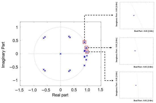
In this section, the designed control strategy is assessed from a stability perspective for the multiple GCI system. The eigenvalue analysis is conducted for the state matrix of the system in (11) with the restructured feedback gain in (15). Figure 3 presents the eigenvalues of the system in (11). As shown in Figure 3, all eigenvalues lie within the unit circle, which confirms the stability of the proposed control approach after the feedback gain restructuring. Moreover, the multiple GCI system is also analyzed by using a simplified equivalent circuit [32,41,42]. Since multiple GCIs share a common PCC, the current response of each inverter is affected not only by its own controller but also by the interactions among parallel inverters. Therefore, the overall system stability cannot be sufficiently explained by considering only the behavior of a single inverter. The interaction characteristics among the inverters and the effect of the grid voltage are examined to confirm overall system stability.

Figure 3. Eigenvalues of the proposed control scheme. The cross marks indicate the eigenvalue locations.

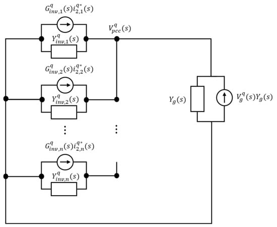
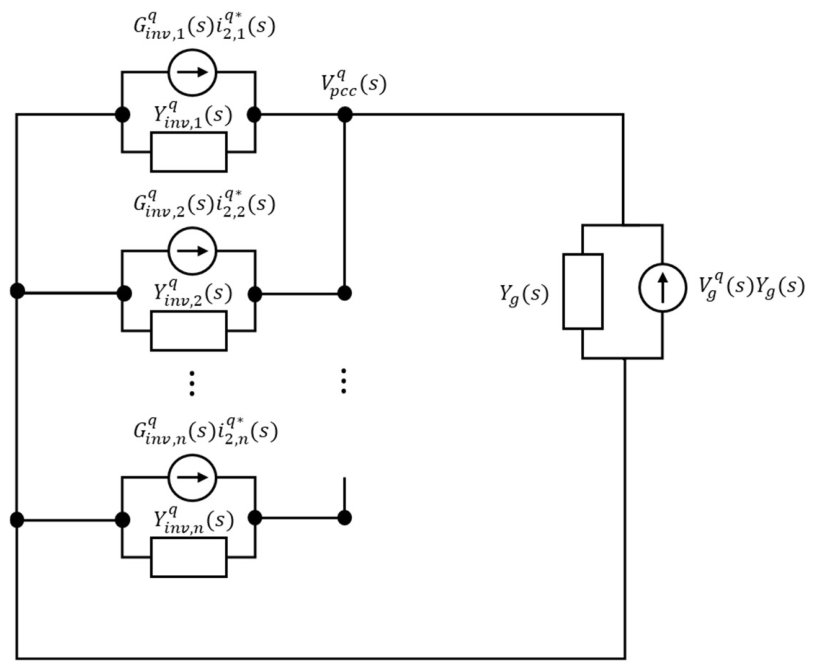
Figure 4 represents the Norton equivalent circuit for the multiple GCI system, which is used to assess the stability of the proposed scheme. From this equivalent circuit, $Y_{inv,m}\left(s\right)$, $G_{inv,m}\left(s\right)$, $Y_g\left(s\right)$, the grid-side current corresponding to the $m$-th inverter, and the PCC voltage can be obtained as

$$Y_{inv,m}^q\left(s\right)=-\left[\begin{array}{cc}1& 0\end{array}\right]\left[\begin{array}{cc}{\displaystyle \frac{i_{2,m}^q}{V_{pcc}^q}}& {\displaystyle \frac{i_{2,m}^q}{V_{pcc}^q}}\\ {\displaystyle \frac{i_{2,m}^d}{V_{pcc}^d}}& {\displaystyle \frac{i_{2,m}^d}{V_{pcc}^d}}\end{array}\right]\left[\begin{array}{c}1\\ 0\end{array}\right]$$

(29)

$$G_{inv,m}^q\left(s\right)=\left[\begin{array}{cc}1& 0\end{array}\right]\left[\begin{array}{cc}{\displaystyle \frac{i_{2,m}^q}{i_{2,m}^{q\ast }}}& {\displaystyle \frac{i_{2,m}^q}{i_{2,m}^{d\ast }}}\\ {\displaystyle \frac{i_{2,m}^d}{i_{2,m}^{q\ast }}}& {\displaystyle \frac{i_{2,m}^d}{i_{2,m}^{d\ast }}}\end{array}\right]\left[\begin{array}{c}1\\ 0\end{array}\right]$$

(30)

$$Y_g\left(s\right)=C_{g}s+{\displaystyle \frac{1}{L_{g}s}}={\displaystyle \frac{C_g{L}_g{s}^2+1}{L_{g}s}}$$

(31)

$$i_{2,m}^q=G_{inv,m}^q\left(s\right)i_{2,m}^{q\ast }-Y_{inv,m}^q\left(s\right)V_{pcc}^q\left(s\right)$$

(32)

$$V_{pcc}^q\left(s\right)={\displaystyle \frac{V_g^q\left(s\right)Y_g\left(s\right)+{\displaystyle {\sum }_{k=1}^n}{G}_{inv,k}^q\left(s\right)i_{2,k}^{q\ast }}{Y_g\left(s\right)+{\displaystyle {\sum }_{k=1}^n}{Y}_{inv,k}^q\left(s\right)}}.$$

(33)

where the subscript $m$ denotes the $m$-th inverter, $n$ denotes the number of inverters connected in parallel, $Y_{inv,m}^q$ denotes the inverter output admittance of $m$-th inverter, $G_{inv,m}^q$ denotes the closed-loop response of the inverter, and $Y_g$ denotes the grid admittance. For the $m$-th inverter, $i_{2,m}^q$, $i_{2,m}^{q\ast }$, and $V_{pcc}^q\left(s\right)$ represent the grid-side current, the reference current, and the PCC voltage, respectively.

Figure 4. Norton equivalent circuit for the multiple GCI system.

By substituting the PCC voltage (30) into (29), the grid-side current of the $m$-th inverter can be rewritten in terms of the reference current tracking component, the interaction component, and the grid voltage influence component as follows:

$$\begin{gathered} i_{2,m}^q\left(s\right)=\left(G_{inv,m}^q-{\displaystyle \frac{G_{inv,m}^q\left(s\right)Y_{inv,m}^q\left(s\right)}{Y_g\left(s\right)+{\displaystyle {\sum }_{k=1}^n}{Y}_{inv,k}^q\left(s\right)}}\right)i_{2,m}^{q\ast }\left(s\right)-{\displaystyle \frac{Y_m^q\left(s\right)\left({\displaystyle {\sum }_{l=1,l\ne m}^n}{G}_{inv,l}^q\left(s\right)i_{2,l}^{q\ast }\right)}{Y_g\left(s\right)+{\displaystyle {\sum }_{k=1}^n}{Y}_{inv,k}^q\left(s\right)}} \\ -{\displaystyle \frac{Y_{inv,m}^q\left(s\right)Y_g\left(s\right)}{Y_g\left(s\right)+{\displaystyle {\sum }_{k=1}^n}{Y}_{inv,k}^q\left(s\right)}}{V}_g^q\left(s\right) \end{gathered}$$

(34)

$$R_m\left(s\right)={\displaystyle \frac{i_{2,m}^q\left(s\right)}{i_{2,m}^{q\ast }\left(s\right)}}=G_{inv,m}^q-{\displaystyle \frac{G_{inv,m}^q\left(s\right)Y_{inv,m}^q\left(s\right)}{Y_g\left(s\right)+{\displaystyle {\sum }_{k=1}^n}{Y}_{inv,k}^q\left(s\right)}}$$

(35)

$$P_{m,l}\left(s\right)={\displaystyle \frac{i_{2,m}^q\left(s\right)}{i_{2,l}^{q\ast }\left(s\right)}}=-{\displaystyle \frac{Y_m^q\left(s\right)G_{inv,l}^q\left(s\right)}{Y_g\left(s\right)+{\displaystyle {\sum }_{k=1}^n}{Y}_{inv,k}^q\left(s\right)}}$$

(36)

$$M_G\left(s\right)={\displaystyle \frac{i_{2,m}^q\left(s\right)}{V_g^q\left(s\right)}}=-{\displaystyle \frac{Y_{inv,m}^q\left(s\right)Y_g\left(s\right)}{Y_g\left(s\right)+{\displaystyle {\sum }_{k=1}^n}{Y}_{inv,k}^q\left(s\right)}}.$$

(37)

where $R_m\left(s\right)$ indicates the reference current tracking characteristic of the $m$-th inverter, $P_{m,l}\left(s\right)$ indicates the interaction of $l$-th inverter on the $m$-th inverter, and $M_G\left(s\right)$ indicates how the grid voltage affects the current response in the $m$-th inverter. From these transfer functions, the multiple GCI system stability can be analyzed with the inverter output admittance and the grid admittance.

The stability of the proposed multiple GCI system is examined through $R_m\left(\mathrm{s}\right)$, $P_{m,l}\left(\mathrm{s}\right)$, and $M_G\left(\mathrm{s}\right)$. Since these transfer functions share a common denominator that is constituted by the grid admittance and the total output admittance of the parallel inverters, the corresponding phase difference should not approach ${180}^{\circ }$ at a frequency where the magnitudes of the two admittances become close to each other. Otherwise, the common denominator approaches zero, which significantly increases the magnitudes of $R_m\left(s\right)$, $P_{m,l}\left(s\right)$, and $M_G\left(s\right)$, and may yield unstable operation of the multiple GCI system. In addition, the magnitudes of $P_{m,l}\left(s\right)$ and $M_G\left(s\right)$ should remain below 0 dB to limit the effects of inverter interaction and grid voltage influence on the current response.

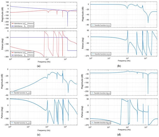
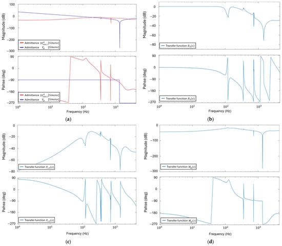
To support the admittance-based stability criterion, Figure 5 presents the Bode plots of the parallel GCI system. Figure 5a presents the Bode plots of the total inverter output admittance $2Y_{inv,1}^q(s)$ and the grid admittance $Y_g(s)$. The stability condition is examined by checking whether the common denominator of the admittance-based transfer functions approaches zero. The common denominator is expressed as $D\left(s\right)=Y_g\left(s\right)+2Y_{inv,1}^q\left(s\right).$ This critical condition can occur when $D\left(j\omega \right)$ approaches zero. At this critical condition, the magnitudes of $2Y_{inv,1}^q(j\omega )$ and $Y_g(j\omega )$ are equal, and their phase difference is ${180}^{\circ }$ at the same frequency.

Figure 5. Frequency responses when both inverter #1 and inverter #2 are in operation. (a) Magnitude and phase plots of 2$Y_{inv,1}^q$ and $Y_g\left(s\right)$; (b) magnitude and phase plots of $R_1$; (c) magnitude and phase plots of $P_{\mathrm{1,2}}$; (d) magnitude and phase plots of $M_G$.

In Figure 5a, four admittance intersection frequencies are observed at 406 Hz, 718 Hz, 745 Hz, and 2366 Hz. The corresponding phase differences are ${132}^{\circ }$, $-{32}^{\circ }$, ${108}^{\circ }$, and ${134}^{\circ }$, respectively. Accordingly, the phase stability margins are ${48}^{\circ }$, ${212}^{\circ }$, ${78}^{\circ }$, and ${46}^{\circ }$, respectively. Therefore, the common denominator of the transfer functions does not approach zero, which proves the stable operation of the multiple GCI systems.

Figure 5b–d further support the admittance-based stability assessment by presenting the frequency responses of $R_1\left(s\right)$, $P_{\mathrm{1,2}}\left(s\right)$, and $M_G\left(s\right)$, respectively. Figure 5b demonstrates a good reference current tracking characteristic of inverter #1 because the magnitude and phase of $R_1\left(s\right)$ remain close to 0 dB and $0^{\circ }$ in the low-frequency range. Figure 5c,d confirm that the interaction effect from inverter #2 and the grid voltage influence on inverter #1 are effectively attenuated because the magnitudes of $P_{\mathrm{1,2}}\left(s\right)$ and $M_G\left(s\right)$ remain below 0 dB over the entire frequency range. These results verify that the proposed controller ensures a stable operation of the parallel multiple GCI system under the grid impedance.

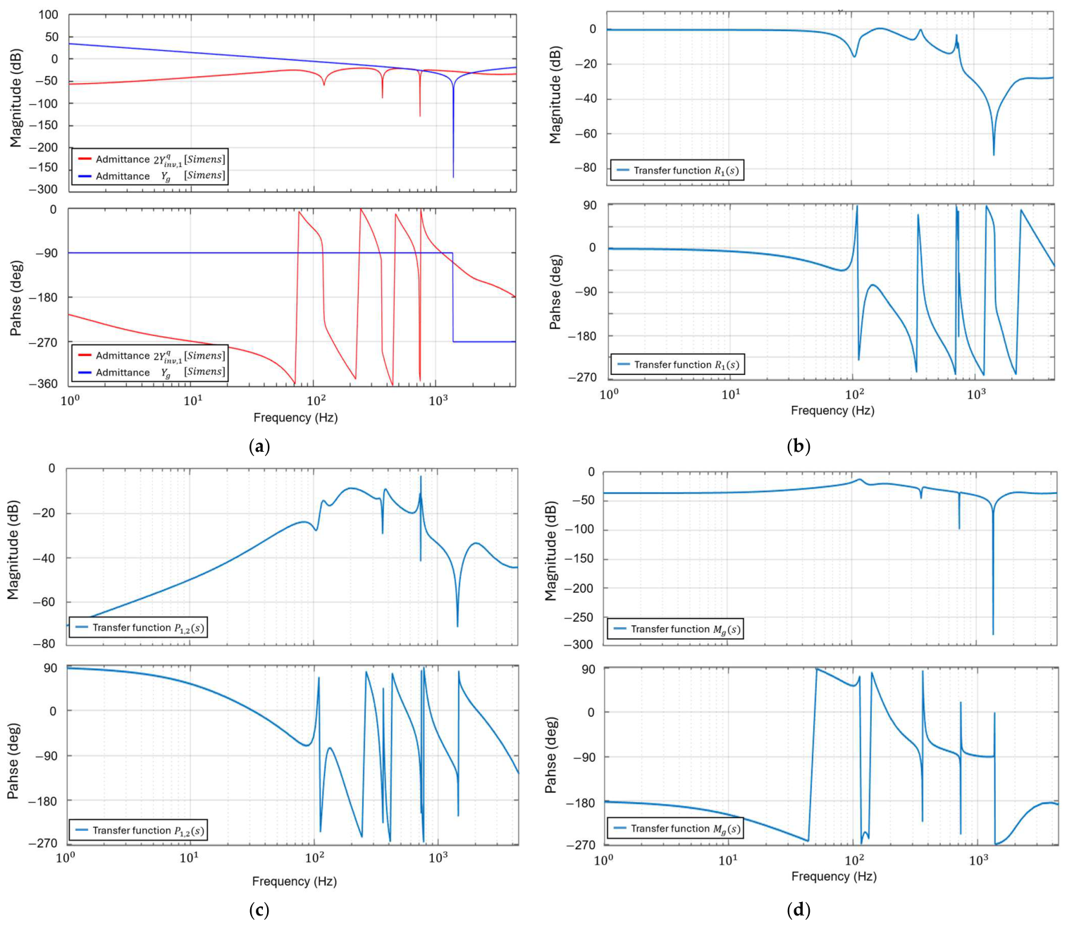
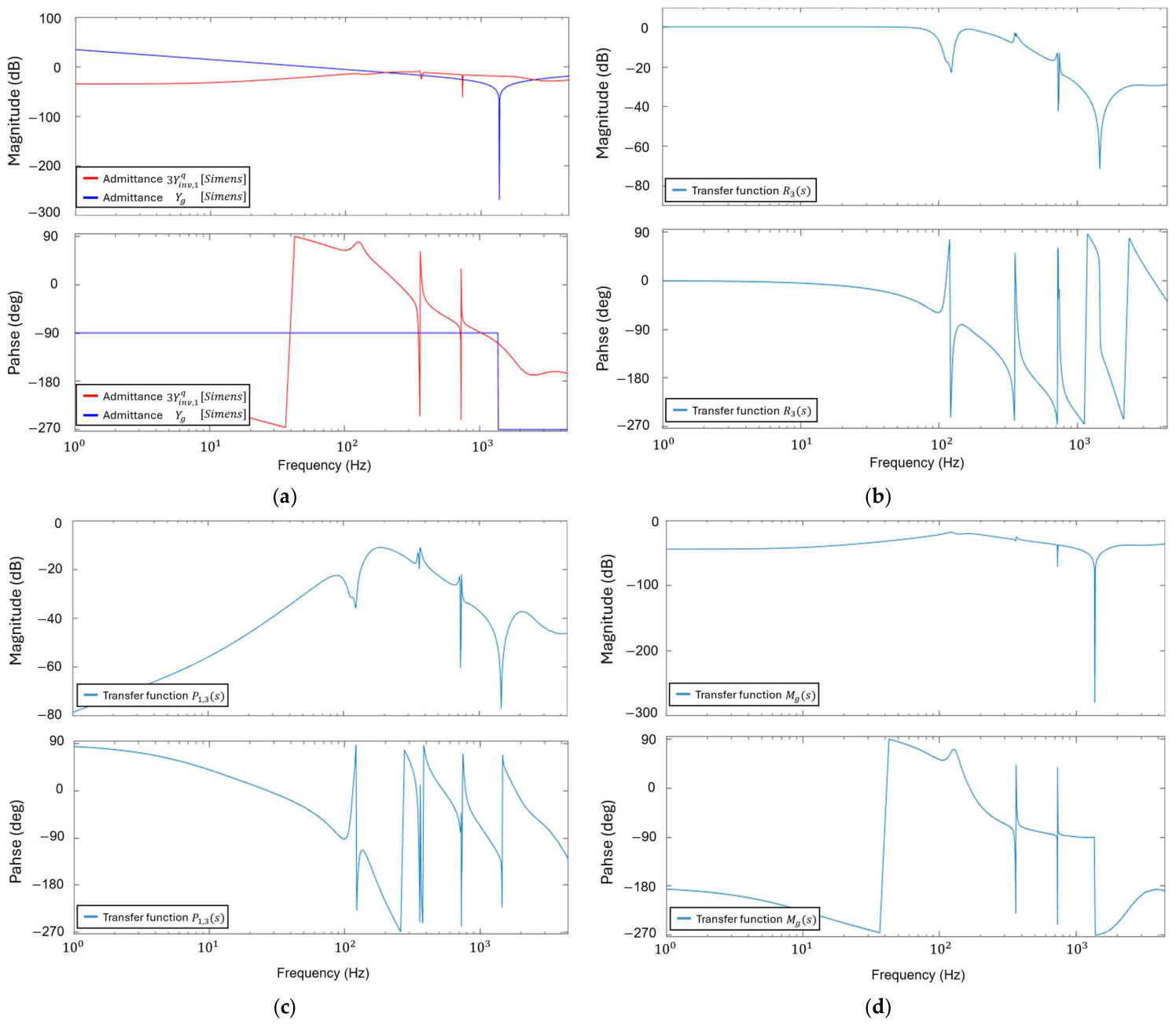
Figure 6 presents the frequency responses for $3Y_{inv,1}^q$, $Y_g\left(s\right)$, $R_3\left(s\right)$, $P_{\mathrm{1,3}}\left(s\right)$, and $M_G\left(s\right)$ in case of the three parallel GCIs. Figure 6a compares the total inverter admittance $3Y_{inv,1}^q(s)$ and the grid admittance $Y_g\left(s\right)$. Although their magnitudes intersect at several frequencies, the phase difference does not approach ${180}^{\circ }$, which confirms that the three parallel GCIs maintain stable operation. Figure 6b shows the magnitude and phase plots of $R_3\left(s\right)$, which represents the reference current tracking characteristic of inverter #3. The magnitude and phase remain close to 0 dB and $0^{\circ }$ in the low-frequency range, indicating that the inverter #3 tracks the reference current well when three parallel GCIs operate. Figure 6c shows the magnitude and phase plots of $P_{\mathrm{1,3}}\left(s\right)$, which represents the interaction effect of the inverter #3 on the current response of inverter #1. The magnitude remains below 0 dB over the entire frequency range, which demonstrates that the interaction effect from inverter #3 is attenuated. Figure 6d shows the magnitude and phase plots of $M_G\left(s\right)$, which represents the influence of the grid voltage on the current response. Similarly, the magnitude remains below 0 dB over the entire frequency range, which verifies that the grid voltage influence is sufficiently reduced. This analysis validates that the three parallel GCIs maintain stable operation under the LC grid impedance.

Figure 6. Frequency responses for three parallel GCIs. (a) Magnitude and phase plots of 3${\mathit{Y}}_{\mathit{i}\mathit{n}\mathit{v},\mathbf{1}}^{\mathit{q}}$ and ${\mathit{Y}}_{\mathit{g}}\left(\mathit{s}\right)$; (b) magnitude and phase plots of ${\mathit{R}}_{\mathbf{3}}$; (c) magnitude and phase plots of ${\mathit{P}}_{\mathbf{1},\mathbf{3}}$; (d) magnitude and phase plots of ${\mathit{M}}_{\mathit{G}}$.

5. Simulation Results

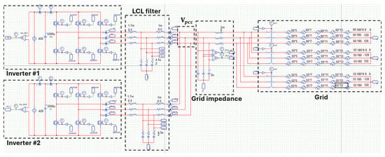
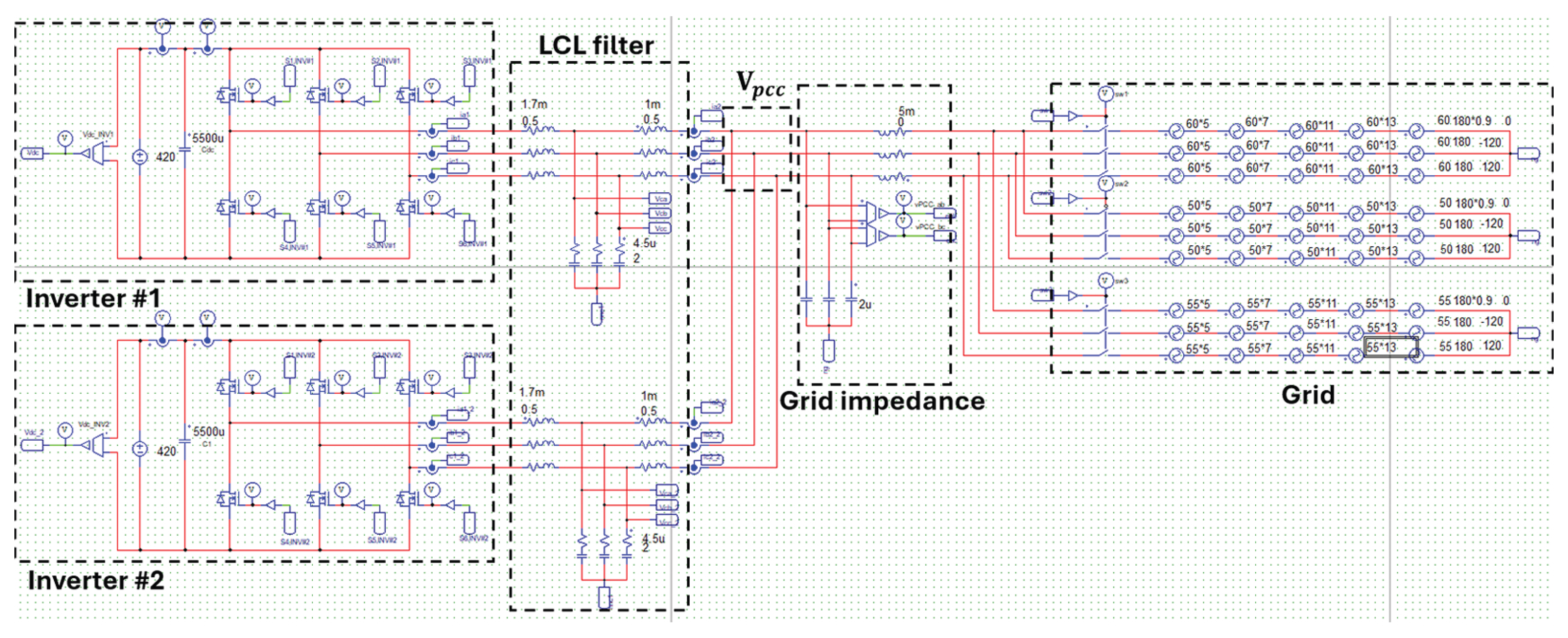
The designed current controller for multiple GCIs is evaluated through PSIM and MATLAB simulations under grid frequency variations, LC grid impedance, and harsh grid conditions. In the simulation, measurement noise is superimposed on the sensed current and voltage signals to emulate practical measurement conditions. The noise is set to 0.5% of the full-scale range of each sensing signal. Figure 7 presents the PSIM model for the multiple GCI system. The detailed parameter values in the PSIM schematic are shown in Table 2. In Table 2, for symbols with two subscripts, the second subscript denotes the number of the inverter.

Figure 7. PSIM schematic of the multiple GCI system.

Table 2. Parameters of a GCI system.

Parameters	Symbol	Value	Units
DC-link voltages	$V_{DC,1}$, $V_{DC,2}$	420	V
Grid-side filter inductances	$L_{2,1}$, $L_{2,2}$	1.0	mH
Inverter-side filter inductances	$L_{1,1}$, $L_{1,2}$	1.7	mH
Filter capacitances	$C_{f,1}$, $C_{f,2}$	4.5	µF
Grid voltage (line-to-neutral)	$V_g$	180	V
Grid frequency	f	60/50/55	Hz
Grid capacitance	$C_g$	4.5	µF
Grid inductance	$L_g$	3	mH
Switching frequency	$f_{sw}$	10	kHz
Sampling frequency	$f_s$	10	kHz

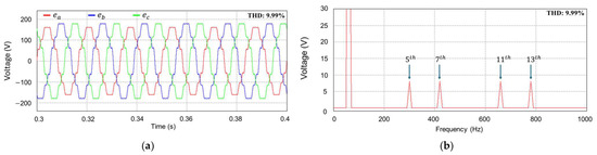
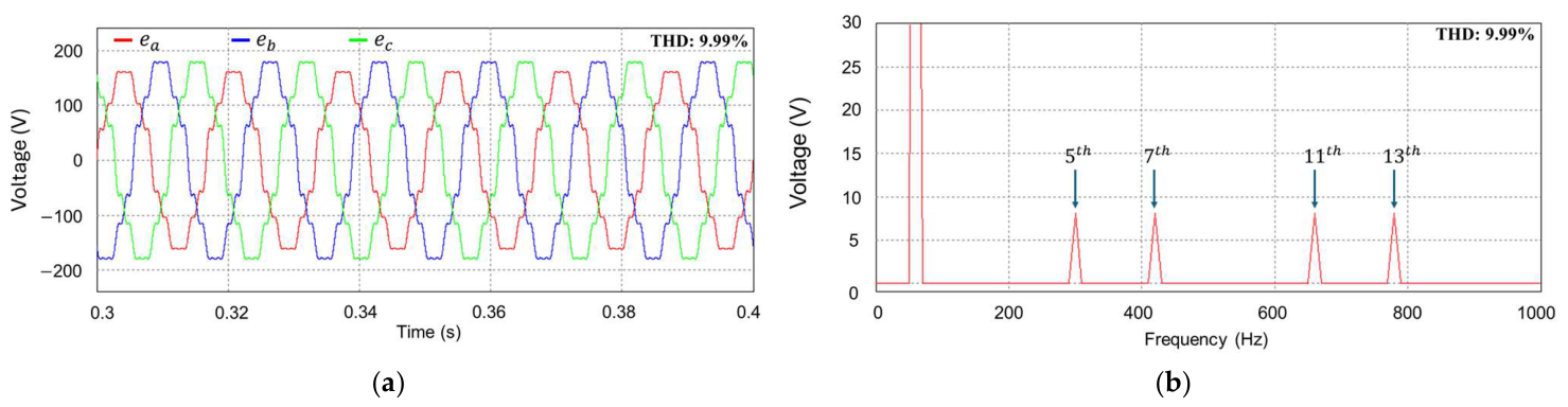
Figure 8a presents the distorted and unbalanced grid voltage waveforms, and Figure 8b shows the FFT result for the grid voltage in phase $a$. As shown in the figures, the grid voltage contains the fifth-, seventh-, eleventh-, and thirteenth-order harmonic components, each set to 5% of the nominal voltage. As a result, the grid voltage THD is 9.99%.

Figure 8. Grid voltages including distortion and imbalance. (a) Grid voltages; (b) FFT result for grid voltage in phase $a$.

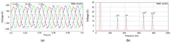
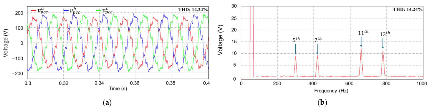
Figure 9a illustrates the PCC voltage waveforms under LC grid impedance and harsh grid voltages, and Figure 9b presents the FFT result for PCC voltage in phase $a$. The LC grid impedance and harsh grid voltages make the PCC voltage more distorted than the grid voltage. Consequently, the THD of the PCC voltage increases to 14.24%. These PCC voltage conditions are imposed in the simulation to verify the proposed control scheme.

Figure 9. PCC voltages under LC grid impedance and harsh grid condition. (a) PCC voltages; (b) FFT result for PCC voltage in phase $a$.

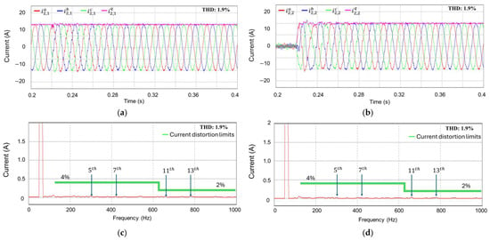
Figure 10a,b show the simulation results of the multiple GCIs under the previously defined grid conditions with the current controller proposed in this study. These figures present the three-phase grid-side current waveforms and $q$-axis current responses for inverter #1 and inverter #2, respectively. Until 0.23 s, only inverter #1 operates. Before 0.23 s, inverter #2 is connected in parallel to PCC without injecting currents. Only after 0.23 s, two inverters operate in parallel under the $q$-axis current reference of 10 A. It is confirmed that both inverters achieve accurate reference current tracking and operate stably in parallel. Also, the currents at the grid side retain sinusoidal waveforms. Figure 10c,d present the FFT results for the grid-side current in phase $a$ of inverter #1 and inverter #2 at the steady-state, respectively. The FFT results confirm that the harmonic components are effectively suppressed in both inverters, and the current THDs are 1.9% in both inverters, satisfying the current distortion limits specified in IEEE Std. 1547.

Figure 10. Simulation results of the current responses when both inverter #1 and inverter #2 are in operation. (a) Grid-side current responses of inverter #1; (b) grid-side current responses of inverter #2; (c) FFT result for grid-side current in phase $a$ of inverter #1; (d) FFT result for grid-side current in phase $a$ of inverter #2.

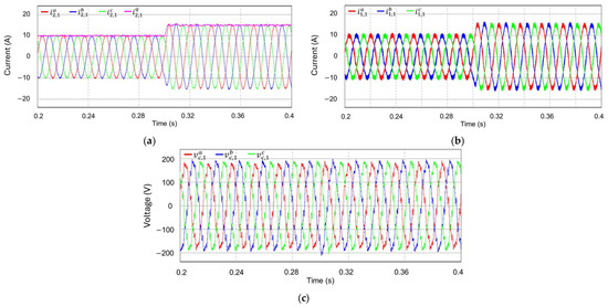
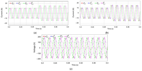
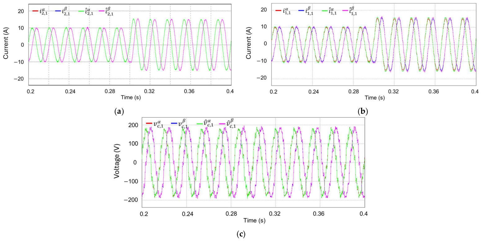
Figure 11 presents the transient performance of the parallel multiple GCI system under distorted and unbalanced PCC voltages with LC grid impedance when the reference current increases from 10 A to 15 A at 0.3 s. Figure 11a–c illustrate the grid-side and inverter-side currents together with the capacitor voltages, respectively. Figure 11 confirms that the proposed current controller achieves a fast transient response and maintains stable current without current distortion caused by parallel inverter interaction.

Figure 11. Simulation results of the transient performance for a step increase in the $q$-axis current reference of inverter #1 at 0.3 s when both inverter #1 and inverter #2 are in operation. (a) Grid-side current responses of inverter #1; (b) inverter-side current responses of inverter #1; (c) capacitor voltage responses of inverter #1.

Figure 12 shows the estimation results of the KF-based current observer. To prove the estimation performance, these figures compare the measured and estimated waveforms of inverter #1 when both inverter #1 and #2 are in operation. Figure 12a–c present the grid-side and inverter-side currents together with the capacitor voltages. Figure 12 clearly validates that the proposed observer provides accurate state estimation performance.

Figure 12. Measured and estimated waveforms of the current observer for a step increase in the $q$-axis current reference of inverter #1 at 0.3 s when both inverter #1 and inverter #2 are in operation. (a) Grid-side current estimation of inverter #1; (b) inverter-side current estimation of inverter #1; (c) capacitor voltage estimation of inverter #1.

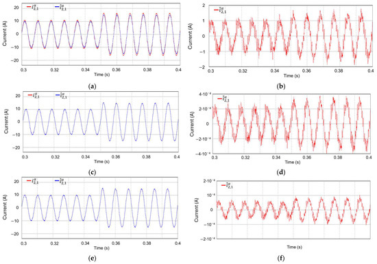
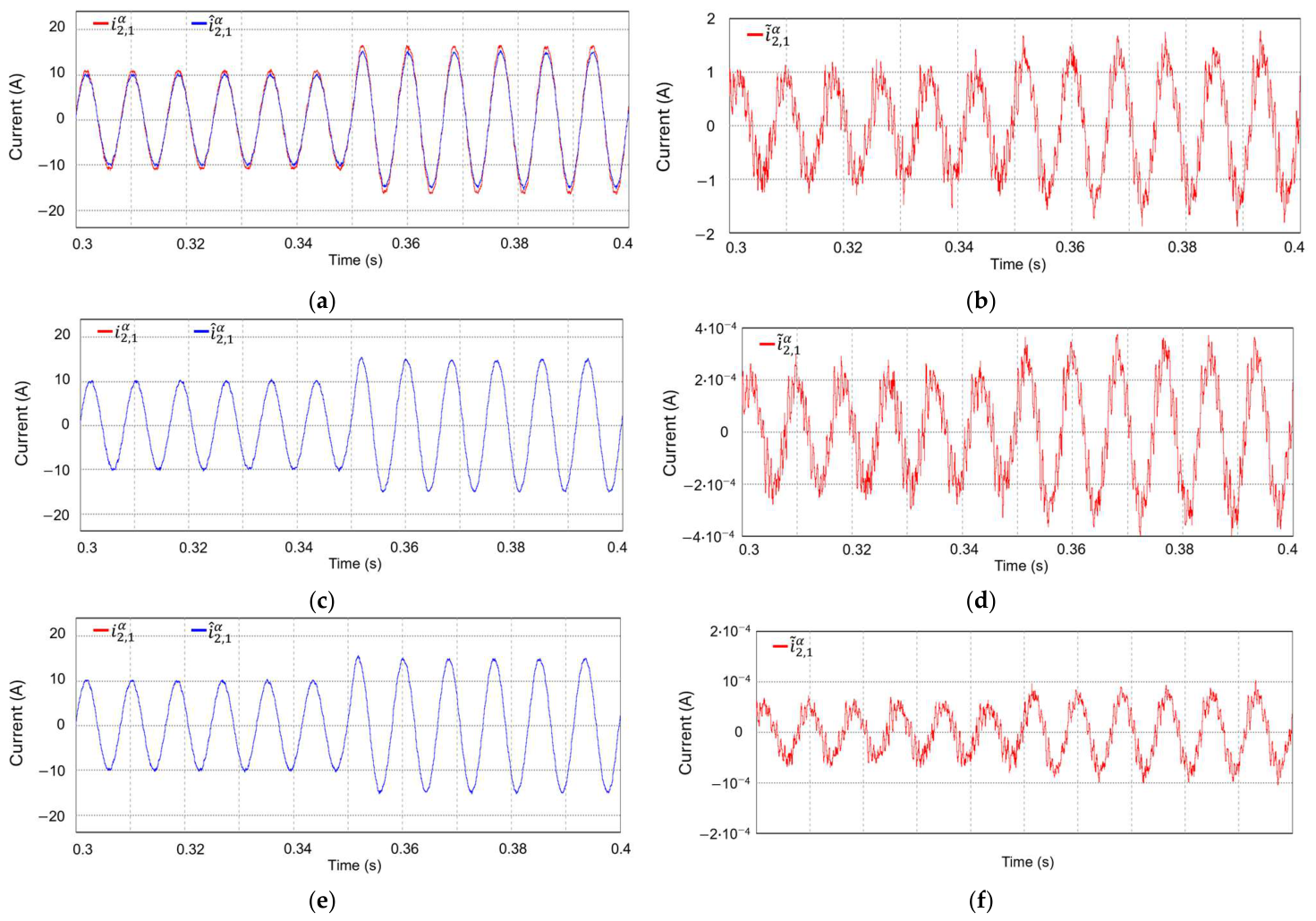
Figure 13 presents the comparison of the estimation performance for the conventional observer, LQR-based observer, and KF-based observer when the measurement noise is added to the sensed current and voltage. The Gaussian white noise corresponding to 0.5% magnitude of the full-scale sensing signal is applied in the sensor measurement. Figure 13a,c,e show the measured and estimated values for the conventional observer, LQR-based observer, and KF-based observer, respectively. Figure 13b,d,f show the estimation error between the measured and estimated values for each observer. Among the three observer design methods, the KF-based observer shows the smallest estimation error. These results verify that the proposed KF-based observer improves state estimation accuracy in the presence of noise.

Figure 13. Comparison of the estimation performance for different observers implemented in the stationary reference frame under noisy measurement conditions. (a) Measured and estimated values of the conventional observer; (b) estimation error of the conventional observer; (c) measured and estimated values of the LQR-based observer; (d) estimation error of the LQR-based observer; (e) measured and estimated values of the KF-based observer; (f) estimation error of the KF-based observer.

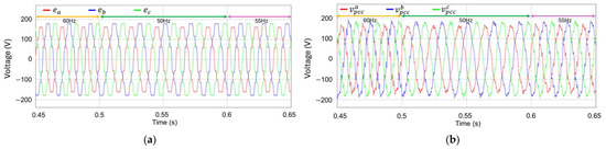
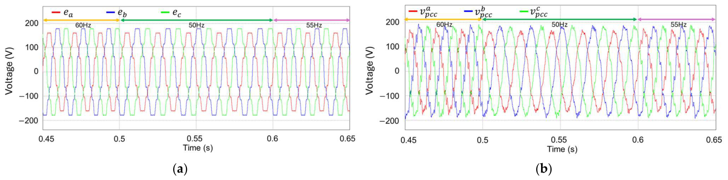
Figure 14 presents the grid voltage conditions applied to evaluate the proposed controller under grid frequency transition. Figure 14a presents the grid voltages with distortion and imbalance, where the grid frequency changes to 50 Hz and 55 Hz, at 0.5 s and 0.6 s, respectively. Figure 14b shows the corresponding PCC voltages.

Figure 14. Distorted and unbalanced grid and PCC voltages with grid frequency transitions at 0.5 s and 0.6 s. (a) Grid voltages; (b) PCC voltages.

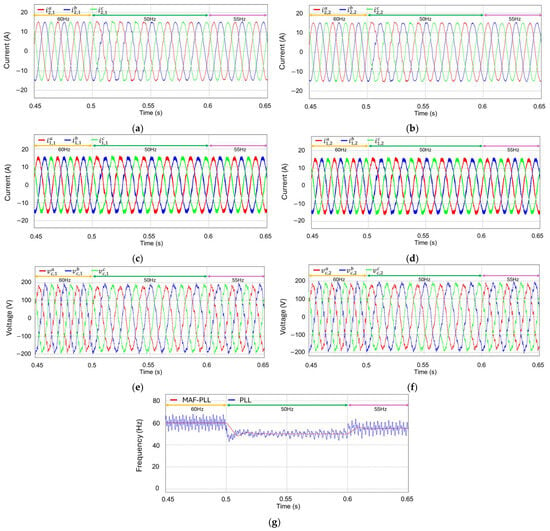
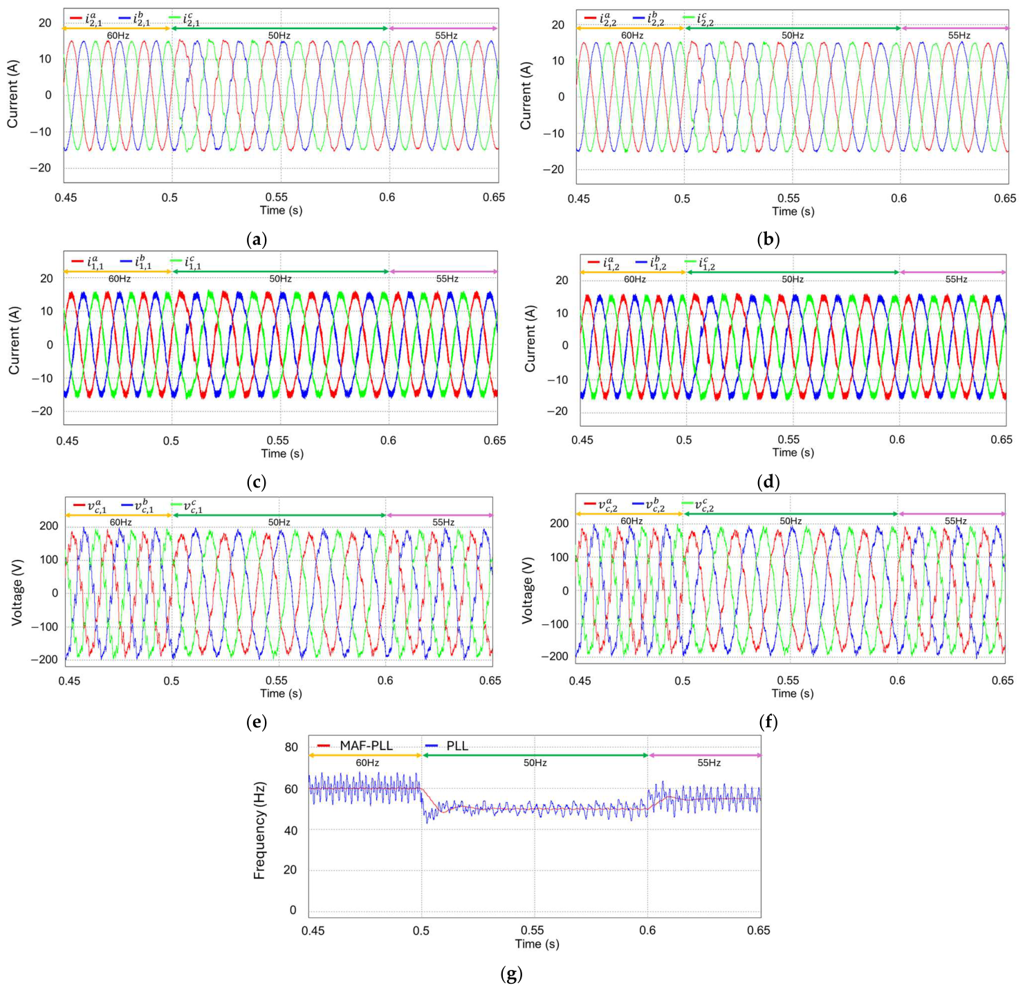
Figure 15 presents the transient responses of the multiple GCIs during the grid frequency transitions to 50 Hz and 55 Hz, at 0.5 s and 0.6 s, respectively. Figure 15a–f show the grid-side and inverter-side currents together with the capacitor voltages, for inverter #1 and #2, respectively. At the instance of the frequency variations, the grid-injected currents are distorted. However, the phase current waveforms rapidly become stable and sinusoidal after each frequency change. These results demonstrate that the designed frequency-adaptive current control ensures a stable operation and reliable dynamic response despite the grid frequency transitions and harsh grid condition. Figure 15g compares the grid frequency detection results with the MAF-PLL in [21] and the conventional PLL. The comparison result indicates that the MAF-PLL provides a more stable and accurate frequency detection under harsh grid conditions.

Figure 15. Simulation results for transient responses of the multiple GCIs when both inverter #1 and inverter #2 are in operation under grid frequency variations at 0.5 s and 0.6 s. (a) Grid-side currents of inverter #1; (b) grid-side currents of inverter #2; (c) inverter-side currents of inverter #1; (d) inverter-side currents of inverter #2; (e) capacitor voltages of inverter #1; (f) capacitor voltages of inverter #2; (g) grid frequency detection by the MAF-PLL and conventional PLL.

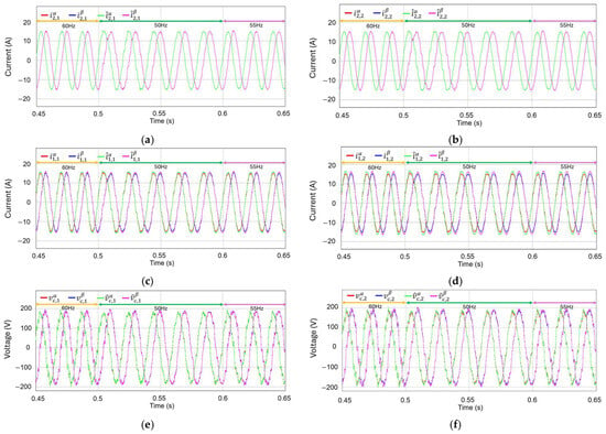
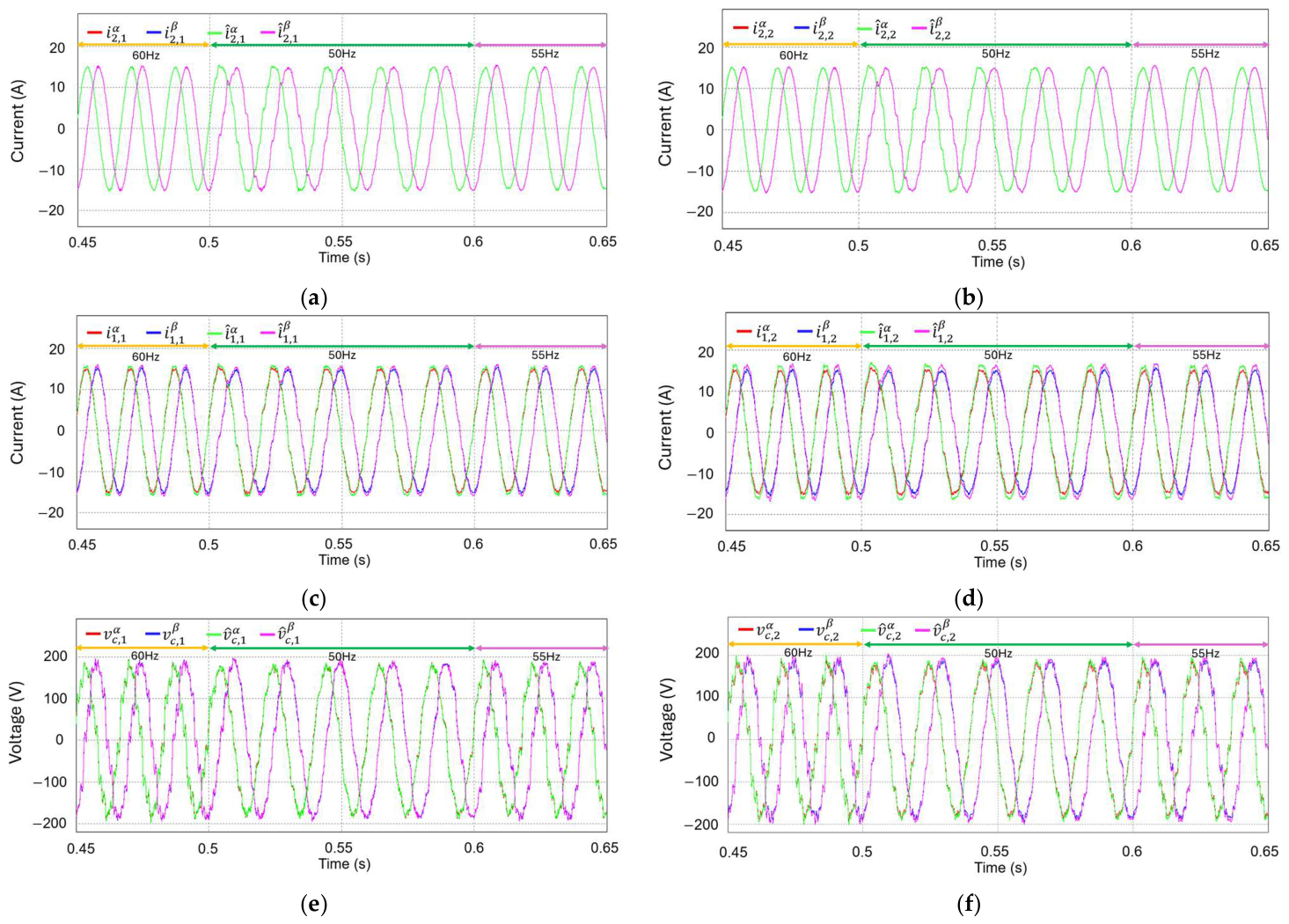
Figure 16 presents the estimation performance of the KF-based current observer under distorted PCC voltages and grid frequency transitions to 50 Hz and 55 Hz, at 0.5 s and 0.6 s, respectively. Figure 16a–f show the measured and estimated waveforms of the grid-side and inverter-side currents together with the capacitor voltages, for inverters #1 and #2, respectively. After each frequency change, the estimated waveforms rapidly become consistent with the measured waveforms. These results confirm accurate state estimation performance of the KF-based current observer even under harsh grid conditions and noisy measurement environments.

Figure 16. Measured and estimated waveforms of the current observer when both inverter #1 and inverter #2 are in operation under grid frequency variations at 0.5 s and 0.6 s. (a) Grid-side currents of inverter #1; (b) grid-side currents of inverter #2; (c) inverter-side currents of inverter #1; (d) inverter-side currents of inverter #2; (e) capacitor voltages of inverter #1; (f) capacitor voltages of inverter #2.

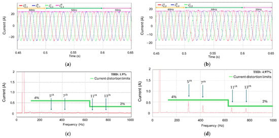
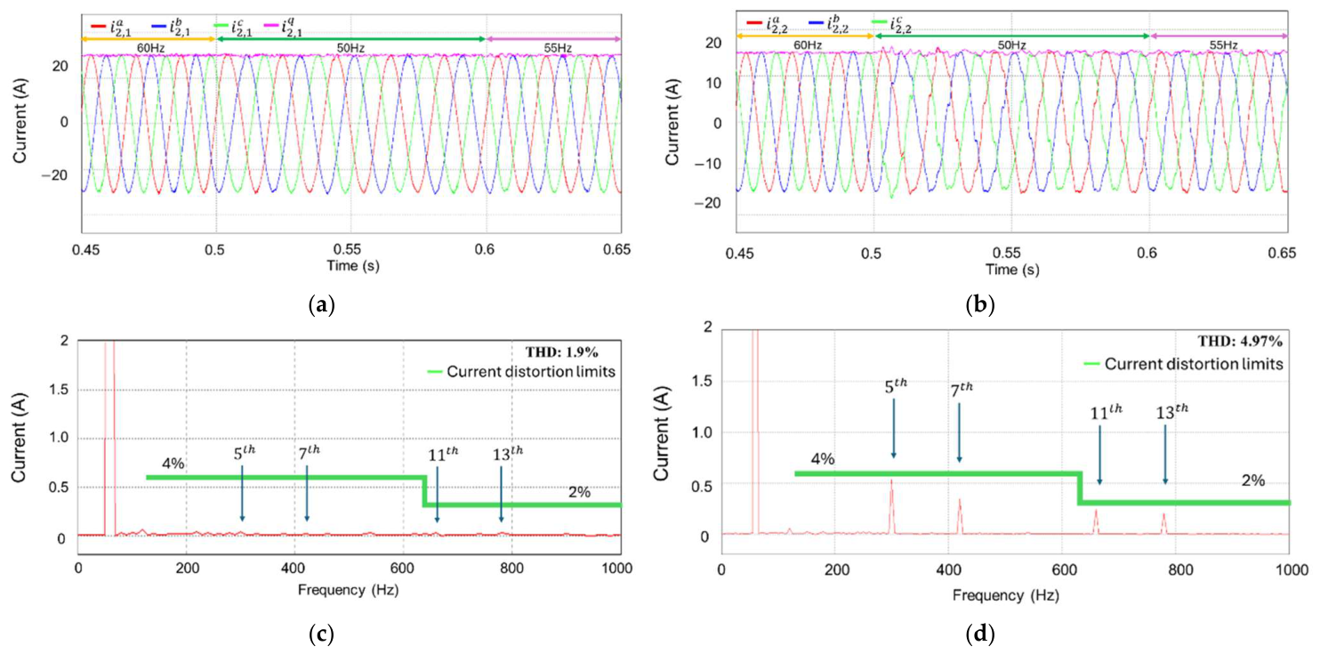
To emphasize the effectiveness of the proposed scheme, Figure 17 presents the comparison results for the main components of the proposed control scheme under the same operating conditions. Figure 17a,b compare the grid-side current responses for fixed-frequency resonant control and frequency-adaptive resonant control, respectively. This comparison shows the effect of frequency-adaptive control on the current response during the grid frequency transitions from 60 Hz to 50 Hz, and then to 55 Hz. Figure 17c,d compare the FFT results of the grid-side current without and with resonant states, respectively. This comparison shows the effect of resonant states on the dominant low-order harmonic components caused by distorted grid voltages.

Figure 17. Comparison results for the main components of the proposed control scheme under the same operating conditions when inverters #1 and #2 are in operation. (a) Grid-side current responses for inverter #1 using frequency-adaptive resonant control; (b) grid-side current responses for inverter #1 using the fixed-frequency resonant control; (c) FFT result of the grid-side current in phase $a$ for inverter #1 with resonant states; (d) FFT result of the grid-side current in phase $a$ for inverter #1 without resonant states.

Table 3 summarizes the quantitative comparison results for the main components of the proposed control scheme under the same operating conditions. Table 3 includes the maximum frequency fluctuation in PLL, phase current THD, observer RMS estimation error, overshoot, and settling time. In Table 3, the MAF-PLL reduces the maximum frequency fluctuation from $\pm$7 Hz to $\pm$1.1 Hz. While the fixed frequency in the resonant controller produces the current THD of 15.4%, the proposed adaptive controller with the detected grid frequency based on the MAF-PLL reduces the current THD to 1.9%. The THD values in the output current without and with the resonant states are 4.97% and 1.9%, respectively. In addition, the KF-based observer yields an RMS estimation error of 0.0001 A, whereas the conventional and LQR-based observers produce RMS estimation errors of 1.3 A and 0.0003 A, respectively. For the $q$-axis current reference step change from 10 A to 15 A, the proposed controller shows an overshoot of 7.3% and a settling time of 0.001 s. These quantitative results demonstrate that the proposed control scheme improves frequency detection, current THD, harmonic suppression, state estimation accuracy, and transient response under the same operating conditions.

Table 3. Quantitative comparison results for the main components of the proposed control scheme.

	Methods	Evaluation Criteria	Value
Other control schemes for comparison [15,43,44,45]	PLL	Maximum frequency fluctuation	$\pm$7 Hz
	With fixed grid frequency	Current THD	15.4%
	Without resonant control	Current THD	4.97%
	Conventional observer	RMS estimation error	1.3 A
	LQR-based observer	RMS estimation error	0.0003 A
Proposed control scheme	MAF-PLL	Maximum frequency fluctuation	$\pm$1.1 Hz
	With frequency-adaptive scheme	Current THD	1.9%
	With resonant control	Current THD	1.9%
	KF-based observer	RMS estimation error	0.0001 A
	$q$-axis current reference step from 10 A to 15 A	Overshoot	7.3%
		Settling time	0.001 s

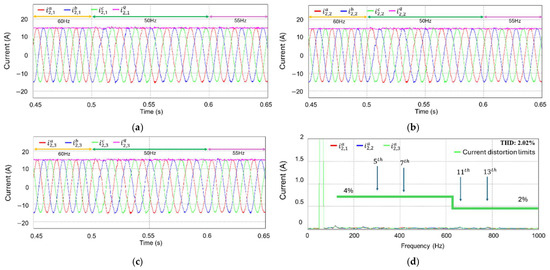
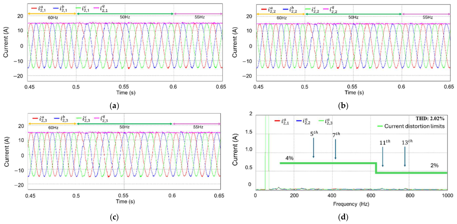
To further examine the applicability of the proposed method, additional simulation is performed with three parallel GCIs under harsh grid conditions and grid frequency variation. Figure 18 presents the grid-side current responses of three parallel GCIs and the FFT results of $a$-phase grid-side currents. As shown in Figure 18, all three GCIs maintain the reference current tracking without unstable oscillation or current distortion caused by interactions among the parallel GCIs. The FFT results also confirm that the dominant harmonic components remain suppressed in the three parallel GCIs, with the current THD remaining at 2.02%. This simulation test proves that the proposed control scheme can be applied stably for three parallel GCIs.

Figure 18. Simulation results for three parallel GCIs under the harsh grid condition. (a) Grid-side current of inverter #1; (b) grid-side current of inverter #2; (c) grid-side current of inverter #3; (d) FFT results of the $a$-phase grid-side currents of inverters #1, #2, and #3.

6. Experimental Results

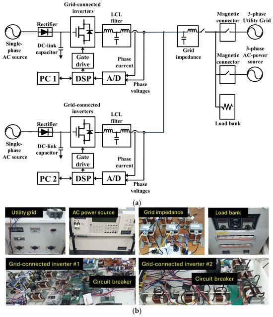
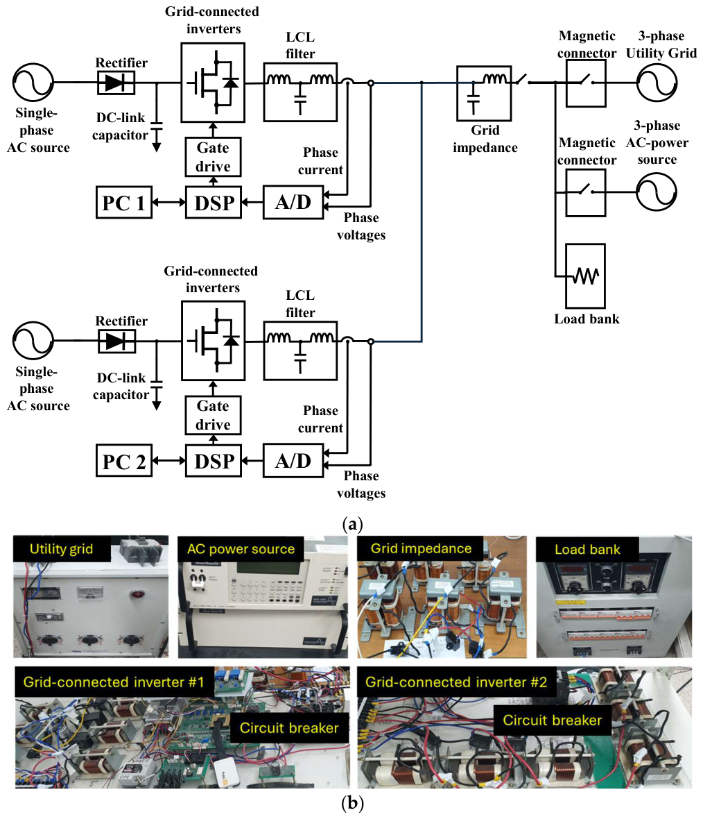
Hardware experiments are conducted with the laboratory parallel multiple GCI system in Figure 19 to assess the current controller described in this study. Figure 19a shows the experimental arrangement, which is composed of two inverter units and the grid connection. The parallel multiple GCI system is also connected to the load bank, the grid impedance, and the magnetic contactor. In this study, a three-phase real utility grid and a three-phase AC power source are employed. Most experiments are conducted in the environment of three-phase real utility grid. Frequency adaptation performance of the current control is tested with three-phase AC power source.

Figure 19. Hardware implementation. (a) Overall system structure; (b) photograph of the experimental hardware setup.

Inverter unit #1 and inverter unit #2 have the same structure, and each unit contains a single-phase AC source, a rectifier, a DC-link capacitor, a grid-connected inverter, an LCL filter, a gate driver circuit, an analog-to-digital converter, and a DSP TMS320F28335. The outputs of the two inverter units are connected to the PCC for parallel operation. The PCC voltage and grid-side current signals measured in each unit are transmitted to the corresponding DSP through the analog-to-digital converter. To evaluate the robustness of the system under more severe measurement noise condition, measurement noise is further superimposed on the sampled current and PCC voltage signals. Figure 19b shows the photograph of the experimental hardware setup.

Table 4 presents the measured execution times of the proposed control scheme in the DSP at a sampling frequency of 10 kHz. The overall control algorithm requires 77 μs, which is shorter than the sampling time of 100 μs. Therefore, the proposed control algorithm can be implemented in real time using a commercial DSP.

Table 4. Execution times of the proposed control scheme.

Full algorithm	77 $\mathsf{\mu }\mathrm{s}$
Data acquisition, MAF-PLL	40 $\mathsf{\mu }\mathrm{s}$
Space vector modulation	10 $\mathsf{\mu }\mathrm{s}$
KF-based current observer	21 $\mathsf{\mu }\mathrm{s}$
State-feedback current controller	6 $\mathsf{\mu }\mathrm{s}$

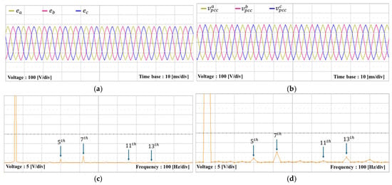
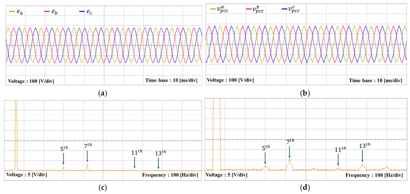
Figure 20a shows three-phase grid voltage waveforms, and Figure 20b presents the three-phase PCC voltage waveforms under LC grid impedance. Figure 20c,d present the FFT results in phase $a$ of the grid and PCC voltages, respectively. These results indicate that the LC grid impedance increases the voltage distortion at the PCC. The proposed current controller is evaluated under this distorted PCC voltage condition.

Figure 20. Grid and PCC voltages of the utility grid for the experiments. (a) Grid voltages; (b) PCC voltages; (c) FFT result for grid voltage in phase $a$; (d) FFT result for PCC voltage in phase $a$.

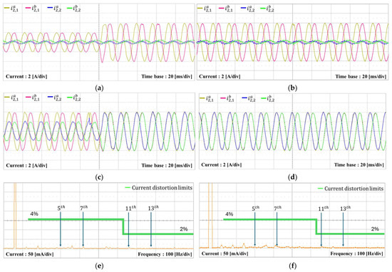
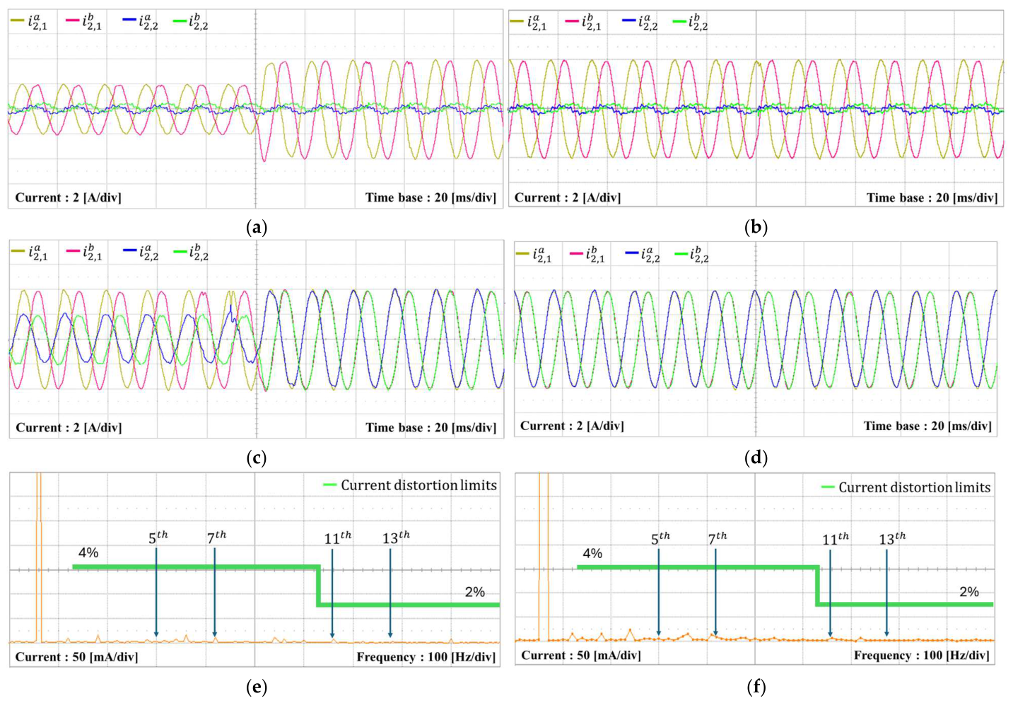
Figure 21 presents the experimental current responses under distorted PCC voltages. Figure 21a,b show the grid-side current responses when inverter #1 operates, while inverter #2 remains inactive. Inverter #1 operates with the current reference of 2 A in Figure 21a, and the reference increases to 4 A in Figure 21b. Figure 21c,d show the current responses when inverter #2 begins operation in parallel while inverter #1 maintains the current of 4 A. Inverter #2 operates with the current reference of 2 A in Figure 21c, and its reference increases to 4 A in Figure 21d. Figure 21e,f illustrate the FFT results for the grid-side current in phase $a$ of inverter #1 and inverter #2, respectively. These FFT results confirm that the steady-state current quality satisfies the limits specified in [3]. As a result, it is proved that the proposed current controller maintains a stable current control performance and effective harmonic suppression in multiple GCIs under distorted PCC voltages.

Figure 21. Experimental results of the current responses under distorted PCC voltages. (a) Transient response of grid-side currents of inverter #1 when inverter #2 is in idle mode; (b) steady-state grid-side currents of inverter #1 when inverter #2 is in idle mode; (c) transient response of grid-side currents of inverter #2 under steady-state condition of inverter #1; (d) steady-state grid-side currents of inverter #1 and #2; (e) FFT result for grid-side current in phase $a$ of inverter #1; (f) FFT result for grid-side current in phase $a$ of inverter #2.

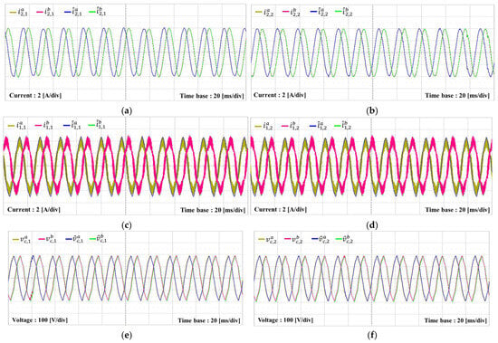
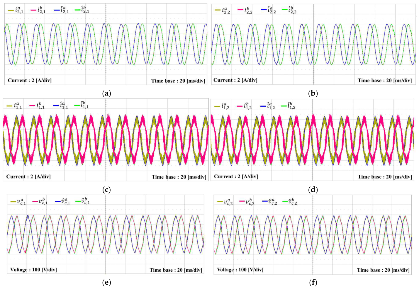
Figure 22 presents the experimental results for the measured and estimated variables with the KF-based current observer when both inverters operate in parallel. To verify the estimation performance using the hardware test, the measured and estimated waveforms of inverter #1 and #2 are compared when both inverters operate in parallel. Figure 22a–f show the grid-side and inverter-side currents together with the capacitor voltages in inverter #1 and #2, respectively. These results demonstrate that the proposed KF-based current observer provides a reliable state estimation.

Figure 22. Measured and estimated experimental results of the KF-based current observer when both inverter #1 and inverter #2 are in operation under distorted PCC voltages. (a) Estimation of grid-side currents of inverter #1; (b) estimation of grid-side currents of inverter #2; (c) estimation of inverter-side currents of inverter #1; (d) estimation of inverter-side currents of inverter #2; (e) estimation of capacitor voltages of inverter #1; (f) estimation of capacitor voltages of inverter #2.

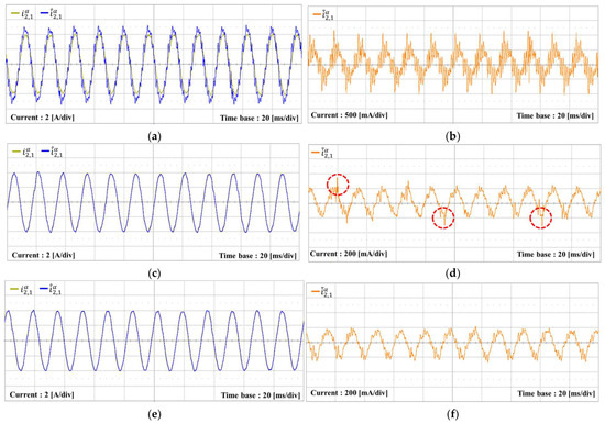
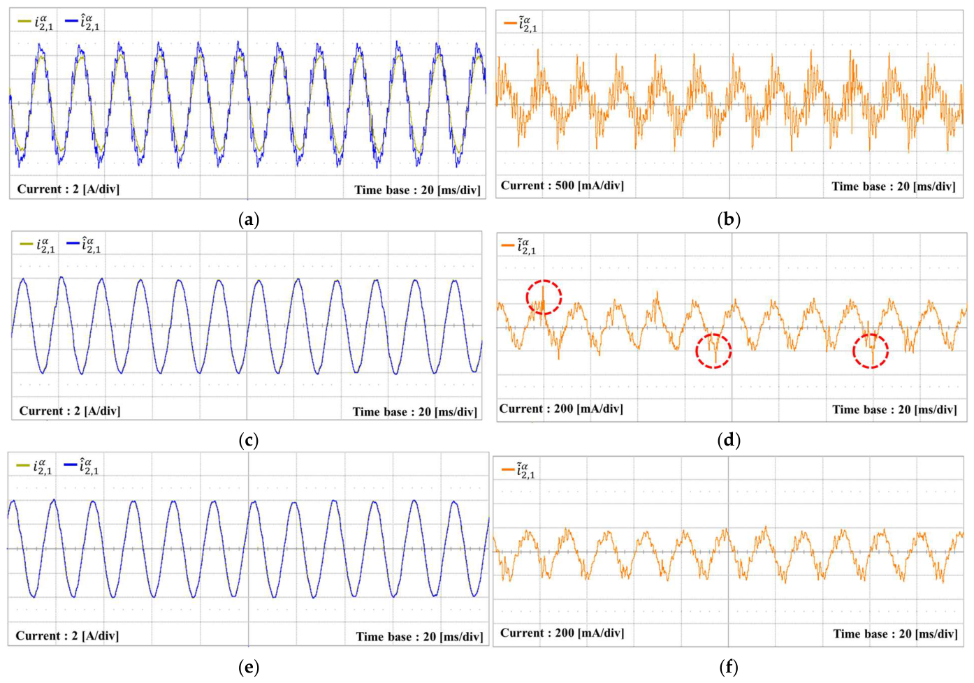
Figure 23 shows the experimental comparison of the estimation performance for different observers implemented in the stationary reference frame under noisy measurement conditions. Figure 23a,c,e show the measured and estimated values for the conventional observer, LQR-based observer, and KF-based observer, respectively. Figure 23b,d,f show the estimation errors between the measured and estimated values for each observer. The results indicate that the KF-based observer provides more reliable estimated states for the state-feedback current controller under measurement noise environment.

Figure 23. Experimental comparison of the estimation performance for different observers implemented in the stationary reference frame under noisy measurement conditions. (a) Measured and estimated values of the conventional observer; (b) estimation error of the conventional observer; (c) measured and estimated values of the LQR-based observer; (d) estimation error of the LQR-based observer; (e) measured and estimated values of the KF-based observer; (f) estimation error of the KF-based observer. The red dotted circles in (d) indicate intermittent spikes in the estimation error of the LQR-based observer.

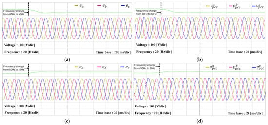
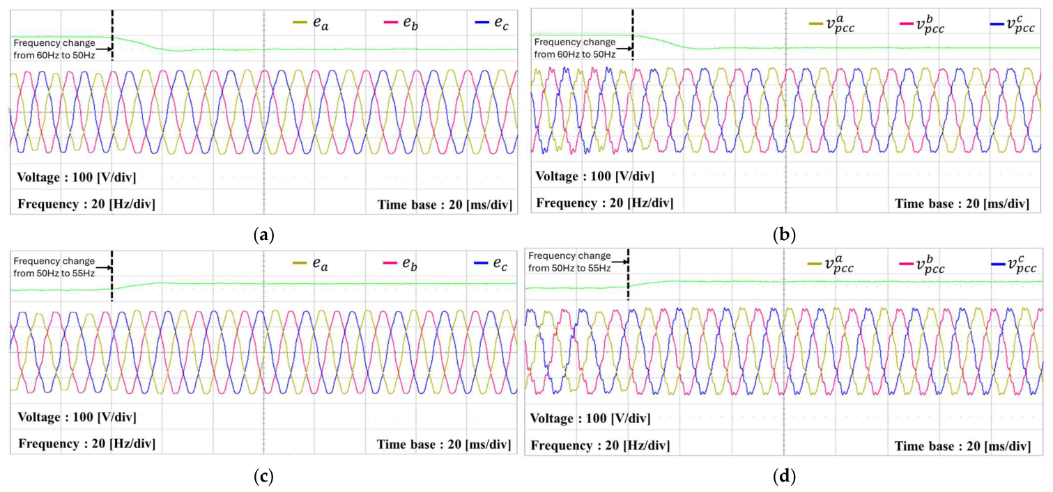
Figure 24 presents the grid and PCC voltages under grid conditions including distortion, imbalance, and frequency variation. Figure 24a,b present the grid voltages and PCC voltages, respectively, during the grid frequency transition from 60 Hz to 50 Hz. Figure 24c,d present the grid voltages and PCC voltages, respectively, during the frequency transition from 50 Hz to 55 Hz. It is shown that the experimental voltage conditions include distorted voltages, unbalanced voltages, and grid frequency variations. These voltages are used to assess how the proposed controller operates under harsh grid conditions.

Figure 24. Grid and PCC voltages under voltage distortion, voltage imbalance, and grid frequency variations. (a) Grid voltages with frequency variation from 60 Hz to 50 Hz; (b) PCC voltages with frequency variation from 60 Hz to 50 Hz; (c) grid voltages with frequency variation from 50 Hz to 55 Hz; (d) PCC voltages with frequency variation from 50 Hz to 55 Hz. The green line indicates the grid frequency.

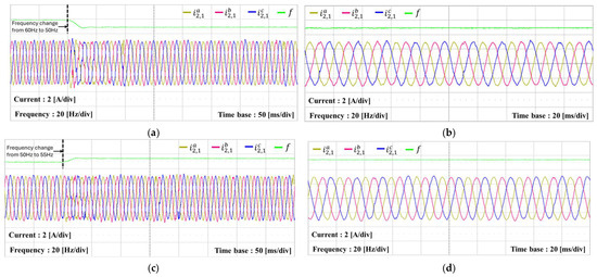
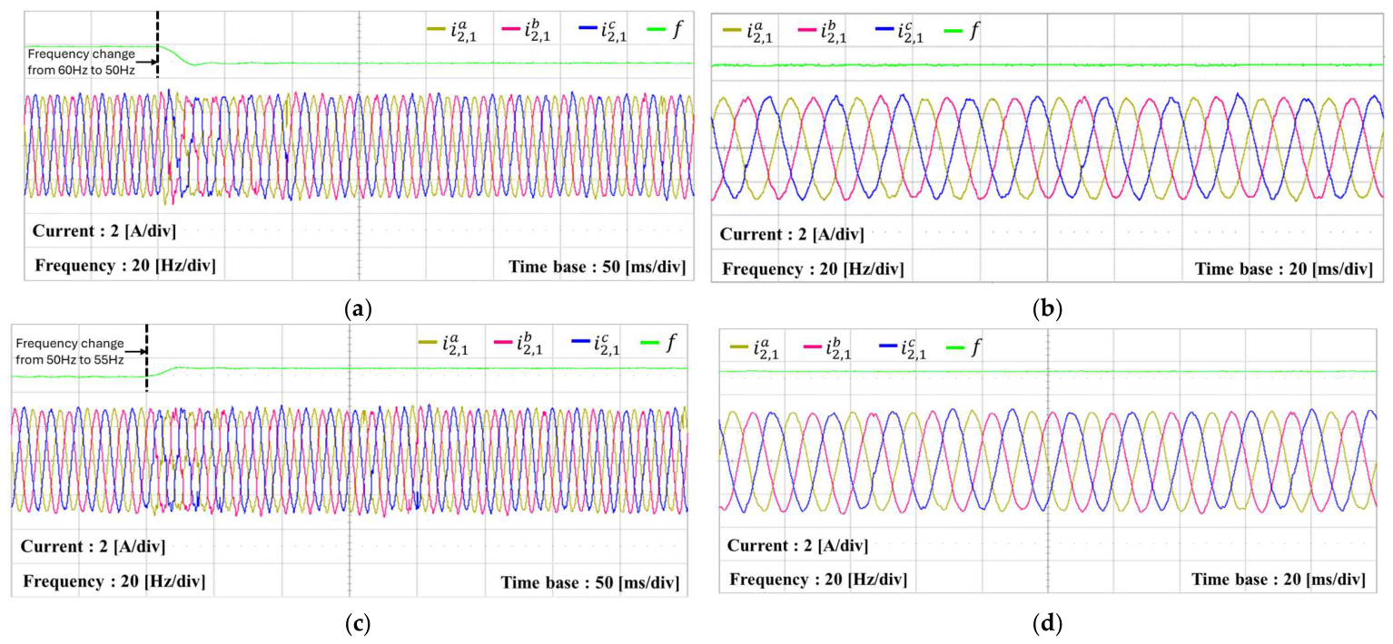
Figure 25 presents the experimental current responses of inverter #1 under the grid frequency transition in parallel operation, where current references of 3 A and 1 A are assigned to inverter #1 and inverter #2, respectively. Figure 25a,c present the grid-side currents when the grid frequency changes from 60 Hz to 50 Hz and from 50 Hz to 55 Hz, respectively, whereas Figure 25b,d show the corresponding steady-state currents after each transition. In both cases, the proposed scheme has fast transient responses during the frequency transition and maintains stable sinusoidal waveforms after each transition. These responses demonstrate that the current controller maintains stable current regulation and current quality despite the grid frequency transition.

Figure 25. Experimental results of current responses for inverter #1 under frequency variation. (a) Grid-side currents of inverter #1 under frequency variation from 60 Hz to 50 Hz; (b) grid-side currents of inverter #1 at steady-state after the frequency change to 50 Hz; (c) grid-side currents of inverter #1 under frequency variation from 50 Hz to 55 Hz; (d) grid-side currents of inverter #1 at steady-state after the frequency change to 55 Hz.

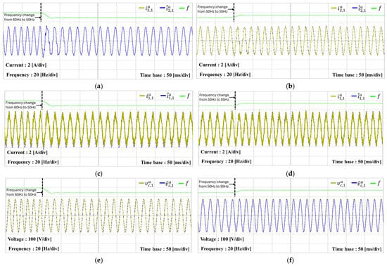
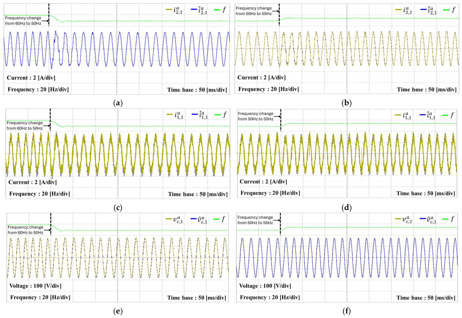
Figure 26 presents the estimation performance of the KF-based current observer by experiment when inverter #1 and inverter #2 operate simultaneously under grid frequency variations. Figure 26a–f show the grid-side and inverter-side currents together with the capacitor voltages when the grid frequency changes from 60 Hz to 50 Hz and from 50 Hz to 55 Hz, respectively. At the instance of the frequency changes, slight deviations appear between the measured and estimated waveforms. However, the estimated values rapidly converge to the measured values after each frequency change. The results confirm that the proposed current observer maintains accurate state estimation performance even under grid frequency variations.

Figure 26. Measured and estimated experimental results of the KF-based current observer when both inverter #1 and inverter #2 are in operation under frequency variation. (a) Estimation of grid-side current in phase $a$ of inverter #1 under frequency variation from 60 Hz to 50 Hz; (b) estimation of grid-side current in phase $a$ of inverter #1 under frequency variation from 50 Hz to 55 Hz; (c) estimation of inverter-side current in phase $a$ of inverter #1 under frequency variation from 60 Hz to 50 Hz; (d) estimation of inverter-side current in phase $a$ of inverter #1 under frequency variation from 50 Hz to 55 Hz; (e) estimation of capacitor voltages in phase $a$ of inverter #1 under frequency variation from 60 Hz to 50 Hz; (f) estimation of capacitor voltages in phase $a$ of inverter #1 under frequency variation from 50 Hz to 55 Hz.

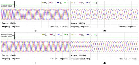
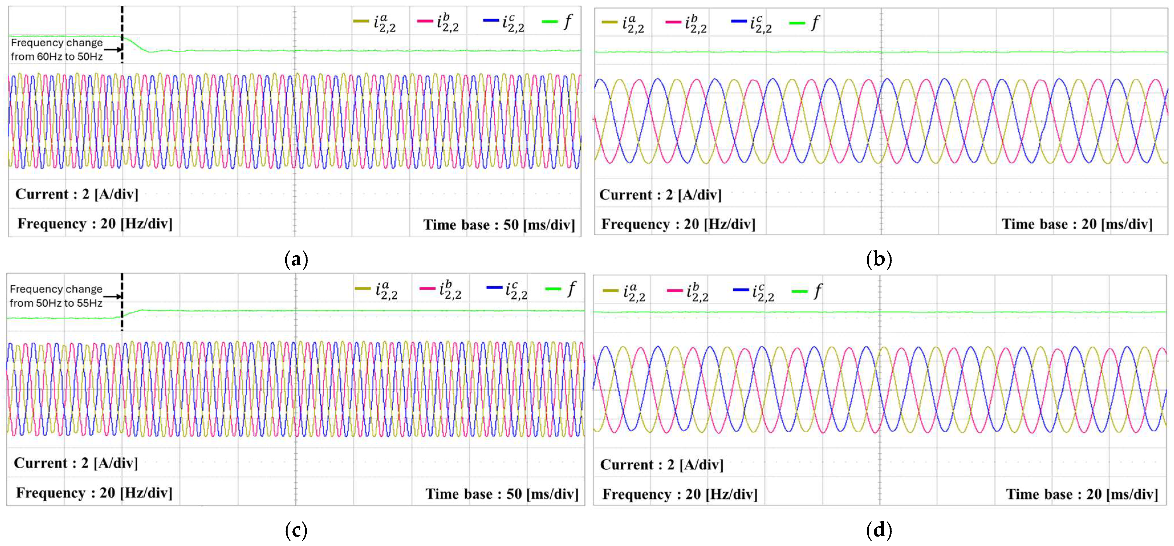
Figure 27 presents the experimental current responses of inverter #2 under the grid frequency variations. Under parallel operation, inverter #1 operates with the current reference of 1 A, whereas inverter #2 operates with 3 A. Similarly, the current response of inverter #2 is also evaluated under two grid frequency transitions, one from 60 Hz to 50 Hz and the other from 50 Hz to 55 Hz. In both cases, inverter #2 operates reliably in multiple GCI configuration and maintains stable current responses under the grid frequency variations.

Figure 27. Experimental results of current responses for inverter #2 under frequency variation. (a) Grid-side currents of inverter #2 under frequency variation from 60 Hz to 50 Hz; (b) grid-side currents of inverter #2 at steady-state after the frequency change to 50 Hz; (c) grid-side currents of inverter #2 under frequency variation from 50 Hz to 55 Hz; (d) grid-side currents of inverter #2 at steady-state after the frequency change to 55 Hz.

Table 5 presents the current overshoot, settling time, and observer convergence time of Figure 25, Figure 26 and Figure 27 during the grid frequency transitions. The maximum current overshoot is 0.6 A, and the maximum settling time is 38 ms under the tested frequency transitions. In addition, with the KF-based observer, the estimated currents converge to the measured values within 20 ms after each frequency transition. These quantitative results support the waveforms in Figure 25, Figure 26 and Figure 27 and confirm that the proposed control scheme maintains stable current control and reliable state estimation during grid frequency changes.

Table 5. Quantitative performance results under grid frequency transitions.

	Frequency Change	Current Overshoot	Settling Time	Convergence Time
Inverter #1 current response in Figure 25	60 Hz to 50 Hz	0.6 A	38 ms	$-$
	50 Hz to 55 Hz	0.4 A	30 ms	$-$
Inverter #2 current response in Figure 27	60 Hz to 50 Hz	0.2 A	25 ms	$-$
	50 Hz to 55 Hz	0.2 A	20 ms	$-$
KF-based observer response in Figure 26	60 Hz to 50 Hz	$-$	$-$	20 ms
	50 Hz to 55 Hz	$-$	$-$	20 ms

Note: The minus sign (−) indicates not applicable.

7. Conclusions

This paper has developed a frequency-adaptive current control scheme based on a Kalman filter-based observer for parallel multiple GCIs under harsh grid conditions and LC-type grid impedance. First, a state model is represented for a parallel GCI system under the LC grid impedance. Based on the developed model, a current controller is constructed in a state-feedback framework with integral action and resonant compensators to ensure accurate reference current tracking and harmonic compensation. A Kalman filter-based observer is adopted to estimate the state variables for feedback control and improve the estimation accuracy under noisy measurement conditions. In addition, the MAF-PLL maintains accurate tracking of the grid frequency and phase even under harsh grid conditions to ensure an effective frequency-adaptive current control design. An admittance-based stability analysis is then used to assess the coupling among the inverters operating in parallel and the grid influence on overall system operation. The analytical results, PSIM simulations, and hardware experiments validate the applicability of the proposed control method under voltage imbalance, voltage distortion, grid frequency variation, and LC grid impedance. The simulation results show that the grid-side current THD is reduced to 1.9% under the tested harsh grid condition. The KF-based observer also reduces the RMS estimation error to 0.0001 A under noisy measurement conditions. The dynamic responses measured in the hardware experiments under grid frequency transitions show a maximum current overshoot of 0.6 A, a settling time of 38 ms, and an observer convergence time of 20 ms. These numerical data clearly support a stable parallel operation, reliable state estimation, accurate reference current tracking, and effective harmonic suppression of the proposed scheme. The proposed method is validated under LC grid impedance, voltage distortion, voltage imbalance, and grid frequency transition conditions. To validate multiple GCI systems under more diverse conditions, non-identical inverter parameters and different grid impedance values can be considered as future work.

References

- Zahedi, A. A review of drivers, benefits, and challenges in integrating renewable energy sources into electricity grid. Renew. Sustain. Energy Rev. 2011, 15, 4775–4779. [Google Scholar] [CrossRef] [Scilit]
- Iweh, C.D.; Gyamfi, S.; Tanyi, E.; Effah-Donyina, E. Distributed generation and renewable energy integration into the grid: Prerequisites, push factors, practical options, issues and merits. Energies 2021, 14, 5375. [Google Scholar] [CrossRef] [Scilit]
- IEEE Std 1547-2018; IEEE Standard for Interconnection and Interoperability of Distributed Energy Resources with Associated Electric Power Systems Interfaces. IEEE: New York, NY, USA, 2018. [CrossRef] [Scilit]
- Boscaino, V.; Ditta, V.; Marsala, G.; Panzavecchia, N.; Tinè, G.; Cosentino, V.; Cataliotti, A.; Di Cara, D. Grid-connected photovoltaic inverters: Grid codes, topologies and control techniques. Renew. Sustain. Energy Rev. 2024, 189, 113903. [Google Scholar] [CrossRef] [Scilit]
- Liserre, M.; Blaabjerg, F.; Hansen, S. Design and control of an LCL-filter-based three-phase active rectifier. IEEE Trans. Ind. Appl. 2005, 41, 1281–1291. [Google Scholar] [CrossRef] [Scilit]
- Peña-Alzola, R.; Liserre, M.; Blaabjerg, F.; Ordonez, M.; Yang, Y. LCL-filter design for robust active damping in grid-connected converters. IEEE Trans. Ind. Inform. 2014, 10, 2192–2203. [Google Scholar] [CrossRef] [Scilit]
- Beres, R.N.; Wang, X.; Liserre, M.; Blaabjerg, F.; Bak, C.L. A review of passive power filters for three-phase grid-connected voltage-source converters. IEEE J. Emerg. Sel. Top. Power Electron. 2016, 4, 54–69. [Google Scholar] [CrossRef] [Scilit]
- Jia, X.; Yu, S.; Zhang, Y.; Feng, Y.; Zhou, B. LCL grid-connected inverter resonance feedforward-active damping hybrid control strategy for mitigating weak grid resonance and harmonic currents. Energies 2025, 18, 6010. [Google Scholar] [CrossRef] [Scilit]
- Hu, Z.; Xing, X.; Wang, H.; Li, Z.; Li, Y.; Blaabjerg, F. Modeling and delay compensation method for improving the stability of grid-connected inverter with LCL filter under weak grid conditions. IEEE Trans. Power Electron. 2026, 41, 6111–6124. [Google Scholar] [CrossRef] [Scilit]
- Dannehl, J.; Fuchs, F.W.; Thøgersen, P.B. PI state space current control of grid-connected PWM converters with LCL filters. IEEE Trans. Power Electron. 2010, 25, 2320–2330. [Google Scholar] [CrossRef] [Scilit]
- Dirscherl, C.; Fessler, J.; Hackl, C.M.; Ipach, H. State-feedback controller and observer design for grid-connected voltage source power converters with LCL-filter. In Proceedings of the 2015 IEEE Conference on Control Applications (CCA), Sydney, Australia, 21–23 September 2015; pp. 215–222. [Google Scholar] [CrossRef] [Scilit]
- Kukkola, J.; Hinkkanen, M.; Zenger, K. Observer-based state-space current controller for a grid converter equipped with an LCL filter: Analytical method for direct discrete-time design. IEEE Trans. Ind. Appl. 2015, 51, 4079–4090. [Google Scholar] [CrossRef] [Scilit]
- Kukkola, J.; Hinkkanen, M. Observer-based state-space current control for a three-phase grid-connected converter equipped with an LCL filter. IEEE Trans. Ind. Appl. 2014, 50, 2700–2709. [Google Scholar] [CrossRef] [Scilit]
- Wang, B.; Xu, Y.; Shen, Z.; Zou, J.; Li, C.; Liu, H. Current control of grid-connected inverter with LCL filter based on extended-state observer estimations using single sensor and achieving improved robust observation dynamics. IEEE Trans. Ind. Electron. 2017, 64, 5428–5439. [Google Scholar] [CrossRef] [Scilit]
- Kim, S.-D.; Tran, T.V.; Yoon, S.-J.; Kim, K.-H. Current controller design of grid-connected inverter with incomplete observation considering L-/LC-type grid impedance. Energies 2024, 17, 1855. [Google Scholar] [CrossRef] [Scilit]
- Zheng, F.; Wu, W.; Chen, B.; Koutroulis, E. An optimized parameter design method for passivity-based control in a LCL-filtered grid-connected inverter. IEEE Access 2020, 8, 189878–189890. [Google Scholar] [CrossRef] [Scilit]
- Eldeeb, H.; Massoud, A.; Abdel-Khalik, A.S.; Ahmed, S. A sensorless Kalman filter-based active damping technique for grid-tied VSI with LCL filter. Int. J. Electr. Power Energy Syst. 2017, 93, 146–155. [Google Scholar] [CrossRef] [Scilit]
- Lu, M.; Yang, Y.; Johnson, B.; Blaabjerg, F. An interaction-admittance model for multi-inverter grid-connected systems. IEEE Trans. Power Electron. 2019, 34, 7542–7557. [Google Scholar] [CrossRef] [Scilit]
- Chen, T.; Lee, C.K.; Hui, S.Y.R. A general design procedure for multi-parallel modular grid-tied inverters system to prevent common and interactive instability. IEEE Trans. Power Electron. 2019, 34, 6025–6030. [Google Scholar] [CrossRef] [Scilit]
- Gao, C.; Chen, J.; Wu, W.; Lu, G.; Koutroulis, E.; Blaabjerg, F. A New Control Strategy with Simplified Model and Kalman Filter Estimator for Grid-Tied Inverter with Asymmetric LCL Filter. In Proceedings of the IECON 2022–48th Annual Conference of the IEEE Industrial Electronics Society, Brussels, Belgium, 17–20 October 2022; pp. 1–6. [Google Scholar] [CrossRef] [Scilit]
- Yang, Y.; Zhou, K.; Wang, H.; Blaabjerg, F.; Wang, D.; Zhang, B. Frequency adaptive selective harmonic control for grid-connected inverters. IEEE Trans. Power Electron. 2015, 30, 3912–3924. [Google Scholar] [CrossRef] [Scilit]
- Ye, J.; Liu, L.; Xu, J.; Shen, A. Frequency adaptive proportional-repetitive control for grid-connected inverters. IEEE Trans. Ind. Electron. 2021, 68, 7965–7974. [Google Scholar] [CrossRef] [Scilit]
- Xiao, F.; Dong, L.; Li, L.; Liao, X. A Frequency-Fixed SOGI-Based PLL for Single-Phase Grid-Connected Converters. IEEE Trans. Power Electron. 2017, 32, 1713–1719. [Google Scholar] [CrossRef] [Scilit]
- Ali, Z.; Christofides, N.; Hadjidemetriou, L.; Kyriakides, E.; Yang, Y.; Blaabjerg, F. Three-phase phase-locked loop synchronization algorithms for grid-connected renewable energy systems: A review. Renew. Sustain. Energy Rev. 2018, 90, 434–452. [Google Scholar] [CrossRef] [Scilit]
- Golestan, S.; Ramezani, M.; Guerrero, J.M.; Freijedo, F.D.; Monfared, M. Moving average filter based phase-locked loops: Performance analysis and design guidelines. IEEE Trans. Power Electron. 2014, 29, 2750–2763. [Google Scholar] [CrossRef] [Scilit]
- Wang, Z.; Fu, P.; Huang, L.; Chen, X.; He, S.; Zhang, X.; Yang, J. Performance improvement of a three-phase PLL under distorted grid conditions based on frequency adaptive hybrid pre-filtering. IET Power Electron. 2022, 15, 1429–1440. [Google Scholar] [CrossRef] [Scilit]
- Li, Q.; Sun, P.; Dong, G.; Chen, Y. Resonance coupling analysis of multiple differently parameterized grid-connected inverters in new energy generation. Int. J. Electr. Power Energy Syst. 2024, 156, 109743. [Google Scholar] [CrossRef] [Scilit]
- Lu, M.; Wang, X.; Loh, P.C.; Blaabjerg, F. Resonance interaction of multi-parallel grid-connected inverters with LCL filter. IEEE Trans. Power Electron. 2017, 32, 894–899. [Google Scholar] [CrossRef] [Scilit]
- Li, J.; Song, S.; Li, R.; Sun, W. Analysis of active impedance characteristics and harmonic deterioration of multiple grid connected inverters considering nonlinear factors. IET Renew. Power Gener. 2024, 18, 3429–3442. [Google Scholar] [CrossRef] [Scilit]
- Cao, W.; Wang, S.; Kang, H.; Liu, K.; Wang, Q.; Zhao, J. Inherent interaction analysis for harmonic oscillations in the multi-paralleled grid-connected inverter system using a sum type criterion: Global admittance (GA). IEEE Access 2020, 8, 8275–8285. [Google Scholar] [CrossRef] [Scilit]
- Sun, J. Impedance-based stability criterion for grid-connected inverters. IEEE Trans. Power Electron. 2011, 26, 3075–3078. [Google Scholar] [CrossRef] [Scilit]
- Tran, T.V.; Kim, K.-H. Stability Improvement of Parallel-Connected Inverters Under Very Weak Distorted Grid Using Observer-Based Incremental Control Scheme. IEEE Access 2023, 11, 141523–141536. [Google Scholar] [CrossRef] [Scilit]
- Orellana, L.; Sainz, L.; Prieto Araujo, E.; Gomis Bellmunt, O. Stability assessment for multi-infeed grid-connected VSCs modeled in the admittance matrix form. IEEE Trans. Circuits Syst. I Regul. Pap. 2021, 68, 3758–3771. [Google Scholar] [CrossRef] [Scilit]
- Qiu, Y.; Wang, Y.; Tian, Y.; Chen, Z. Intelligent stability monitoring and improvement of grid-connected converter under weighted average control. IET Smart Grid 2024, 7, 776–788. [Google Scholar] [CrossRef] [Scilit]
- Qiu, Y.; Wang, Y.; Tian, Y.; Chen, Z. An intelligent stability prediction method of grid-connected inverter considering time-varying parameters. IEEE Trans. Ind. Appl. 2024, 60, 3685–3697. [Google Scholar] [CrossRef] [Scilit]
- Franklin, G.F.; Powell, J.D.; Workman, M.L. Digital Control of Dynamic Systems, 3rd ed.; Addison-Wesley: Menlo Park, CA, USA, 1998. [Google Scholar]
- Ogata, K. Discrete-Time Control Systems, 2nd ed.; Prentice Hall: Upper Saddle River, NJ, USA, 1995. [Google Scholar]
- Ama, N.R.N.; Komatsu, W.; Matakas Junior, L. Single and three phase moving average filter PLLs: Digital controller design recipe. Electr. Power Syst. Res. 2014, 116, 276–283. [Google Scholar] [CrossRef] [Scilit]
- Maccari, L.A., Jr.; Santini, A.C.L.; Pinheiro, H.; de Oliveira, R.C.L.F.; Montagner, V.F. Robust Optimal Current Control for Grid-Connected Three-Phase Pulse-Width Modulated Converters. IET Power Electron. 2015, 8, 1490–1499. [Google Scholar] [CrossRef] [Scilit]
- Åkesson, B.M.; Jørgensen, J.B.; Poulsen, N.K.; Jørgensen, S.B. A generalized autocovariance least-squares method for Kalman filter tuning. J. Process Control 2008, 18, 769–779. [Google Scholar] [CrossRef] [Scilit]
- Agorreta, J.L.; Borrega, M.; López, J.; Marroyo, L. Modeling and control of N-paralleled grid-connected inverters with LCL filter coupled due to grid impedance in PV plants. IEEE Trans. Power Electron. 2011, 26, 770–785. [Google Scholar] [CrossRef] [Scilit]
- Wang, X.; Blaabjerg, F.; Loh, P.C. Passivity-based stability analysis and damping injection for multiparalleled VSCs with LCL filters. IEEE Trans. Power Electron. 2017, 32, 8922–8935. [Google Scholar] [CrossRef] [Scilit]
- Tripathy, P.; Misra, B.; Nayak, B. Phase-locked loop based synchronization schemes for three-phase unbalanced and distorted grid: A review. Int. J. Appl. Power Eng. 2024, 13, 934–943. [Google Scholar] [CrossRef] [Scilit]
- Biricik, S.; Komurcugil, H.; Ahmed, H.; Sharifzadeh, M.; Mehrasa, M.; Al-Haddad, K. Proportional-resonant based control strategy for grid-connected packed-E cell inverters with Lyapunov filter-based PLL. IET Gener. Transm. Distrib. 2023, 17, 645–654. [Google Scholar] [CrossRef] [Scilit]
- Gao, C.; Tan, F. A new model reduction method based PBC control for grid-connected inverter with LCL-filter. Sci. Rep. 2024, 14, 21442. [Google Scholar] [CrossRef] [Scilit] [PubMed]
Disclaimer/Publisher’s Note: The statements, opinions and data contained in all publications are solely those of the individual author(s) and contributor(s) and not of MDPI and/or the editor(s). MDPI and/or the editor(s) disclaim responsibility for any injury to people or property resulting from any ideas, methods, instructions or products referred to in the content. |
© 2026 by the authors. Licensee MDPI, Basel, Switzerland. This article is an open access article distributed under the terms and conditions of the Creative Commons Attribution (CC BY) license.