


Abstract
Induction heating is widely used in industrial processes such as forging, hardening, and additive manufacturing, but its accurate numerical simulation requires coupled electromagnetic and thermal finite element analyses with nonlinear, temperature-dependent material properties. This work proposes a deep learning surrogate model based on a convolu-tional neural network for TEAM Workshop Problem 36, a reference benchmark for nonlinear magneto-thermal induction heating. A database of more than 40,000 finite element solutions was generated by varying the supply current from 2 to 6 kA and the frequency from 2 to 6 kHz, while accounting for transient nonlinear effects, including the Curie transition. The network, composed of 24 layers with transposed convolutions, batch normalization, and dropout, maps current, frequency, and time to radial temperature distributions in the steel billet. For most operating conditions, the model achieves mean absolute percentage errors of about 6–7% for radial line in the middle of the billet and about 10% for radial line close to the billet end. Larger discrepancies occur during the early heating stage and near the Curie temperature. Prediction times are reduced by three to four orders of magnitude with respect to a single finite element analysis. The results indicate that the proposed surrogate enables fast temperature estimation for optimization, digital twins, and closed-loop control of induction heating systems.
1. Introduction
The increasing demand for high-performance and energy-efficient manufacturing processes has driven significant research into induction heating technologies over the past decades [1,2]. Compared to conventional resistance or flame-based heating, induction heating is characterized by contactless energy transfer, precise spatial and temporal control of the heat source, and inherently high electrical efficiency [3]. These attributes make it particularly suitable for a wide variety of industrial processes, including billet and bloom forging, surface hardening of mechanical components, brazing of joints, shrink-fitting, and annealing treatments in both ferrous and non-ferrous alloys [4,5]. In modern production lines, induction systems are often integrated into automated cells, where short heating times, repeatability, and ease of control are crucial requirements [1,6]. As a result, the accurate prediction and optimization of process parameters—such as power, frequency, coil geometry, and heating time—have become a central topic in the design of advanced induction equipment [2].
From a physical standpoint, induction heating is intrinsically a multiphysics phenomenon. The process starts with electromagnetic field generation in the inductor, followed by the induction of eddy currents in the workpiece, which in turn give rise to Joule losses and localized volumetric heat sources [6]. The resulting temperature field evolves under the combined action of conduction within the solid, convection at the boundaries, and radiation at high temperatures, often coupled with phase transformations and temperature-dependent material properties [6]. The electromagnetic behavior is further complicated by nonlinear permeability in ferromagnetic regions, skin and proximity effects at medium and high frequencies, and possible changes in geometry (e.g., due to thermal expansion or motion of the workpiece). This complex interplay of electromagnetic and thermal phenomena, compounded by nonlinear, temperature- and field-dependent constitutive laws, makes accurate modeling a formidable challenge.
Moreover, the strong coupling between electromagnetic and thermal domains requires robust numerical procedures capable of accurately capturing temporal variations and spatial gradients.
The TEAM Workshop Problem 36 is a well-known benchmark for induction heating proposed for validation and comparison of coupled magneto-thermal numerical models. Its importance lies in the fact that it combines a well-defined coil–billet geometry with the main challenges of nonlinear magneto-thermal analysis, including temperature-dependent material properties, skin effect, transient heat transfer, and the Curie transition. For this reason, it provides a rigorous and reproducible test case for assessing the accuracy and computational efficiency of numerical and data-driven surrogate models. The benchmark addresses the multi-physics analysis of an induction heating device, characterized by a nonlinear electromagnetic behavior, practical coil–workpiece geometry, and transient thermal effects [7]. Its formulation explicitly couples magneto-quasistatic field computation with time-dependent heat transfer problem, making it a rigorous and challenging test case for advanced modeling techniques. Specifically, the TEAM Problem 36 has become a reference benchmark for assessing the accuracy, robustness, and computational efficiency of finite-element formulations, reduced-order models, surrogate models, and emerging data-driven approaches.
For this benchmark and, more generally, for nonlinear induction heating problems, finite element analysis has long been the gold standard for numerical simulation [8,9]. While highly accurate, FEA is computationally intensive, especially when transient dynamics and nonlinear material behavior are considered [10]. This limits its use in optimization and inverse problem solving, where thousands of simulations are required [11].
In addition, repeated simulations for parameter sweeps or real-time control applications become impractical due to prohibitive computational costs, motivating the search for fast and reliable alternatives. Consequently, there is growing interest in high fidelity approaches, able to significantly reducing computational effort.
Recently, surrogate modeling approaches have gained prominence. Machine Learning (ML) and Deep Learning (DL) techniques have demonstrated remarkable potential in computational electromagnetics [12,13,14,15,16].
In this context, several classes of surrogate models have been investigated for multiphysics electromagnetic problems and, specifically, for induction heating. For instance, Gaussian Process Regression (GPR) has been widely adopted due to its ability to provide both accurate predictions and uncertainty quantification, which is particularly useful in optimization and inverse design problems. An application to induction heating systems is presented in [17], where GPR, Support Vector Regression, and fully connected neural networks are used to approximate temperature field generated by two inductors, fed at different frequencies, under varying excitation parameters. In addition, neural-network-based surrogates, including deep feedforward networks and convolutional neural networks, have demonstrated strong capability in learning nonlinear mappings between process parameters and spatial temperature distributions, enabling fast prediction of full-field solutions. More recently, hybrid approaches combining physics-based constraints with data-driven models (e.g., physics-informed neural networks) have been explored to improve generalization and physical consistency, also in the field of induction heating [18,19].
Also, convolutional neural networks (CNNs) are well suited to problems involving spatial distributions, since they can extract hierarchical features from parameters, field or temperature maps [20,21,22]. Their application in induction heating has shown promising results, providing accurate predictions with drastically reduced computational costs [23,24].
Convolutional neural networks can also be employed in vector-to-vector regression problems, where both inputs and outputs are represented as feature vectors. This is commonly achieved using one-dimensional convolutional architectures, which operate along the feature dimension and are particularly suitable for sequential or structured parameter spaces. Such approaches have been successfully applied in time-series regression or classification [25] and forecasting tasks [26], where CNNs learn mappings from input vectors to multi-dimensional outputs.
Their use in vector-to-vector regression problems is suitable when meaningful local correlations exist in either the input or output spaces. In this paper, the output vector represents a discretized physical field (temperature distribution), which inherently exhibits strong spatial smoothness and local dependencies due to the underlying partial differential equations governing heat transfer.
From this perspective, the mapping from input parameters to output fields can be interpreted as a nonlinear operator between finite-dimensional spaces. Convolutional architectures are particularly well suited to approximate such operators, as they exploit local connectivity, parameter sharing, and hierarchical feature extraction. These properties allow CNNs to efficiently capture spatially localized patterns and multi-scale structures that would otherwise require a significantly larger number of parameters in fully connected architectures.
Furthermore, even when the input is provided as a vector of process parameters, the combination of one-dimensional convolutional layers and transposed convolutions allows the network to capture feature correlations in the latent space while progressively lifting the representation to higher-dimensional structured outputs. In this way, transposed convolutions act as learned upsampling operators, enabling the reconstruction of spatially coherent fields from compact vector representations. Compared to fully connected neural networks, CNNs offer improved scalability and parameter efficiency, particularly when the output dimension is large, as in the case of discretized temperature fields.
Building on previous contributions that employed FEA and optimization methods on this benchmark [10,27], the present study extends earlier work by constructing a large finite-element database that incorporates nonlinear material properties and a large variation in process parameters. This database is then used to train convolutional neural networks capable of predicting transient temperature distributions over a wide parameter space, with the long-term goal of enabling fast, surrogate-based analysis and optimization of induction heating processes.
2. Materials and Methods
In this paper, a neural network has been trained from scratch using a large number of solutions obtained from FE-coupled problems developed using a full-transient thermal analysis with nonlinear material properties. The solutions were organized in a database that comprised the temperature maps sampled on a regularly spaced grid of points inside the workpiece, as calculated during the time transient. Also, the vectors at relevant time-instants for each FE solution containing the probes measurements (i.e., workpiece power, coil losses, efficiency, coil inductance, coil resistance, coil reactive power, maximum temperature of the workpiece) are stored in the database. The complete database consisted of about 40,000 temperature maps that arose from 1600 combinations of input frequencies and currents. Because frequency and current can vary, each case appearing in the database is characterized by a different time duration of the transient heating process. Nevertheless, a constant number of time instants is considered for each sample. Therefore, the stopping criterion of the thermal simulation is based on reaching a given target temperature in the billet, i.e., the end of the heating process is reached.
This paper deals with the description of the database construction process, from the solution of the FE model to the assembly of all the output data in MATLAB 2024b.
2.1. The Direct Problem for the Construction of the Data Set
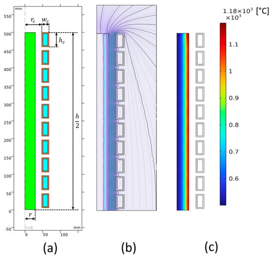
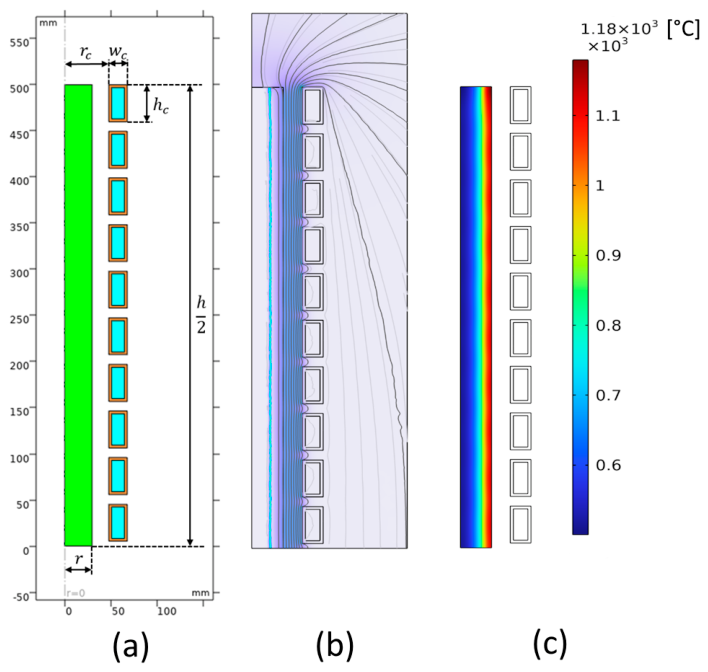
The device under consideration, as per the information provided in TEAM Workshop problem 36 [7], consists of a solenoidal inductor coil and a cylindrical steel billet, positioned coaxially with the inductor. The billet radius is r = 3 cm, the inductor has internal radius rc = 4.8 cm, its hollow turns have dimension hc by wc with hc = 4 cm and wc = 2 cm. The inductor and the billet are of equal axial length h = 100 cm: in Figure 1 half of the device is shown.
Figure 1.
Geometry of the system (a), magnetic field map (b), thermal map (c) at t = 23.1 s, I = 6 kA, f = 6 kHz.
The inductor winding comprises 20 hollow circular turns, constructed of copper conductors, connected in series and evenly spaced along the Z axis. Additionally, the inductor is assumed to operate at a frequency (f) ranging from 2 to 6 kHz, with a sinusoidal current (I) in the range of 2 to 6 kA, rms.
The cylindrical steel billet is composed of C45 steel, and its material properties, including specific heat capacity, thermal conductivity, electrical conductivity, and magnetic permeability, vary with temperature. In a prior publication [25], where the problem focused on identifying current and frequency to generate a specified thermal map, constant material properties were assumed below and above the Curie temperature of the workpiece (770 °C), i.e., a piecewise-linear problem was solved. However, the present study considers a fully nonlinear and coupled field problem, as proposed in the benchmark [7].
The overarching objective of the coupled field analysis is to calculate the thermal map in the longitudinal section of the billet at different time instants. For this purpose, a 2D axisymmetric Finite Element (FE) model, utilizing a licensed code [28], is employed to solve both electromagnetic (EM) and thermal (TH) problems.
The EM problem is addressed under time-harmonic conditions, while the TH problem involves transient analysis, with thermal sources generated by the power density distribution induced in the billet. The time-dependent analysis utilizes an implicit solver employing the backward differentiation formula (BDF), where an adaptive time step algorithm adjusts its duration based on error estimates of the current solution.
The classical magnetic vector potential coupled with the scalar electric potential formulation, AV, is used to solve the time-harmonic electromagnetic problem, as follows:
where j is the imaginary unit, is the material permeability, is the magnetic permeability of vacuum, is the relative magnetic permeability, is the angular frequency, σ is the electrical conductivity, and and are the phasors of the scalar electric potential and magnetic vector potential, respectively, while is the phasor of any imposed current density distribution. Notably, the distribution of the current source is computed by imposing the electric potential on the surfaces representing the coil; this way the actual current distribution is computed and a uniform current density is not considered in the problem.
The conservation of the total current density in the conducting regions is imposed as
which corresponds to set the total current to be solenoidal.
Homogeneous Neumann boundary conditions for the magnetic vector potential are set along z = 0, while homogeneous Dirichlet conditions are applied elsewhere.
The solution of a sinusoidal steady-state problem in terms of phasorial quantities requires that all the quantities are iso-frequential sinusoids. This assumption fails when the magnetic induction exhibits a nonlinear dependence from magnetic field. Usually the EM solution in a nonlinear model considers a modified BH curve calculated in order to keep energetic equivalence between the real nonlinear model and the equivalent one.
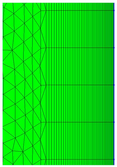
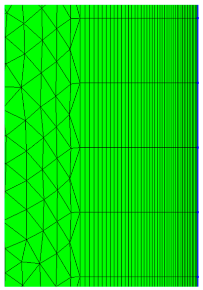
The relevant material properties in the electromagnetic solution, electrical resistivity and magnetic permeability, are both temperature dependent, while magnetic permeability also exhibits a nonlinear dependence on the magnetic field. For a given frequency, the penetration depth is minimal at cold conditions and increases by about an order of magnitude at high temperatures. To properly resolve the steep eddy current distribution, the discretization requires that at least 2 s order elements (or 4 first-order elements) are used to subdivide the outer layer of the geometric region where eddy currents occur. For this reason, the outer layer of the billet has been meshed with quadrilateral elements whose dimension increases from the surface towards the inner part, as shown in Figure 2.
Figure 2.
The mesh of the billet is structured in space.
The thermal problem solves the Fourier equation as follows:
where T is the temperature, is the mass density, cp is the specific heat capacity, and k is the thermal conductivity. Also, the thermal properties of the steel depend on temperature.
The coupling term between the EM solution and the thermal one is the distribution of the Joule losses, , that describe the source of the thermal field.
Given the cylindrical symmetry, the electromagnetic domain includes half of the inductor, half of the billet, and the surrounding air region. The thermal domain consists of half of the billet. Adiabatic conditions are imposed along the r-axis due to the symmetry, while thermal exchanges due to radiation and convection are specified on the lines describing the outer surfaces of the billet.
The model is employed to generate a database of solutions, with 40,344 finite-element solutions calculated by varying current and frequency within the defined ranges. The transient thermal analysis employs a variable time step technique. The database is populated with a constant number of transient solutions, selected based on a constant increase in the numbering of time steps. This results in denser solutions when the automatic algorithm reduces the time step duration to correctly capture the Curie’s transition, leading to several solutions when the billet surface reaches the Curie’s point.
By coupling magnetic and thermal analyses, this model addresses the forward field problem, determining the temperature map in the billet at a given time instant, considering a specific current, frequency, and time point.
2.2. Construction of the Database
A transient study was performed for each combination of input frequency and current. The duration of the transient solution can be set by two different criteria, like keeping the duration constant for each test or applying a stop criterium based on the actual temperature. To build this database, the transient solution was interrupted once the maximum temperature on the billet reached 1200 °C, by means of a stop condition defined in the solver options. Thus, the final time-instant was different for each combination. Nevertheless, this choice allows for a more practical heating process, since some combinations of input parameters may lead to very fast or very slow temperature evolutions. Temperature maps sampled on a regularly spaced grid of points and probe measurements were stored at relevant time-instants for each case, thus preserving the knowledge of the transient evolution of temperature for any particular combination.
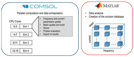
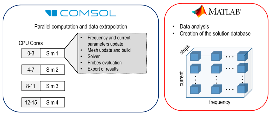
Three different workstations characterized by 2x Intel Xeon E5-2620 v4 processors (2.10 GHz, 16 cores, 32 threads) and 256 GB of RAM were used for the calculation. To exploit the full computational power, 4 parallel simulations were performed simultaneously using 4 cores each, as shown in Figure 3.
Figure 3.
Schematic of the database construction process.
At the end of each simulation, results were automatically exported and stored in .txt files using progressive notations for the filenames.
A MATLAB script was then developed to gather results from all exported files and assemble the full database, consisting of the following:
- a 5D tensor of size [Ncurr × Nfreq × Nr × Nz × nt] containing all temperature data;
- a 4D tensor of size [Ncurr × Nfreq × Nr × q × nt] containing probes measurements;
- a 3D tensor of size [Ncurr × Nfreq × nt] containing sampled time-instants;
where Ncurr is the number of current values (Ncurr = 40 values uniformly sampled in the range 2–6 kA), Nfreq is the number of frequency values (Nfreq = 40 values uniformly sampled in the range 2–6 kHz), Nr is the number of points in the radial direction (Nr = 30 sampling points along the billet radius), Nz is the number of points in the axial direction (Nz = 60 sampling points along the billet height), nt is the number of time-instants (nt = 24 time steps), and q is the number of probes defined in the FE model.
The use of a fixed number of sampled time instants provides a uniform database structure for neural network training. However, since the total heating time varies with the current–frequency combination, this strategy may lead to a low temporal resolution of sharp transient phenomena in rapidly heated cases, particularly around the Curie transition. Although the finite element solver uses adaptive time stepping and therefore provides denser solutions during highly nonlinear phases, future developments will consider adaptive or Curie-aware sampling strategies to further improve the representation of critical transient dynamics.
The last tensor contains the time step values since they are different from case to case, as described in the following.
To establish a surrogate model driven by a Convolutional Neural Network (CNN), a series of numerically evaluated temperature maps at various time points is required. A grid of 30 × 60 regularly spaced points in the billet cross-section is considered for 25 time instants. The initial time instant (t = 0) is excluded because the temperature maps are homogeneous and equal to the initial temperature (20 °C) throughout the billet cross-section. The MATLAB script extracts 25 temperature maps from each FE solution at different time instants, selecting them by a constant increment of the numbering of the time step, without applying any interpolation of results between two time steps.
Specifically, the transient thermal solution was obtained on a very dense grid in axisymmetric 2D space discretized by second-order elements, while the time discretization, i.e., the duration of the time steps, is variable according to the algorithm used by Comsol Multiphysics solver for handling the transient problem. The calculated thermal distribution was used to train the neural network by postprocessing the solution to evaluate the temperatures on a grid of 30 × 60 = 1800 equally spaced points. Obviously, the grid of 1800 points may not overlap perfectly with the mesh, but the interpolation performed by Comsol represents a trivial data post-processing operation performed by the software.
2.3. Neural Network Training
To solve the underlying multiphysics problem, the database allows for the training of Deep Neural Networks (DNNs) in general. The focus of the article is on training a specific neural network, the Convolutional Neural Network (CNN) [20], to address the TEAM 36 problem. Temperature identification is conducted along radial lines (i.e., z = k, where 0 < k < 50 cm), computing it at 30 test points along the radial direction. The CNN, structured as outlined in Table 1 with 24 layers, is independently trained for various radial lines.
Table 1.
The proposed CNN architecture.
The trained CNN takes as input a vector of 3 values, as follows:
- current,
- frequency,
- time step
and produces 30 points as output, representing the temperature profile along a radial line. For each radial line, the temperature distribution is sampled on 30 measuring points.
In the CNN structure, 4 blocks can be highlighted. Each block is composed of a transposed convolutional layer, a convolutional layer, a batch normalization layer, and an activation function (Rectified Linear Unit ReLU function), as shown in Table 1.
The ReLU function is one of the most used activation functions for CNN because it has shown good performances in training this kind of neural networks in terms of avoiding overfitting.
The transposed convolutional layers are characterized by filters of size 5 × 5, while the number of filters varies from 4 to 512; the convolutional layers are characterized by filters of size 3 × 3, while the number of filters varies from 8 to 512, depending on the block. In the final block, a dropout layer is used and a fully connected layer followed by the output layer, which computes the half-mean-squared error, allows a vector of 30 elements to be obtained as output.
The CNN undergoes training for 500 epochs, utilizing a batch size of 512 [29].
The training employs the Adaptive Moment Estimation (ADAM) method with the following parameters:
- an initial learning rate of 10−4,
- a learning rate drop factor of 0.9,
- a learning rate drop period of 20.
The dataset of 40,344 samples is partitioned into 80% for training (32,275 samples) and 20% for validation (8069 samples). Prior to the dataset split, a random shuffle is applied to the samples.
3. Results
The trained CNN was used to solve the direct problem, i.e., given a prescribed set of input data (frequency, current, process time) the CNN has to predict the temperature distribution in the billet.
To assess the accuracy of temperature prediction, the Mean Absolute Percentage Error (MAPE) is utilized, as follows:
where Y represents the true temperature, values obtained from the Finite Element (FE) model, Ŷ signifies the temperature values predicted by the CNN, and N equals 30, denoting the number of points at which temperature is sampled along the radial line.
The global error Ma is then calculated as the average of the MAPE error for the whole validation set.
The CNN trained for the radial line z = 0 shows a Ma error of 6.68%.
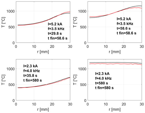
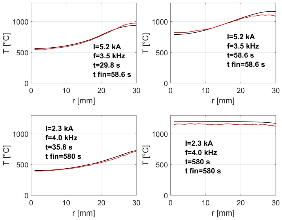
Figure 4 illustrates a comparison between temperature profiles obtained from the Finite Element Analysis (FEA) and those predicted by the CNN for selected cases. The comparisons presented here have been evaluated along the billet radius corresponding to the symmetry line, i.e., at axial position z = 0, for two different time instants of the heating process. It is underlined that the time instant, together with the frequency-current pair, is an input to the network for the estimation of the temperature profile.
Figure 4.
Temperature vs. radius: black—FEM, red—CNN prediction. Two different cases are considered, referring to two different frequency-current pairs. The temperature distribution along the radial line at z = 0 is plotted for two different time steps, at the beginning and at the end of the heating process.
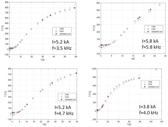
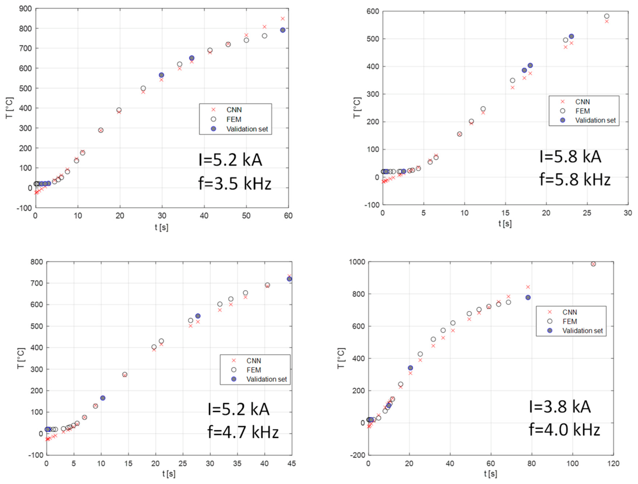
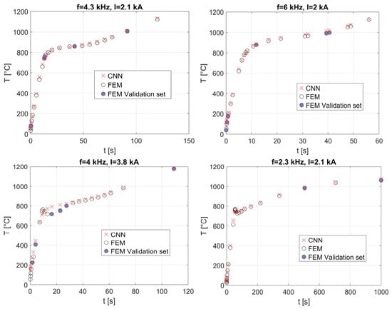
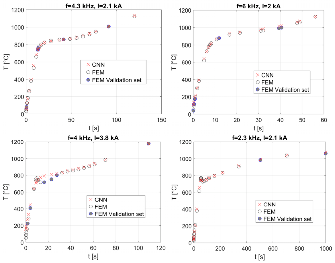
Figure 5 and Figure 6 show some temperature transients evaluated at a point on the billet surface calculated by the FE model and those obtained from the trained CNN. The trained CNN effectively predicts the temperature evolution resulting from a given set of current and frequency values for the majority of the considered time instances during the transient process, as the ones presented in Figure 5.
Figure 5.
The first part of some temperature transients evaluated at a point on the billet surface (z = 0, r = 3 cm) as calculated by the FE model and those obtained from the trained CNN. Some temperature points represented in the figure have been used in the validation set (in blue in the figure).
Figure 6.
Full temperature evolution of a point on z = 0, r = 3 cm.
There are time instants, particularly at the beginning of the process and during Curie’s transition, where the accuracy may be compromised. In fact, for certain time instants, the accuracy diminishes around the Curie temperature, as evidenced in the bottom plots of Figure 6.
Discrepancies in predicting temperature distributions at the start of the process may be attributed to the steep derivatives, both in time and space, occurring close to the billet surface. The temperature profile along the radial lines at the process start, as shown in Figure 5, exhibits a flat distribution up to the nearby surface, where it experiences a sudden increase. This abrupt temperature growth is a result of concentrated Joule losses in a penetration layer, which is small due to the magnetic nature and low electrical resistivity of the cold steel. Significant discrepancies are observed, particularly when input data fall within the range of high supply current and frequency.
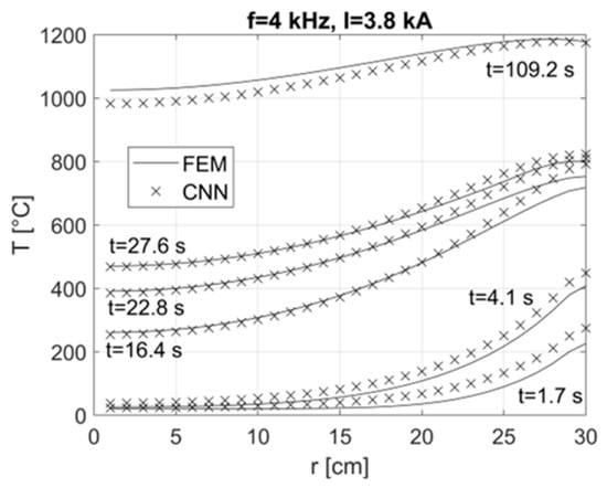
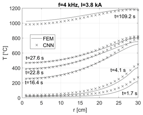
In Figure 7, a comparison between the temperature predicted by the CNN and the FEM values along the radial line z = 0 for different time instants is shown. The case f = 4 kHz and I = 3.8 kA is considered; this case is critical for the temperature prediction around the Curie point (see Figure 6).
Figure 7.
Temperature versus billet radius for different time instants of the validation set, case f = 4 kHz, I = 3.8 kA.
Figure 7 confirms that the temperature prediction is more critical for the initial time instants (see cases t = 1.7 s and t = 4.1 s) close to the billet surface and around the Curie point, close to the billet surface (see cases t = 16.4 s and t = 22.8 s), as well.
The same CNN is able to provide a stable performance in temperature reconstruction if tested for all the radial lines up to z = 39.8 cm. However, from z = 46.6 cm up to 50 cm, the error increases up to 13.7%. For these last lines, different CNNs with the same architecture are independently trained.
The results of the CNNs independently trained for the lines z = 0 and for five radial lines close to the billet end (46.6 < z < 50 cm) are shown in Table 2.
Table 2.
Global error Ma for temperature reconstruction along different radial lines.
Considering the 60 equally spaced radial lines at different z-coordinates, with 0 < z < 50 cm, 60 CNNs independently trained showed a mean and standard deviation of the Ma error equal to 8.88% and 2.1%, respectively.
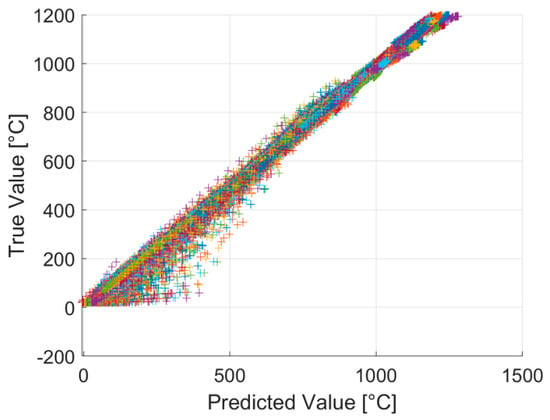
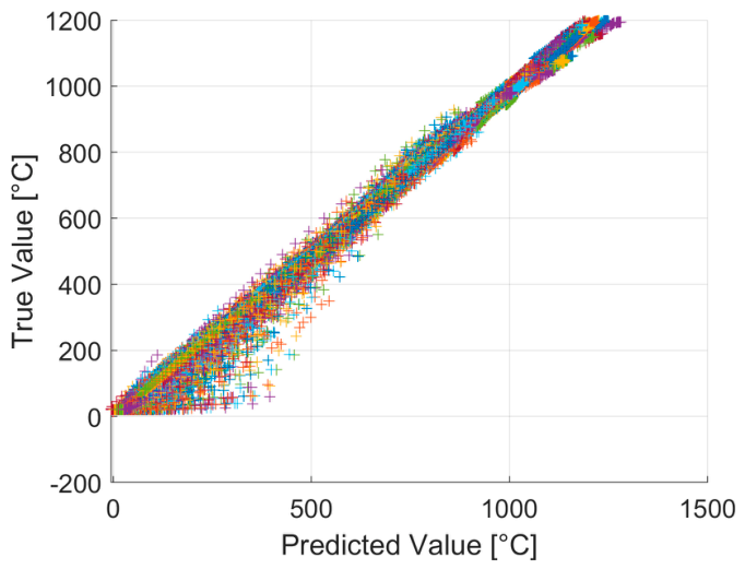
Considering the true versus predicted values plot (see Figure 8) for a line which direction crosses a turn section, i.e., z = 2.4 cm, it seems that the CNN is able to correctly predict the temperature around the Curie point. On the other hand, the initial part of the thermal time-transient seems still critical.
Figure 8.
True versus predicted values of temperature for the line z = 2.4 cm.
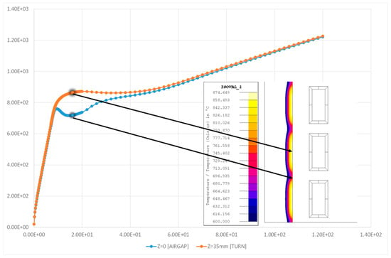
Regarding differences around Curie’s transition, the analysis reveals a more complex dependence. Discrepancies are more pronounced along lines positioned at the same height as an air gap between the inductor’s turns, while the predicted distribution closely matches the true one along lines facing a copper turn. Further investigation into this behaviour involves analysing the Finite Element Analysis (FEA) results from the database. This analysis highlights a non-monotonic growth in surface temperature over time for points positioned in front of an air gap, at least for several cases in the database set. On the contrary, temperature exhibits a monotonic growth for points at the same height as the copper turns.
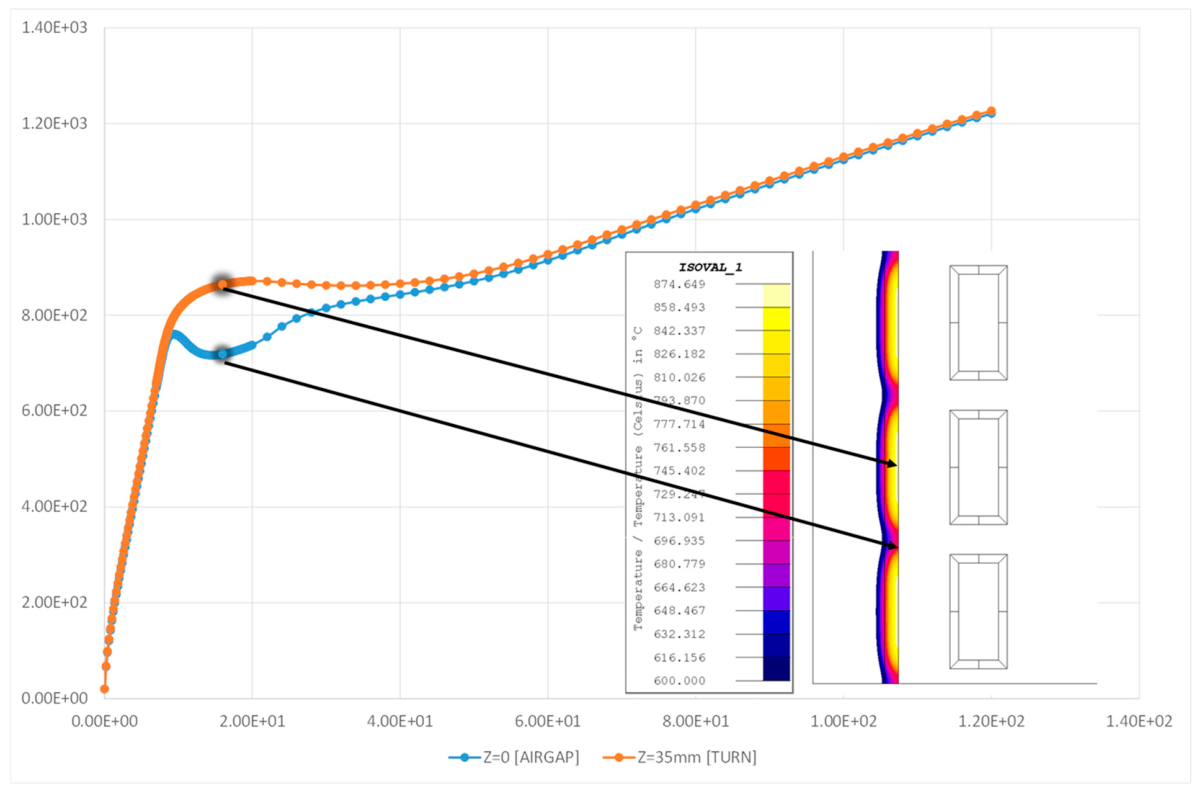
Additional numerical calculations using a different commercial FEA tool (Flux, Altair [30]) confirm this behaviour. Figure 9 presents the thermal transient [I = 3.8 kA; f = 4 kHz] of two surface points along with the colour map of temperature evaluated after 16 s, representing the instant when the model shows the most significant temperature differences. The non-monotonic growth of temperature on surface points corresponding to inter-turn positions is consistently captured by different commercial FEA tools.
Figure 9.
Thermal transient evaluated on two different surface points and the colour map describing the temperature distribution at 16 s.
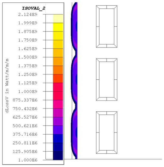
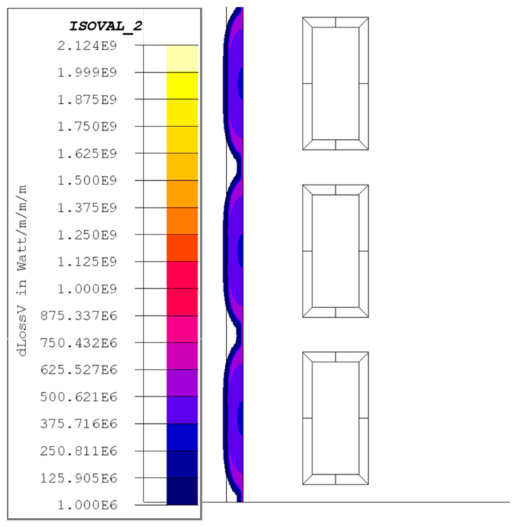
Both Finite Element (FE) analyses indicate that the inter-turn points remain below the Curie’s temperature even when the part facing the copper turn has surpassed the transition temperature on the billet surface. Consequently, the penetration depth increases in the areas in front of the inductor, allowing eddy currents to find paths of wider section and shorter length. In Figure 10, the distribution of heating sources during the Curie’s transition illustrates a decrease in the amount of heat induced in the inter-turn area, becoming lower than the corresponding heat losses due to radiation and convection. As a result, temperatures in these areas decrease until the hottest parts, those facing the inductor, transmit heat through thermal conduction. This qualitative explanation is a preliminary insight, and further numerical and experimental analyses are underway to more comprehensively understand and validate this unique effect.
Figure 10.
Distribution of Joule’s losses at time 16 s.
4. Conclusions
The CNN, trained with approximately 40,000 Finite Element Analyses (FEAs), can predict the temperature distribution along a line with acceptable accuracy. However, its performance diminishes in temperature prediction when materials exhibit nonlinear properties, especially around the Curie point, particularly for points situated along an inter-turn line. Conversely, it appears that the temperature reconstruction around the Curie point is relatively accurate for points located farther away from an inter-turn line.
The degradation of the prediction accuracy, observed in proximity of the Curie temperature and in regions aligned with the coil inter-turn gaps, can be attributed to the strongly nonlinear nature of the electromagnetic–thermal coupling, where the temperature dependence of the magnetic properties significantly affects the heat generation distribution and the subsequent thermal evolution. The proposed model is purely data-driven and does not explicitly incorporate temperature-dependent physical constraints or material laws during the training process. Therefore, further improvements could be achieved by introducing physics-informed regularization terms accounting for Curie transition effects or by using adaptive sampling strategies that increase the representation of highly nonlinear operating regimes in the training dataset. An alternative approach would be developing segmented surrogate models with dedicated models for the pre-Curie, transition, and post-Curie temperature regimes. Such strategies could improve the prediction fidelity in critical regions characterized by strong variations of electromagnetic properties and non-monotonic temperature evolution.
However, the observed nonlinearity around the Curie point, particularly for points along an inter-turn line, adds a layer of complexity to this benchmark problem, making it challenging for accurate temperature prediction in these specific scenarios.
It is worth notice that the FE model used for the database creation took into account a mapped mesh, able to properly model the Curie transition, in an adaptive way.
To best knowledge of the authors, this is the first time that a deep learning approach is applied to the forward field problem of the benchmark TEAM 36. Accordingly, having a fast model for temperature prediction in the billet puts the ground for real-time optimal control of the process, given frequency and current values. The main limitation of the proposed approach is the loss of accuracy in the inter-turn region of the billet and when working around the Curie point, which could be due to poor discretization in time. To overcome these issues, future work could include physics-informed layers and a larger database of solutions, increasing the time resolution, specifically around the Curie temperature.
Author Contributions
Conceptualization, P.D.B. and F.D.; methodology, M.F. and M.E.M.; software, M.F. and M.E.M.; validation, P.D.B. and F.D.; formal analysis, P.D.B.; investigation, M.F.; data curation, M.F.; writing—original draft preparation, M.F. and M.E.M.; writing—review and editing, P.D.B.; visualization, M.E.M.; supervision, F.D. All authors have read and agreed to the published version of the manuscript.
Funding
This research received no external funding.
Data Availability Statement
The raw data supporting the conclusions of this article will be made available by the authors on request.
Conflicts of Interest
The authors declare no conflicts of interest.
Abbreviations
The following abbreviations are used in this manuscript:
| FEA—FEM | Finite Element Analysis—Method |
| EM | Electromagnetic |
| TH | Thermal |
| CNN | Convolutional Neural Network |
| DNN | Deep Neural Network |
References
- Rudnev, V.; Loveless, D.; Cook, R.; Black, M. Handbook of Induction Heating; CRC Press: Boca Raton, FL, USA, 2017. [Google Scholar]
- Lupi, S. Induction Heating: Industrial Applications; Springer: Milan, Italy, 2014. [Google Scholar]
- Goldstein, R.J. Induction Heat Treatment of Steel; ASM International: Materials Park, OH, USA, 1999. [Google Scholar]
- Bouillault, F.; Coulomb, J.L.; Keradec, J.P. Modelling of induction heating processes: Application to axisymmetric cases. IEEE Trans. Magn. 1991, 27, 4160–4162. [Google Scholar]
- Jack, A.G.; Mecrow, B.C.; Haylock, J.A. A comparative study of finite element and equivalent circuit modelling of induction heating. IEE Proc. B Electr. Power Appl. 1990, 137, 259–268. [Google Scholar]
- Zinn, S.; Semiatin, S.L. Elements of induction heating: Design, control, and applications. ASM Handb. 1988, 4, 429–444. [Google Scholar]
- TEAM Workshop Problem 36. Testing Electromagnetic Analysis Methods (TEAM). Available online: http://www.ics.ee.ic.ac.uk/team/ (accessed on 7 April 2026).
- Bossavit, A. A rationale for edge elements in 3D field computations. IEEE Trans. Magn. 1988, 24, 74–79. [Google Scholar] [CrossRef] [Scilit]
- Chaboudez, C.; Clain, S.; Glardon, R.; Mari, D.; Rappaz, J.; Swierkosz, M. Numerical Modeling in Induction Heating for Axisymmetric Geometries. IEEE Trans. Magn. 1997, 33, 739–745. [Google Scholar] [CrossRef] [Scilit]
- Di Barba, P.; Mognaschi, M.E.; Lowther, D.A.; Dughiero, F.; Forzan, M.; Sieni, E. A Benchmark Problem of Induction Heating Analysis. Int. J. Appl. Electromagn. Mech. 2017, 53, S139–S149. [Google Scholar] [CrossRef] [Scilit]
- Di Barba, P.; Dughiero, F.; Forzan, M.; Sieni, E. New solutions to a multi-objective benchmark problem of induction heating: An application of computational biogeography and evolutionary algorithms. Arch. Electr. Eng. 2018, 67, 139–149. [Google Scholar] [CrossRef] [Scilit]
- Gong, R.; Tang, Z. Training Sample Selection Strategy Applied to CNN in Magneto-Thermal Coupled Analysis. Trans. Magn. 2021, 57, 8401104. [Google Scholar] [CrossRef] [Scilit]
- Baldan, M.; Di Barba, P.; Lowther, D.A. Physics-informed neural networks for inverse electromagnetic problems. IEEE Trans. Magn. 2023, 59, 7000904. [Google Scholar] [CrossRef] [Scilit]
- Khan, A.; Ghorbanian, V.; Lowther, D. Deep Learning for Magnetic Field Estimation. Trans. Magn. 2019, 55, 7202304. [Google Scholar] [CrossRef] [Scilit]
- Schmeing, L.; Pioch, F. Advancements in Physics-Informed Neural Networks for Solving Maxwell’s Equations: A Systematic Literature Review. Electronics 2026, 15, 2424. [Google Scholar] [CrossRef] [Scilit]
- Asadzadeh, M.Z.; Roppert, K.; Raninger, P. Material data identification in an induction hardening test rig with physics-informed neural networks. Materials 2023, 16, 5013. [Google Scholar] [CrossRef] [Scilit] [PubMed]
- Ghafoorinejad, A.; Di Barba, P.; Dughiero, F.; Forzan, M.; Mognaschi, M.E.; Sieni, E. A cascade deep learning approach for design and control optimization of a dual-frequency induction heating device. Energies 2025, 18, 6598. [Google Scholar] [CrossRef] [Scilit]
- Lahuerta, O.; Carretero, C.; Barragan, L.A.; Navarro, D.; Acero, J. Hybrid-timescale physics-informed neural network for electrical equivalent impedance identification in induction heating systems. IEEE Open J. Ind. Electron. Soc. 2026, 7, 382–392. [Google Scholar] [CrossRef] [Scilit]
- Baldan, M.; Di Barba, P. Energy-based PINNs for solving coupled field problems: Concepts and application to the multi-objective optimal design of an induction heater. IET Sci. Meas. Technol. 2024, 18, 514–523. [Google Scholar] [CrossRef] [Scilit]
- Goodfellow, I.; Bengio, Y.; Courville, A. Deep Learning; MIT Press: Cambridge, MA, USA, 2016. [Google Scholar]
- LeCun, Y.; Bengio, Y.; Hinton, G. Deep learning. Nature 2015, 521, 436–444. [Google Scholar] [CrossRef] [Scilit] [PubMed]
- Schmidhuber, J. Deep learning in neural networks: An overview. Neural Netw. 2015, 61, 85–117. [Google Scholar] [CrossRef] [Scilit] [PubMed]
- Raissi, M.; Perdikaris, P.; Karniadakis, G.E. Physics-informed neural networks: A deep learning framework for solving forward and inverse problems. J. Comput. Phys. 2019, 378, 686–707. [Google Scholar] [CrossRef] [Scilit]
- Karniadakis, G.E.; Kevrekidis, I.G.; Lu, L.; Perdikaris, P.; Wang, S.; Yang, L. Physics-informed machine learning. Nat. Rev. Phys. 2021, 3, 422–440. [Google Scholar] [CrossRef] [Scilit]
- Fawaz, H.I.; Forestier, G.; Weber, J.; Idoumghar, L.; Muller, P.-A. Deep learning for time series classification: A review. Data Min. Knowl. Discov. 2019, 33, 917–963. [Google Scholar] [CrossRef] [Scilit]
- Lim, B.; Zohren, S. Time-series forecasting with deep learning: A survey. Philos. Trans. R. Soc. A 2021, 379, 20200209. [Google Scholar] [CrossRef] [Scilit] [PubMed]
- Di Barba, P.; Mognaschi, M.E.; Cavazzini, A.M.; Ciofani, M.; Dughiero, F.; Forzan, M.; Lazzarin, M.; Marconi, A.; Lowther, D.A.; Sykulski, J.K. A numerical twin model for the coupled field analysis of TEAM Workshop Problem 36. IEEE Trans. Magn. 2023, 59, 7000904. [Google Scholar] [CrossRef] [Scilit]
- Comsol Multiphysics. Available online: https://www.comsol.com/ (accessed on 15 April 2026).
- Ioffe, S.; Szegedy, C. Batch normalization: Accelerating deep network training by reducing internal covariate shift. In Proceedings of the 32nd International Conference on Machine Learning, ICML, Lille, France, 6–11 July 2015. [Google Scholar]
- Altair Engineering. Altair Flux. Available online: https://altair.com/flux (accessed on 15 April 2026).

Disclaimer/Publisher’s Note: The statements, opinions and data contained in all publications are solely those of the individual author(s) and contributor(s) and not of MDPI and/or the editor(s). MDPI and/or the editor(s) disclaim responsibility for any injury to people or property resulting from any ideas, methods, instructions or products referred to in the content. |
© 2026 by the authors. Licensee MDPI, Basel, Switzerland. This article is an open access article distributed under the terms and conditions of the Creative Commons Attribution (CC BY) license.