WindPower-SAFusion: A Sparse-Attention and Multi-Scale Fusion Model for Wind-Power Forecasting

Abstract

Accurate wind-power forecasting is essential for grid scheduling when renewable generation becomes highly variable. This study developed WindPower-SAFusion, an Informer-inspired forecasting model designed for long wind-power sequences. The framework is built around three complementary designs. First, ProbSparse self-attention is used to lower the attention cost from $O\left(L^2\right)$ to $O\left(L\log L\right)$ while retaining informative temporal dependencies. Second, convolutional distillation is embedded in the encoder to summarize local fluctuations and form multi-scale representations. Third, historical theoretical power and wind speed are fused in a recursive forecasting scheme for multi-step prediction. The model is evaluated using measured data from the Daliang Wind Farm in Guazhou, Gansu Province, China. Experiments conducted using 1-day, 3-day, and 7-day horizons show that WindPower-SAFusion obtained lower errors and higher explanatory ability than the selected statistical and deep learning baselines. The ablation results further confirm the contributions of sparse attention, convolutional feed-forward extraction, and sequence distillation. These findings indicate that the proposed framework can provide an effective data-driven tool for wind-farm dispatching and power-management applications.

1. Introduction

Wind power has become a major source of renewable electricity as power systems move toward low-carbon operation. Its growing installed capacity and grid connection scale also make forecasting more important because wind generation is inherently intermittent and rapidly changing. Forecasting errors may disturb real-time power balance, increase the need for balancing reserves, and raise operating costs in dispatching practice [1]. For system operators, more reliable forecasts provide advance information for unit commitment, reserve allocation, frequency regulation, and curtailment control. Therefore, improving wind-power forecasting accuracy is directly related to wind-power accommodation, operational economy, and the coordinated use of peak-shaving resources [2].

Existing forecasting approaches can be roughly grouped into physical-model-based methods and data-driven methods. Physical approaches usually rely on numerical weather prediction and atmospheric dynamics to describe wind-farm meteorological conditions and then infer the corresponding power output [3]. Representative sources of meteorological prediction include the Global Forecast System and products from the European Centre for Medium-Range Weather Forecasts [4,5]. These methods are useful for horizons from several hours to several days, but their performance is strongly affected by the resolution and quality of meteorological inputs [6]. On complex terrain, local topography and small-scale turbulence may be difficult to represent, and computational costs can also be high [7]. To alleviate these limitations, recent studies have explored finer spatiotemporal descriptions, including micro-grid representations, for terrain-sensitive wind-power prediction [8].

Data-driven models learn the mapping from historical variables, such as wind speed or wind direction, to wind-power output [9]. Classical examples include autoregressive models, ARIMA, and exponential smoothing [10,11]. Although these models are simple and interpretable, they usually struggle with the nonlinear and non-stationary behavior of wind-power series. Machine learning methods, including support vector machines and random forests, have improved nonlinear fitting ability [12,13,14,15]; however, long-range temporal dependence and multi-horizon degradation remain difficult issues [16]. In recursive prediction, errors from earlier steps can be propagated to later steps, whereas direct prediction may underuse correlations among future horizons. These limitations motivate the development of sequence models that can handle both long temporal contexts and local fluctuations.

Deep neural networks have therefore become increasingly important in wind speed and wind-power forecasting. They offer flexible representation learning, but they must still cope with noisy measurements, uncertainty, and the coupling of patterns at different temporal scales [17]. In practical scheduling, point forecasts are also only one part of the decision process; uncertainty-aware prediction can better support reserve planning and risk assessment [18]. Hybrid and physics-informed neural models have also been investigated to improve physical consistency and transferability in renewable-energy forecasting [19,20].

To address the long-sequence dependency, local fluctuation, and multi-step error-accumulation problems in wind-power forecasting, this paper proposes WindPower-SAFusion, an improved Informer-based framework that combines ProbSparse attention, convolutional distillation, multivariate input fusion, and recursive multi-step prediction. Using measured data from the Daliang Wind Farm, the proposed model is evaluated under 1-day, 3-day, and 7-day forecasting horizons and compared with representative statistical and deep learning baselines.

The remainder of this paper is organized as follows. Section 2 introduces the proposed WindPower-SAFusion framework, including sparse attention, the distillation encoder, multivariate fusion, and recursive multi-step forecasting. Section 3 presents the experimental study, where comparative experiments and ablation studies were conducted based on measured data to evaluate the engineering applicability of the proposed method. Section 4 concludes the paper and discusses future research directions.

2. Materials and Methods

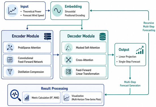
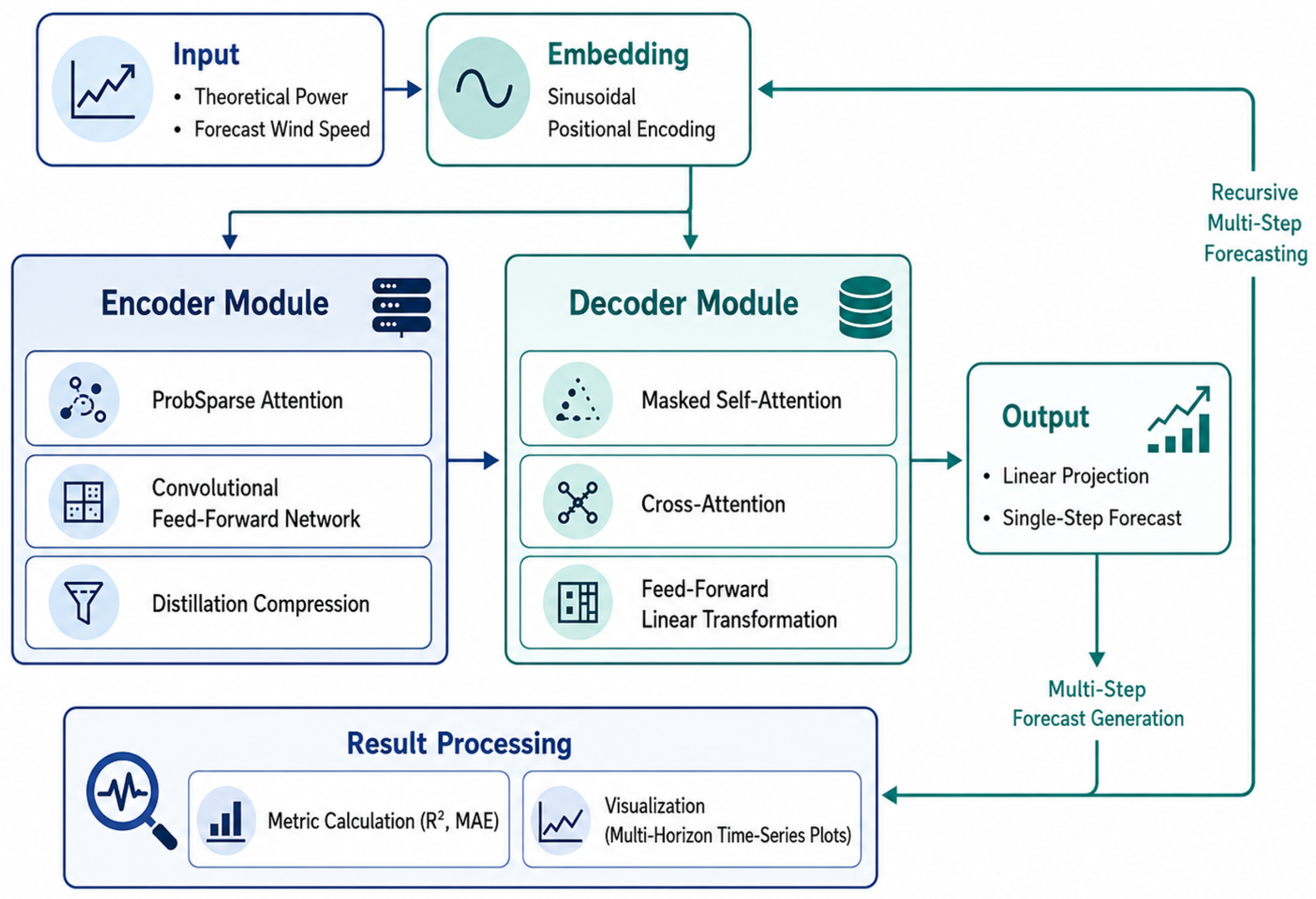
WindPower-SAFusion follows an encoder–decoder structure derived from the Informer architecture and is tailored to long wind-power sequences. Its design contains four closely connected parts: sparse attention for selecting informative time positions, convolutional distillation for local feature aggregation and sequence compression, multivariate fusion for combining historical power and wind speed, and recursive decoding for multi-step forecasting. Figure 1 summarizes the complete workflow, from input embedding and temporal encoding to decoder-based prediction and performance evaluation.

Figure 1. Overall framework of the proposed WindPower-SAFusion model.

2.1. ProbSparse Attention Mechanism

The standard Transformer computes pairwise attention among all time steps, leading to a quadratic cost with respect to sequence length [21]. This cost becomes restrictive for industrial wind-power forecasting, where the input window may be long and repeated prediction is required. To improve efficiency, WindPower-SAFusion uses the ProbSparse attention mechanism introduced by the Informer [22]. In each attention layer, the hidden sequence is projected into queries Q, keys K, and values V. A query $q_i$ represents the state of the current time step, while the key sequence $K=\{k_1,k_2,\dots ,k_{L_k}\}$ provides candidate temporal states from which information can be retrieved. The scaled dot-product scores between $q_i$ and the keys define an attention distribution over historical positions.

ProbSparse attention relies on the observation that not every query contributes equally to long-range modeling. Queries with nearly uniform attention weights provide limited information, whereas queries with one or a few dominant key responses are more likely to indicate important temporal events. These informative queries may correspond to ramp changes, abrupt fluctuations, or sustained trends in wind-power series. The following sparsity score is therefore used to rank query positions:

$$M(q_i,K)=\underset{j}{\max }\left\{{\displaystyle \frac{q_i{k}_j^T}{\sqrt{d_k}}}\right\}-{\displaystyle \frac{1}{L_k}}{\displaystyle \sum _{j=1}^{L_k}}{\displaystyle \frac{q_i{k}_j^T}{\sqrt{d_k}}},$$

(1)

where $d_k$ is the key dimension. The maximum term describes the strongest query–key response, whereas the average term gives the overall background response of the query to the key sequence. A larger value of $M(q_i,K)$ therefore means that the query has a sharper and more discriminative attention pattern. Queries with high scores are retained as dominant queries for subsequent attention computation.

In implementation, dominant connections are obtained using an approximate Top-K selection. After computing scaled dot-product scores, a mask keeps the largest responses and suppresses the remaining entries. The resulting sparse attention matrix is written as follows:

$$A_{\mathrm{sparse}}=\mathrm{softmax}\left(\mathrm{Mask}\left({\displaystyle \frac{Q{K}^T}{\sqrt{d_k}}}\right),\mathrm{TopK}\right).$$

(2)

Here, $\mathrm{TopK}$ represents the retained score indices, and $\mathrm{Mask}(·)$ assigns very small values to unselected positions before the softmax operation. Consequently, negligible attention weights are given to less useful positions. Under the ProbSparse approximation, the cost of self-attention changes from $O\left(L_q{L}_k\right)$ to $O\left(L_q\log L_k\right)$, which reduces computation for long sequences while preserving the ability to model relevant temporal dependencies [22,23].

2.2. Encoder Module Design

The encoder contains $N_e$ stacked layers. Within each layer, ProbSparse self-attention is followed by residual connection and layer normalization. A convolutional feed-forward network (Conv-FFN), a second residual-normalization step, and a distillation operation are then applied. With this order, global temporal dependencies are first extracted, and local neighboring patterns are then aggregated before the sequence is shortened. The experimental settings of $N_e$ are given in Section 3.2.

The Conv-FFN replaces the conventional position-wise feed-forward network with convolutional operations to emphasize the correlations between adjacent time steps [24]. Its formulation is given by

$$\mathrm{ConvFFN}\left(Z\right)=W_2\ast (W_1\ast Z+b_1)+b_2,$$

(3)

where ∗ denotes the one-dimensional convolution operation in the temporal dimension. The variable Z denotes the hidden feature representation obtained from the preceding ProbSparse attention block after residual connection and layer normalization. Therefore, Z already contains the long-range temporal dependency information extracted from the input sequence. The parameters $W_1$ and $W_2$ denote convolutional kernels, while $b_1$ and $b_2$ are the corresponding bias terms. These parameters are not manually specified; they are initialized together with the other network parameters and optimized through backpropagation by minimizing the mean squared error loss.

Unlike a position-wise fully connected feed-forward block, the Conv-FFN updates each temporal representation with information from nearby positions. This local receptive field is useful for wind-power data because ramps and short fluctuations often appear as local changes. The Conv-FFN therefore complements the attention block: attention emphasizes long-range dependence, while convolution strengthens short-range temporal feature extraction.

Finally, a distillation compression mechanism is introduced at the end of each encoder layer. Specifically,

$$X_{\mathrm{distill}}^{\left(j\right)}=\mathrm{ReLU}\left(\mathrm{Conv}1\mathrm{D}\right(Z^{\left(j\right)}\left)\right),$$

(4)

where $Z^{\left(j\right)}$ is the representation produced by the j-th encoder layer before compression. The convolutional kernel defines the temporal neighborhood used for aggregation, the stride determines how the convolution window moves, and padding protects boundary information. Distillation first combines nearby features and then reduces sequence length, so redundant adjacent information is removed while the main temporal pattern is retained. This process builds a hierarchical representation with a lower computational cost. The kernel size, stride, and padding used in the experiments are listed in Section 3.2.

2.3. Decoder Module Design

The decoder is designed for generative multi-step prediction and includes $N_d$ decoder layers. A layer contains masked self-attention, encoder–decoder cross-attention, a linear feed-forward transformation, residual connections, and layer normalization. The compressed historical representation from the encoder is denoted as $\mathrm{Memory}$. The selected value of $N_d$ is reported with the other hyperparameters in Section 3.2.

First, the output at the end of the encoder is used as the initial condition:

$$T_{\mathrm{start}}=\mathrm{Memory}[:,-1:,:].$$

(5)

Here, $\mathrm{Memory}[:,-1:,:]$ selects, for every sample and feature dimension, the hidden state at the last encoded time step. This vector contains the most recent context after sparse attention, convolutional aggregation, and distillation. It is therefore used to initialize the decoder because it is closest in time to the future values to be generated.

Then, the initial decoder input is constructed by repeated operations:

$$T_{\mathrm{input}}=\mathrm{Repeat}\left(T_{\mathrm{start}},{\mathrm{output}}_w\right)+PE,$$

(6)

where ${\mathrm{output}}_w$ is output-window length and $PE$ represents the positional information assigned to future positions. The operation $\mathrm{Repeat}(T_{\mathrm{start}},{\mathrm{output}}_w)$ expands the initial state along the temporal axis. When ${\mathrm{output}}_w=1$, a single future point is generated at each recursive step; for a longer output window, the repeated state provides the initial scaffold for multiple positions. Adding positional encoding enables the decoder to distinguish the order of generated states without introducing ground-truth future power values.

The first layer of the decoder adopts a masked self-attention mechanism [21], ensuring that each future position can only attend to its previous or current initialized positions. This causal constraint prevents future information leakage during sequence generation. In the encoder–decoder attention layer, the model performs deep fusion between the decoding process and the encoded historical features through

$$\mathrm{CrossAttn}=\mathrm{SparseAttn}\left(T_{\mathrm{dec}},\mathrm{Memory},\mathrm{Memory}\right).$$

(7)

where $T_{\mathrm{dec}}$ is the decoder self-attention output and serves as the query. The encoder memory is used as both a key and value, allowing each generated position to retrieve relevant historical information from the encoded wind-power and wind speed sequence. If the length of the decoder sequence differs from the memory length, linear interpolation is used for temporal alignment before cross-attention. This design connects future-position information with compressed historical context and supports recursive sequence generation.

2.4. Positional Encoding and Input Representation

Absolute positional encoding is used to retain the order of observations in the sequence:

$$PE(pos,2i)=\sin \left({\displaystyle \frac{pos}{{\mathrm{10,000}}^{2i/d_{\mathrm{model}}}}}\right),$$

(8)

$$PE(pos,2i+1)=\cos \left({\displaystyle \frac{pos}{{\mathrm{10,000}}^{2i/d_{\mathrm{model}}}}}\right).$$

(9)

where $pos$ is the discrete time index, i indicates the sinusoidal frequency component, and $d_{\mathrm{model}}$ is the embedding dimension. Even embedding dimensions use the sine function, whereas odd dimensions use the cosine function. This encoding gives each time step a position-dependent vector and enables the network to preserve temporal order.

The multivariate input is mapped to the model dimension through a linear projection:

$$X_{\mathrm{embedded}}=W_e{X}_{\mathrm{input}}+b_e,$$

(10)

where $W_e$ and $b_e$ are the trainable projection matrix and bias of the embedding layer. This layer maps the original input variables, namely, historical power and wind speed, into a common $d_{\mathrm{model}}$-dimensional latent space. The matrix’s shape is determined by the input dimension and embedding size, and the bias has the same dimensions as the embedded feature vector. Both parameters are learned jointly with the rest of the network through backpropagation rather than specified from physical prior knowledge.

The final input representation is then obtained as follows:

$$X_{\mathrm{final}}=X_{\mathrm{embedded}}\times \sqrt{d_{\mathrm{model}}}+PE.$$

(11)

This representation combines the scaled embedded variables with temporal position information and provides the input used by the subsequent attention layers.

2.5. Training and Forecasting Strategy

During the training stage, the mean squared error is used as the loss function:

$$\mathcal{L}={\displaystyle \frac{1}{N}}{\displaystyle \sum _{i=1}^N}{\left(y_i-{\widehat{y}}_i\right)}^2,$$

(12)

where $y_i$ and ${\widehat{y}}_i$ denote the observed and predicted wind-power values, respectively, and N is the number of samples.

The learning rate in the t-th training epoch, denoted as ${\eta }_t$, is dynamically adjusted using a cosine annealing strategy [25]:

$${\eta }_t={\eta }_{\min }+{\displaystyle \frac{1}{2}}\left({\eta }_{\max }-{\eta }_{\min }\right)\left[1+\cos \left({\displaystyle \frac{T_{\mathrm{cur}}}{T_{\max }}}\pi \right)\right].$$

(13)

where ${\eta }_t$ denotes the learning rate used in the t-th training epoch, ${\eta }_{\max }$ denotes the initial learning rate, ${\eta }_{\min }$ denotes the minimum learning rate after annealing, $T_{\mathrm{cur}}$ represents the current epoch index in the annealing schedule, and $T_{\max }$ denotes the maximum number of epochs used to control one cosine annealing cycle. The specific optimizer, learning-rate values, weight decay, and training epochs used in the experiments are summarized in Section 3.2.

The cosine schedule starts with a relatively large step size to support fast, early optimization and then decreases the learning rate to refine the solution. Compared with a fixed learning rate, this strategy reduces late-stage oscillation while avoiding unnecessarily slow convergence, which improves training stability.

For multi-step forecasting, a recursive strategy is adopted to generate future power sequences. At each forecasting step, the predicted wind-power value is obtained as follows:

$${\widehat{y}}_t=f\left(X_{t-\tau :t-1}\right),$$

(14)

where $X_{t-\tau :t-1}$ denotes the historical input sequence from time step $t-\tau$ to time step $t-1$, and $\tau$ represents the length of the input window. Each input vector contains the multivariate features used by the model, including historical wind-power and wind speed. The function $f(·)$ represents the nonlinear mapping learned by the proposed WindPower-SAFusion model. Specifically, $f(·)$ is obtained after training the encoder–decoder network by minimizing the mean squared error loss, where all learnable parameters are optimized through backpropagation using the Adam optimizer.

After ${\widehat{y}}_t$ is generated, the input vector for the next time step is updated as follows:

$$X_t=[{\widehat{y}}_t,\mathrm{wind}\_{\mathrm{speed}}_t].$$

(15)

The predicted wind-power value ${\widehat{y}}_t$, together with the available wind speed feature at time step t, is then appended to the input sequence for the next recursive forecasting step. By repeatedly applying this procedure, the model generates multi-step future wind-power sequences while maintaining temporal continuity.

3. Results and Discussion

3.1. Data Description

In the case study, we used operational data from the Daliang Wind Farm in Guazhou, Gansu Province, China. Measurements were recorded every 15 min from November 2022 to June 2025. The available variables include time stamps, wind speed, and theoretical power. Historical theoretical power and wind speed were used as model inputs, and future theoretical power was used as the prediction target. Other meteorological variables, such as wind direction, air temperature, pressure, and humidity, were not available in the dataset. The records were split in chronological order into training, validation, and test subsets. Missing entries were filled by forward and backward filling, and the numerical variables were standardized as follows:

$$x_{\mathrm{std}}={\displaystyle \frac{x-\mu }{\sigma }},$$

(16)

where x denotes the original value; $\mu$ and $\sigma$ denote the mean and standard deviation of the corresponding variable estimated from the training set, respectively; and $x_{\mathrm{std}}$ denotes the standardized value. The same scaling parameters were then applied to the validation and independent test sets to avoid information leakage from later periods.

3.2. Experimental Settings

To respect the temporal dependence of the wind-power series, no random shuffling was performed. The earliest 80% of the samples formed the training period, and the remaining 20% was reserved as an independent test period. The final 10% of the training period was used for validation and model selection. This chronological hold-out setting is appropriate for autoregressive time-series evaluation [26]. Each input window contained 96 observations, equivalent to 24 h at a 15 min sampling interval. The evaluated horizons were 96, 288, and 672 recursive steps, corresponding to 1 day, 3 days, and 7 days. The 3-day experiment used 288 recursive steps as the main setting, while the 1-day and 7-day experiments used the same framework with the step number changed to 96 and 672. Training was performed with float32 tensors, and wind speed and power were scaled using StandardScaler. The checkpoint with the best validation performance was used for recursive testing. Performance was measured by mean absolute error (MAE) and the coefficient of determination ($R^2$).

All experiments were implemented in Python 3.12 with PyTorch. For data processing and metric computation, we used pandas, NumPy, and scikit-learn; visualization was performed with Matplotlib. CUDA acceleration was used when available; otherwise, the code ran on the CPU. To ensure reproducibility, the random seed was fixed to 7 for NumPy, Python random, and PyTorch. Table 1 reports the architecture, optimizer, attention, distillation, and learning-rate settings used in the main implementation.

Table 1. Main implementation details and hyperparameter settings.

Item	Setting
Programming language	Python
Deep learning framework	PyTorch
Preprocessing and metrics	pandas, NumPy, scikit-learn
Input variables	Historical theoretical power and wind speed
Forecasting target	Theoretical power
Sampling interval	15 min
Input sequence length	96
Single-step decoder output length	1
Forecasting horizons evaluated	96, 288, and 672 recursive steps
Main recursive forecasting length	288 steps
Sliding-window stride	5
Input dimension	2
Model dimension $d_{\mathrm{model}}$	128
Number of attention heads	4
Encoder layers $N_e$	2
Decoder layers $N_d$	1
Feed-forward dimension	256
Conv-FFN kernel size	3
Distillation kernel/stride/padding	3/2/1
Top-K attention ratio	$L_k/4$
Dropout rate	0.1
Batch size	64
Optimizer	Adam
Initial learning rate ${\eta }_{\max }$	$1\times {10}^{-3}$
Minimum learning rate ${\eta }_{\min }$	$1\times {10}^{-5}$
Weight decay	$1\times {10}^{-5}$
Maximum epochs	50
Cosine annealing period $T_{\max }$	100
Random seed	7

3.3. Forecasting Result Analysis

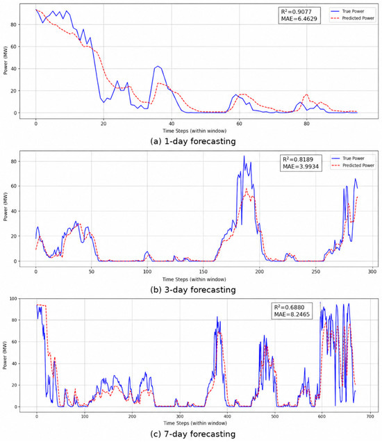
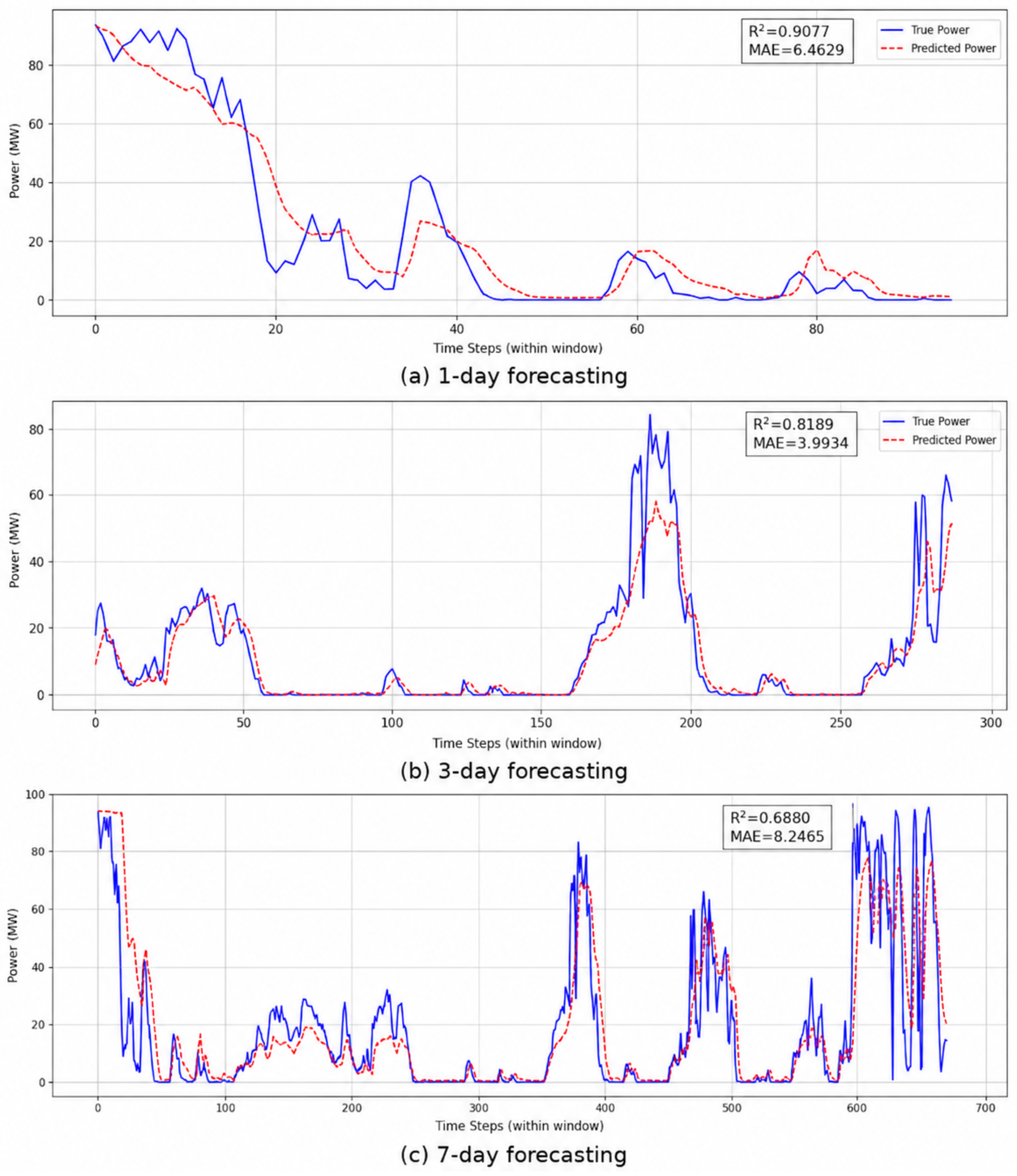
WindPower-SAFusion was examined at three horizons to assess its behavior over short, medium, and longer forecast ranges. Figure 2 shows the 1-day, 3-day, and 7-day prediction results.

Figure 2. Multi-horizon forecasting results of WindPower-SAFusion: (a) 1-day forecasting; (b) 3-day forecasting; and (c) 7-day forecasting.

For the 1-day horizon, the model obtained an $R^2$ of 0.9077 and an MAE of 6.4629 MW. The fitted curve follows the intraday variation pattern and remains responsive near abrupt changes, indicating that the sparse-attention block is able to emphasize important time positions.

For the 3-day horizon, the model reached an $R^2$ of 0.8189 and an MAE of 3.9934 MW. Although the prediction window is longer, the main trend is still well represented, and deviations can mainly be observed near several extreme values. This result shows that the distillation encoder helps combine local fluctuations with medium-range trend information.

For the 7-day horizon, the $R^2$ decreased to 0.6880 and the MAE increased to 8.2465 MW. This decline was expected because recursive prediction over a longer sequence accumulates uncertainty. Nevertheless, the predicted trajectory is broadly consistent with the observed trend, suggesting that the recursive strategy preserves temporal continuity over extended horizons.

It should be noted that the MAE of the 3-day forecast is lower than the MAE of the 1-day forecast. This phenomenon does not indicate that longer-horizon forecasting is inherently easier than short-horizon forecasting. Instead, it is mainly related to the distributional characteristics and local volatility of the corresponding evaluation samples. The 1-day forecasting window contains more abrupt short-term fluctuations and ramp-like variations, which increase the point-wise absolute prediction error. In contrast, the evaluated 3-day forecasting window is dominated by relatively smoother medium-term trend variations, which can be captured more stably by the proposed multi-scale distillation encoder and recursive forecasting strategy. Moreover, the $R^2$ value decreases from 0.9077 for the 1-day horizon to 0.8189 for the 3-day horizon, indicating that the overall explanatory ability of the model still declines as the forecasting horizon increases. Therefore, the non-monotonic change in MAE across different forecasting horizons is mainly caused by differences in local volatility and sample distribution rather than a calculation error.

Taken together, the multi-horizon results indicate that WindPower-SAFusion maintains usable forecasting ability from 1 to 7 days. Sparse attention strengthens the selection of informative temporal positions, distillation supports multi-scale representation, and multivariate input improves adaptability across horizons. Their combination leads to stable long-sequence forecasting performance.

3.4. Comparative Analysis

3.4.1. Comparison of Experimental Designs

Representative baselines were selected to provide a balanced comparison across different forecasting paradigms. The baseline set was required to include commonly used or advanced time-series methods and cover both statistical and deep learning architectures.

The comparison therefore includes N-BEATS, Temporal Fusion Transformer (TFT), TS-CNN-Attention, and ARIMA. N-BEATS uses fully connected blocks to decompose and extrapolate time-series patterns [27]. TFT combines recurrent processing, attention, and variable selection for interpretable multi-horizon forecasting [28]. TS-CNN-Attention integrates convolutional sequence extraction with attention weighting to represent local features and important temporal positions [21,24]. ARIMA is retained as a classical linear statistical baseline for time-series forecasting [11].

All methods used the same chronological data split and the same preprocessing procedure. Input variables were standardized consistently across models. The deep learning baselines were trained with the Adam optimizer and early stopping. Final performance was compared using MAE and $R^2$.

3.4.2. Comparative Experimental Result Analysis

Table 2 reports the test-set results for the four baselines and the proposed model. The reported metrics were calculated for the same complete rolling-window test period.

Table 2. Comparative of experimental results.

Model	MAE	${\mathit{R}}^2$	p-Value	Sig.
ARIMA	10.6463	0.4544	$p<0.001$	$\ast \ast \ast$
N-BEATS	7.6895	0.6464	0.0008	$\ast \ast \ast$
TFT	8.2432	0.6882	0.0011	$\ast \ast$
TCA	6.9182	0.6325	0.0006	$\ast \ast \ast$
WindPower-SAFusion	4.3478	0.8977	–	–

The (p)-values and significance labels are reported for pairwise comparisons between each baseline model and WindPower-SAFusion based on matched absolute prediction errors on the test set. Significance levels are denoted as ($\ast \ast$) for (p < 0.01) and ($\ast \ast \ast$) for (p < 0.001).

Statistical significance was assessed with a two-sided paired t-test on matched absolute errors. For each baseline, its absolute-error sequence was paired with the corresponding sequence from WindPower-SAFusion on the same test samples. The test was applied to the paired error differences, with the null hypothesis being that the two methods had equal mean absolute errors. Thus, a small p-value indicates that the observed MAE reduction is unlikely to be caused by random sample variation. Significance is denoted as ∗ for $p<0.05$, $\ast \ast$ for $p<0.01$, and $\ast \ast \ast$ for $p<0.001$.

As shown in Table 2, WindPower-SAFusion provides the lowest MAE and the highest $R^2$ among the evaluated methods. Its MAE is 4.3478, which can be compared with 10.6463 for ARIMA, 7.6895 for N-BEATS, 8.2432 for TFT, and 6.9182 for TCA. These values correspond to error reductions of 59.2%, 43.4%, 47.3%, and 37.1%, respectively. The $R^2$ value also increased to 0.8977, indicating stronger agreement with the observed wind-power sequence. The paired tests further show significant differences between WindPower-SAFusion and every baseline ($p<0.01$), supporting the reliability of the performance gain.

The advantage of WindPower-SAFusion mainly comes from the precise aggregation of key time steps by the sparse attention mechanism and the multi-scale feature extraction capability of the multi-layer distillation encoder.

(1) N-BEATS relies mainly on fully connected blocks for temporal pattern decomposition, which limits its ability to model long-sequence dependencies in highly fluctuating wind-power series.

(2) TFT combines recurrent structures, attention, and variable selection, but its representation of feature interactions may still be insufficient when the input variables are limited and the forecasting horizon becomes long.

(3) TS-CNN-Attention focuses on local temporal feature extraction and attention-based weighting; however, without the proposed sparse-attention and distillation design, its overall forecasting accuracy remains inferior to that of WindPower-SAFusion.

Overall, WindPower-SAFusion demonstrates clear advantages in forecasting accuracy, stability, and structural adaptability.

3.5. Ablation Study

3.5.1. Ablation Study Design

A controlled ablation study was conducted to isolate the contribution of the main components. Three variants were compared with the complete model. Variant A removes the Conv-FFN to test the importance of local temporal extraction. Variant B removes ProbSparse attention to examine its effect on key-time-step selection. Variant C removes the distillation mechanism to evaluate the role of sequence compression and multi-scale representation. The same MAE and $R^2$ metrics were used for all variants.

3.5.2. Ablation Study Result Analysis

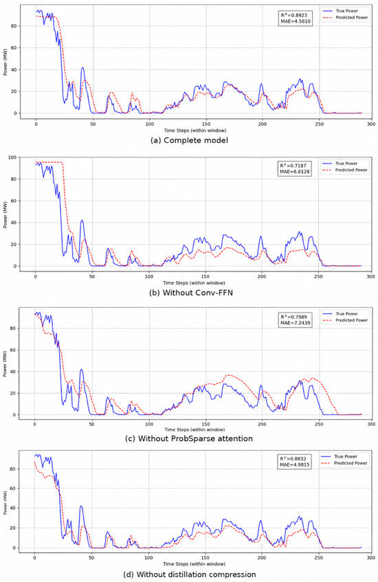
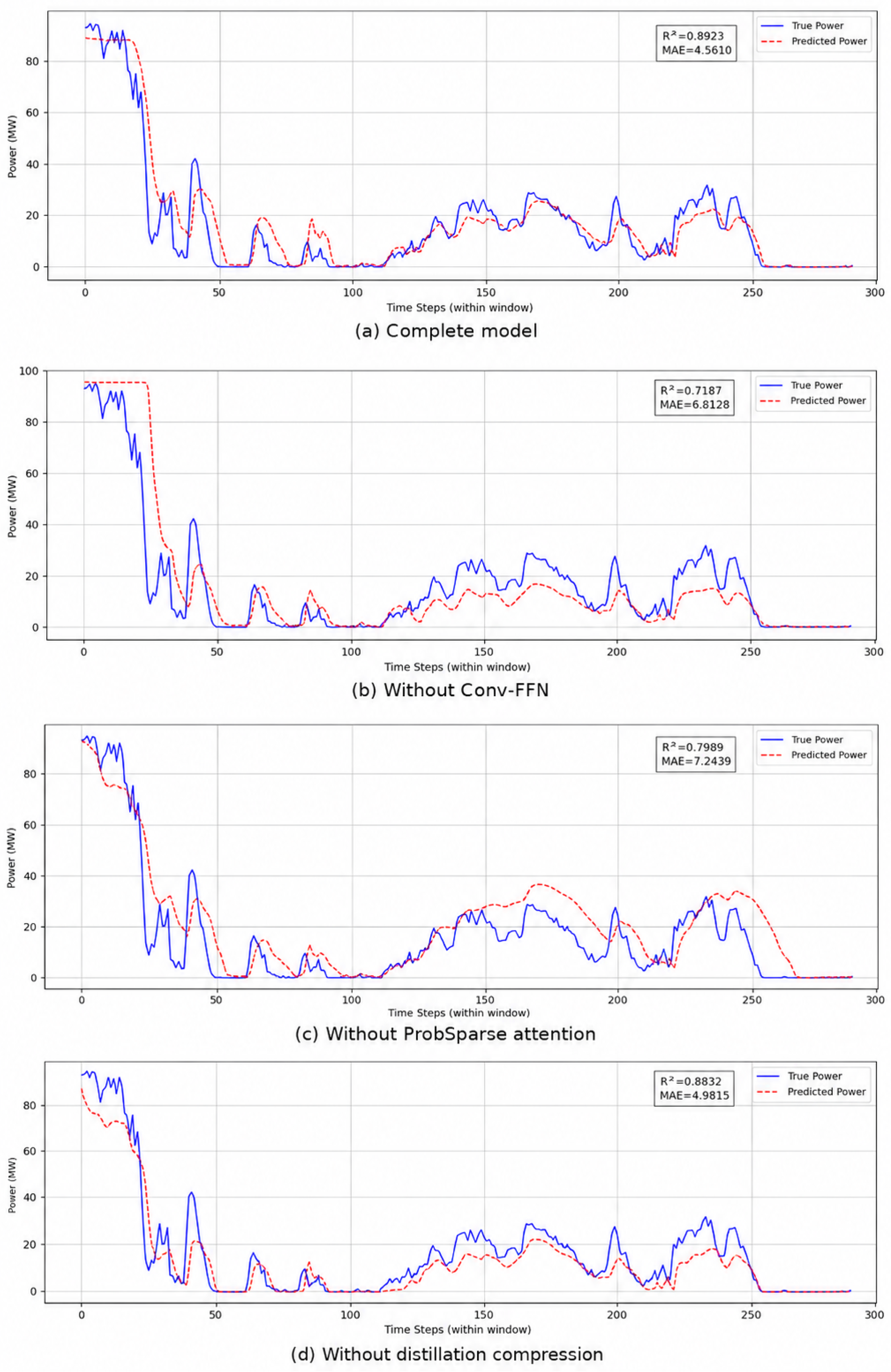
Table 3 summarizes the results for the three ablated variants. Removing any component reduces performance, indicating that the modules contribute complementary information.

Table 3. Ablation study results.

Model	MAE	${\mathit{R}}^2$
WindPower-SAFusion	4.5610	0.8923
Variant A	6.8128	0.7187
Variant B	7.2439	0.7989
Variant C	4.9815	0.8832

Variant A shows a higher MAE and a lower $R^2$ than the full model, confirming that convolutional local extraction is helpful for representing ramps and short-term fluctuations. Variant B produces the largest MAE increase, which indicates that ProbSparse attention is important for emphasizing informative time positions and reducing the influence of less useful dependencies. Variant C causes a smaller but still visible degradation, suggesting that distillation contributes to redundancy reduction, trend preservation, regularization, and computational efficiency.

These results show that the best performance is obtained when the three modules operate together. Sparse attention selects informative temporal positions, Conv-FFN captures local patterns, and distillation compresses the sequence while preserving multi-scale features. The degradation observed after removing any module supports the necessity of the integrated design.

Taking Figure 3 as an example, we used different model variants to forecast the same 3-day time period. From top to bottom, the figure presents the forecasting results of the original model, the model without the convolutional feed-forward network, the model without the ProbSparse attention mechanism, and the model without the distillation mechanism, respectively. It can be observed that the original model achieved the best fitting performance for the continuous 3-day data, with the predicted values almost overlapping the true values. After the convolutional feed-forward network is removed, the overall predicted values become lower, and the fitting performance decreases significantly. When the ProbSparse attention mechanism is removed, the predicted values show an overall upward bias, indicating that the forecasting performance is also affected. After the distillation mechanism is removed, the forecasting performance decreases slightly but not significantly. However, the model without the distillation mechanism exhibits a reduced running speed and a significantly longer running time.

Figure 3. Ablation study comparison of WindPower-SAFusion: (a) complete model; (b) Variant A without Conv-FFN; (c) Variant B without ProbSparse attention; and (d) Variant C without distillation compression.

3.6. Evaluation of Practical Application Value

From an engineering perspective, WindPower-SAFusion addresses several forecasting needs of wind-farm operation. Short-horizon results can assist power control and market-related decisions, medium-horizon results can support generation planning and maintenance scheduling, and longer-horizon forecasts can provide trend information for risk assessment. By reducing the mismatch between scheduled and actual generation, the model may help operators allocate reserves, frequency-regulation capacity, and peak-shaving resources more accurately. Relative to the strongest baseline, the proposed model lowers MAE by about 2.57 MW, suggesting potential benefits for imbalance-cost reduction and wind-power accommodation.

The model does not change the mechanical conversion efficiency of turbines. Its contribution is instead operational: better forecasts can support dispatching, reduce overly conservative curtailment, and improve the use of available wind energy under variable weather conditions. At the same time, sparse attention and distillation help control computational cost. The combination of forecasting accuracy and efficiency makes WindPower-SAFusion suitable for practical wind-power forecasting deployment.

4. Conclusions

This study presents WindPower-SAFusion for long-sequence wind-power forecasting. The model uses ProbSparse attention to reduce the cost of modeling long temporal contexts, a convolutional distillation encoder to capture multi-scale temporal features, and multivariate fusion to combine historical power with wind speed. These components jointly improve forecasting efficiency and accuracy.

The experiments show that WindPower-SAFusion outperforms the selected baselines for 1-day, 3-day, and 7-day forecasting. The ablation study further verifies that sparse attention, convolutional local extraction, and distillation each improve the final result. The model is particularly useful for sequences containing rapid changes and multi-scale variation patterns.

The present evaluation is based on measured data from a single wind farm. Therefore, additional validation is still needed for other sites, terrain types, and offshore wind scenarios. Future research will focus on lightweight model design, edge-device deployment, and transfer learning across onshore and offshore wind farms. Such extensions are expected to improve the practical usability of WindPower-SAFusion in dispatching and operation management.

References

- Zhang, B.; Chen, J.; Wu, W. Review of key technologies for large-scale wind power integration into power systems. Autom. Electr. Power Syst. 2019, 43, 2–15. [Google Scholar] [CrossRef]
- Lee, K.; Park, B.; Kim, J.; Hong, J. Day-ahead wind power forecasting based on feature extraction integrating vertical layer wind characteristics in complex terrain. Energy 2024, 288, 129713. [Google Scholar] [CrossRef] [Scilit]
- Zhao, P.; Wang, J.; Xia, J.; Dai, Y.; Sheng, Y.; Yue, J. Performance evaluation and accuracy enhancement of a day-ahead wind power forecasting system in China. Renew. Energy 2012, 43, 234–241. [Google Scholar] [CrossRef] [Scilit]
- Alessandrini, S.; Sperati, S.; Pinson, P. A comparison between the ECMWF and COSMO Ensemble Prediction Systems applied to short-term wind power forecasting on real data. Appl. Energy 2013, 107, 271–280. [Google Scholar] [CrossRef] [Scilit]
- Ignatev, E.; Deriugina, G.; Suslov, K.; Balaban, G. Development of a hybrid model for medium-term wind farm power output forecasting. Renew. Energy 2025, 249, 123200. [Google Scholar] [CrossRef] [Scilit]
- Peña, A.; Mirocha, J.D. One-year-long turbulence measurements and modeling using large-eddy simulation domains in the Weather Research and Forecasting model. Appl. Energy 2024, 363, 123069. [Google Scholar] [CrossRef] [Scilit]
- Cheng, R.; Yang, D.; Liu, D.; Zhang, G. A reconstruction-based secondary decomposition-ensemble framework for wind power forecasting. Energy 2024, 308, 132895. [Google Scholar] [CrossRef] [Scilit]
- Chen, Y.; Lin, C.; Zhang, Y.; Liu, J.; Yu, D. Proactive failure warning for wind power forecast models based on volatility indicators analysis. Energy 2024, 305, 132310. [Google Scholar] [CrossRef] [Scilit]
- Malhan, P.; Mittal, M. A novel ensemble model for long-term forecasting of wind and hydro power generation. Energy Convers. Manag. 2022, 251, 114983. [Google Scholar] [CrossRef] [Scilit]
- Cadenas, E.; Jaramillo, O.A.; Rivera, W. Analysis and forecasting of wind velocity in Chetumal, Quintana Roo, using the single exponential smoothing method. Renew. Energy 2010, 35, 925–930. [Google Scholar] [CrossRef] [Scilit]
- Box, G.E.P.; Jenkins, G.M.; Reinsel, G.C.; Ljung, G.M. Time Series Analysis: Forecasting and Control, 5th ed.; John Wiley & Sons: New York, NY, USA, 2015; pp. 12–45. [Google Scholar]
- Cortes, C.; Vapnik, V. Support-vector networks. Mach. Learn. 1995, 20, 273–297. [Google Scholar] [CrossRef] [Scilit]
- Wu, Q.; Peng, C. A least squares support vector machine optimized by cloud-based evolutionary algorithm for wind power generation prediction. Energies 2016, 9, 585. [Google Scholar] [CrossRef] [Scilit]
- Tu, C.S.; Hong, C.M.; Huang, H.S.; Chen, C.H. Short term wind power prediction based on data regression and enhanced support vector machine. Energies 2020, 13, 6319. [Google Scholar] [CrossRef] [Scilit]
- Jamii, J.; Trabelsi, M.; Mansouri, M.; Kouadri, A.; Mimouni, M.F.; Nounou, M. Medium-term wind power forecasting using reduced principal component analysis based random forest model. Wind Eng. 2024, 48, 597–616. [Google Scholar] [CrossRef] [Scilit]
- Jursa, R.; Rohrig, K. Short-term wind power forecasting using evolutionary algorithms for the automated specification of artificial intelligence models. Int. J. Forecast. 2008, 24, 694–709. [Google Scholar] [CrossRef] [Scilit]
- Liu, H.; Zhang, Z. Development and trending of deep learning methods for wind power predictions. Artif. Intell. Rev. 2024, 57, 112. [Google Scholar] [CrossRef] [Scilit]
- Pinson, P. Wind energy: Forecasting challenges for its operational management. Stat. Sci. 2013, 28, 564–585. [Google Scholar] [CrossRef] [Scilit]
- Raissi, M.; Perdikaris, P.; Karniadakis, G.E. Physics-informed neural networks: A deep learning framework for solving forward and inverse problems involving nonlinear partial differential equations. J. Comput. Phys. 2019, 378, 686–707. [Google Scholar] [CrossRef] [Scilit]
- Michalakopoulos, V.; Zakynthinos, A.; Sarmas, E.; Marinakis, V.; Askounis, D. Hybrid short-term wind power forecasting model using theoretical power curves and temporal fusion transformers. Renew. Energy 2026, 256, 124008. [Google Scholar] [CrossRef] [Scilit]
- Vaswani, A.; Shazeer, N.; Parmar, N.; Uszkoreit, J.; Jones, L.; Gomez, A.N.; Kaiser, Ł.; Polosukhin, I. Attention is all you need. In Advances in Neural Information Processing Systems; Curran Associates Inc.: Red Hook, NY, USA, 2017; Volume 30, pp. 5998–6008. [Google Scholar]
- Zhou, H.; Zhang, S.; Peng, J.; Zhang, S.; Li, J.; Xiong, H.; Zhang, W. Informer: Beyond efficient transformer for long sequence time-series forecasting. In Proceedings of the AAAI Conference on Artificial Intelligence, Online, 2–9 February 2021; AAAI Press: Menlo Park, CA, USA, 2021; Volume 35, pp. 11106–11115. [Google Scholar] [CrossRef] [Scilit]
- Zaheer, M.; Guruganesh, G.; Dubey, A.; Ainslie, J.; Alberti, C.; Ontañón, S.; Pham, P.; Ravula, A.; Wang, Q.; Yang, L.; et al. Big Bird: Transformers for longer sequences. In Advances in Neural Information Processing Systems; Curran Associates Inc.: Red Hook, NY, USA, 2020; Volume 33, pp. 17283–17297. [Google Scholar]
- Dauphin, Y.N.; Fan, A.; Auli, M.; Grangier, D. Language modeling with gated convolutional networks. In Proceedings of the 34th International Conference on Machine Learning, Sydney, Australia, 6–11 August 2017; PMLR: Cambridge, MA, USA, 2017; Volume 70, pp. 933–941. [Google Scholar]
- Loshchilov, I.; Hutter, F. SGDR: Stochastic gradient descent with warm restarts. In Proceedings of the International Conference on Learning Representations, Toulon, France, 24–26 April 2017. [Google Scholar]
- Bergmeir, C.; Hyndman, R.J.; Koo, B. A note on the validity of cross-validation for evaluating autoregressive time series prediction. Comput. Stat. Data Anal. 2018, 120, 70–83. [Google Scholar] [CrossRef] [Scilit]
- Oreshkin, B.N.; Carpov, D.; Chapados, N.; Bengio, Y. N-BEATS: Neural basis expansion analysis for interpretable time series forecasting. In Proceedings of the International Conference on Learning Representations, Addis Ababa, Ethiopia, 26–30 April 2020. [Google Scholar]
- Lim, B.; Arik, S.O.; Loeff, N.; Pfister, T. Temporal Fusion Transformers for interpretable multi-horizon time series forecasting. Int. J. Forecast. 2021, 37, 1748–1764. [Google Scholar] [CrossRef] [Scilit]
Disclaimer/Publisher’s Note: The statements, opinions and data contained in all publications are solely those of the individual author(s) and contributor(s) and not of MDPI and/or the editor(s). MDPI and/or the editor(s) disclaim responsibility for any injury to people or property resulting from any ideas, methods, instructions or products referred to in the content. |
© 2026 by the authors. Licensee MDPI, Basel, Switzerland. This article is an open access article distributed under the terms and conditions of the Creative Commons Attribution (CC BY) license.