


Abstract
This article proposes a gas-only continuation framework for steady-state loadability analysis in natural gas transmission networks based on a direction-free reformulation of the General Flow Equation (GFE). The proposed formulation introduces signed pipe flows directly as state variables, thereby representing bidirectionality intrinsically. As a result, flow reversals are handled without switching logic, while the branch geometry and criticality mechanism of the underlying gas-network equilibrium map are preserved. On this basis, a Gas Continuation Method (GCM) is developed to trace equilibrium branches directly in native gas-load space under specified gas-load stress. The method distinguishes the last admissible operating point from the mathematical critical point and incorporates a formal diagnosis to determine whether the detected limiting condition is consistent with a Saddle-Node Bifurcation (SNB). The proposed framework is validated on a three-node benchmark, a realistic Belgian gas transmission network, and a 40-node test system. The results show accurate agreement with Newton–Raphson (NR) solutions in the regular operating regime, robust branch tracing near limiting conditions where standalone NR loses convergence, and consistent handling of signed pipe flows under load-induced flow reversal and under algebraic orientations assigned a priori opposite to the solved physical flow. The Belgian and 40-node cases further show that the operational admissibility limit may precede the mathematical critical point, so pressure-based feasibility and branch-level criticality emerge as related but distinct notions. These features make the proposed methodology a rigorous and practical tool for identifying admissibility limits, interpreting critical behavior, and assessing loadability margins in gas transmission networks.
1. Introduction
Natural gas transmission systems play a central role in modern energy infrastructures by supplying residential, industrial, and power-generation demands through geographically extended pipeline networks [1]. As gas and power infrastructures become increasingly coupled, understanding how these networks behave under stressed operating conditions becomes essential not only for routine operation, but also for identifying operational margins and the mechanisms that limit system performance [2,3,4,5]. For this reason, steady-state analysis remains a fundamental tool for network operation, planning, and security assessment under different operating conditions [6].
The steady-state behavior of gas transmission networks has been studied mainly from the perspectives of simulation, optimization, and capacity assessment. Recent works have addressed the solution of the steady-state gas-flow equations, compressor operation, linepack-aware planning, and the development of computationally efficient models for optimization [7,8,9], while others have examined the problem from a more rigorous mathematical standpoint, clarifying its structure, solvability, and numerical treatment [10,11].
Despite these advances, the representation of bidirectional flow remains a persistent difficulty in steady-state gas-flow modeling, since conventional direction-dependent forms of the General Flow Equation (GFE) become nonsmooth at flow reversals and may even be discontinuous. In [7], this issue is treated within an optimization framework in which integer variables are associated with flow direction and fixed from a preceding static optimization in order to reduce computational burden. In [12], directional switching in the Weymouth equation is represented through binary-behaving continuous variables within a mathematical program with complementarity constraints. Similarly, in [13], flow directions are not assumed a priori, but bidirectionality is still handled through direction-dependent concentration constraints reformulated by means of integer, nonsmooth, or complementarity-based models.
Alternative treatments of bidirectionality have also been reported. Although [14] considers a quasi-dynamic setting, it remains relevant here because bidirectional pipeline flows are captured through polyhedral McCormick-type relaxations of the Weymouth equation, while compressor operating modes are represented by continuous convex relaxations rather than mixed-integer switching. A signed steady-state pipe-flow representation is also adopted in [11,15]; however, in the former, some active elements, such as flow regulators and compressors, are still governed by explicitly directed logic that prevents reverse flow, whereas in the latter, the flow is decomposed into positive and negative components and a binary variable enforces a single active direction in each pipeline and time period. Taken together, these works show that bidirectionality is still commonly managed through auxiliary directional mechanisms, rather than being embedded intrinsically in the constitutive model.
A complementary line of research has shifted the focus from pointwise analysis toward geometric descriptions of operational limits. In this context, gas transmission capability has evolved from a single scalar limit to curve-based representations [2], while loadability and security regions have been developed in [16,17,18,19]. These approaches are valuable because they provide a geometric view of admissible operation and support fast online security assessment. However, they define admissible operating sets by requiring the equilibrium equations and operating-security constraints to hold, rather than by tracing critical branch points along a specified gas-loading path. In addition, bidirectionality is typically neglected, assumed fixed, or treated through explicit directional logic tied to an imposed flow orientation, so its fully intrinsic representation remains unresolved.
Within this line of research, ref. [20] studies gas-pressure loadability through a continuation multi-energy flow framework driven by a specified scheduling direction of natural-gas-fired generator units (NGUs). The resulting pressure curves are therefore projections of a coupled continuation path in NGU injection space, rather than gas-only branches traced in native gas-load space. Moreover, although the gas-flow equations are included in the steady-state multi-energy model, the continuation formulation itself is written only in terms of voltage magnitudes, voltage angles, and gas pressures. Consequently, bidirectionality is not represented intrinsically by signed pipe-flow state variables, but is recovered through a sign function tied to the ordering of end-node pressures. These features show that, even in a continuation-based setting, the gas-side branch is not traced directly from a gas-network equilibrium model with intrinsically embedded bidirectionality.
Motivated by the limitations identified above, the present work adopts a direction-free reformulation of the steady-state GFE. The resulting reformulation introduces pipeline flows directly as signed state variables, allowing bidirectionality to be embedded intrinsically in the equilibrium model, so that the same constitutive relation remains valid through flow reversals without external switching rules or alternative expressions. This regularity is essential for Jacobian-based analysis and singularity assessment, because it provides a gas-flow relation that remains continuous and differentiable even in the neighborhood of critical branch points.
Based on this direction-free reformulation, a Gas Continuation Method (GCM) is developed to trace steady-state gas-network equilibrium branches directly in native gas-load space under a specified gas-load stress. It is designed to preserve the intrinsic structure of the equilibrium map, including its branch geometry and criticality mechanism. Bidirectionality is represented intrinsically by incorporating signed pipe flows directly into the state vector, without pressure-dependent switching logic. The proposed method identifies both the admissibility limit, which marks the boundary of physically admissible operation, and the critical point, which is determined from the loss of regularity of the gas Jacobian. A formal diagnostic procedure is then applied to assess whether the detected critical condition corresponds to a saddle-node bifurcation (SNB).
The main contributions of this work are summarized below.
- A direction-free steady-state equilibrium formulation of the GFE is established by introducing signed pipe-flow variables directly into the state vector. This makes bidirectional operation and flow reversal intrinsic to the model without auxiliary directional variables or switching logic.
- A gas-only continuation method is developed to trace equilibrium branches directly in native gas-load space. This allows the loadability path to be followed beyond isolated Newton–Raphson solutions and provides a branch-level view of limiting behavior.
- A clear distinction between operational admissibility and mathematical criticality is introduced. The former is determined by pressure constraints and admissible operating limits, whereas the latter is associated with loss of regularity along the traced equilibrium branch.
- A local critical-point diagnostic is incorporated to assess whether the detected limiting condition is consistent with an SNB, avoiding the interpretation of criticality solely from Newton–Raphson failure or from a small conditioning indicator.
These contributions are evaluated on a three-node benchmark, a realistic Belgian gas transmission network, and a 40-node test system, which together provide a transparent validation setting, an engineering-scale transmission case, and a larger benchmark with multiple sources, loads, compressors, and signed-flow orientation effects.
The rest of the paper is organized as follows. Section 2 presents the steady-state equilibrium framework and the direction-free reformulation of the GFE. Section 3 develops the proposed GCM, including the branch-tracing procedure and the critical-point indicators. Section 4 provides the numerical validation and results for the three-node gas system, the Belgian gas transmission network, and the 40-node test system. Finally, Section 5 summarizes the main conclusions of this work.
2. Steady-State Equilibrium Framework and Direction-Free Gas-Flow Model
This section establishes the steady-state equilibrium framework adopted for the gas network under a specified loading parameter. Throughout this work, all pressure inputs are specified in gauge units and converted internally to absolute values before they enter the equilibrium equations. The conversion is , with . Hence, corresponds to atmospheric pressure, while the physical lower bound corresponds to . The same conversion is applied to operational pressure thresholds, whereas the pressures reported in the Results section are expressed in gauge units for operational interpretation. Under this convention, the analysis starts from the implicit steady-state manifold defined by
where collects the gas-network state variables, and is a scalar stress parameter that modifies a specified subset of gas demands while keeping the slack-node pressure fixed.
At this point, the main requirement is not only to state the equilibrium model, but to ensure that the map in Equation (1) has the regularity needed by the continuation procedure developed later. However, as discussed in the previous section, many steady-state gas-flow formulations determine the flow direction through explicit switching rules tied to the ordering of the end-node pressures, thereby introducing nonsmooth switching surfaces that may render tangent prediction ill-defined at flow reversals. Since the continuation and singularity assessment adopted in this work rely on the Jacobian and on the regularity of the equilibrium map, the steady-state GFE is written in a direction-free form, as presented below, in which each oriented pipe flow is represented by a signed variable.
2.1. GFE Direction-Free Reformulation
In the formulation proposed in this work, the gas is represented as a homogeneous bulk fluid through lumped thermophysical parameters rather than through an explicit multicomponent composition model. The steady-state pipeline-flow model is assumed to be isothermal; therefore, a uniform gas temperature is used in the GFE coefficients throughout the network. In addition, the compressibility factor z and the Darcy friction factor are treated as constants. These assumptions are adopted deliberately to focus the analysis on the nonlinear pressure–flow coupling of the equilibrium equations without introducing additional nonlinearities associated with thermal variations, state-dependent compressibility, or friction correlations affected by the flow regime and pipe-wall roughness. Within the same single-phase modeling level, changes in gas composition can be represented by updating the corresponding bulk thermophysical parameters or by introducing smooth composition-dependent correlations in the pipe coefficient. In contrast, two-phase flow is outside the scope of the present GFE-based formulation and would require a different constitutive residual; the continuation framework could then be applied only after the corresponding multiphase equilibrium map and its regularity properties are defined. Under these assumptions, the steady-state pipe relation is then introduced from the GFE [6].
Consider a pipe connecting nodes k and m. Let and denote the corresponding nodal pressures, and let denote the average volumetric flow. The baseline GFE for a fixed orientation is written as [6]
where , , , and G are listed in the nomenclature with their specified values. Furthermore, under the isothermal assumption, the gas temperature is uniform throughout the network, so that and, consequently, for every pipe. Hence, under the fixed orientation, the magnitude form in Equation (2) is real-valued when . For simplicity, it is defined as to omit the superscript hereafter. Accordingly, define
such that Equation (2) can be rewritten as
In practice, this relation is often paired with an explicit direction selection through the sign variable , which switches when changes sign. To incorporate this direction selection into the GFE while retaining a compact expression valid for both pressure orderings, the squared-pressure drop is defined as
such that the resulting signed form is
Note that, from Equation (6), the resulting mapping is piecewise-defined and nonsmooth on the switching surface , which corresponds to flow reversal.
Building on this observation, predictor–corrector continuation requires the equilibrium map to be locally differentiable along the continuation path. This condition ensures a unique Jacobian-based linearization and a well-defined tangent direction. At , the sign-based switch makes the local linearization non-unique and the tangent predictor ill-posed, so the traced path can exhibit regime-induced discontinuities that are artifacts of the formulation rather than intrinsic features of the equilibrium manifold. To eliminate explicit direction switching, the oriented pipe flow is introduced as a signed state variable under the fixed orientation . The constitutive relation is then rewritten so that direction is captured implicitly, yielding a mapping that is continuous and with respect to , including at .
The direction-free equation is obtained from an algebraic manipulation of Equation (6), as described below. Since and during physical operation,
and taking the absolute value of Equation (6) yields
It is worth noting that Equations (8) and (6) hold simultaneously on the solution set, and therefore can be multiplied to eliminate the square root and the explicit sign factor, yielding Equation (9).
Now, using with and Equation (7), it follows that , leading to
Equation (10) represents the direction-free gas flow equation. It is evident that, in the signed form from Equation (6), direction is enforced explicitly through , whereas in Equation (10) direction is encoded implicitly by the signed flow variable , since changes sign with , while preserving the same pressure–flow relation. Moreover, the map is with the derivative
so the Jacobian with respect to the flow variable is well-defined, including at where the derivative is 0. Since is smooth in , the resulting constitutive residual is differentiable with respect to in a neighborhood of flow reversal.
At an exact zero-flow condition, gives , and Equation (10) reduces to . Hence, the corresponding steady-state value of the oriented signed pipe-flow variable is . This condition does not imply that the whole network is inactive; rather, it represents an individual pipe with zero net steady-state flow within an otherwise operating network. Other pipes connected to the same loop or neighborhood may still carry flow while the nodal mass-balance equations remain satisfied. Such a zero-flow pipe may arise when the endpoints of that specific branch reach equal pressure, as may occur in a balanced loop or along a flow-reversal path. Because no sign function, directional switch, square-root singularity, or division by is used in the residual form, the same algebraic equation remains valid on both sides of the reversal and at the zero-flow point itself. If a zero-flow condition coincides with a loss of rank of the full network Jacobian, this is detected as a property of the complete equilibrium map through , not as a failure of the pipe-flow representation.
It is important to mention that the novelty of the present proposal does not lie in Equation (10) as an isolated expression, but in its role within the formulation of the GCM. As shown in Section 3, this relation allows the pipeline flows to enter explicitly as state variables, so that bidirectionality is carried implicitly by the equilibrium model. This is the central novelty of the proposed framework, because it makes the gas-flow relation underlying the GCM continuous and differentiable through flow reversals, thereby providing the regularity required for the continuation analysis.
2.2. Network Representation
Consider a gas network with nodes indexed by ; pipelines indexed by , where each pipeline is associated with an ordered node pair under the chosen orientation ; and compressors indexed by , so that when . Let denote the slack node and its pressure, which is fixed and not treated as a state variable. Furthermore, let denote the set of load (withdrawal) nodes. In addition, for each node , let denote the specified gas source injection and denote the specified gas demand, where the latter is allowed to depend on the loading parameter . Further, the corresponding standard volumetric pipe flow is treated as an oriented signed quantity, where represents physical flow in the assigned direction . On this basis, let , and define the state vector as
where , , and are the vectors of nodal pressures excluding , oriented pipe flows, and compressor throughputs, respectively.
From the oriented gas transmission network, the node–pipe incidence matrix is defined entrywise by
so that gives the oriented pipe-flow contribution to the nodal balance according to the assigned orientations.
Furthermore, for each pipeline with assigned direction , consistent with Equations (3) and (5), define , and let denote the corresponding pipe coefficient. The constitutive residual associated with the direction-free gas flow equation is
The constant-coefficient form in Equation (14) corresponds to the numerical studies reported in this work, where the pipe-indexed quantities and , associated with and , are fixed to isolate the branch-tracing behavior of the proposed GCM. However, the direction-free structure itself does not require to be constant. If state-dependent or flow-dependent correlations are introduced for or , the pipe coefficient becomes state dependent and the pipe residual can be written in the generalized form
In this case, the Jacobian contains the additional derivative term associated with . Hence, the continuation and local critical-point analysis remain valid provided that the selected correlations for and are positive and sufficiently smooth in the operating region being traced. If empirical friction or compressibility correlations introduce discontinuous regime switches or nonsmooth dependencies, the resulting problem must either be regularized or treated as a piecewise-smooth continuation problem. Thus, variable z and modify the Jacobian entries but do not change the direction-free state representation, the pseudo-arclength continuation structure, or the interpretation of a rank-deficient critical point.
These componentwise relations define the pipe-residual vector
Note that if one of the pipeline endpoints coincides with the slack node, the corresponding pressure in is understood as the fixed slack pressure .
2.2.1. Compressor Equations
For each compressor , the nodes denote its suction and discharge terminals, respectively. Its oriented standard volumetric throughput is denoted by and is taken positive from suction to discharge, so that admissible operation satisfies . With this convention, and are the corresponding suction and discharge nodal pressures. Thus, assuming a fixed compression ratio , the scalar compressor-ratio residual is defined through Equation (17) [6].
These component-wise residuals define the compressor-ratio residual vector
Note that, similar to the case of the pipelines, if coincides with the slack node, the corresponding pressure in is understood as the fixed slack pressure .
On the other hand, the compressor fuel consumption is represented as an additional withdrawal at the suction node. The fuel-consumption flow is defined as a function of the compressor power consumption using the relations in [6]. First, the isentropic exponent is given by
which is applicable when G does not exceed unity. Next, define the brake-horsepower rate coefficient
where , , , and denote the gas compressibility factor at suction conditions, the suction temperature, the parasitic efficiency, and the compressor efficiency, respectively. Here, is the compressor-associated suction temperature used in the horsepower model and is not required to coincide with the standard temperature used in the GFE conversion. Hence, the compressor power consumption satisfies
The compressor gas consumption is then modeled through the specific consumption function
where , , and are the compressor gas-consumption coefficients.
Therefore, the compressor contribution to the nodal flow-balance residual is defined componentwise, for each compressor , as
with all other nodal entries equal to zero. The superscript denotes the contribution associated with compressor c, thereby distinguishing per-compressor terms before nodal aggregation, which is necessary when multiple compressors are connected to the same suction or discharge node. Thus, and are the suction- and discharge-node contributions of compressor c to the nodal flow-balance residual, and the total compressor contribution is obtained by summing these terms over .
Now, let be the vector whose entries are , . The compressor incidence matrix maps compressor throughputs into nodal-balance contributions under the suction-to-discharge orientation. Its entries are defined by
Similarly, to represent the fuel-consumption term as a withdrawal applied at the suction node, define a suction-selection matrix whose entries satisfy
With this definition, the product yields a nodal vector in which contributes only at the suction node of compressor c.
Hence, the aggregate compressor contribution to the nodal flow-balance residual is written as
Accordingly, when , the compressor-related vectors and matrices are empty, so no compressor contribution enters the nodal balance.
2.2.2. Nodal Mass Balance
For each node , the combined contribution of the specified source injection and gas demand to the nodal mass balance is represented by the nodal balance term
where the loading parameter parametrizes the specified loading scenario. Let denote the nodal vector whose entries are for all . In addition, if compressors are present and consume fuel at their suction nodes, the corresponding extra withdrawals are represented by , as defined in Section 2.2.1.
Because the slack-node balance is not imposed explicitly, the balance equations are enforced only at the remaining nodes. Instead, the slack-node balance determines the balancing slack supply required to sustain the operating point associated with . Thus, recalling that , the steady-state nodal mass balance is written as
where denotes the restriction of the enclosed nodal vector to the non-slack nodes.
With these elements in place, the baseline steady-state equilibrium map is assembled as
As a result, the Jacobian () associated with Equation (28) is well defined because no discrete switching is introduced and the direction-free term of Equation (14) is with respect to .
Finally, the smallest singular value is used as a conditioning indicator for the equilibrium map [21]. In particular, a small signals proximity to a loss of local invertibility and is therefore informative for identifying a nearby minimum-conditioning point and the associated loss of regularity along the traced branch. In the present framework, this indicator is used as a mathematical diagnostic and is interpreted separately from the operational admissibility criterion introduced in Section 3.5.
3. Gas Continuation Method
This section presents the formulation of the GCM, which constitutes the main methodological contribution of this work. The method is developed for branch-centered loadability analysis along a specified loading path. Rather than focusing on isolated stressed operating points, it traces the corresponding steady-state equilibrium branch, determines the last point satisfying the adopted operational admissibility criterion, and identifies the critical point as the fold-like point of the unconstrained branch. In this way, the proposed framework combines an operational view of loadability with a mathematical characterization of the limiting structure through a gas-only analogue of continuation power flow.
The development starts from the equilibrium manifold defined implicitly by Equation (1), with the residual-block representation given in Equation (28). In this sense, the proposed approach follows the general predictor–corrector pseudo-arclength framework widely used in electric power systems to trace steady-state solution branches near turning points [22]. Here, however, that framework is adapted directly to gas transmission systems by formulating the continuation problem in terms of the gas variables and constraints, namely, the non-slack nodal pressures, the oriented pipe flows, the compressor throughputs, and the loading parameter . On this basis, the GCM traces the equilibrium manifold as varies, while allowing both turning points in and flow reversals in to be represented without reformulating the governing equations. The formulation therefore begins by specifying how enters the steady-state gas equations and then develops a predictor–corrector pseudo-arclength scheme that remains well posed at turning points.
The following development makes this adaptation explicit in the gas variables of the model. In particular, the predictor, corrector, step-size refinement, and critical-point indicators are written in terms of the non-slack nodal pressures, signed pipe-flow variables, compressor throughputs, and the loading parameter. This is necessary because the augmented Newton system, the tangent direction, the conditioning indicators, and the SNB diagnostic depend on the structure of the gas-only residual map, and on the way, bidirectional pipe flows are embedded in the state vector. Thus, the contribution is not the isolated use of pseudo-arclength continuation, but its explicit realization on a direction-free gas-network equilibrium model that can be reproduced and applied directly to gas transmission loadability analysis.
3.1. Continuation Manifold and Tangent Equation
Recalling the state vector introduced in Equation (12), the continuation is carried out in the extended state–loading vector
Accordingly, the continuation formulation is expressed in terms of the non-slack nodal pressures, the oriented pipe flows, the compressor throughputs, and the stress parameter. The loading path is defined by assigning a nonnegative participation factor to each demand node, where denotes a nonparticipating node. Under this definition, the specified gas demand at node is written as
Hence, corresponds to the base operating point, whereas increases the specified withdrawals along the prescribed stress direction. In the numerical studies of this work, only one load is increased in each continuation run, which is represented by setting
This single-load setting is adopted to isolate the limiting behavior associated with the selected stressed node and to keep the interpretation of pressure sensitivity, branch turning, and flow reversal unambiguous. Since every oriented pipeline flow is retained as a signed state variable along the continuation branch, additional sign changes in other pipelines or multiple sign changes along the same traced branch, can be identified directly from the computed flow states when they are induced by the selected stress path. However, the systematic search for loading paths that produce multiple simultaneous or sequential flow reversals is left for future work, together with simultaneous multi-load stress directions and multiparameter loadability regions.
The continuation branch is the one-dimensional manifold implicitly defined by the equilibrium condition
At regular points of this manifold, the local tangent vector is denoted by
where the superposed dot denotes differentiation with respect to the continuation-path parameter. In this context, is no longer viewed as a fixed scalar parameter, but as a continuation variable that forms part of the extended solution vector. Therefore, is well defined and measures the rate of change of the loading level along the equilibrium branch. Thus, by differentiating along the branch, the tangent must satisfy
where . Since enters the formulation only through the stressed demand terms embedded in the nodal-balance block, has the block structure
At the initial operating point, no previously accepted continuation point is available to determine the tangent orientation. Therefore, once the base solution has been obtained, the initial direction is selected by prescribing the loading component of the tangent as , which starts the branch tracing in the direction of increasing demand. The corresponding state component is obtained from the base-point linearized equilibrium equation as
provided that is nonsingular. The initial unit tangent is then defined as
After the first corrected point is accepted, the subsequent tangents are computed using the tangent-update equation, with their orientation chosen to preserve continuity with the previously accepted tangent.
3.2. Predictor Step
Let r index the points calculated along the traced continuation branch and denote either the initial operating point from which the continuation procedure is started or, more generally, a converged point on the equilibrium branch. Furthermore, let denote the associated unit tangent. The pseudo-arclength predictor is then written as
where is the pseudo-arclength step size, while the tangent components satisfy
Therefore, in explicit gas-variable form, Equation (37) becomes
Therefore, the predictor advances the gas pressures, pipe flows, compressor throughputs, and loading parameter along the local tangent direction simultaneously.
After the corrector has converged at , the tangent required for the next continuation step is updated through
To make the variable structure of this update explicit, Equation (39) can be written as Equation (40). In this form, the superposed dot denotes differentiation with respect to the continuation-path parameter, so that the unknowns are the components of the updated tangent vector at the point indexed by . The updated tangent is then normalized, and its orientation is chosen so that . In this way, the sign ambiguity of the tangent is removed, and continuity is preserved from one continuation point to the next, so that the resulting predictor remains aligned with the same local branch direction in the extended gas-variable space.
3.3. Corrector Step
The corrector step restores the predictor to the equilibrium manifold by enforcing both the gas equilibrium equations and the pseudo-arclength constraint. To this end, define the augmented continuation function as
where the scalar pseudo-arclength constraint is given by
Accordingly, the corrected point must satisfy the augmented nonlinear system
To solve Equation (43), a Newton–Raphson correction is introduced in terms of and . Linearization of Equation (43) then yields
It is worth mentioning that denotes the current Newton iterate of the corrector, whereas is the tangent inherited from the previously accepted continuation point indexed by r and therefore remains fixed during the correction step. Now, using the partition in Equation (45), this system can be written in the block form given in Equation (46). Note that the last entry on the right-hand side, , is the scalar pseudo-arclength residual defined in Equation (42). In this form, the continuation correction is expressed directly in terms of the gas variables of the problem, namely, the non-slack nodal pressures, the oriented pipe flows, the compressor throughputs, and the loading parameter.
Since is linear in , its partial derivatives in the last row are the fixed tangent components inherited from the previously accepted continuation point, namely, , , , and .
As a result, the corrector updates all these variables simultaneously. The predictor is used as the initial Newton iterate, and each correction obtained from Equation (46) is added to the current iterate. Thus, if ℓ denotes the Newton iteration counter within the corrector step, the update is written as
where and are obtained by evaluating Equation (46) at . The iteration is initialized with and is repeated until both and satisfy the specified tolerances. Once convergence is reached, the final Newton iterate is accepted as the next continuation point .
3.4. Adaptive Step-Size Refinement near Folds
Adaptive step-size control is standard in continuation and path-following methods. Within the proposed gas-flow framework, the refinement combines conditioning- and tangent-based fold indicators with a near-critical lower bound on the step size and post-corrector feedback [23,24]. Although each ingredient is grounded in standard continuation practice, their combined use in the present setting represents an additional contribution of this work.
The refinement of the pseudo-arclength step size combines three sources of information, namely, the local conditioning level of the equilibrium equations, the loading component of the tangent, and the corrector convergence effort. Let denote the step size associated with the point indexed by r, the conditioning indicator used for step-size control at that point, the loading component of the tangent, and the number of Newton iterations required for the corrector to converge from the predictor issued at point r to the corrected point indexed by . As the branch approaches a fold, decreases while tends to zero. Consequently, the refinement operates in four stages. First, a near-critical regime is identified from and . Second, these quantities determine a lower bound and a proactive cap for the trial predictor step. Third, after a successful correction, the next step size is updated using both the newly accepted indicators and the corrector convergence effort. Fourth, if the corrector fails, the current step is reduced, and the predictor-corrector attempt is repeated.
Hence, the first stage identifies the near-critical regime through the condition
The second stage uses this condition to define a lower bound for the step size in the near-critical regime. Specifically,
Here, prevents the step size from becoming impractically small in the vicinity of a fold, while and denote the thresholds for the conditioning indicator and the loading component of the tangent, respectively.
The same stage also introduces two multiplicative factors that proactively reduce the predictor step as the branch approaches the fold neighborhood. The first one depends on the conditioning indicator and is defined as
where determines when conditioning-based refinement becomes active, and prevents excessive shrinkage. Accordingly, no conditioning-based reduction is applied while ; once falls below this threshold, the factor decreases monotonically but remains bounded below by . The second factor depends on the loading tangent component and is written as
Similarly, determines when tangent-based refinement becomes active, and prevents excessive shrinkage. Thus, no tangent-based reduction is applied while ; once falls below this threshold, the factor decreases monotonically but remains bounded below by .
The parameters , , , and are continuation tuning parameters kept fixed during a given run, with transparent roles as activation, safeguarding, and shaping quantities. As in typical continuation step-size control strategies, they are selected heuristically to balance robustness and efficiency. Thus, they are tuned so that refinement begins early enough to anticipate the fold neighborhood, while avoiding both repeated failed corrections and unnecessarily small continuation steps [24].
These factors then define the proactive cap
Accordingly, the trial predictor step is chosen as
Hence, the current step is first limited by the proactive cap and then compared against the near-critical lower bound. As a result, the trial predictor step never falls below , whereas the proactive cap is effective whenever .
The third stage updates the step size after a successful correction. For this purpose, define the iteration factor
where enlarges the step after an easy corrector, reduces it after a difficult one, and are specified iteration thresholds. However, step enlargement is suppressed if the newly accepted point already lies in the near-critical regime. Thus,
where is evaluated from and through Equation (48).
Let , , and be evaluated at the newly accepted point. The step size for the next predictor is then updated as
The fourth stage applies when the corrector fails to converge. In that case, the same lower bound is preserved, and the current step size is reduced before retrying according to
Therefore, failed corrections trigger a controlled reduction of the predictor step without allowing the continuation procedure to collapse below the defined lower bound.
In this way, the adaptive law combines anticipation of fold proximity, protection against impractically small steps, and corrector-based feedback, thereby improving the robustness of continuation in the vicinity of turning points.
3.5. Critical-Point Indicators
Within the proposed formulation, the critical-point assessment distinguishes three notions along the traced continuation branch. The first one is the operational admissibility limit, imposed at the stressed node through the absolute threshold , which is the absolute-pressure counterpart of the reported gauge threshold . The second one is the mathematical critical point, identified as the point at which the smallest singular value of the Jacobian reaches its minimum, and whose corresponding index is denoted by . If the stressed-node gauge pressure at is negative, a third index, denoted by , is introduced only for reporting. This auxiliary point is selected from the traced points with nonnegative stressed-node gauge pressure and is closest to in terms of the loading parameter. It is not used to define admissibility, nor does it imply that operation below the adopted pressure threshold is acceptable; it only provides a nearby nonnegative-gauge marker for interpreting the branch when the mathematical critical point lies in the negative-gauge region.
For the single-load continuation studies considered in this work, let denote the stressed node selected for the continuation run, and let denote the minimum acceptable absolute pressure at that node. Accordingly, the set of indices associated with continuation points that satisfy the adopted operational pressure limit is defined as
The last operationally admissible point is then indexed by
The value of is not computed by the continuation algorithm; it is an externally specified engineering admissibility threshold associated with the stressed node. In practice, it should be selected from the operating requirements of the system under study, such as minimum delivery pressure, contractual or regulatory pressure limits, operator security margins, or equipment-related constraints. The pressure-based definition of is the criterion used in the numerical studies because the present work focuses on the proposed continuation formulation and SNB diagnosis, rather than on an exhaustive operational-security assessment. In general, this set can be extended to include any available engineering limits along the traced branch, such as flow-rate, compressor-power, compressor-throughput, or pressure-drop constraints. The operational limit is then the last branch point satisfying all selected constraints, while remains the mathematical critical point associated with loss of regularity of the equilibrium map. Thus, the pressure threshold used here is a specific admissibility choice, not a restriction of the continuation framework.
On the other hand, the point along the traced continuation branch at which reaches its minimum is identified, and the index corresponding to that point is defined as
If , the index of a nearby traced point with nonnegative stressed-node gauge pressure is denoted by and defined as
Thus, operational admissibility is determined by , whereas identifies the mathematical critical point. When needed, is used only as an auxiliary reporting reference on the nonnegative-gauge side of the traced branch; it is not an operational limit and may still differ from the last admissible point if the adopted operating threshold is above atmospheric pressure.
This separation is important because and serve different purposes and their relative location is not imposed by the GCM. It depends on the selected admissibility criteria, stress direction, network parameters, and equipment or control models included in the residual map. An operational boundary may be reached before the loss of regularity, or an SNB-consistent loss of regularity may be encountered while the selected operational criteria are still satisfied. In the latter case, the SNB diagnostic layer becomes the active indicator of the limiting mechanism, rather than a post-admissibility structural characterization. The direction-free formulation supports this separation because it remains valid through flow reversals and permits algebraic continuation of the equilibrium equations beyond a selected operational boundary. To determine whether the point indexed by is structurally consistent with a fold-like limiting mechanism, four local conditions are evaluated at that index: local turning behavior of the loading parameter, effective one-dimensional loss of rank of the Jacobian, transversality of the loading direction, and nondegeneracy along the critical right-singular direction [25,26]. Taken together, these conditions allow the formulation to distinguish a mere deterioration of conditioning from a point that is structurally consistent with an SNB.
The diagnostic is intentionally restricted to SNB-type, or fold-type, limiting behavior, which is the critical mechanism targeted in this work. It is not intended to provide an exhaustive classification of all possible bifurcation types. Other bifurcations, such as transcritical or pitchfork bifurcations, require different local structural conditions, including branch-intersection or symmetry-related criteria, and would therefore require an extended bifurcation-classification framework. Such an extension is left for future work.
The first condition, denoted by , checks whether the loading parameter exhibits a local turning behavior around . To this end, define
Then, is defined as
As supporting local evidence, a local minimum of at may also be checked through
This supporting check is not treated as a defining condition by itself. It is worth mentioning that the conditions and are evaluated only when the index has valid neighboring continuation points on both sides; otherwise, they are reported as unavailable or inconclusive.
The second condition, denoted by , evaluates whether the Jacobian exhibits an effectively one-dimensional loss of rank. In general, for each index r corresponding to a point calculated along the traced continuation branch, define
where are the singular values of , ordered from smallest to largest. Since the critical point indexed by has already been identified, the condition is evaluated at that index and written as
where is a specified threshold.
The third condition, denoted by , checks transversality of the loading direction with respect to the candidate singular manifold. Let denote the left singular vector associated with , and let denote the derivative of the equilibrium map with respect to the loading parameter. Define
and
where is a small regularization constant. The condition is then defined as
where is a specified threshold.
The thresholds and are dimensionless diagnostic tolerances, not physical gas-network parameters. They control the strictness of the numerical SNB classification: specifies how clearly the smallest singular value must be separated from the second one to indicate an effectively one-dimensional Jacobian-rank loss, whereas specifies the minimum accepted normalized transversality of the loading direction. In this study, they are selected a priori as conservative tolerances for normalized diagnostic indicators and are kept fixed across the numerical test systems. Their selection depends on the conditioning of the diagnostic quantities, the desired conservativeness of the SNB classification, the regularization used in the normalized transversality indicator, and the precision of the numerical implementation, rather than on a physical pressure or flow limit. The numerical values used in the simulations are reported later in the corresponding SNB-diagnostic tables.
The fourth condition, denoted by , evaluates a second-order nondegeneracy indicator at the critical point associated with along the corresponding critical right-singular direction. Let and denote the right- and left-singular vectors associated with , respectively. For a given perturbation magnitude , define
Then, is assessed at and is regarded as satisfied when remains clearly nonzero and sufficiently stable over several valid perturbation levels. In the numerical implementation, the perturbation is applied after normalizing the heterogeneous pressure and flow variables, so that is dimensionless. The perturbation window is used to avoid relying on a single arbitrary value of . Excessively large perturbations would introduce nonlinear contamination, whereas excessively small perturbations would amplify numerical round-off. Therefore, is accepted only when enough valid perturbation levels are available, the computed values of are sign-consistent, the mean magnitude remains clearly separated from zero, and the relative range across the valid values remains sufficiently small.
If too few valid perturbation levels are available, or if the approximation becomes numerically unreliable, the assessment is reported as inconclusive rather than interpreted as a definitive failure. The perturbation levels and the corresponding stability measures are reported with the SNB diagnostic results in the Results section. Although the direction-free pipe formulation is not globally because of the term at , this does not invalidate the present test, since is evaluated only at critical candidates for which all pipe flows remain away from zero. Under that condition, the residual map is locally smooth in a neighborhood of the candidate point, and the second-order nondegeneracy test remains well defined.
The SNB diagnostic should be interpreted as a branch-level test applied to the complete equilibrium map represented in . Therefore, the detected limiting point is not restricted a priori to a purely hydraulic pressure-collapse mechanism. If additional equipment equations or active operating constraints are incorporated into the residual map, their contribution is included in the same Jacobian-based loss-of-regularity test. The physical mechanism associated with the detected critical point must then be distinguished by inspecting the active constraints, the residual blocks involved in the near-rank-deficient Jacobian, and the component variables that approach their operating limits. In the present numerical studies, compressor operation is represented through fixed compression-ratio equalities, compressor throughput, power consumption, and fuel withdrawal, but active compressor operating bounds are not enforced. Hence, the reported SNB is interpreted as a loss of regularity of the modeled steady-state gas-network equilibrium map, rather than as a compressor-bound-induced limit point.
4. GCM Validation and Results
This section presents the numerical assessment of the proposed GCM through three complementary test systems. The three-node network is first used as a transparent validation benchmark, since its simple structure makes it suitable for assessing the numerical behavior of the formulation and for comparing the GCM results with direct NR solutions at representative branch points. The Belgian gas transmission network is then used as a realistic engineering case in which the proposed framework is examined along specified loading paths, including a load-induced flow reversal handled without equation switching. Finally, the 40-node test system extends the assessment to a larger benchmark, where the same sensitivity-based stressed-node selection is applied, and the GCM is further evaluated in terms of pressure-admissibility separation, branch-level criticality, and pipe orientations assigned a priori opposite to the solved physical flow.
4.1. Three-Node Test System
The first case study is the three-node gas transmission network depicted in Figure 1 [27]. In this network, Node 1 is the slack node, Nodes 2 and 3 are withdrawal nodes, the elevation is taken as uniform, and the three pipelines are characterized by the parameters indicated in the figure, where the subscript in the length of each pipe also denotes its reference flow direction. For the study considered here, only the withdrawal at Node 3 is stressed, since it corresponds to the largest load in the system, while operational admissibility is assessed through the operational gauge-pressure threshold .
Figure 1.
Three-node gas network.
The parameter shown in Figure 1 denotes the absolute pipe-wall roughness. This quantity is important because, when the Darcy friction factor is evaluated from a friction correlation, it enters the relative roughness and therefore affects the friction factor, the pipe coefficient , the pressure drop along each pipeline, the nodal pressure distribution, and the resulting loadability margin. In the present simulations, is fixed to isolate the continuation behavior, so is reported as a physical pipe datum while its frictional effect is represented through the specified constant friction factor.
Furthermore, constant values and are considered in all lines. Keeping these parameters fixed avoids introducing additional variability associated with state-dependent constitutive effects. This baseline comparison is essential to demonstrate that the GCM traces the same equilibrium manifold as the pointwise NR solver, but with the added capability of overcoming the numerical instability near turning points. Additionally, Table 1 reports the tuning parameters and numerical settings considered for the numerical solution.
Table 1.
Tuning and numerical settings.
For practical use, the settings in Table 1 should be interpreted as reproducible starting values rather than case-independent optimum parameters. A practicing engineer should first obtain a converged base gas-flow solution, define the stressed load or the load-participation vector , and select an initial pseudo-arclength step together with admissible lower and upper step-size bounds. During the continuation process, the adaptive strategy adjusts the step size internally according to corrector convergence, retry events, the evolution of , and the loading component of the tangent. Thus, the user does not need to impose manual step changes at each point, but should verify that the selected bounds allow the branch to be resolved near poorly conditioned regions without producing excessive retries. Reproducibility should be checked through the gas-equilibrium residual, the pseudo-arclength constraint residual, the number of corrector iterations, the evolution of , and the consistency between the operational index and the critical index .
4.1.1. GCM Branch Tracing
The GCM is used to compute the complete branch shown in Figure 2, while Table 2 reports a reduced set of points along that branch. From these results, the last admissible operating point can first be identified as Point 5 in Table 2. At this point, the gauge pressure at the stressed node is 33.4286 bar(g), which remains above the operational threshold bar(g), and therefore still belongs to the physically admissible portion of the branch. By contrast, the critical continuation point indexed by , highlighted in red in Figure 2 and reported as Point 7 in Table 2, is reached after the branch has already entered a negative-gauge-pressure region. At this point, the stressed-node pressure is bar(g), and the conditioning indicator reaches its minimum value along the traced branch. Consequently, Point 7 no longer has direct physical meaning from an operational perspective, but remains relevant as the mathematical point at which the local conditions are evaluated to determine whether the observed turning behavior is consistent with an SNB.
Figure 2.
Continuation branch and representative points of load at node 3 for the three-node case.
Table 2.
Branch-curve points of load at node 3 for the three-node case.
From a computational standpoint, the three-node branch reaches the mathematical critical point at branch index , which corresponds to 22 accepted continuation advances from the base operating point. The wall-clock time required to trace the branch up to this critical point was s, measured over 10 repeated runs after one warm-up run in the MATLAB R2024a implementation used in this study on a PCWIN64 platform, with MATLAB using four logical cores.
Table 3 summarizes the evaluation of Point 7 in terms of conditions C1–C4, introduced in Section 3.5. Condition confirms the turning character of the branch through the sign change of the loading component across the point indexed by , while provides additional support through the local minimum of . Condition shows that is sufficiently small to be consistent with near rank-one Jacobian deficiency, condition verifies that remains above its specified threshold, and condition confirms that the nondegeneracy indicator remains nonzero and numerically stable over the tested perturbation levels. Taken together, these conditions show that the turning behavior identified at Point 7 is consistent with an SNB. This diagnostic layer is one of the relevant contributions of the proposed formulation, because it complements branch tracing with a structured local test for the nature of the limiting point, rather than inferring it only from the failure of a standalone NR solve or from the isolated observation of a small singular value. The broader significance of identifying this point in gas transmission systems is discussed in Section 4.4.
Table 3.
Saddle-node diagnostic at the critical point of load at node 3 for the three-node case.
4.1.2. GCM Validation
For simplicity, the GCM is validated at seven representative branch points rather than along the entire traced branch. For reference, these points are labeled from 1 to 7 in Figure 2 and are correspondingly identified in Table 2. This selection allows the validation to cover both the regular portion of the branch and the vicinity of the critical region, including continuation points at which the standalone NR method may require a substantially larger number of iterations or fail as the Jacobian becomes increasingly ill-conditioned.
At each selected point indexed by r, the validation is quantified through the maximum mismatch between the GCM and NR solutions at the same loading level. For any validated quantity y with components, this metric is defined as
This generic definition is then instantiated as needed for nodal gauge pressure, pipe flow, and the compressor-related quantities considered in the validation.
Furthermore, to ensure a fair comparison, two conditions are imposed. First, both methods are initialized from the same flat starting point, with all unknown nodal pressures set to the slack pressure and all flow variables set to zero, since the objective is to assess the GCM against the practical standalone solvability of the NR method rather than against its best-case performance under tailored local initialization. Second, for the successive points, the initial conditions of the NR are set to the base-case solution, so that the comparison does not become biased by the additional effort required to reach each new stressed solution from a flat start.
The NR comparison is used here as an independent pointwise consistency verification over the regular portion of the branch, where the standalone NR method converges and therefore provides a meaningful solution of the same steady-state gas-flow equations. This comparison is not used to define a near-critical error metric once NR loses convergence. When NR does not converge, the corresponding entries are not interpreted as reference-error measurements; they indicate that a direct pointwise comparison is no longer available at that loading level. In those cases, the GCM solution is assessed through residual closure of the gas equilibrium equations, convergence of the pseudo-arclength corrector, continuity of the traced branch, and the critical-point diagnostic introduced in the methodology. Thus, the NR comparison provides an appropriate independent verification wherever a convergent pointwise reference solution exists, while the near-critical region is characterized through the continuation and SNB-diagnostic information provided by the proposed framework.
At Point 1, both methods start from an initial guess that is relatively distant from the solution, which makes this case a meaningful reference for the comparison. As shown in Table 4, this leads to a non-negligible iterative effort for both methods, yet the GCM still reaches essentially the same solution as the standalone NR method, as confirmed by the very small pressure and flow mismatches. For the subsequent points, the comparison highlights the numerical advantage of branch tracing, since each new prediction is generated from the previously computed solution. This advantage is evident along the noncritical portion of the branch up to the last admissible point, where the number of iterations required by the standalone NR method increases progressively. Beyond that point, the direct NR solution becomes ineffective and fails to converge at Point 6, as reflected by the large pressure and flow mismatches and by the high value of .
Table 4.
Representative-point validation of GCM against NR for the three-node case when stressing the load at node 3.
Taken together, these results support the proposed methodology. They show that the direction-free gas-flow formulation reproduces the reference solutions accurately at the representative branch points, while the continuation framework remains reliable as the branch approaches the critical region, where the standalone Newton–Raphson method no longer converges. This combination of accuracy in the regular regime and robustness near the limit highlights the practical value of the framework for admissible loadability analysis.
4.1.3. Flow-Reversal Validation
To evaluate the ability of the proposed formulation to represent flow reversals, the loading scenario is now shifted from node 3 to node 2. In the previous subsection, the flow in pipeline 2–3 is oriented from node 2 to node 3 because the demand at node 3 is greater, with a base value of 108,000 SCMH, and this node was selected as the stressed load. Here, the demand at node 2, whose base value is 72,000 SCMH, is stressed instead. Under this change, once the demand at node 2 exceeds that at node 3, the flow in pipeline 2–3 is expected to reverse its direction.
The first seven continuation steps listed in Table 5 confirm that the GCM handles flow reversal correctly. As the withdrawal at node 2 increases from 77,541.2 SCMH to 101,451.2 SCMH during the first four steps, the flow in pipeline 2–3 remains directed from node 2 to node 3, but its magnitude decreases from 12,455.8 to 516.1 SCMH. This behavior is fully consistent with the nodal pressures, since throughout Steps 1 to 4. At Step 4, the pressures become practically equal, with bar(g) and bar(g), which is precisely the expected behavior near a reversal point. At Step 5, the load at node 2 reaches 112,689.7 SCMH and exceeds the 108,000 SCMH demand at node 3, causing the sign of to become negative and thus indicating reversal of the flow direction. From that point onward, the reversed flow increases in magnitude as the load at node 2 continues to rise, while the pressure ordering also reverses so that , again in agreement with the flow direction. Therefore, the results are not only numerically consistent but also physically meaningful for the steady-state behavior of passive gas pipelines, where flow reversal occurs when the driving pressure difference between the connected nodes changes sign. These results highlight one of the main contributions of the proposed formulation, namely, that flow reversals are represented naturally without introducing auxiliary directional variables or alternative gas-flow expressions.
Table 5.
Representative GCM results for the three-node system when stressing the load at node 2.
The closest sampled point to the zero-flow condition in this sequence is Step 4, where , that is, . At the same point, the reported pressures are and , so the pressure difference computed from the reported values is . The exact zero-flow point is therefore located between Steps 4 and 5, where the sign of changes. No additional event-location refinement was imposed to force exactly, because the purpose of this test is to verify that the direction-free formulation crosses the reversal region without changing the governing equation.
The same procedure and assumptions used previously to validate the case with stress applied at node 3 are adopted here for the flow-reversal case. From the results in Table 6, the representative points at which the standalone NR converges show that the GCM reproduces the same operating states with very small mismatch-based validation metrics. In particular, at the post-reversal validation points, the GCM maintains a low and stable number of correction iterations, whereas the NR iteration count increases. Together with the sign change reported in Table 5, these results indicate that the proposed continuation framework crosses the flow-reversal region without equation switching and without degradation of the pseudo-arclength corrector. The iteration counts reported in Table 6 do not indicate stalling of the pseudo-arclength Newton corrector near the reversal region. In particular, the representative validation point at and , which corresponds to Step 4 in Table 5, required three GCM corrector iterations, while the standalone NR method also converged and required six iterations. The subsequent representative validation points also required three GCM corrector iterations, indicating that the corrector remained stable across the reversal region.
Table 6.
Representative-point validation of GCM against NR for the three-node case when stressing the load at node 2.
4.2. Belgian Test System
The second validation stage is carried out on the realistic equivalent of the Belgian gas pipeline network shown in Figure 3 [28]. This test system consists of 20 nodes, 23 pipelines, one compression station, six gas sources, and nine gas loads. Node 1 is taken as the slack node with fixed pressure bar(g). In addition, all nodes are assigned zero elevation, the pipeline efficiency factor is set uniformly to , and constant values and are considered throughout the network. The detailed system data are provided in Table A1 and Table A2 in Appendix A. Furthermore, the same tuning and numerical settings listed in Table 1 are used for the simulations.
Figure 3.
Belgian gas network.
4.2.1. Sensitivity-Based Selection of the Stressed Node
Since the Belgian test system contains multiple load nodes, the stressed node is not selected arbitrarily. Instead, a preliminary sensitivity screening is carried out by evaluating, at each load node , the signed pressure self-sensitivity under uniform load increments, using a Jacobian-based differential formulation. This type of sensitivity-based analysis provides a systematic way to quantify the influence of demand perturbations on network states and to identify the most sensitive nodes for subsequent studies [29]. The resulting ranking is reported in Table 7, which shows that Node 20 exhibits the most negative value of and is therefore the most pressure-sensitive load node. For that reason, Node 20 is selected as the stressed node for the subsequent continuation analysis and SNB diagnostic.
Table 7.
Sensitivity-based ranking of candidate stressed nodes in the Belgian test system.
This screening step is used only to define a non-arbitrary validation path for the proposed GCM, not to solve an optimal stressed-node selection or security-ranking problem for the Belgian network. A multi-indicator selection combining pressure self-sensitivity, loadability margin, distance to the critical point, and additional operational criteria would require separate continuation traces for multiple candidate stress directions and is therefore left as a future extension.
4.2.2. GCM Branch Tracing
Once Node 20 has been selected as the stressed node, the GCM is used to compute the complete continuation branch shown in Figure 4, while a reduced number of resulting points along that branch is reported in Table 8. The results show that the method is able to trace the full branch and identify the critical point, highlighted in red in Figure 4. Over most of the loading path, the branch evolves smoothly, with a gradual decrease in the stressed-node gauge pressure from the base case to the intermediate points. However, the final portion of the branch becomes markedly steeper, which indicates a sharp increase in pressure sensitivity in the critical-point neighborhood. This behavior is clearly reflected by Points 6 and 7, for which changes only from 0.9238 to 0.9242 and changes only from to SCMH, while drops from to bar(g).
Figure 4.
Continuation branch and representative points of load at node 20 for the Belgian test system.
Table 8.
Branch-curve points of load at node 20 for the Belgian test system.
In addition, Point 5 is the last operationally admissible point because remains above the specified threshold . By comparison, Point 7 corresponds to the algebraic critical point of the unconstrained continuation branch, where . Using the pressure convention stated in Section 2, this value corresponds to and is therefore outside the physical absolute-pressure domain. It is retained only as an algebraic diagnostic point that identifies the nearby loss of regularity of the steady-state residual map. The physical boundary would be encountered before Point 7, while the adopted operational pressure threshold is reached earlier at Point 5. Hence, the engineering loadability limit is determined by the operational threshold, whereas the algebraic critical point provides a structural diagnostic reference for the traced branch.
Consistent with this behavior, the corresponding SNB diagnostic leads to a conclusion similar to that obtained for the three-node test case. The results in Table 9 show that conditions C1–C4 are simultaneously satisfied at the identified critical point, so the observed turning behavior is likewise consistent with an SNB. In this way, the larger test system confirms that the proposed formulation does not merely trace the branch up to the limiting region, but also provides a structured local characterization of the limiting point itself. This consistency between the three-node and Belgian test systems strengthens the performance of the proposed framework and supports the broader relevance of the diagnostic layer.
Table 9.
Saddle-node diagnostic at the critical point of load at node 20 for the Belgian test case.
To complement the stressed-node branch curve, Figure 5 shows the nodal gauge-pressure distribution throughout the Belgian network at four representative points of the traced branch: the base case, the last operationally admissible point, the near-fold point, and the mathematical critical point. Each representative point corresponds to a specific total system loading condition along the continuation path, and the plotted profile shows the network-wide pressure distribution produced by that loading level. This network-wide view shows how the pressure degradation is concentrated along the stressed loading path toward Node 20, while the upstream and supply-supported portions of the network remain comparatively less affected. The figure therefore provides a practical diagnostic for engineers because it identifies where the continuation stress path produces the largest pressure-margin reduction, rather than reporting only the pressure at the stressed node.
Figure 5.
Nodal gauge-pressure profiles in the Belgian test system at representative GCM branch points.
From a computational standpoint, the complete branch for the Belgian test system under the selected stress path reaches the mathematical critical point at branch index , which corresponds to 115 accepted continuation advances from the base operating point. The wall-clock time required to trace the branch up to this critical point was s, using the same MATLAB timing protocol described for the three-node case. This count and timing are not universal values determined only by the number of nodes; they depend on the network topology, the selected stressed load, the conditioning of the branch, the occurrence of flow reversals, the proximity to the fold, and the step-size adaptation settings. Nevertheless, the number of accepted points and the measured execution time remain moderate for an engineering-scale steady-state loadability study, and the representative validation points show low pseudo-arclength corrector iteration counts along the traced branch.
4.2.3. GCM Validation
The Belgian test system follows the same validation procedure adopted for the three-node case. A reduced set of branch points is selected along the single-node loading path, identified in Figure 4 by Points 1–7 and in Table 8 by the corresponding point label. This set is representative because it covers both the noncritical portion of the branch up to the specified operational gauge-pressure threshold and the critical portion in which the fold point is reached. These points are then used to validate the GCM by comparing its results against the corresponding direct NR solutions.
From the results presented in Table 10, the base operating point of the Belgian system is also relatively demanding to solve by the two methods, as in the three-node case, because they are initialized from the same flat starting point. Nevertheless, results show that the GCM reproduces the NR solutions with essentially negligible mismatch at the base case and at the first two intermediate points, not only for nodal pressures and pipe flows, but also for the compressor-related variables , BHP, and , as shown in Table 11. This confirms that the proposed formulation handles compressor behavior consistently within the continuation framework while preserving agreement with the direct solution in the regular operating regime.
Table 10.
Representative-point validation of GCM against NR for the Belgian test system when stressing the load at node 20.
Table 11.
Representative-point validation of GCM against NR for compressor variables in the Belgian test system when stressing the load at node 20.
More importantly, the results reveal a clear degradation of the standalone NR method as the selected points approach the specified operational gauge-pressure threshold. From the third intermediate point onward, the standalone NR method is no longer able to converge, even though these points are still not in the immediate vicinity of the critical point. In contrast, the proposed GCM provides a clear practical advantage in this regime, since it remains able to compute branch solutions, including the near-critical and critical points.
4.2.4. Flow-Reversal Validation
To examine the proposed formulation under a more realistic network configuration, the stressed demand is shifted from node 20 to node 10 so that a reversal is induced in pipeline 12–13. The sequence of branch points reported in Table 12 shows a clear and physically coherent transition through the reversal condition. Between Steps 145 and 148, the demand at node 10 rises from 725,135.3 SCMH to 734,303.1 SCMH, while the flow in pipeline 12–13 remains positive but decreases from 11,549.0 to 2381.2 SCMH, indicating that the original direction from node 12 to node 13 is progressively weakened. Over the same interval, the pressure ordering satisfies , which is consistent with that flow direction. By Step 148, both nodal pressures become practically indistinguishable, with bar(g), thus marking the neighborhood of the reversal point. At Step 149, the sign of becomes negative, which indicates that the flow has changed direction, and from that point onward its magnitude increases in the reversed sense as the demand at node 10 continues to grow. Simultaneously, the nodal pressure ordering changes to , again in agreement with the new flow direction. This behavior confirms that the GCM captures flow reversals with precision in a realistic transmission network and, in doing so, reinforces one of the important contributions of this work, namely, the intrinsic and accurate representation of bidirectional gas flow without auxiliary directional variables or alternative constitutive expressions.
Table 12.
Representative GCM results for the Belgian system when stressing the load at node 10.
The same validation procedure and assumptions adopted for the three-node flow-reversal case are used here for the Belgian system. From the data in Table 13, it is observed that direct agreement between GCM and standalone NR can only be established at the base operating point, where NR converges in seven iterations, and the mismatch-based validation metrics remain negligible. In contrast, from Point 2 onward, the standalone NR reaches the iteration limit and fails to recover the corresponding stressed branch solutions, which explains the large pressure and flow mismatches reported in the table. The relevant observation, however, is that the GCM continues to trace the corresponding branch solutions with only one or two corrector iterations, including the last admissible point, the near-critical point, and the critical point. This contrast is especially meaningful in the present subsection, because the traced path passes through the flow-reversal region identified above. Accordingly, the results show that the proposed continuation framework preserves its numerical robustness even when the branch undergoes a reversal of flow direction, which reinforces that the accurate handling of flow reversals is an important contribution of this work.
Table 13.
Representative-point validation of GCM against NR for the Belgian system when stressing the load at node 10.
4.3. 40-Node Test System
An additional validation stage is carried out on a larger 40-node test system shown in Figure 6 [30]. This test system consists of 40 nodes, 39 pipelines, six compressor elements, three gas sources, and 29 gas loads. In the figure, green arrows denote entry/source nodes, red arrows denote exit/sink nodes, gray circular markers denote internal junction nodes, and gray square markers denote compressor-station elements. The node, pipeline, and compressor data used in the gas-flow calculations are provided in Appendix A.2. Node 1 is taken as the slack supply node with fixed pressure bar(g), whereas Nodes 2 and 3 are retained as fixed specified supply nodes. In addition, all node elevations are set to 0 m, the pipeline efficiency factor is set uniformly to , and constant values and are used throughout the network. The gas temperature is taken from the benchmark source data as K. The compressor stations are represented with the algebraic compressor model used in the paper, with and the simplified equivalent fuel-consumption coefficients , , and . The pressure-based operational admissibility criterion is inherited from the benchmark itself, namely, bar(abs), equivalently bar(g), for every node. Furthermore, the same tuning and numerical settings listed in Table 1 are used for the simulations.
Figure 6.
The 40-node benchmark network.
4.3.1. Sensitivity-Based Selection of the Stressed Node
Since the 40-node test system contains multiple load nodes, the stressed node is not selected arbitrarily. Instead, the same sensitivity-screening procedure used for the Belgian test system is applied to the 40-node test system. The resulting ranking is reported in Table 14, which shows that Node 15, corresponding to sink_12, exhibits the most negative value of and is therefore the most pressure-sensitive load node. This node is identified in Figure 6. For that reason, Node 15 is selected as the stressed node for the subsequent continuation analysis and SNB diagnostic.
Table 14.
Sensitivity-based ranking of candidate stressed nodes in the 40-node test system.
4.3.2. GCM Branch Tracing
Once Node 15 has been selected as the stressed node, the GCM is applied to trace the corresponding continuation branch. Figure 7 shows the branch obtained by increasing the load at Node 15, together with representative points selected along the traced branch. The associated branch-curve points are reported in Table 15. As in the Belgian case, the representative points include the base case, intermediate regular-branch points, the last operationally admissible point, the first pressure-bound violation, and the mathematical minimum-conditioning candidate.
Figure 7.
Continuation branch and representative points of load at node 15 for the 40-node test system.
Table 15.
Branch-curve points of load at node 15 for the 40-node test system.
Table 15 shows that the continuation trace contains a regular operational prefix before crossing the benchmark-derived lower pressure bound and reaching the mathematical critical candidate. In this case, the last operationally admissible point and the near-fold point coincide at , where the stressed-node gauge pressure remains positive, with . The next branch point, , is included only to show the first pressure-bound violation, since . The mathematical critical candidate is located later at , outside the operational pressure domain. Therefore, the 40-node test system preserves the same conceptual separation emphasized in the Belgian study: the operational boundary is pressure-admissibility based, whereas the mathematical critical point is a branch-level singularity candidate.
In addition to the stressed-node branch curve, Figure 8 reports the nodal gauge-pressure profiles of the 40-node test system at three representative loading conditions along the traced branch: the base case, the combined last operationally admissible/near-fold point, and the mathematical critical point. Each point defines a specific total system load level, and the corresponding profile shows the pressure distribution produced throughout the network. This view shows how the load increase applied at Node 15, corresponding to sink_12, propagates across the system rather than being observed only at the stressed node. The last operationally admissible/near-fold profile, plotted as a dashed yellow line in Figure 8, is nearly superimposed on the mathematical critical profile over most nodes, indicating that only a small additional pressure redistribution occurs between these two branch points.
Figure 8.
Nodal gauge-pressure profiles in the 40-node test system at representative GCM branch points.
The timing results for the 40-node test system show that the traced branch reaches the mathematical critical point at branch index , after 258 accepted continuation advances from the base operating point. Under the same reported MATLAB timing protocol used for the previous test systems, tracing the branch up to this verified point required s. Along the reported representative points, the pseudo-arclength corrector required at most two iterations, indicating that the GCM remains computationally practical for this larger steady-state loadability case.
The diagnostic results in Table 16 show that the minimum-conditioning candidate satisfies the local SNB conditions used throughout this study. The loading parameter changes direction across the candidate, the Jacobian exhibits an effectively one-dimensional loss of conditioning, the transversality measure remains well above the adopted threshold, and the nondegeneracy coefficient is nonzero and stable under the tested perturbations. In addition, none of the local pipe-flow perturbations crosses , so the direction-free residual remains locally smooth in the neighborhood where is evaluated. These results support interpreting the candidate as structurally consistent with an SNB of the modeled steady-state equilibrium map. Since this point is reached after the benchmark pressure bound has already been violated, it is reported as a mathematical critical candidate outside the operational pressure domain.
Table 16.
SNB diagnostic for the minimum-conditioning candidate in the 40-node test system.
4.3.3. GCM Validation
The validation procedure for the 40-node test system follows the same logic used in the preceding cases. Representative points are first selected from the traced continuation branch in Table 15 and Figure 7. These points are used to assess the GCM solution against standalone NR only when the solver converges and therefore provides a meaningful pointwise reference for the same steady-state gas-flow equations.
Table 17 shows that standalone NR provides a convergent pointwise reference up to the second intermediate point of the traced branch. Over this regular portion, the GCM and NR solutions agree with negligible pressure and flow mismatches, with errors remaining on the order of bar(g) and in SCMH units. Starting at Int3, NR reaches the maximum iteration count of 30, so the corresponding rows indicate loss of direct-solver convergence rather than validation errors of the GCM trace. The residuals reported in the same table remain below at the selected representative points, supporting the consistency of the continuation solution along the reported branch.
Table 17.
Representative-point validation of GCM against NR for the 40-node test system when stressing the load at node 15.
4.3.4. Flow-Orientation Assessment
This final GCM assessment uses the 40-node test system to examine a signed-flow condition that differs from the load-induced flow-direction change studied in the Belgian case. The objective is to verify that the proposed formulation can represent pipe flows whose physical direction is opposite to the algebraic orientation assigned a priori in the benchmark data. This condition is documented in Table 18, which reports the affected pipelines, their stored orientations, and the corresponding negative solved flows at the base operating point.
Table 18.
Pipelines with negative solved flow with respect to the stored orientation in the 40-node test system when stressing the load at node 15.
The reported values show that 16 of the 39 pipelines have negative solved flows with respect to their stored from–to orientation. These signs are already present at the base operating point and remain unchanged for all branch points with positive absolute pressures and for all points satisfying the benchmark pressure bound, so the finding is not interpreted as a continuation-induced reversal. Instead, it confirms that the GCM handles a priori orientation mismatches without switching equations or reformulating the pipe model, reinforcing the role of the signed direction-free residual in representing flows opposite to stored algebraic orientations.
The results obtained across the reported test systems support the proposed GCM in two complementary regimes. Along regular portions of the traced branches, the GCM is compared against standalone NR, only at points where NR converges and therefore provides a meaningful pointwise reference solution of the same steady-state gas-flow equations. At those points, the negligible pressure and flow mismatches provide direct consistency evidence. Near limiting regions, standalone NR may no longer provide a convergent reference solution; consequently, the entries associated with nonconvergent NR runs are not interpreted as reference-error measurements. Instead, those points are assessed through continuation-specific evidence, including residual closure of the gas equilibrium equations, pseudo-arclength corrector convergence, continuity of the traced branch, conditioning trends, pressure-bound crossing, and the SNB diagnostic. This distinction is essential because the practical value of the proposed framework is precisely that it remains able to trace and characterize the gas-load branch in regimes where direct point-by-point NR loses effectiveness.
4.4. Discussion
The identification and diagnosis of the critical continuation point are highly relevant for the physical interpretation of the limiting behavior of gas transmission systems. In the present work, the results show that the equilibrium branch of the simplified model exhibits an SNB-type limiting structure. This suggests that, under more realistic operating conditions, compressor support may maintain delivery pressures within acceptable ranges while the remaining distance to the steady-state feasibility limit is progressively reduced. This possibility may become even more significant when linepack is taken into account, since it can temporarily buffer withdrawal increases or local imbalances and thereby delay the visible deterioration of pressure. Under such conditions, a gas network could continue operating with apparently acceptable pressure levels while moving closer to a limiting structure associated with compressor constraints, progressive linepack depletion, or exhaustion of the available pressure-support capability. In such a scenario, the eventual consequence could be the loss of steady-state feasibility through the approach to an instability point of the same type as that identified and diagnosed in the present work.
It should be emphasized that, in the present numerical model, compressor operation is represented by fixed-ratio equality constraints and fuel-withdrawal terms, but compressor operating bounds are not imposed as active inequality constraints. Therefore, the critical points reported in this work should be interpreted as rank-deficient limiting points of the modeled steady-state equilibrium map. A compressor-bound-induced limit would require explicitly modeling compressor operating limits and identifying their active status at the critical point.
In this sense, the results show that this limiting structure can be detected not only in the simplified three-node case, but also in larger network cases. In the Belgian and 40-node test systems, the operational pressure boundary and the mathematical critical candidate are not the same point: the branch reaches the pressure-admissibility limit before reaching the minimum-conditioning candidate associated with the SNB diagnostic. This separation shows that pressure feasibility and branch-level criticality are related but distinct diagnostic notions. The 40-node case further shows that the signed direction-free formulation can represent pipe flows whose physical direction is opposite to the algebraic orientation assigned in the data, without interpreting them as continuation-induced reversals and without changing the pipe equations. Therefore, the branch itself contains information about both operational admissibility and structural limiting behavior that would remain hidden under a purely local pressure-based assessment.
The numerical studies in this work consider one stressed load at a time. This choice allows for the pressure sensitivity and branch-turning behavior associated with the selected node, as well as the flow-reversal behavior induced along the selected stress path, to be interpreted without ambiguity. The same formulation can be extended to a prescribed simultaneous demand increase through the load-participation factors . However, a systematic assessment of multiple simultaneous stress directions, together with the construction of complete loadability regions under several independently varying demand parameters, requires a multiparameter continuation or boundary-tracing formulation and is left for future work. Furthermore, since the present formulation is steady-state, the reported SNB should be interpreted as an equilibrium fold point. Future extensions will therefore address quasi-steady or transient formulations that explicitly account for linepack, additional equipment, and operational controls. In particular, if quasi-steady or transient linepack models are included, the stored gas inventory may reshape the apparent loadability path, delay visible pressure deterioration, and modify how practical operation approaches the limiting equilibrium structure identified in this work.
Finally, it is important to mention that near-critical validation of gas-only continuation methods remains an open methodological issue. To the best of the authors’ knowledge, the existing literature does not provide a directly comparable gas-only reference method that traces native gas-load equilibrium branches with signed pipe-flow state variables and directly diagnoses SNB points in gas networks. Existing gas capability curves, security-region formulations, and integrated electricity–gas continuation frameworks provide useful complementary perspectives, but they do not supply the same type of gas-only branch-tracing reference required to independently compute an external near-critical error for the SNB point reported here. Therefore, the present validation uses NR as an independent pointwise reference wherever it converges, and uses residual closure, branch continuity, corrector convergence, and the SNB diagnostic to characterize the near-critical region where NR ceases to provide a reliable pointwise comparison. Developing a homotopy- or global-optimization-based benchmark for the augmented gas critical-point problem is an important future research direction, but it lies outside the scope of the present paper and would constitute a separate reference methodology.
5. Conclusions
This work has presented a gas-only continuation framework for steady-state loadability analysis in natural gas transmission networks based on a direction-free reformulation of the standard GFE. The formulation treats each oriented pipe flow as a signed state variable, allowing for bidirectional behavior and flow reversals to be represented directly within the equilibrium map while preserving its branch geometry and criticality mechanism. This structure enables the proposed GCM to trace gas-load branches in the original physical variables, distinguish the last operationally admissible point from the mathematical critical point, and apply a local SNB diagnostic to characterize the structural limiting condition reached along the branch. In this way, the study contributes a continuation-ready steady-state formulation together with a branch-centered framework for interpreting limiting behavior in gas transmission systems.
The numerical results on the three-node benchmark, the Belgian gas transmission network, and the 40-node test system support these contributions from both methodological and engineering perspectives. In the regular operating regime, the proposed framework reproduces the reference NR solutions with negligible pressure and flow mismatches, confirming that the continuation formulation remains consistent with the direct gas-flow solution when a convergent pointwise reference is available. More importantly, the results demonstrate a significant robustness advantage near limiting conditions. In the Belgian test system, standalone NR fails to converge already at , whereas the GCM continues tracing the equilibrium branch up to the mathematical critical point at . The 40-node case further confirms that the same continuation framework remains effective in a larger benchmark, where the branch separates the pressure-based operational boundary from the mathematical critical candidate.
Furthermore, the larger test cases reveal two complementary engineering insights. In both the Belgian and 40-node systems, the operational admissibility limit may be reached before the mathematical critical point, showing that pressure feasibility and branch-level criticality must be interpreted as related but distinct notions. In addition, the Belgian case demonstrates load-induced flow reversal along the continuation path, whereas the 40-node case shows that the proposed signed formulation also handles pipe orientations assigned a priori opposite to the solved physical flow. In both situations, the flow sign is represented directly through , without auxiliary directional variables, equation switching, or reformulation of the pipe model.
These results demonstrate the practical value of the proposed framework as a branch-centered methodology for identifying admissibility limits, interpreting critical behavior, and assessing loadability margins in gas transmission networks. In practical applications, the GCM can support offline planning studies, stressed-load screening, operating-margin assessment, and diagnostic analysis of limiting mechanisms, particularly when branch-level information is needed rather than isolated pointwise gas-flow solutions. Its use is especially relevant for identifying how a specified demand-stress direction affects nodal pressures, signed pipe flows, flow reversals, and proximity to a fold-type limiting condition.
At the same time, the present formulation has specific limitations. It is a steady-state framework, the numerical examples stress one load at a time, the reported admissibility assessment is pressure based, and compressor operation is represented without active inequality limits. These limitations do not alter the proposed continuation and diagnostic framework, but they delimit the operating mechanisms represented in the present study.
These limitations also define natural directions for further development. Additional equipment models, active operating limits, and control actions can be embedded in the gas residual map so that the same Jacobian-based diagnostic can distinguish whether a limiting point is driven by hydraulic behavior or by an active operating constraint. The loading model can also be extended from a single stressed load to specified multi-load participation vectors and, ultimately, to multiparameter continuation or boundary tracing for constructing loadability regions. Since the present formulation is steady-state, another important extension is the inclusion of quasi-steady or transient linepack models to assess how gas storage and depletion reshape the traced equilibrium branch. Finally, the same framework can be applied to other gas-network cases by specifying the network data, base operating point, admissibility thresholds, and load-stress direction, while preserving the distinction between the last operationally admissible point and the mathematical critical point .
Author Contributions
Conceptualization, V.J.G.-M. and V.T.-G.; Methodology, V.J.G.-M., V.T.-G. and H.J.E.-G.; Software, V.J.G.-M., V.T.-G., H.J.E.-G., I.A.H.-R. and J.P.R.; Formal analysis, V.J.G.-M., V.T.-G., H.J.E.-G., I.A.H.-R. and J.P.R.; Writing—original draft, V.J.G.-M., V.T.-G. and H.J.E.-G.; Writing—review and editing, H.J.E.-G., I.A.H.-R. and J.P.R.; Visualization, H.J.E.-G., I.A.H.-R. and J.P.R.; Supervision, V.J.G.-M.; Funding acquisition, V.J.G.-M., V.T.-G., H.J.E.-G. and I.A.H.-R. All authors have read and agreed to the published version of the manuscript.
Funding
This research received no external funding.
Data Availability Statement
The original contributions presented in this study are included in the article. Further inquiries can be directed to the corresponding author.
Conflicts of Interest
The authors declare no conflicts of interest.
Nomenclature
| Abbreviations and acronyms. | |
| BHP | Brake horsepower. |
| BHRC | Brake-horsepower-rate coefficient. |
| CR | Compression ratio. |
| GCM | Gas Continuation Method. |
| GFE | General Flow Equation. |
| MATLAB | Numerical computing environment used for the simulations. |
| NGU | Natural-gas-fired generator unit. |
| NR | Newton–Raphson. |
| SCMH | Standard cubic meters per hour. |
| SNB | Saddle-node bifurcation. |
| Regularity and diagnostic notation. | |
| Continuously differentiable class. | |
| Twice continuously differentiable class. | |
| – | SNB diagnostic conditions. |
| Supporting branch-turning check. | |
| Indices and sets. | |
| c | Compressor index, . |
| e | Pipe index, . |
| Generic end-node indices. | |
| Initial and terminal nodes of pipe e under the assigned orientation . | |
| n | Node index, . |
| Number of compressors. | |
| Number of nodes in the gas transmission network. | |
| Number of pipes. | |
| r | Index of a point on the traced continuation branch. |
| s | Slack-node index. |
| Suction and discharge nodes of compressor c. | |
| Set of non-slack nodes, . | |
| Set of compressors, . | |
| Set of nodes, . | |
| Set of load nodes. | |
| Set of pipes, . | |
| Parameters and constants. | |
| Compressor gas-consumption coefficients. | |
| Brake-horsepower-rate coefficient of compressor c. | |
| Lower bound in the tangent-based step-reduction factor. | |
| Step enlargement and reduction factors. | |
| Fixed compression ratio of compressor c. | |
| Load-participation factor of demand node n. | |
| Diameter and length of the pipe connecting nodes k and m. | |
| Compressor efficiency factor in the horsepower model. | |
| Compressor efficiency. | |
| G | Gas specific gravity; for the three-node case and for the Belgian case. |
| Absolute pipe-wall roughness. | |
| Pipe coefficient associated with pipe e. | |
| Iteration thresholds used in corrector-based step-size adaptation. | |
| Standard pressure, . | |
| Minimum acceptable pressure at the stressed node, in absolute and gauge units, respectively. | |
| Fixed pressure at the slack node. | |
| Base specified demand at node n. | |
| Specified gas source injection at node n. | |
| Specific gas constant of air, . | |
| Threshold for the rank-deficiency indicator. | |
| Upper and lower thresholds for conditioning-based step refinement. | |
| Standard temperature, . | |
| Gas temperature associated with compressor c. | |
| Gas temperature in the pipe connecting nodes k and m. | |
| Threshold for tangent-based step refinement. | |
| Threshold for the normalized transversality indicator. | |
| Compressibility factor associated with compressor c. | |
| Compressibility factor of the pipe connecting nodes k and m. | |
| Pipeline efficiency factor. | |
| Small regularization constant in the normalized transversality indicator. | |
| Isentropic exponent. | |
| Friction factor of the pipe connecting nodes k and m. | |
| State, continuation, and operating variables. | |
| Brake horsepower of compressor c. | |
| Squared-pressure difference across pipe e. | |
| Minimum allowable step size in the near-critical regime. | |
| Minimum and maximum pseudo-arclength step sizes. | |
| Pseudo-arclength step size associated with point r. | |
| Proactive upper cap imposed on the step at point r. | |
| Lower bound imposed on the trial step at point r. | |
| Trial predictor step size at point r. | |
| Newton correction of the gas-state vector. | |
| Newton correction of the loading parameter. | |
| Differentiation with respect to the continuation-path parameter. | |
| Stressed node in a single-load continuation run. | |
| Absolute pressure at node n. | |
| Pressure at node n reported in gauge units. | |
| Suction and discharge pressures of compressor c. | |
| Nodal pressure vector in absolute units. | |
| Vector of non-slack nodal pressures. | |
| Nodal pressure vector reported in gauge units. | |
| Oriented throughput of compressor c. | |
| Oriented signed flow in pipe e. | |
| Combined specified nodal balance term at node n. | |
| Specified gas demand at node n under stress level . | |
| Vector of compressor throughputs. | |
| Vector of oriented pipe flows. | |
| Index of the mathematical critical point. | |
| Index of the nearby nonnegative-gauge-pressure point associated with . | |
| Index of the last continuation point satisfying the operational pressure threshold. | |
| Set of branch indices satisfying the operational pressure limit. | |
| Gas consumed by compressor c. | |
| Vector of compressor gas consumptions. | |
| Local tangent vector of the continuation manifold. | |
| Unit tangent associated with continuation point r. | |
| State component of . | |
| Loading component of . | |
| Scalar stress parameter. | |
| Gas-network state vector. | |
| Continuation manifold defined by the gas equilibrium equations. | |
| Residuals, matrices, diagnostics, and validation metrics. | |
| A | Node–pipe incidence matrix. |
| Node–compressor incidence matrix. | |
| Suction-node selection matrix for compressor fuel withdrawals. | |
| Near-critical indicator at branch point indexed by r. | |
| Near-critical indicator at the newly accepted point indexed by . | |
| Perturbation magnitude used in the nondegeneracy test. | |
| Compression-ratio residual of compressor c. | |
| Vector of compressor ratio residuals. | |
| Suction- and discharge-node contributions of compressor c to the nodal mass balance. | |
| Nodal mass-balance residual vector. | |
| Maximum compressor horsepower mismatch at point r. | |
| Maximum nodal-pressure mismatch at point indexed by r. | |
| Maximum pipe-flow mismatch at point indexed by r. | |
| Maximum compressor-throughput mismatch at point indexed by r. | |
| Maximum compressor-fuel mismatch at point indexed by r. | |
| Iteration-based step update factor. | |
| Conditioning-based step-reduction factor. | |
| Tangent-based step-reduction factor. | |
| Steady-state gas-network equilibrium map. | |
| Partial derivative of with respect to . | |
| Infinity norm of the gas-network residual vector. | |
| Scalar pseudo-arclength constraint. | |
| Second-order nondegeneracy indicator evaluated with perturbation magnitude . | |
| Augmented continuation function. | |
| Gas Jacobian, . | |
| Corrector iterations required from point r to point . | |
| Number of GCM corrector iterations at reported point indexed by r. | |
| Number of standalone Newton–Raphson iterations at reported point indexed by r. | |
| Direction-free constitutive residual of pipe e. | |
| Vector of pipe constitutive residuals. | |
| Ratio . | |
| First and second smallest singular values of . | |
| Smallest singular value. | |
| Conditioning indicator used in step-size refinement at point r. | |
| Transversality indicator, . | |
| Normalized transversality indicator. | |
| Right- and left-singular vectors associated with . | |
| Iteration-based factor modified by the near-critical condition. | |
Appendix A. Test-System Data
The data used for the Belgian and 40-node test systems are reported in Appendix A.1 and Appendix A.2, respectively.
Appendix A.1. Belgian Test-System Data
Table A1, Table A2, Table A3 summarize the data of the Belgian test system used in the gas-flow calculations.
Table A1.
Node data of the Belgian test system.
Table A2.
Compressor data of the Belgian test system.
Table A3.
Pipeline data of the Belgian test system.
Appendix A.2. The 40-Node Test-System Data
Table A4 and Table A5 summarize the adapted data of the 40-node test system used in the gas-flow calculations. Node 1 is the slack supply node, so its gas supply is determined by the network balance and is not specified as an imposed source injection in Table A4.
Table A4.
Node data of the 40-node test system.
Table A5.
Compressor data of the 40-node test system.
Table A6.
Pipeline data of the 40-node test system.
References
- Yang, Z.; Xiang, Q.; He, Y.; Peng, S.; Faber, M.H.; Zio, E.; Zuo, L.; Su, H.; Zhang, J. Resilience of Natural Gas Pipeline System: A Review and Outlook. Energies 2023, 16, 6237. [Google Scholar] [CrossRef] [Scilit]
- Xiao, J.; Song, C.; Zu, G.; Zhang, X. Gas transmission capability curve of natural gas system: Concept and steady-state model. J. Nat. Gas Sci. Eng. 2021, 87, 103754. [Google Scholar] [CrossRef] [Scilit]
- Amiri, M.M.; Ameli, M.T.; Strbac, G.; Pudjianto, D.; Ameli, H. The Role of Flexibility in the Integrated Operation of Low-Carbon Gas and Electricity Systems: A Review. Energies 2024, 17, 2187. [Google Scholar] [CrossRef] [Scilit]
- Navarro, R.; Rojas, H.; Luyo, J.E.; Silva, J.L.; Molina, Y.P. Impacts of Natural Gas Pipeline Congestion on the Integrated Gas–Electricity Market in Peru. Energies 2024, 17, 4586. [Google Scholar] [CrossRef] [Scilit]
- Faridpak, B.; Musilek, P. Resilient Operation Strategies for Integrated Power-Gas Systems. Energies 2024, 17, 6270. [Google Scholar] [CrossRef] [Scilit]
- Mokhatab, S.; Poe, W.A.; Mak, J.Y. Handbook of Natural Gas Transmission and Processing: Principles and Practices, 4th ed.; Gulf Professional Publishing: Houston, TX, USA, 2019. [Google Scholar] [CrossRef] [Scilit]
- Akbari, B.; Gabrielli, P.; Sansavini, G. Gas Flow Models and Computationally Efficient Methods for Energy Network Optimization. Ind. Eng. Chem. Res. 2024, 63, 5901–5911. [Google Scholar] [CrossRef] [Scilit] [PubMed]
- Wei, X.; Qiu, R.; Zhang, B.; Liu, C.; Wang, G.; Wang, B.; Liang, Y. Operation optimization of large-scale natural gas pipeline networks based on intelligent algorithm. Energy 2024, 310, 133258. [Google Scholar] [CrossRef] [Scilit]
- Montazeri-Gh, M.; Moeinian, M. Application of Electrical Analogies for Simultaneous Modeling and Simulation of Gas Transmission Pipelines and Station Turbo Compressors. J. Pipeline Syst. Eng. Pract. 2025, 16. [Google Scholar] [CrossRef] [Scilit]
- Srinivasan, S.; Panda, N.; Sundar, K. On the Existence of Steady-State Solutions to the Equations Governing Fluid Flow in Networks. IEEE Control Syst. Lett. 2024, 8, 646–651. [Google Scholar] [CrossRef] [Scilit]
- Ganter, S.; Martini, T.; Kopustinskas, V.; Zalitis, I.; Vamanu, B.; Finger, J.; Dolgicers, A.; Zemite, L.; Fuggini, C.; Häring, I.; et al. A Highly Robust Gas Network Simulation Approach through an Inherently Solvable Problem Formulation for Network States Far from Intended Design Points. Appl. Math. Model. 2024, 127, 297–326. [Google Scholar] [CrossRef] [Scilit]
- Blanco-Martínez, C.A.; Álvarez Meza, A.M.; Castellanos-Dominguez, G.; Cárdenas-Peña, D.A.; Orozco-Gutiérrez, Á.A. Optimization of Interconnected Natural Gas and Power Systems Using Mathematical Programs with Complementarity Constraints. Mathematics 2024, 12, 2224. [Google Scholar] [CrossRef] [Scilit]
- Kazi, S.R.; Sundar, K.; Srinivasan, S.; Zlotnik, A. Modeling and optimization of steady flow of natural gas and hydrogen mixtures in pipeline networks. Int. J. Hydrogen Energy 2024, 54, 14–24. [Google Scholar] [CrossRef] [Scilit]
- Schinke-Nendza, A.; Conejo, A.J.; Weber, C. Modeling bidirectional flows in gas networks. Optim. Eng. 2026, 27, 1355–1396. [Google Scholar] [CrossRef] [Scilit]
- Shin, J.; Werner, Y.; Kazempour, J. Modeling gas flow directions as state variables: Does it provide more flexibility to power systems? Electr. Power Syst. Res. 2022, 212, 108502. [Google Scholar] [CrossRef] [Scilit]
- Wu, D.; Nie, T.; Turitsyn, K.; Blumsack, S. Estimating loadability region of natural gas system via monotone inner polytope sequence. IEEE Trans. Control Netw. Syst. 2019; early access. [CrossRef] [Scilit]
- Li, X.; Tian, G.; Shi, Q.; Jiang, T.; Jia, H. Security Region of Natural Gas Network in Electricity-Gas Integrated Energy System. Int. J. Electr. Power Energy Syst. 2020, 117, 105601. [Google Scholar] [CrossRef] [Scilit]
- Song, C.; Xiao, J.; Zu, G.; Hao, Z.; Zhang, X. Security Region of Natural Gas Pipeline Network System: Concept, Method and Application. Energy 2021, 217, 119283. [Google Scholar] [CrossRef] [Scilit]
- Yan, Y.; Yan, J.; Liu, S.; Wang, Y.; Wang, B.; Han, S.; Liu, Y. Review and Prospect on the Construction Method of Security Region for Integrated Natural Gas and Power Systems. Energy 2024, 307, 132543. [Google Scholar] [CrossRef] [Scilit]
- Mu, Y.; Liu, Z.; Guo, X.; Jia, H.; Hou, K.; Yu, X.; Luo, B.; Li, H. The Static Stability Region of an Integrated Electricity-Gas System Considering Voltage and Gas Pressure. Engineering 2024, 36, 132–145. [Google Scholar] [CrossRef] [Scilit]
- Cutsem, T.V.; Vournas, C. Voltage Stability of Electric Power Systems; Power Electronics and Power Systems; Springer: Boston, MA, USA, 1998. [Google Scholar] [CrossRef] [Scilit]
- Ajjarapu, V.; Christy, C. The Continuation Power Flow: A Tool for Steady State Voltage Stability Analysis. IEEE Trans. Power Syst. 1992, 7, 416–423. [Google Scholar] [CrossRef] [Scilit]
- Aruliah, D.A.; van Veen, L.; Dubitski, A. Algorithm 956: PAMPAC, A Parallel Adaptive Method for Pseudo-Arclength Continuation. ACM Trans. Math. Softw. 2016, 42, 8:1–8:18. [Google Scholar] [CrossRef] [Scilit]
- Kubatschek, T.; Förster, A. Investigation of Existing and New Approaches to Step Size Control in a Continuation Framework. Comput. Struct. 2025, 313, 107747. [Google Scholar] [CrossRef] [Scilit]
- Seydel, R. Practical Bifurcation and Stability Analysis, 3rd ed.; Springer: New York, NY, USA, 2010. [Google Scholar] [CrossRef] [Scilit]
- Dobson, I. Observations on the Geometry of Saddle Node Bifurcation and Voltage Collapse in Electrical Power Systems. IEEE Trans. Circuits Syst. I Fundam. Theory Appl. 1992, 39, 240–243. [Google Scholar] [CrossRef] [Scilit]
- Lu, Y.; Pesch, T.; Benigni, A. GasNetSim: An Open-Source Package for Gas Network Simulation with Complex Gas Mixture Compositions. In Proceedings of the IEEE Open Source Modelling and Simulation of Energy Systems (OSMSES), Aachen, Germany, 4–5 April 2022; pp. 1–6. [Google Scholar] [CrossRef] [Scilit]
- De Wolf, D.; Smeers, Y. The Gas Transmission Problem Solved by an Extension of the Simplex Algorithm; Working Paper; GREMARS, Université de Lille 3 and CORE, Université Catholique de Louvain: Ottignies-Louvain-la-Neuve, Belgium, 2000. [Google Scholar]
- Tian, X.; Lin, X.; Zhong, W.; Zhou, Y. Analytical sensitivity analysis of radial natural gas networks. Energy 2023, 263, 125884. [Google Scholar] [CrossRef] [Scilit]
- Schmidt, M.; Aßmann, D.; Burlacu, R.; Humpola, J.; Joormann, I.; Kanelakis, N.; Koch, T.; Oucherif, D.; Pfetsch, M.E.; Schewe, L.; et al. GasLib—A Library of Gas Network Instances. Data 2017, 2, 40. [Google Scholar] [CrossRef] [Scilit]
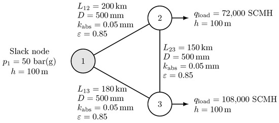
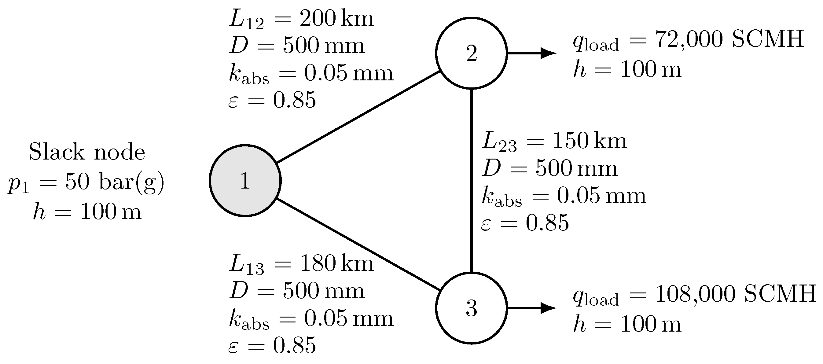
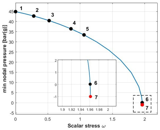
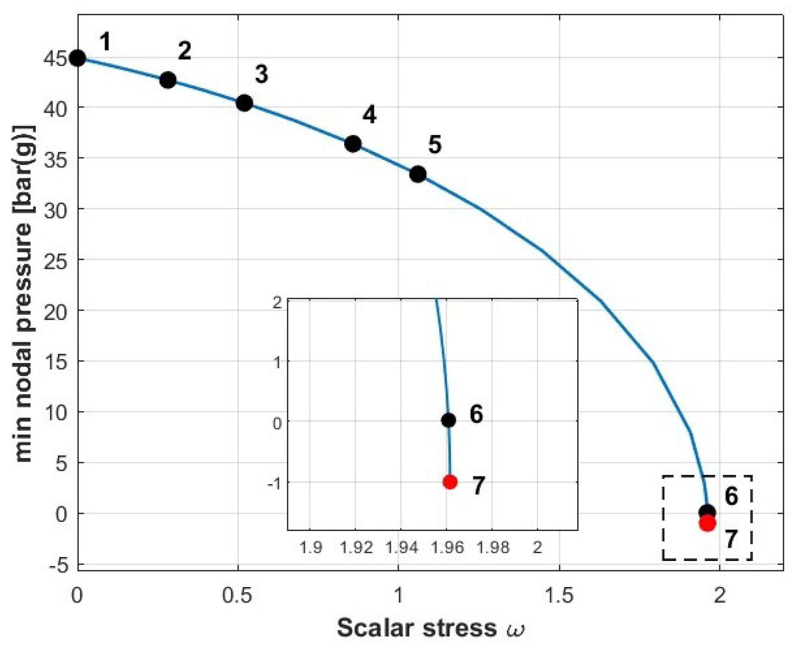
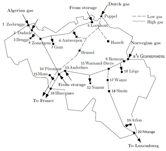
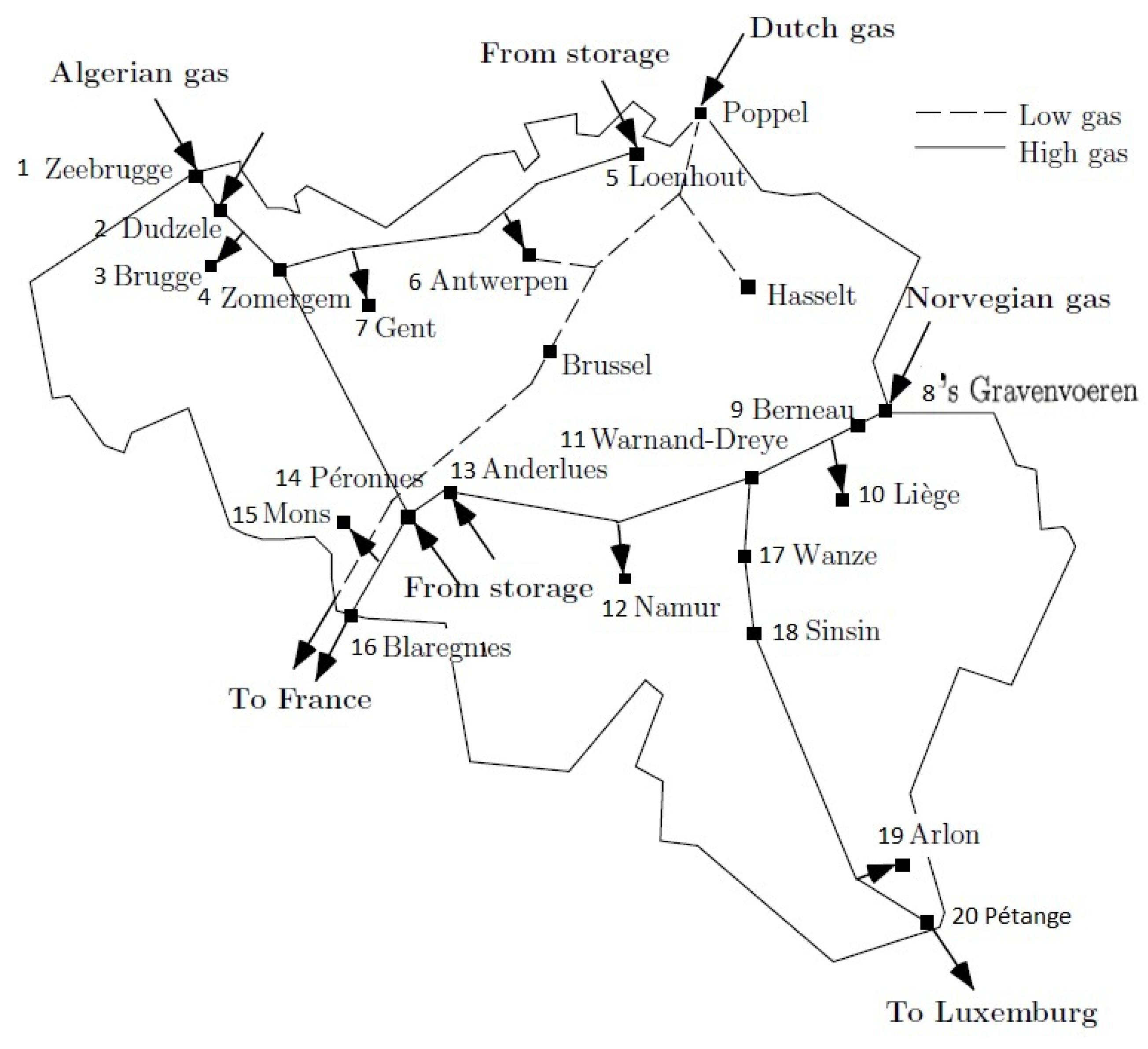
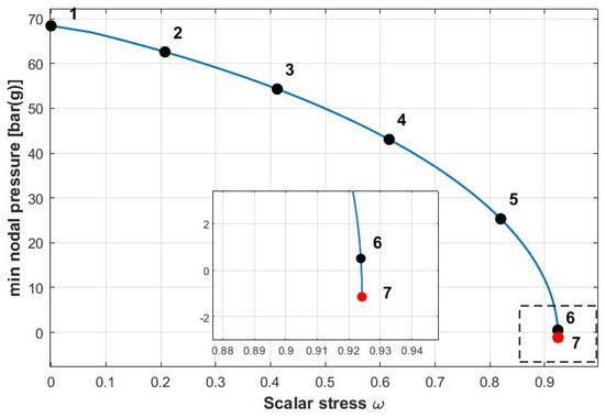
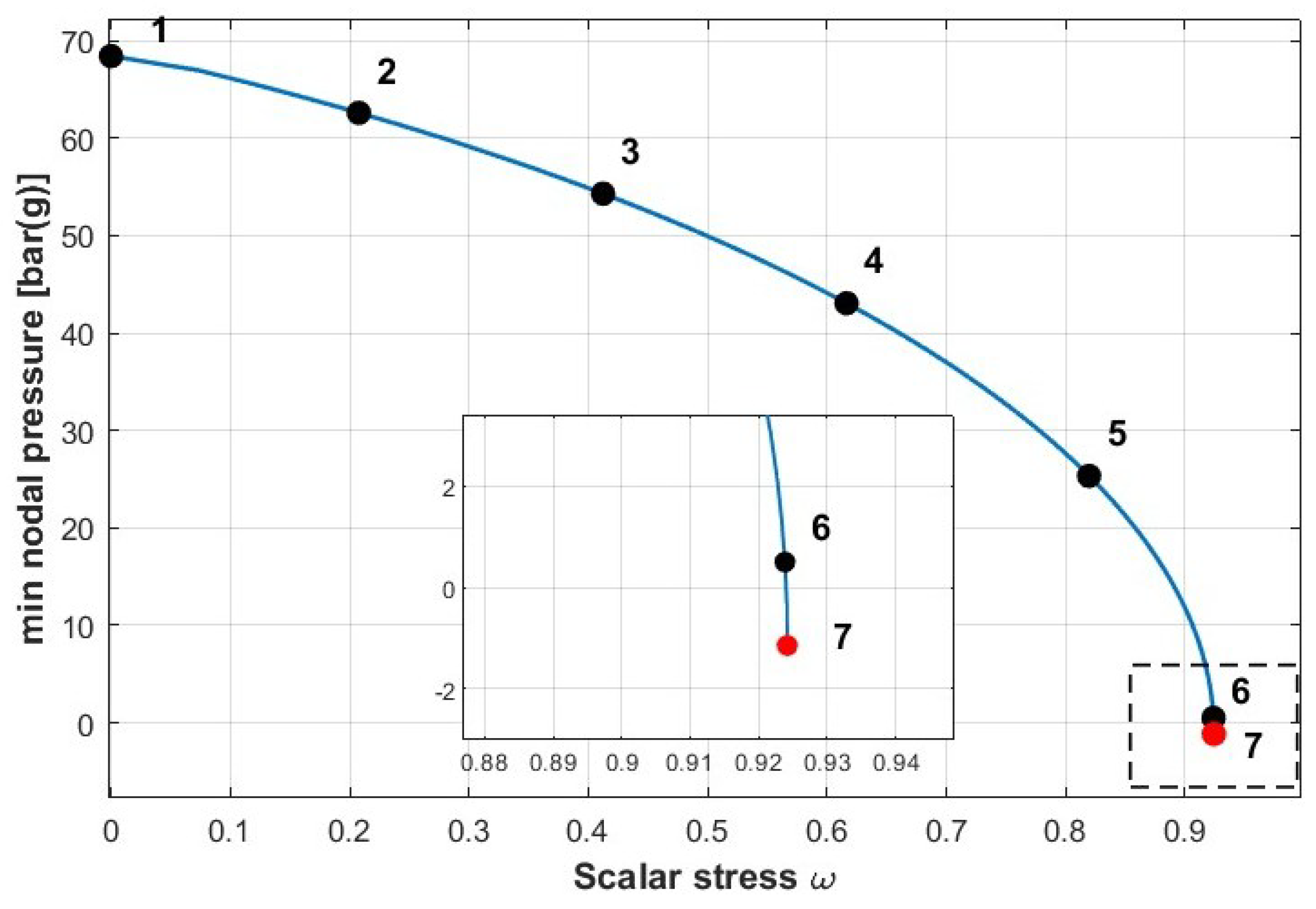
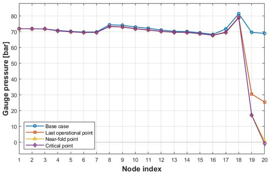
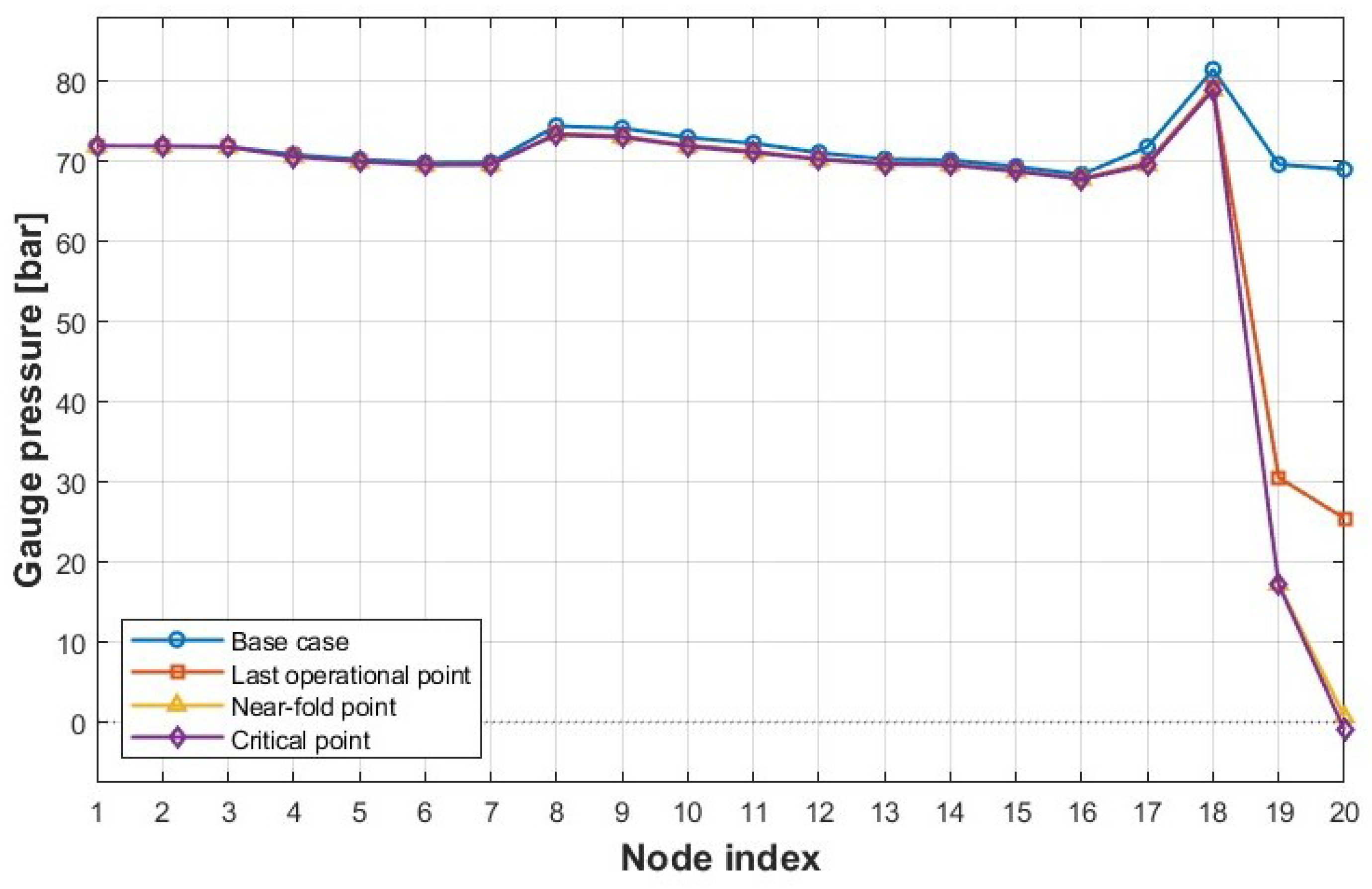
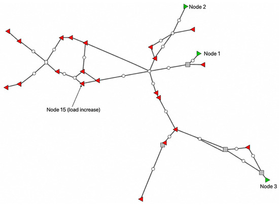
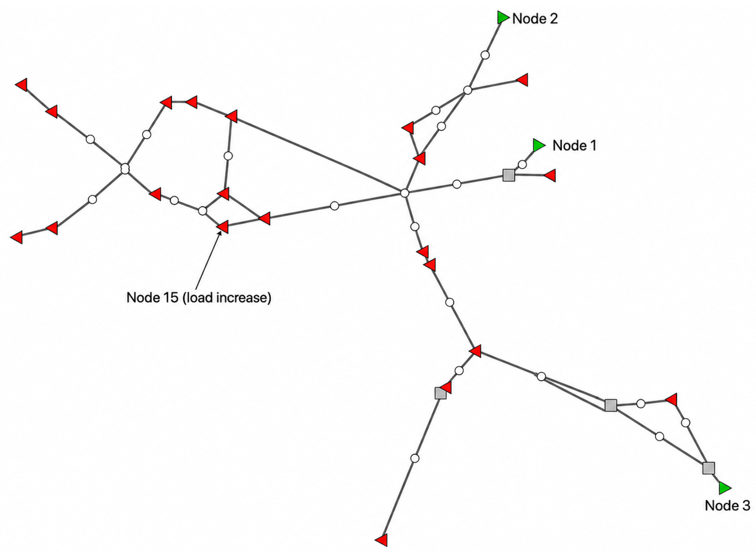
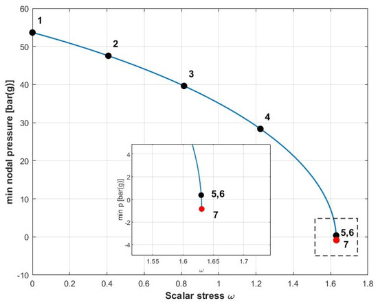
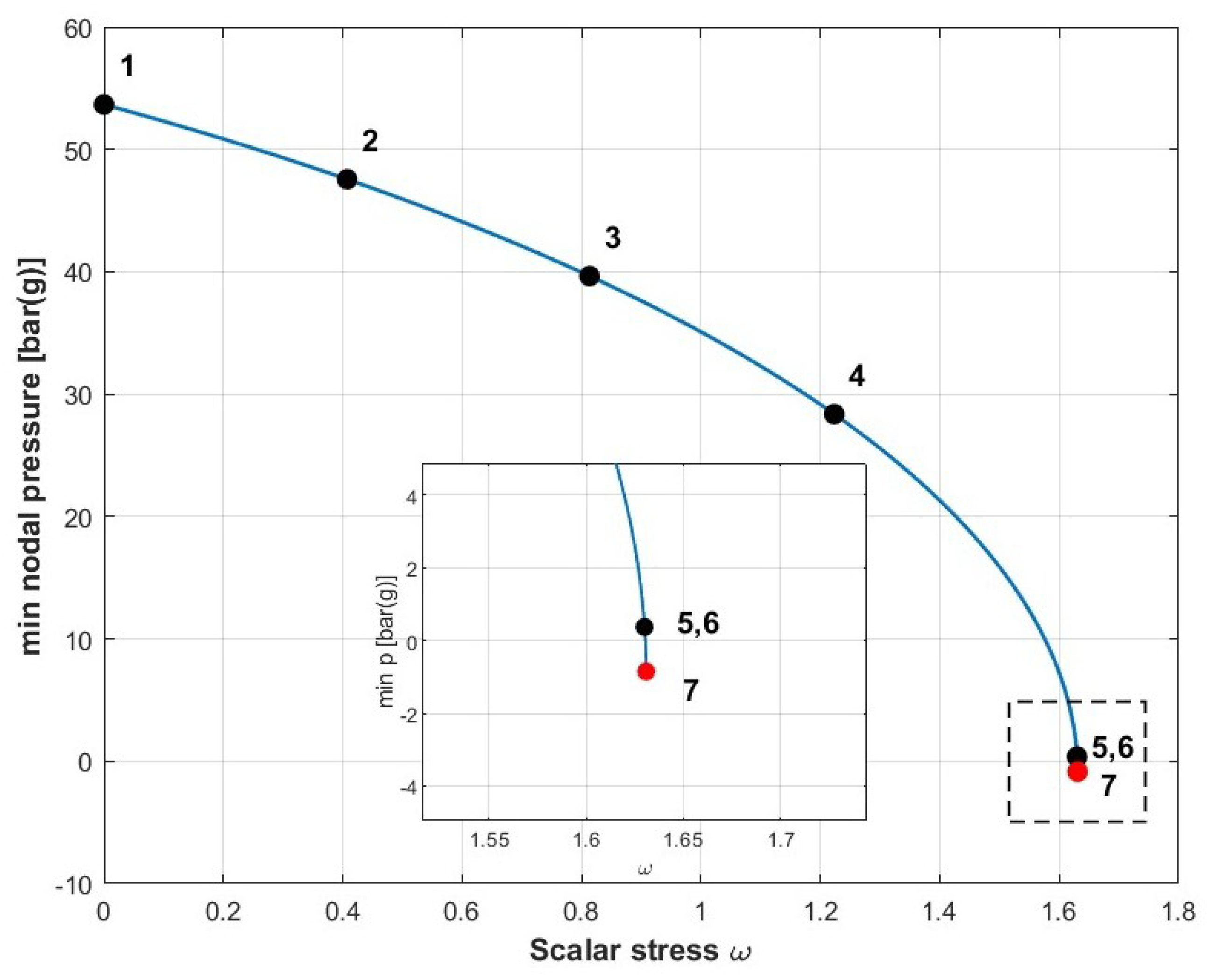
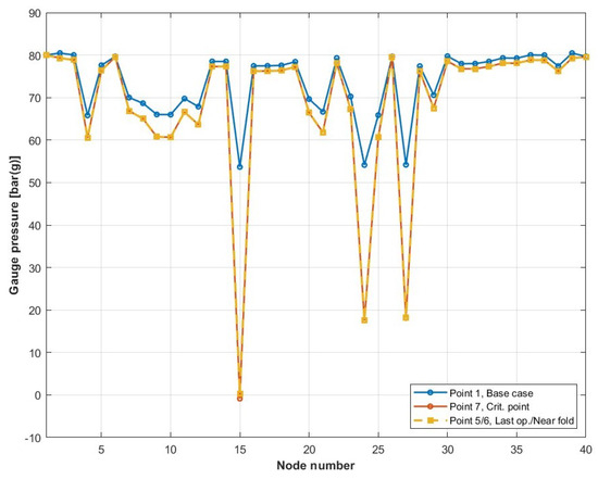
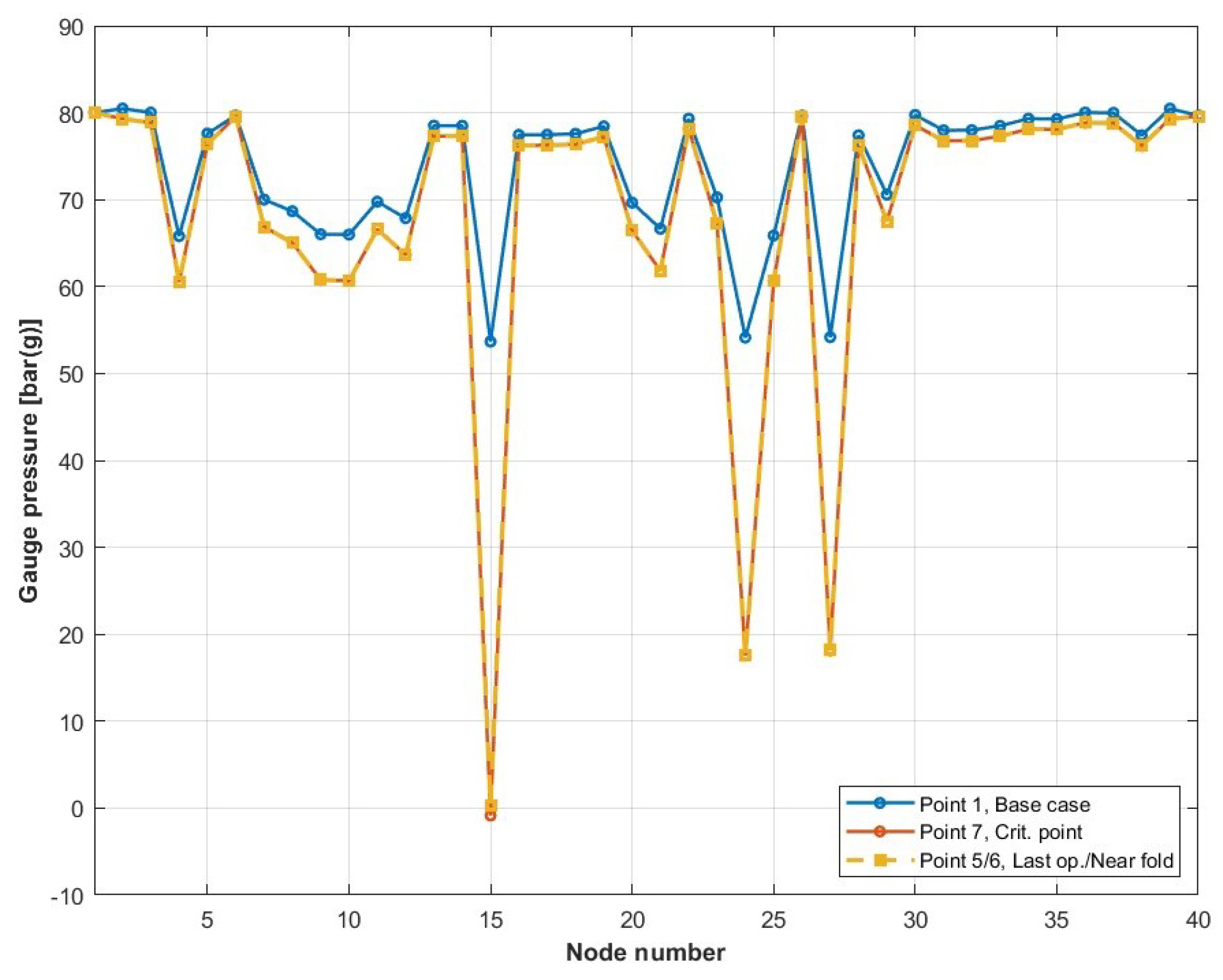

Disclaimer/Publisher’s Note: The statements, opinions and data contained in all publications are solely those of the individual author(s) and contributor(s) and not of MDPI and/or the editor(s). MDPI and/or the editor(s) disclaim responsibility for any injury to people or property resulting from any ideas, methods, instructions or products referred to in the content. |
© 2026 by the authors. Licensee MDPI, Basel, Switzerland. This article is an open access article distributed under the terms and conditions of the Creative Commons Attribution (CC BY) license.