


Abstract
Mountain photovoltaic (PV) stations are increasingly deployed in complex terrain, where generation is jointly controlled by solar-resource variability, near-surface meteorology, and local topography. However, the quantitative contribution of topographic factors to regional-scale PV generation remains insufficiently evaluated, and many prediction studies rely on single-station or short-term records. In this study, monthly measured generation from 118 standardized village-level mountain PV stations in Badong County, western Hubei Province, China (2019–2021), was integrated with Solargis Global Horizontal Irradiance (GHI)-related solar-resource data, high-resolution gridded meteorological data, a 25 m digital elevation model, seasonal-cycle variables, and historical-generation features. After seasonally grouped median-absolute-deviation (MAD) outlier screening, GIS-based spatial matching, terrain extraction, and viewshed-derived shading analysis, regression models and climatology baselines were compared under both chronological validation and station-exclusion spatial cross-validation. Under the strict chronological validation, CatBoost achieved the best temporal performance among the tested models (R2 = 0.3119, MAE = 2719.7 kWh, RMSE = 3245.6 kWh), slightly outperforming the monthly climatology baseline. In the station-exclusion spatial cross-validation, XGBoost achieved the highest mean R2 (0.8659), indicating good spatial transferability to unseen stations. Correlation and partial-correlation analyses showed that the temperature-related variable group and monthly radiation were the dominant meteorological controls, whereas elevation, slope, and terrain shading showed weak direct correlations with monthly generation for already-sited stations. Annual 90% prediction intervals were further estimated using residual bootstrapping, with an empirical coverage of 94.9%. The proposed framework provides a practical basis for monthly generation forecasting and operational assessment of already-built distributed PV stations in mountainous regions, while its application to greenfield site selection requires additional site engineering and near-field obstruction information.
1. Introduction
The rapid expansion of photovoltaic (PV) power generation is a central pathway for reducing fossil-fuel dependence and supporting low-carbon energy transitions. Compared with conventional generation resources, PV systems are strongly affected by the temporal variability of solar radiation, cloud conditions, temperature, and local operating conditions [1,2]. This variability poses challenges for power-system balancing, electricity trading, and storage scheduling [3]. Accurate PV generation prediction is therefore essential for high-penetration renewable energy integration and the reliable operation of distributed PV assets.
PV generation is controlled by coupled physical, meteorological, and engineering factors. Solar irradiance is the direct energy source, while seasonal solar geometry, cloudiness, precipitation, relative humidity, and aerosol conditions influence the effective radiation received by PV modules. Temperature affects module conversion efficiency through thermal derating, and equipment characteristics such as inverter efficiency, DC/AC sizing, curtailment, and maintenance status can further modify generation. In mountainous regions, terrain introduces additional spatial heterogeneity through elevation, slope, aspect, terrain obstruction, and local microclimate gradients.
Previous PV prediction studies have developed physical models, statistical time-series models, machine-learning algorithms, and deep-learning architectures, as systematized in recent comprehensive reviews [4,5]. Physical models link numerical weather prediction and PV system parameters through radiation-transfer and module-performance equations, whereas statistical models are computationally efficient but are often limited under nonlinear and nonstationary weather conditions. Machine-learning approaches such as ensemble methods have been shown to capture nonlinear relationships between meteorological variables and PV output [6,7], and long-term studies further indicate that PV generation is sensitive to climate variability [8]. Among ensemble algorithms, random forests [9] and gradient-boosted trees, including LightGBM [10] and XGBoost [11], are widely used because they capture nonlinear feature interactions, handle mixed-scale predictors, and require limited feature engineering. CatBoost extends the framework with ordered boosting to reduce target leakage [12], and the contribution of each predictor can be interpreted with built-in importance scores or SHAP-based attribution [13]. More recently, attention-based architectures [14] and deep neural network models for solar power forecasting [15] have been developed, and spatio-temporal graph models have been introduced to capture temporal and spatial dependencies among multiple PV stations [16].
Despite these advances, three gaps remain important for mountain PV applications. First, most studies emphasize meteorological factors such as irradiance and temperature, whereas terrain factors such as elevation, slope, aspect, and surrounding landform obstruction are less frequently quantified within a unified prediction framework, even though terrain has been shown to strongly modulate solar resource availability and local microclimate in mountainous regions [17,18]. Second, many studies are based on a single PV plant or short-term power data, which limits their ability to assess model generalization across heterogeneous terrain [19,20]. Third, regional-scale PV assessment requires the integration of measured generation, gridded meteorology, solar-resource products, and DEM-derived terrain attributes [21,22], but practical workflows for such multi-source fusion remain underdeveloped.
To address these gaps, this study uses 118 standardized mountain PV stations in a representative mountainous county of western Hubei Province, China, as a regional sample. The objectives are to (1) characterize the spatial and seasonal variability of monthly PV generation in a mountainous county, (2) construct a multi-source prediction framework that jointly incorporates meteorological, topographic, seasonal, and historical-generation predictors, (3) compare regression models and climatology baselines under strict chronological validation, (4) evaluate spatial transferability using station-exclusion spatial cross-validation, and (5) quantify the relative roles of radiation, temperature-related variables, precipitation, humidity, terrain attributes, and historical generation while explicitly considering feature collinearity and prediction uncertainty.
The novelty of this study does not lie in proposing a new machine-learning algorithm, because XGBoost, LightGBM, and CatBoost have already been widely used in PV forecasting. Rather, the contribution is the construction and evaluation of a regional multi-source framework for standardized mountain PV stations. The framework jointly incorporates measured generation, GHI-related solar-resource information, gridded meteorological variables, DEM-derived terrain attributes, viewshed-based terrain obstruction, historical generation features, climatology baselines, chronological validation, and station-exclusion spatial cross-validation. This design allows us to distinguish temporal generalization from spatial transferability and to evaluate whether terrain indicators still provide direct predictive information after engineering site selection has already taken place.
2. Materials and Methods
2.1. Study Area
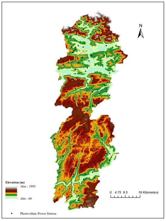
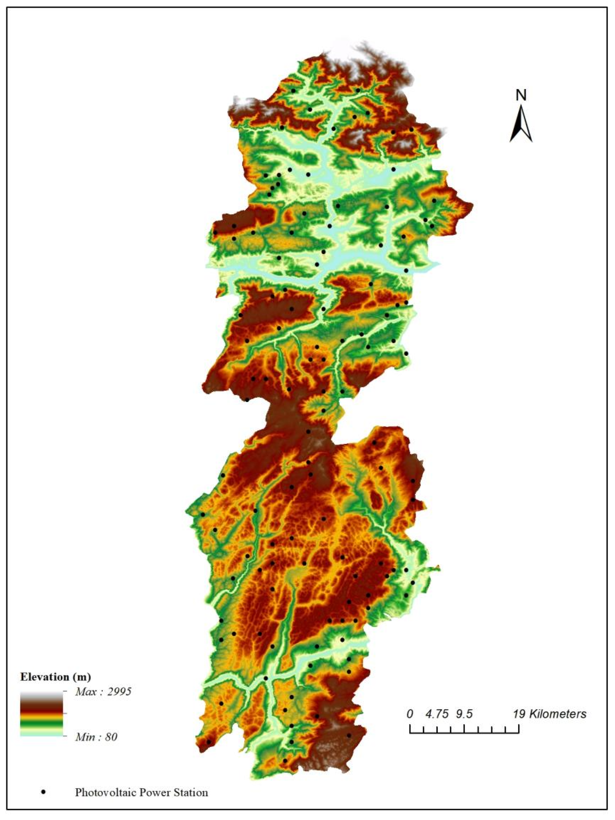
The study area is located in western Hubei Province, China, within the Wuling mountainous region and the Three Gorges area of the Yangtze River. The county has a long north–south extent and a narrow east–west width, with strong relief and complex terrain. Mountains account for most of the area, while plains and river terraces are mainly distributed along the Yangtze River, Qingjiang River, and small intermountain basins. Such topographic complexity creates substantial spatial variation in solar radiation, temperature, terrain shading, and station accessibility, making the county a representative region for studying mountain PV generation. The spatial distribution of the 118 stations overlaid on DEM-derived elevation is shown in Figure 1.
Figure 1.
Distribution of the 118 village-level PV stations overlaid on DEM-derived elevation in the study area.
2.2. Data Sources
Monthly PV generation data were collected from 118 village-level PV stations in the study area from January 2019 to December 2021. All stations were constructed in 2018 and began operation in 2019. The stations have a unified installed capacity of 200 kW and were designed using 265 Wp polycrystalline PV modules with similar inverters and combiner-box configurations. This standardized design reduces the influence of installed capacity and equipment differences, allowing the analysis to focus on meteorological and topographic controls [19,20].
Solar-resource information was obtained from the Solargis global solar-energy dataset. The 1991–2020 mean annual total irradiation product and monthly Global Horizontal Irradiance (GHI)-related radiation variables were used to characterize the background solar-resource conditions and monthly radiation variability at each station. The annual total irradiation product has a spatial resolution of approximately 1 km × 1 km, while the monthly radiation variables were spatially matched to station locations together with gridded meteorological variables.
High-resolution gridded meteorological data were obtained from the China Meteorological Administration Land Data Assimilation System (CLDAS-V2.0), which has been shown to provide superior representation of near-surface temperature and humidity over China compared with global reanalysis products [22]. The variables included air temperature, maximum temperature, minimum temperature, precipitation, relative humidity, and radiation-related fields. The original hourly data with a spatial resolution of 0.01° × 0.01° were aggregated to the monthly scale and spatially matched to each PV station.
Topographic variables were derived from the ASTER Global Digital Elevation Model version 3 (GDEM V003) [21] with a spatial resolution of 25 m. Elevation, slope, and aspect were extracted for each PV station using GIS-based spatial analysis. A viewshed-based shading variable was further calculated to describe terrain obstruction around each station.
2.3. Data Cleaning and Spatial Matching
Because monthly distributed PV generation records may contain missing values, communication errors, and abnormal values caused by equipment faults, temporary maintenance, curtailment, or data-transmission problems, a seasonally grouped median absolute deviation (MAD) method was used for quality control. Instead of applying a single threshold to the full annual series, the MAD screening was performed separately for each calendar month across all stations and years, so that normal seasonal differences between winter and summer generation would not be misclassified as outliers.
For calendar month m, the monthly median and MAD were calculated as follows:
A monthly generation record was flagged as an outlier when:
where is the monthly generation record belonging to calendar month m, is the monthly median, and is the MAD multiplier. In this study, = 3 was used as the primary threshold. Among the original 4248 station-month records, 6 missing or non-positive records were removed, and 322 additional records were flagged by the seasonally grouped MAD screening. The final modeling dataset contained 3920 valid station-month samples. Sensitivity tests using = 4 and = 5 were further conducted to examine the influence of the MAD threshold. Relaxing the threshold retained more abnormal monthly records but reduced both chronological validation and station-exclusion spatial validation performance. Therefore, = 3 was retained as the primary quality-control threshold to ensure the reliability of the modeling samples.
After quality control, PV station points, gridded meteorological data, Solargis GHI-related radiation data, and DEM-derived terrain variables were spatially aligned in ArcGIS 10.8 (Esri, Redlands, CA, USA). Raster values were extracted at each station location after projection consistency checking and resampling where necessary.
2.4. Topographic Variables and Terrain Shading
Elevation, slope, and aspect were extracted directly from the preprocessed 25 m DEM. Terrain shading was quantified using a viewshed approach implemented with the ArcGIS 3D Analyst extension. Each PV station was treated as an observer point with a height of 2 m, corresponding approximately to the PV module height. A full 360° azimuth range around each station was considered, and all DEM cells within a 2000 m radius were used as the viewshed window. Therefore, the effective horizontal sampling resolution of the terrain-obstruction analysis was 25 m, consistent with the DEM resolution.
The output viewshed raster identified visible and obstructed cells around each station. A station-level shading ratio (SR) was calculated as follows:
where SR is the shading ratio (%), and and denote the numbers of obstructed and visible DEM cells within the viewshed window, respectively. A larger SR indicates stronger surrounding-terrain obstruction and a higher potential for terrain-related radiation loss. The calculated shading ratio represents only topographic obstruction by surrounding terrain. It does not include near-field obstructions such as trees, buildings, utility poles, local infrastructure, PV row-to-row shading, or temporary shading caused by vegetation growth. Therefore, the shading ratio should be interpreted as a regional terrain-obstruction indicator rather than a detailed module-level shading simulation.
2.5. Prediction Models and Feature Construction
Five regression models were compared: Ridge Regression, Random Forest (RF), LightGBM, XGBoost, and CatBoost. Ridge Regression was used as a regularized linear baseline, RF was used as a classical bagging-ensemble model, and LightGBM, XGBoost, and CatBoost were used as gradient-boosted tree models. In addition to these regression models, three climatology baselines were introduced: monthly climatology, station climatology, and station-month climatology. The monthly climatology uses the mean generation of the same calendar month in the training period; the station climatology uses the mean generation of the same station in the training period; and the station-month climatology uses the mean generation of the same station and calendar month in the training period. These baselines provide simple but practically meaningful references for evaluating whether machine-learning models add predictive skill beyond historical averages.
The original predictors included precipitation, average temperature, relative humidity, minimum temperature, maximum temperature, monthly radiation, elevation, slope, aspect, and shading ratio. To represent seasonal periodicity, two cyclic month variables were added:
where m is the calendar month. Historical-generation features were also constructed from the training period, including same-station monthly climatology, station mean generation, monthly mean generation, and a same-station monthly anomaly ratio. For the independent 2021 validation set, these historical features were calculated only from 2019 to 2020 records to avoid information leakage. Within the training period, leave-one-out historical features were used where necessary so that the target record itself was not used to construct its own predictor.
2.6. Validation Design and Evaluation Metrics
Two complementary validation strategies were used. First, a strict chronological validation was applied to evaluate temporal generalization: data from 2019 to 2020 were used for training, and data from 2021 were held out as an independent validation set. Second, station-exclusion spatial cross-validation was conducted to evaluate spatial transferability. In this experiment, entire stations were excluded from training and used only for testing, ensuring that no monthly records from the same test station were available during model fitting. This design provides a stricter test of whether the model can be transferred to unseen stations.
Model performance was evaluated using mean absolute error (MAE), root-mean-square error (RMSE), coefficient of determination (R2), and mean bias error, defined as observed minus predicted generation. The metrics are defined as follows:
where and are the observed and predicted monthly generation values for sample i, ȳ is the mean observed generation, and n is the number of validation samples.
2.7. Hyperparameter Settings and Statistical Tests
The final model settings were selected by minimizing temporal-validation RMSE, with MAE and R2 used as supplementary metrics. The final hyperparameters used in the revised analysis are summarized in Table 1. For each model, the hyperparameters were tuned by grid search over the ranges listed below, and the final settings were selected by minimizing the 2021 temporal-validation RMSE, with MAE and R2 as supplementary metrics. The search ranges were as follows. Ridge Regression: alpha ∈ {0.1, 1.0, 5.0, 10.0}. Random Forest: n_estimators ∈ {100, 200, 300}, max_depth ∈ {4, 5, 6, 8, None}, min_samples_leaf ∈ {3, 5, 8, 10}. LightGBM: n_estimators ∈ {80, 120, 160, 200}, learning_rate ∈ {0.03, 0.05, 0.08}, max_depth ∈ {2, 3, 4}, num_leaves ∈ {5, 7, 15}, min_child_samples ∈ {20, 30, 50}, reg_lambda ∈ {1.0, 5.0, 10.0}. XGBoost: the same n_estimators, learning_rate and max_depth ranges, with min_child_weight ∈ {3, 5, 8, 10}, reg_lambda ∈ {1.0, 5.0, 10.0} and reg_alpha ∈ {0.0, 0.1, 0.5}. CatBoost: iterations ∈ {80, 120, 160, 200}, learning_rate ∈ {0.03, 0.05, 0.08}, depth ∈ {2, 3, 4}, l2_leaf_reg ∈ {3.0, 10.0, 20.0}. All regression models were implemented in Python using the scikit-learn, XGBoost, LightGBM, and CatBoost libraries.
Table 1.
Search ranges considered and final hyperparameter settings of the compared regression models.
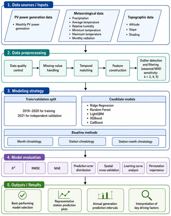
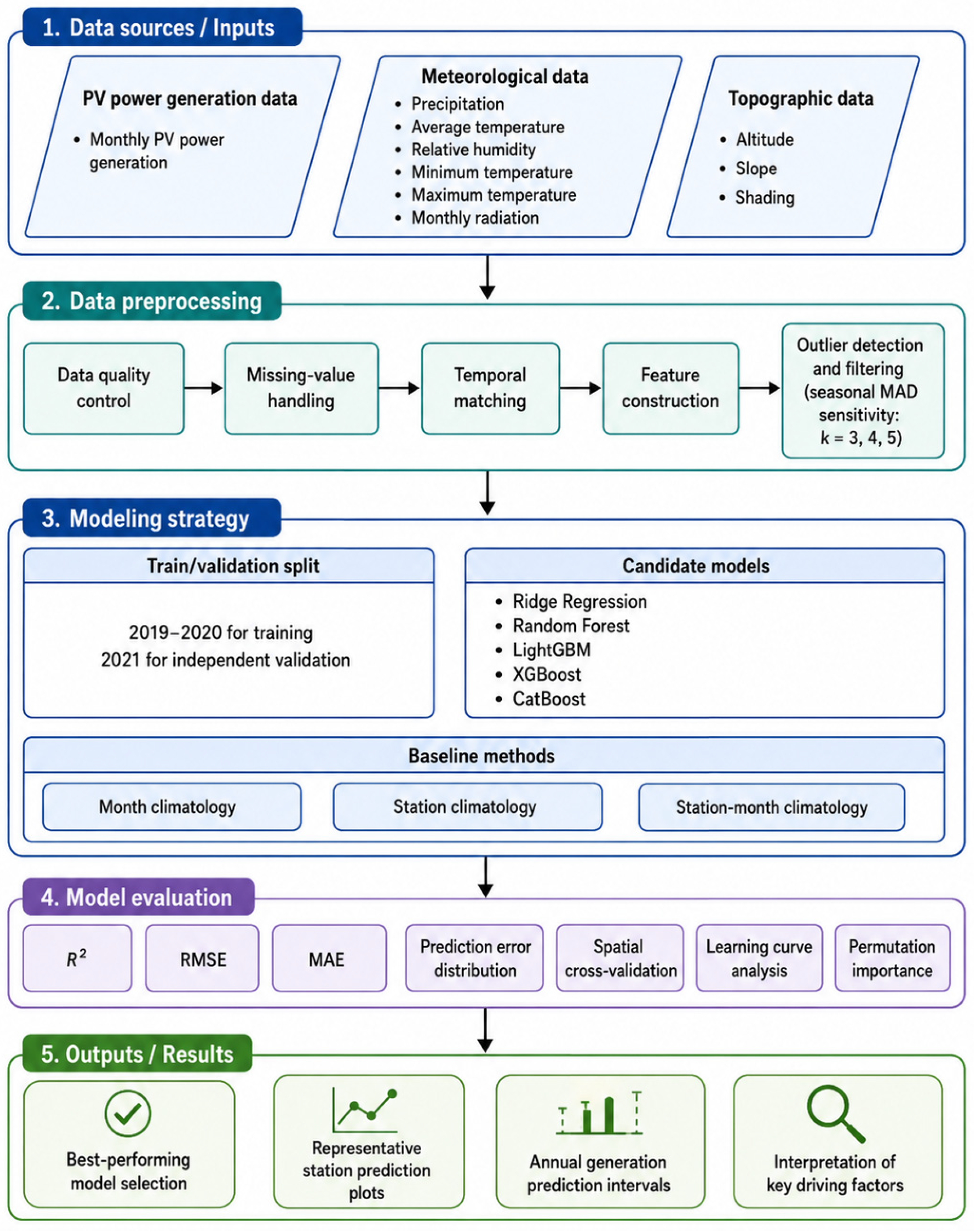
Paired Wilcoxon signed-rank tests were applied to the absolute prediction errors from the same 2021 validation samples to compare model accuracy, with CatBoost—the best temporal-validation model—used as the reference model for all pairwise comparisons against the other models and the climatology baselines. Because seven comparisons were made against the reference model, the resulting one-sided p-values were adjusted using the Holm–Bonferroni correction. The overall workflow of the proposed multi-source meteorological–topographic modeling framework is shown in Figure 2.
Figure 2.
Workflow of the multi-source meteorological–topographic modeling framework for monthly PV power generation prediction.
3. Results
3.1. Background Solar Resource and Station Generation Differences
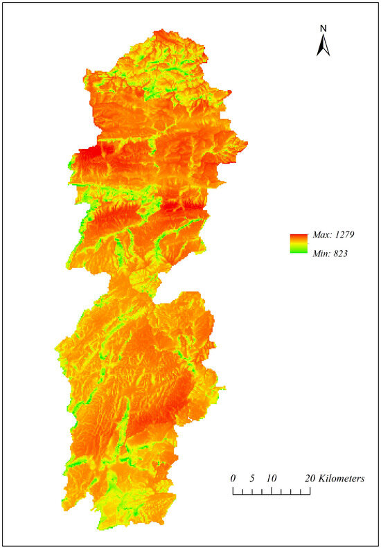
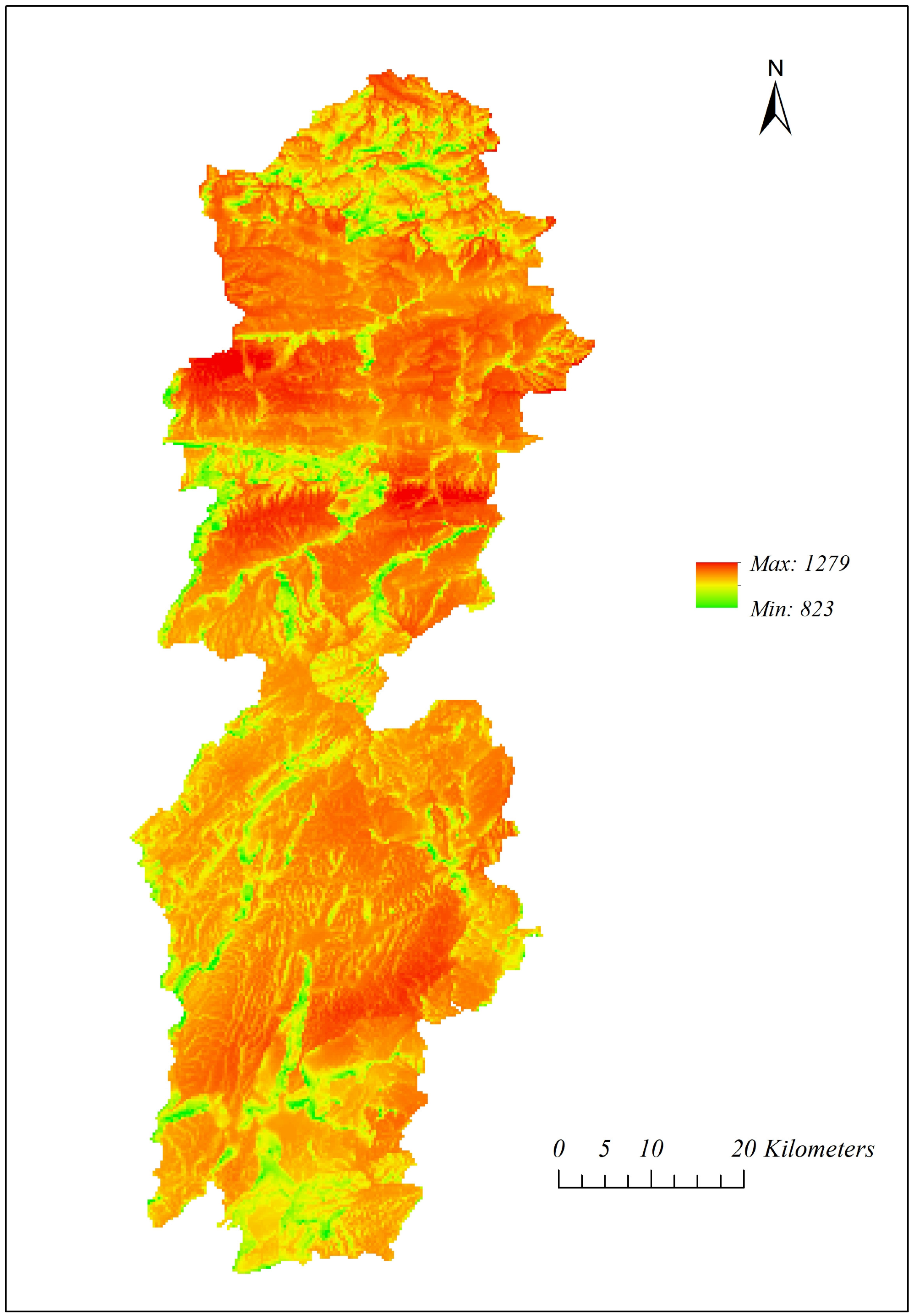
The annual total solar irradiation in the study area ranges from approximately 823 to 1279 kWh m−2 (Figure 3), indicating strong spatial heterogeneity. Higher-irradiation areas are mainly located in the central-northern and southern open terrain, where annual total irradiation locally exceeds 1200 kWh m−2. Lower-irradiation areas are mainly found in deeply incised valleys, steep slopes, and terrain-shaded areas, where irradiation can be below 900 kWh m−2. This distribution suggests that mountain landforms strongly modulate the background solar-resource potential.
Figure 3.
Spatial distribution of annual total solar irradiation in the study area based on Solargis data.
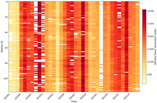
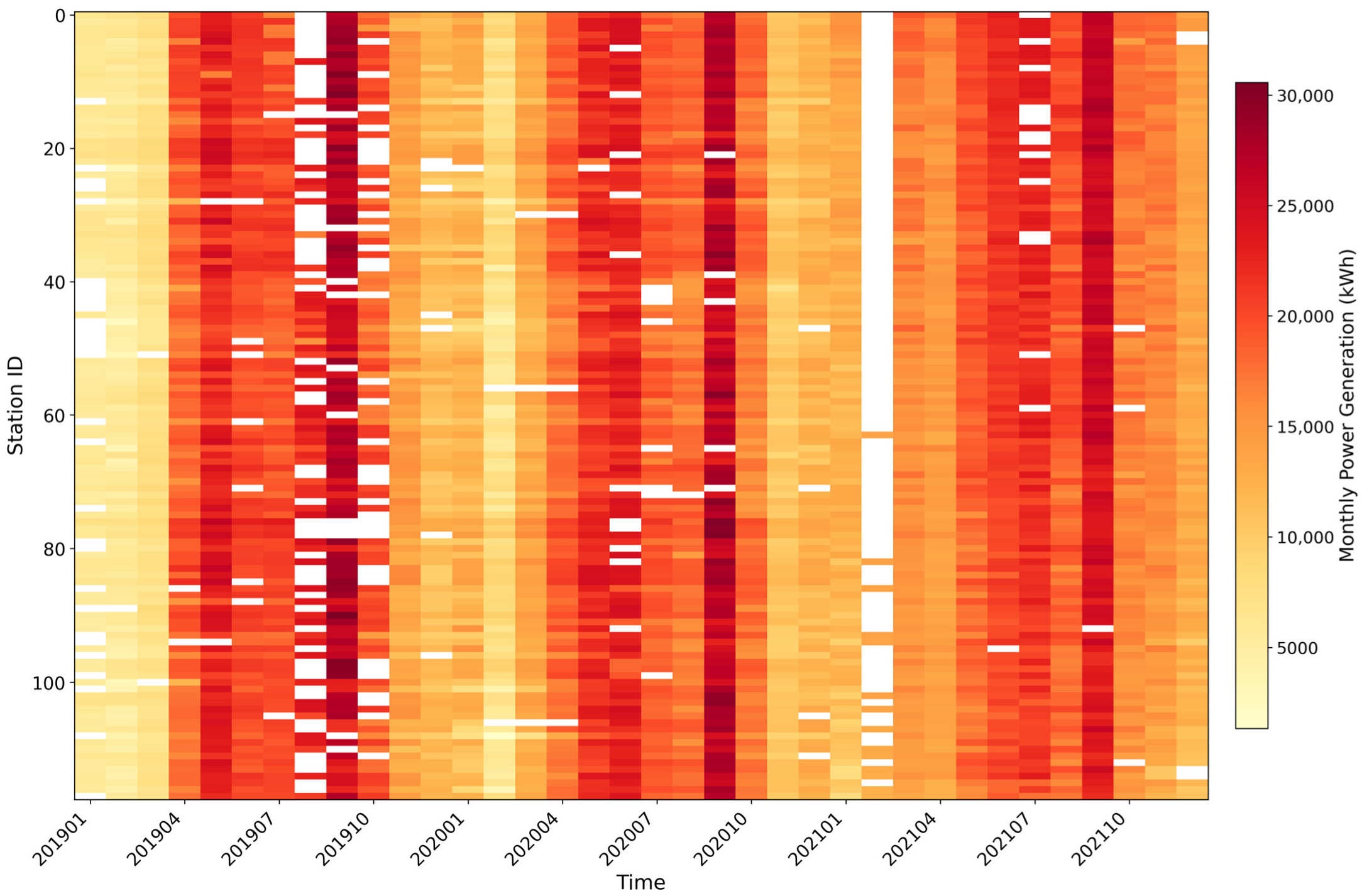
The monthly generation heatmap (Figure 4) shows clear seasonal variation across the 118 PV stations. High generation is concentrated from April to September, while low generation mainly occurs from November to February of the following year. This pattern is consistent with seasonal changes in solar elevation angle, day length, and regional meteorological conditions. The heatmap also reveals station-to-station differences under the same monthly climate background, highlighting the combined effects of local radiation resources, terrain, and station-specific operation. White cells in Figure 4 represent missing records or samples removed by the quality-control procedure rather than zero generation.
Figure 4.
Spatiotemporal distribution of monthly PV generation for the 118 stations during 2019–2021. Rows represent station IDs and columns represent months. White cells indicate missing records or samples removed during quality control.
Based on the three-year mean annual utilization hours, calculated following the photovoltaic performance-monitoring conventions of IEC 61724-1 [23], classified as General or Moderate (Table 2), while only three stations reached the Good class and no station reached the Excellent class. The average annual utilization hours of the 118 stations was 916.7 h, ranging from 796.1 to 1013.2 h. This indicates that the village-level mountain PV stations in the study area generally had moderate-to-low utilization levels, with clear station-to-station differences. Because all stations had the same installed capacity of 200 kW, monthly generation and utilization hours contain equivalent information within this dataset; however, utilization hours provide a more transferable indicator for comparison with stations of other capacities.
Table 2.
Classification of PV-station generation capability based on annual utilization hours.
3.2. Model Performance Comparison
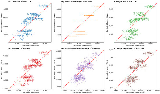
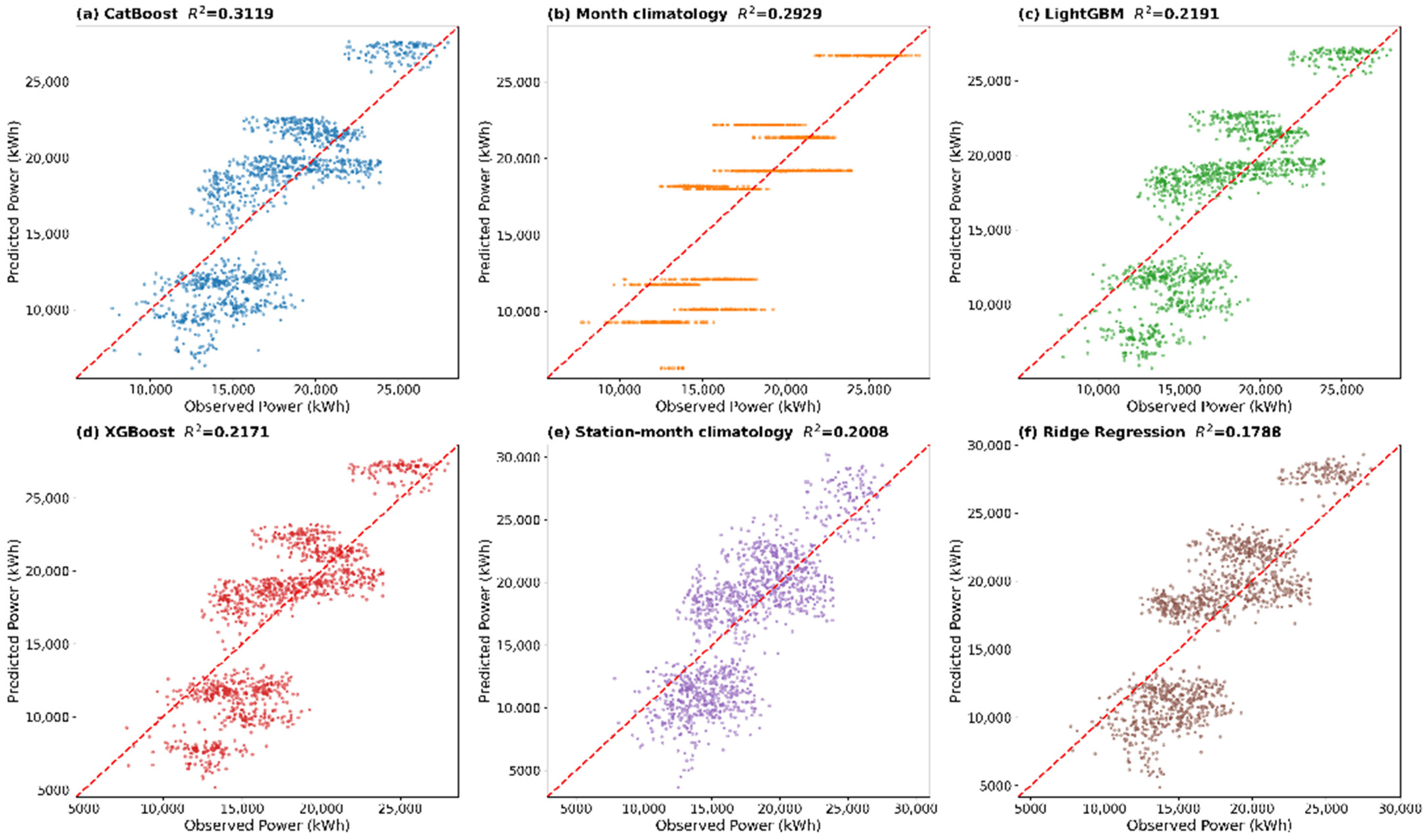
The observed-versus-predicted scatter plots in Figure 5 show that the tested models and climatology baselines captured the broad range of monthly PV generation, but their temporal-validation skills differed substantially. CatBoost produced the best numerical temporal-validation performance among the tested models (Table 3), although the scatter distribution still shows clear stratification and non-negligible deviations from the 1:1 line. This stratified pattern indicates that the models mainly captured seasonal generation levels and historical station characteristics rather than all interannual and operational variations in 2021. The monthly climatology baseline also performed competitively, suggesting that the seasonal cycle is a strong predictor of monthly PV generation.
Figure 5.
Observed versus predicted monthly PV generation in the independent 2021 validation period for the selected models and climatology baselines: (a) CatBoost; (b) Month climatology; (c) LightGBM; (d) XGBoost; (e) Station-month climatology; and (f) Ridge Regression. The red dashed line denotes the 1:1 line.
Table 3.
Chronological validation performance in the independent 2021 validation period. Error statistics are in kWh.
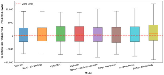
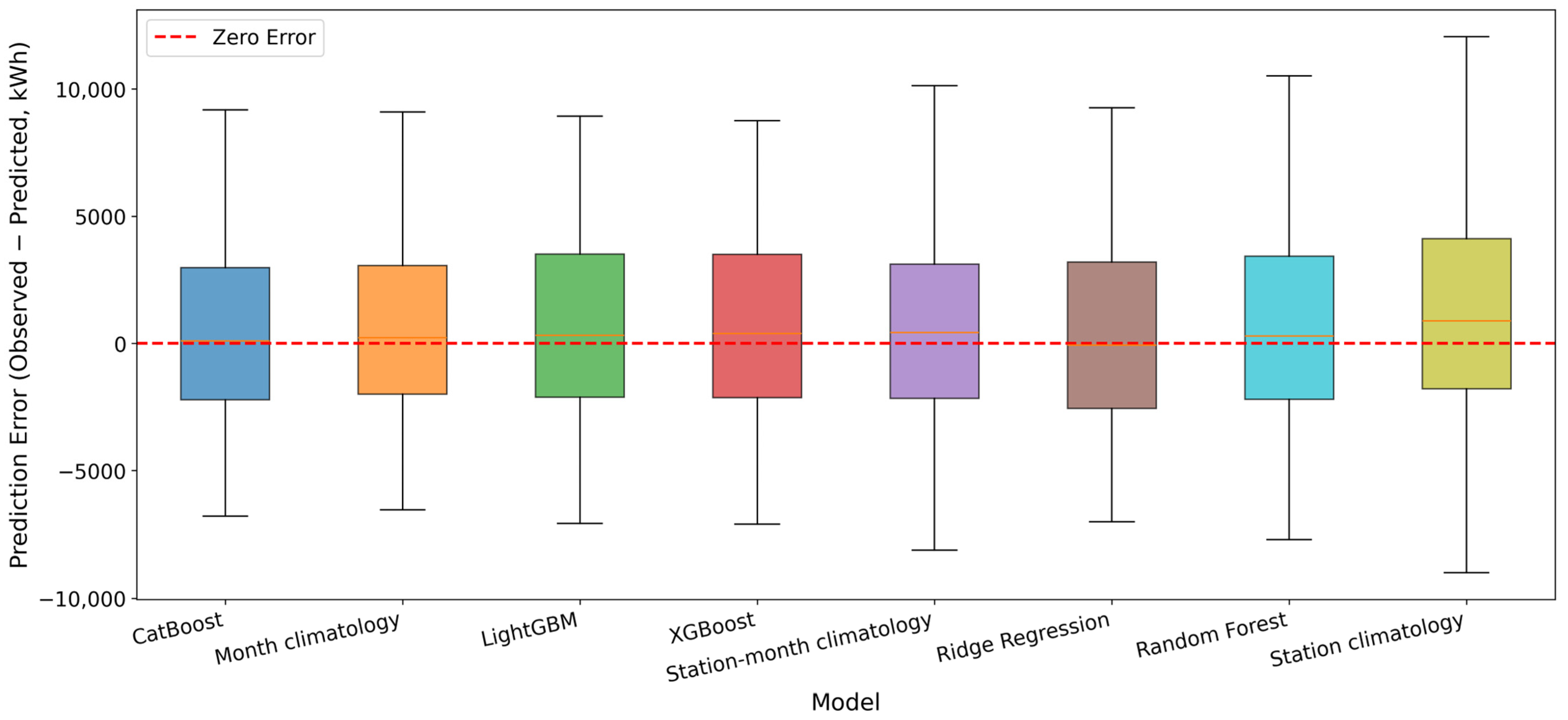
The prediction-error boxplots further compare the error distributions of the models and climatology baselines in the independent 2021 validation period (Figure 6). The median errors of most models are close to zero, but their interquartile ranges differ. CatBoost has the best overall temporal-validation performance and a relatively small mean bias. The month’s climatology baseline also shows a competitive error distribution, consistent with the strong seasonal control of monthly PV generation.
Figure 6.
Boxplot comparison of prediction errors, defined as observed minus predicted monthly generation, in the independent 2021 validation period.
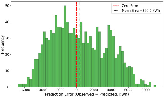
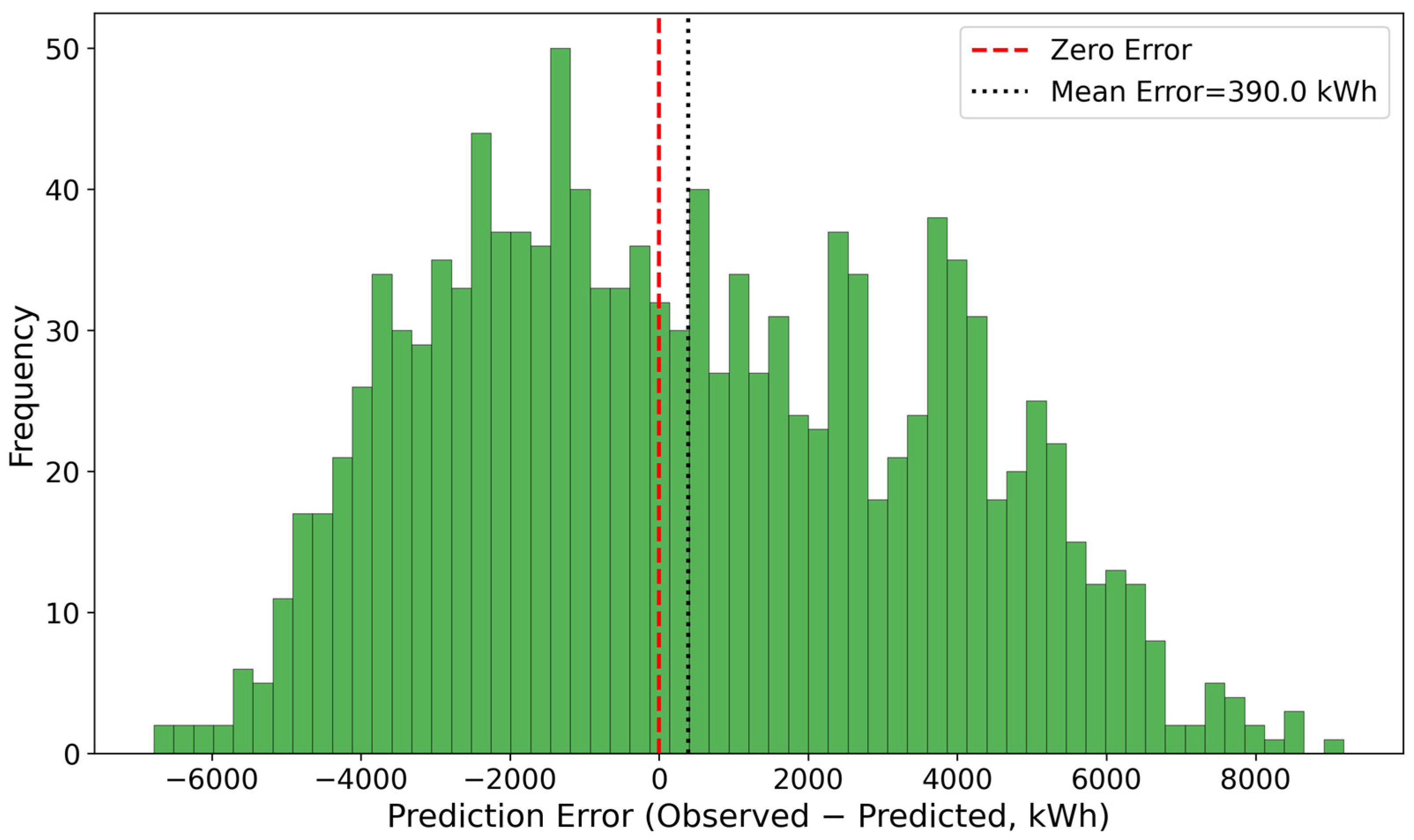
For CatBoost, the mean error, defined as observed minus predicted generation, is 390.0 kWh (Figure 7), indicating a slight underestimation of 2021 monthly generation. This systematic offset may be associated with interannual differences between the 2019–2020 training period and the 2021 validation period, as well as unobserved operational factors such as maintenance, cleaning, soiling, curtailment, and inverter status. The relatively broad and asymmetric error distribution also indicates that some station-month samples were still affected by unobserved operational or interannual factors.
Figure 7.
Error distribution of the CatBoost model in the independent 2021 validation period. The red dashed line denotes zero error, and the black dotted line denotes the mean error.
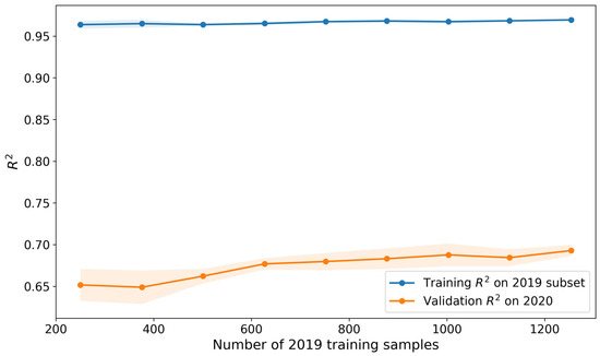
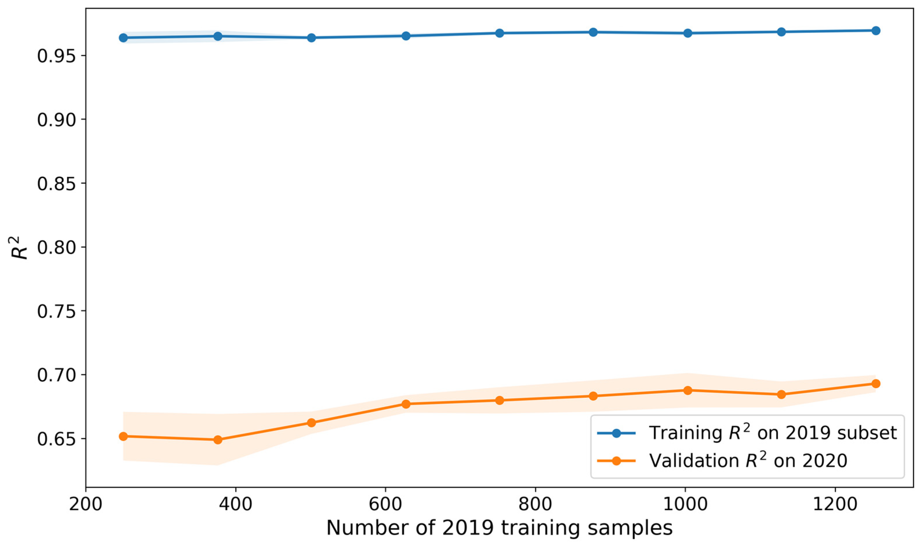
CatBoost, the best temporal-validation model, was also used for the learning-curve diagnosis (Figure 8). The learning curve was calculated without using the independent 2021 validation set: the model was trained using progressively enlarged subsets of the 2019 samples and evaluated on the 2020 samples. The training R2 remained around 0.96–0.97, while the validation R2 on 2020 increased from approximately 0.65 to 0.69 as the training sample grew, without a decline at the largest training size. The persistent gap of about 0.27 between the training and validation R2 indicates that the model fits the training period well but retains a non-negligible generalization gap under the limited two-year training record.
Figure 8.
CatBoost learning curve calculated without using the independent 2021 validation set.
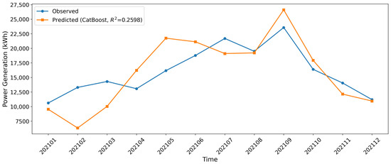
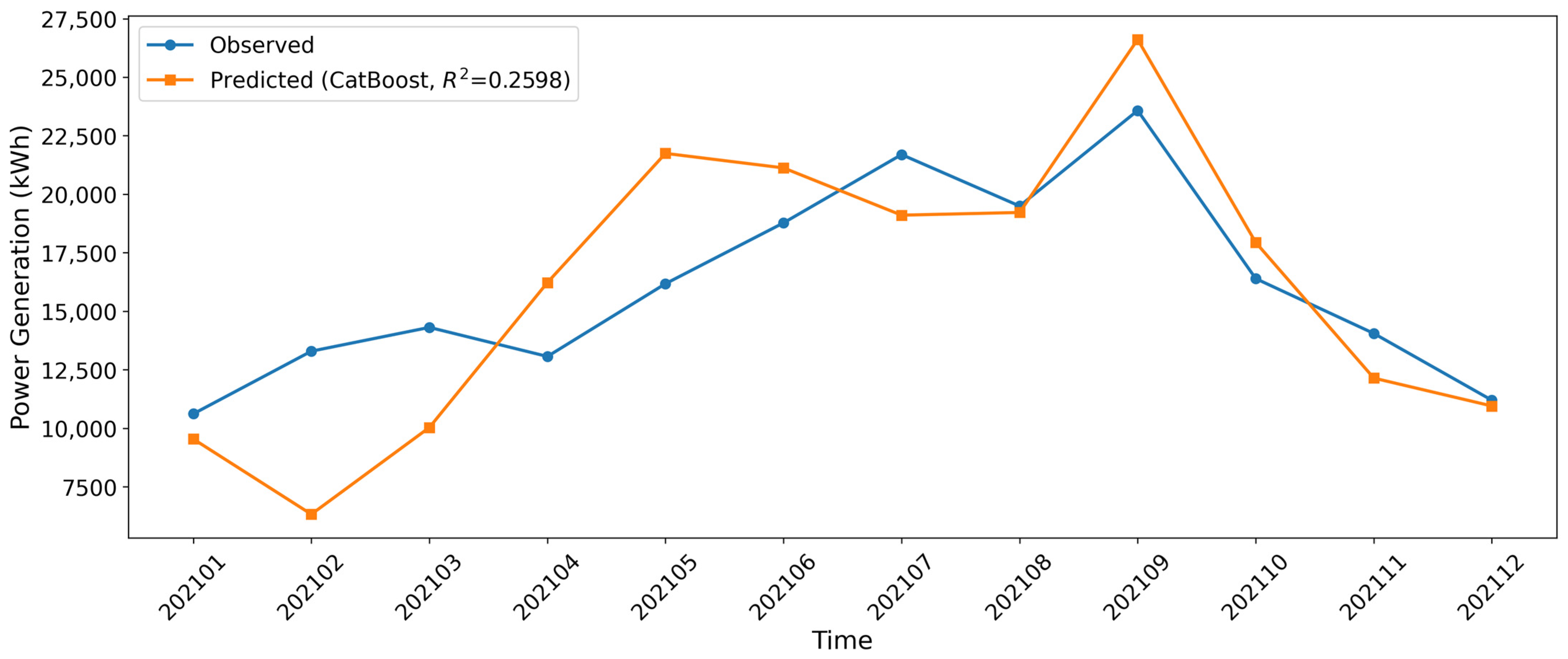
A representative station was selected to illustrate the ability of the model to reproduce the seasonal cycle at the station scale. Across the 118 stations, the station-level R2 of CatBoost in 2021 ranged from −0.53 to 0.76, with a median of 0.26, and 76% of the stations had a positive R2. To avoid showing only the best case, a station close to the median skill was selected as the example (Station 111, station-level R2 = 0.26). The model broadly captured the low-generation winter months and the high-generation summer peak (Figure 9), although month-to-month deviations remained at this typical-performance station. This example, together with the wide station-level R2 range, demonstrates that the model can reproduce the broad seasonal evolution but that station-level performance varies considerably and should not be interpreted as uniform across all stations.
Figure 9.
Monthly observed and predicted PV generation for a representative station with median (typical) validation performance in 2021 (Station 111) using the CatBoost model.
To test whether the differences in chronological-validation accuracy were statistically significant, paired Wilcoxon signed-rank tests were applied to the absolute prediction errors of the 2021 validation samples, using CatBoost as the reference model and the Holm–Bonferroni correction for the seven comparisons (Table 4). CatBoost produced significantly smaller absolute errors than LightGBM, XGBoost, Random Forest, Ridge Regression, the station climatology, and the station-month climatology (Holm-adjusted p < 0.05 in all cases). However, the difference between CatBoost and the monthly climatology baseline was small and not statistically significant (Holm-adjusted p = 0.299). This confirms that, under strict chronological validation, the machine-learning models provide only a marginal and statistically insignificant gain over the seasonal-cycle baseline, and we therefore avoid overstating the superiority of any single model.
Table 4.
Paired Wilcoxon signed-rank tests of absolute prediction errors in the independent 2021 validation period, with CatBoost (mean absolute error = 2719.7 kWh) as the reference model.
3.3. Station-Exclusion Spatial Cross-Validation
The station-exclusion spatial cross-validation produced substantially higher R2 values than the strict chronological validation. XGBoost achieved the highest mean R2 (0.8659) and the lowest mean RMSE (2075.8 kWh) (Table 5), followed closely by LightGBM and Random Forest. Random Forest showed the lowest mean MAE (1606.3 kWh), but its mean R2 was slightly lower than that of XGBoost and LightGBM. These results indicate that tree-based models have good spatial transferability to unseen stations under the same multi-year sample period. The contrast between the relatively high spatial-validation skill and the moderate 2021 temporal-validation skill suggests that spatial transfer is easier than cross-year extrapolation for the present three-year dataset.
Table 5.
Station-exclusion spatial cross-validation performance. Error statistics are in kWh.
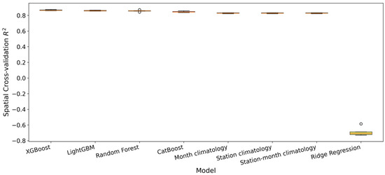
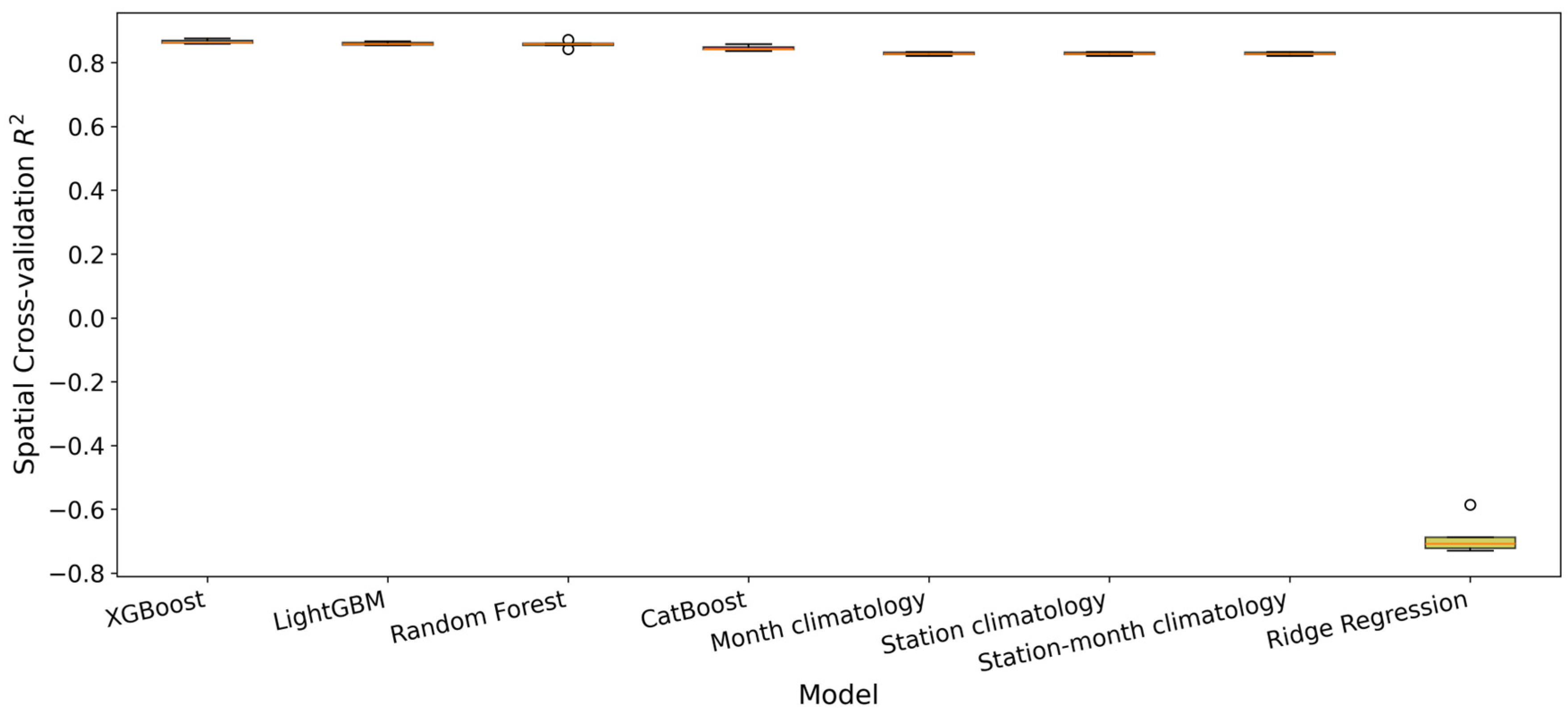
The distribution of fold-wise spatial cross-validation R2 values is further shown in Figure 10. The tree-based models consistently achieved high spatial-validation skill, with XGBoost, LightGBM, Random Forest, and CatBoost all showing R2 values above 0.84 on average. In contrast, Ridge Regression performed poorly in the station-exclusion experiment, indicating that linear relationships were insufficient to represent spatial transferability under complex mountain conditions. The high spatial-validation scores should be interpreted as transferability among already-built stations within the same regional sample period rather than as evidence of unrestricted generalization to new regions or future climate conditions.
Figure 10.
Station-exclusion spatial cross-validation performance of the compared models and climatology baselines. The boxplots show the distribution of spatial cross-validation R2 values across station-exclusion folds.
3.4. Feature Distributions and Correlation Structure
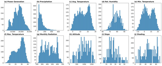
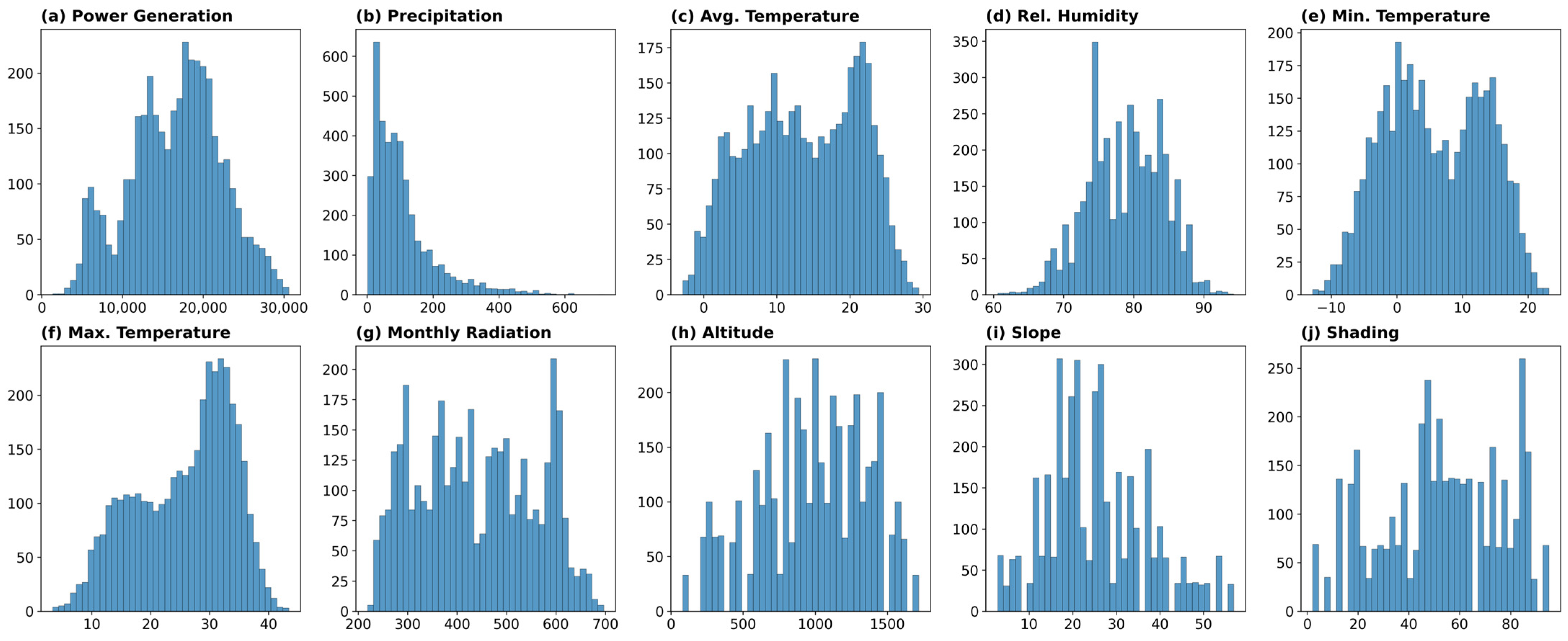
The distributions of the target variable and predictors after quality control are shown in Figure 11. Monthly generation is mainly concentrated between approximately 10,000 and 25,000 kWh, reflecting both the seasonal cycle and station-level differences. Meteorological variables show clear seasonal variability, while terrain indicators such as elevation, slope, and shading ratio represent fixed station-level spatial attributes.
Figure 11.
Distributions of monthly generation, meteorological variables, and terrain variables used in the modeling framework.
To characterize the topographic variability represented by the sample, summary statistics of the station terrain attributes are reported in Table 6. The 118 stations span a wide terrain range, with elevations from 80 to 1717 m (median 1015 m), slopes from 2.8 to 56.9° (median 24.7°), and terrain-shading ratios from 2 to 95% (median 53%). This confirms that the sample covers substantial topographic diversity, so the weak direct correlation between terrain indicators and monthly generation reflects a property of the already-sited stations rather than a lack of terrain variability in the sample.
Table 6.
Summary statistics of the terrain attributes of the 118 mountain PV stations (one value per station).
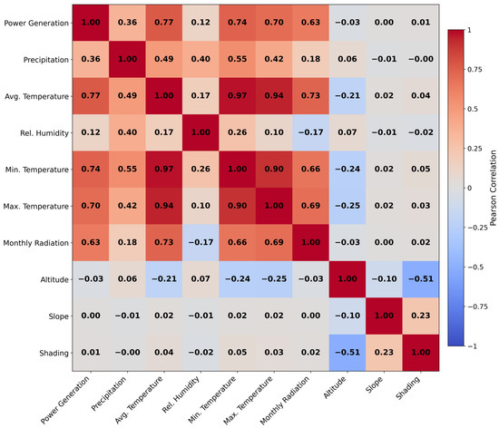
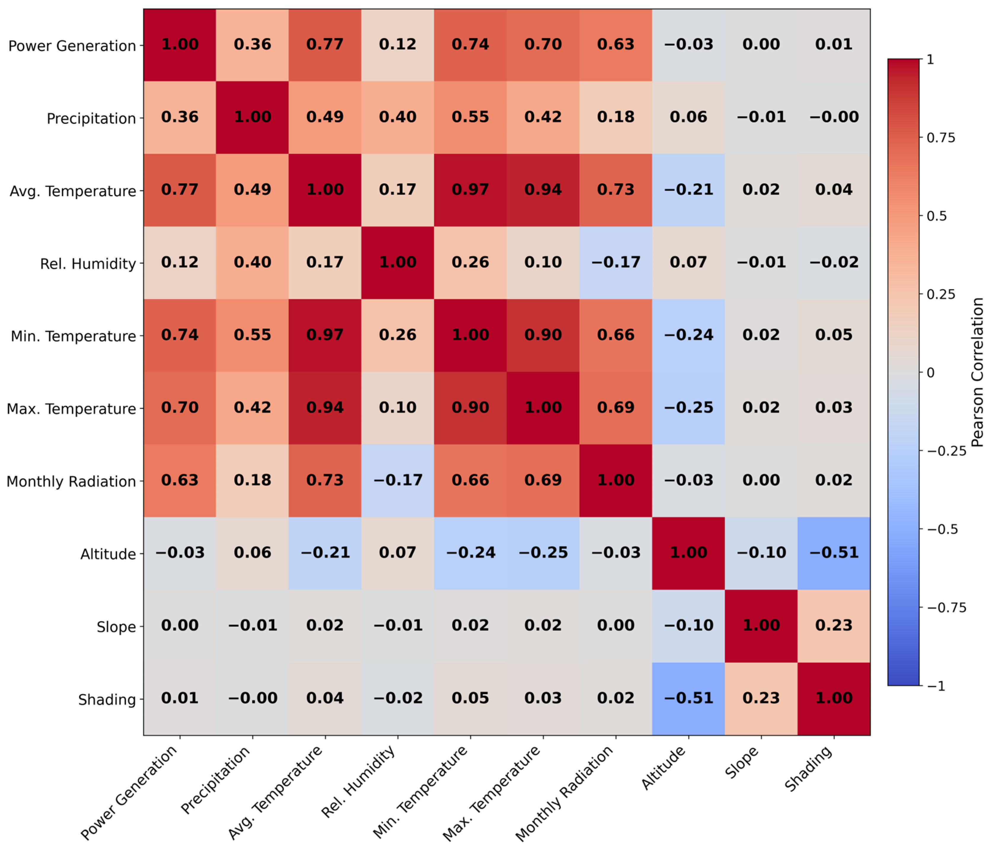
The Pearson correlation heatmap shows that monthly generation is most strongly correlated with temperature-related variables and monthly radiation (Figure 12). The Pearson correlation coefficients between generation and average temperature, minimum temperature, maximum temperature, and monthly radiation are 0.77, 0.74, 0.70, and 0.63, respectively. In contrast, the direct correlations between generation and terrain indicators are weak, with correlation coefficients of −0.03 for elevation, approximately 0 for slope, and 0.01 for shading ratio.
Figure 12.
Pearson correlation heatmap among monthly generation, meteorological variables, and terrain variables.
Although precipitation shows a positive Pearson correlation with monthly generation (r = 0.356), this relationship almost disappears after controlling for monthly radiation and average temperature (partial r = 0.010, p = 0.524). Therefore, the positive precipitation-generation correlation mainly reflects seasonal covariation rather than a direct causal promoting effect of precipitation on PV generation. Average, minimum, and maximum temperature are highly correlated, with pairwise correlation coefficients of 0.975, 0.941, and 0.901. Therefore, their individual importance values should not be interpreted as independent physical contributions. In the revised analysis, these variables are interpreted as a temperature-related variable group.
3.5. Feature Importance and Driving Factors
Feature-importance values from different models should be interpreted cautiously because different algorithms use different importance definitions and because several predictors are strongly correlated. Therefore, the revised analysis emphasizes grouped interpretation rather than exact percentages for individual variables.
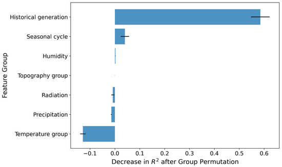
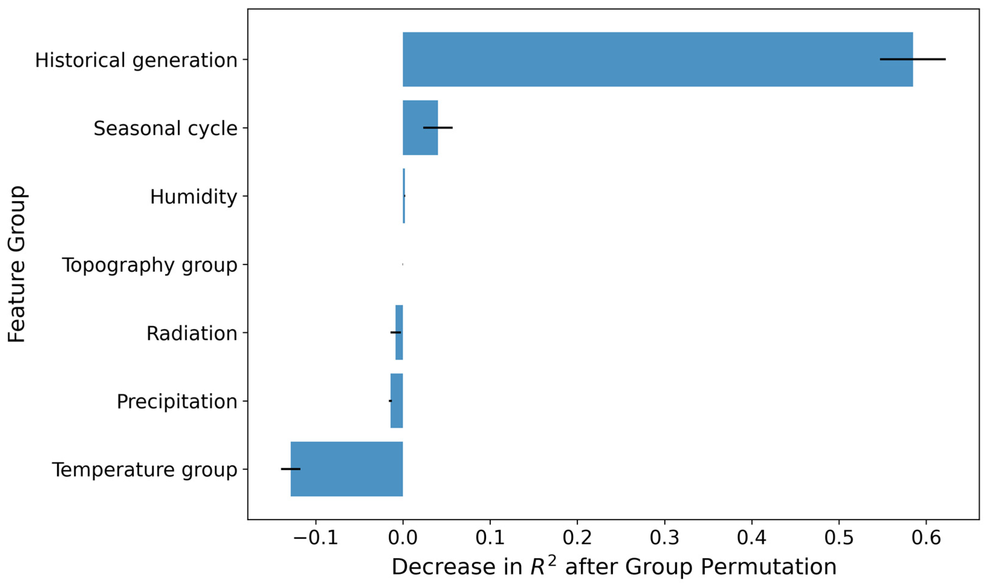
Grouped permutation importance based on the strict 2021 temporal validation indicates that historical-generation features are the most influential predictor group for the best temporal-validation model, followed by the seasonal-cycle variables. The near-zero or negative permutation importance of some meteorological groups should not be interpreted as evidence that these physical factors are unimportant. Instead, it indicates that, under the short training period and strict cross-year validation, the model relies strongly on historical generation and seasonal information, while the independent contribution of highly correlated meteorological variables is less stable. Therefore, grouped permutation importance is used here mainly as a diagnostic tool rather than a strict causal ranking of physical drivers.
As shown in Figure 13, historical-generation features produced the largest positive decrease in R2 after permutation, confirming that station-specific historical generation information was the dominant predictor group under the strict chronological validation. Seasonal-cycle variables also contributed positively. In contrast, several meteorological groups showed near-zero or negative grouped permutation importance, which should be interpreted cautiously because these variables are strongly correlated with seasonal-cycle and historical-generation features.
Figure 13.
Grouped permutation importance of CatBoost based on the independent 2021 validation period. The decrease in R2 after group permutation represents the contribution of each feature group to model performance. Error bars indicate variability across repeated permutations.
3.6. Annual-Generation Uncertainty Estimation
To quantify the uncertainty of annual energy yield, residual bootstrapping was applied to the best temporal-validation model. Monthly validation residuals were resampled and added to the predicted monthly generation values to generate an ensemble of possible monthly outcomes. These monthly samples were then aggregated to the annual scale for each station, and the 5th and 95th percentiles were used as the annual 90% prediction interval.
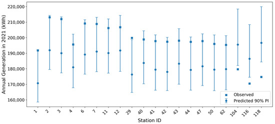
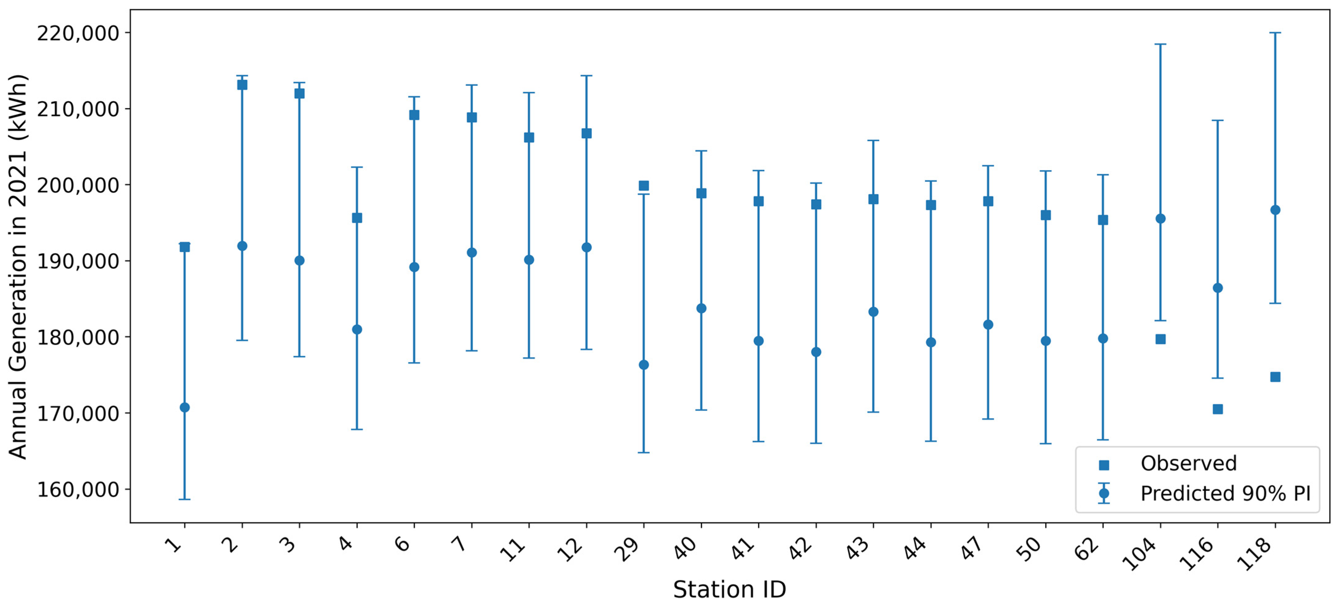
Using CatBoost as the reference model, the annual 90% prediction interval achieved an empirical coverage of 94.9% across the 118 stations, with a mean interval width of approximately 35,082 kWh. This result indicates that the residual-bootstrap interval provides a relatively conservative estimate of annual-generation uncertainty. However, the relatively wide interval also shows that monthly-to-annual generation prediction remains uncertain when only short historical records are available. Figure 14 illustrates the annual prediction intervals for representative stations and compares the interval estimates with observed annual generation in 2021.
Figure 14.
Annual generation prediction intervals for representative stations based on the CatBoost model. Error bars indicate the 90% prediction intervals, and square markers indicate observed annual generation in 2021.
The observed annual generation values of most representative stations fall within or close to the estimated 90% prediction intervals, supporting the use of residual bootstrapping as a practical uncertainty-quantification approach for monthly-to-annual PV generation assessment.
4. Discussion
The revised validation results show that the apparent model skill depends strongly on the validation design. Under the strict chronological split, CatBoost achieved the best temporal-validation performance, but the improvement over the monthly climatology baseline was limited. This indicates that monthly PV generation in 2021 contained interannual or operational variations that were not fully represented by the available meteorological, topographic, seasonal, and historical-generation predictors. In contrast, station-exclusion spatial cross-validation yielded substantially higher R2 values, with XGBoost, LightGBM, Random Forest, and CatBoost all performing well. This contrast suggests that, for the present three-year dataset, spatial transferability among already-built stations is stronger than cross-year extrapolation.
Although the chronological-validation R2 is modest and the improvement over the monthly climatology baseline is not statistically significant, the practical value of the proposed framework lies less in single-year point accuracy than in its spatial transferability to unseen stations (Section 3.3) and in the calibrated annual prediction intervals it provides for operational planning (Section 3.6). For medium-term distributed-PV assessment, a transferable model with quantified uncertainty is often more useful than a marginally higher single-year R2.
The dominance of radiation, temperature-related variables, seasonal cycle, and historical-generation features is physically reasonable. This joint use of meteorological and historical-generation predictors is consistent with recent medium-term PV forecasting studies [24], and the strong performance of gradient-boosted trees agrees with comparative evaluations of boosting and deep-learning models [25]. Monthly radiation controls the incident solar energy available for conversion, while temperature-related variables module thermal effects [26]. However, average, minimum, and maximum temperature are strongly collinear, and their individual importance values should not be interpreted as independent physical contributions. In this study, they are therefore interpreted as a temperature-related variable group.
The positive Pearson correlation between precipitation and generation should also be interpreted cautiously. After controlling for monthly radiation and average temperature, the precipitation-generation partial correlation becomes very weak and statistically insignificant. This indicates that the apparent positive precipitation correlation mainly reflects seasonal co-variation rather than a direct beneficial effect of precipitation on PV generation.
The weak direct contribution of terrain indicators should be interpreted carefully. The study area has strong relief, and the 118 stations cover a wide range of elevation, slope, aspect, and shading ratio. However, these are already-built village-level PV stations, and the original engineering siting process likely avoided extremely unfavorable valleys, severe terrain obstruction, unstable slopes, and inaccessible locations. Therefore, the constructed-station sample does not represent random terrain conditions across the county. The weak direct statistical relationship between terrain variables and monthly generation should be understood as a property of already-sited stations, not as evidence that terrain is unimportant for greenfield PV planning.
DEM resolution can influence the estimation of slope, aspect, and terrain-shading indicators. A coarse DEM may smooth local terrain features and underestimate obstruction in narrow valleys or steep terrain, whereas a high-resolution DEM can better capture local relief but may also introduce sensitivity to small-scale terrain noise and increase computational cost. The 25 m DEM used in this study provides a practical compromise for regional analysis [27]. Nevertheless, the shading ratio derived here should be interpreted as a terrain-scale obstruction metric, and future studies should compare 10 m, 25 m, and 30 m DEM products to quantify the sensitivity of PV-potential estimates to DEM resolution.
The monthly time step is suitable for medium-term generation assessment and operational planning, but it cannot resolve short-duration cloud variability, hourly terrain shading, transient precipitation events, inverter clipping, curtailment, or near-field shading. Hourly or sub-hourly simulations are more appropriate for analyzing shading events and operational dispatch. In addition, data-driven models depend strongly on the representativeness of historical records and may have limited extrapolation ability under unseen climate or operational conditions. They also cannot explicitly represent module degradation, cleaning, soiling, faults, curtailment, or near-field obstruction unless such variables are available. Therefore, the proposed framework should be regarded as a monthly generation forecasting and assessment tool for already-built stations rather than a full physical simulation or a complete greenfield site-selection model.
5. Conclusions
This study developed a multi-source framework for monthly generation forecasting of 118 standardized village-level mountain PV stations by integrating GHI-related solar-resource data, gridded meteorological variables, DEM-derived terrain indicators, viewshed-based terrain obstruction, seasonal-cycle variables, and historical-generation features.
(1) The 118 stations showed clear seasonal generation variability and moderate station-to-station differences. Based on three-year mean annual utilization hours, most stations were classified as General or Moderate, with an average annual utilization hour value of 916.7 h.
(2) Under strict chronological validation, CatBoost achieved the best temporal validation performance (R2 = 0.3119, MAE = 2719.7 kWh, RMSE = 3245.6 kWh), but its improvement over the monthly climatology baseline was limited. This indicates that cross-year extrapolation remains challenging when only two years of training records are available.
(3) Station-exclusion spatial cross-validation showed stronger transferability, with XGBoost achieving the highest mean R2 of 0.8659. This suggests that tree-based models can transfer well to unseen stations under similar multi-year climate and operational conditions.
(4) Temperature-related variables, monthly radiation, seasonal cycle, and historical-generation features were the major sources of predictive information. Terrain indicators showed weak direct correlations with monthly generation for already-sited stations, probably because engineering site selection had already filtered out extremely unfavorable terrain conditions. Therefore, the framework is most suitable for monthly generation forecasting and operational assessment of existing mountain PV stations, while greenfield site selection requires additional engineering, land-use, grid-access, and near-field shading information.
Author Contributions
Conceptualization, P.S. and D.M.; methodology, P.S. and D.M.; software, P.S.; validation, P.S., Y.X. and C.C.; formal analysis, P.S.; investigation, P.S. and M.W.; resources, M.W.; data curation, P.S. and Y.X.; writing—original draft preparation, P.S.; writing—review and editing, D.M., Y.X. and W.J.; visualization, P.S. and C.C.; supervision, M.W.; project administration, M.W. and W.J. All authors have read and agreed to the published version of the manuscript.
Funding
This work was supported by the China Meteorological Administration Key Open Laboratory of Transforming Climate Resource to Economy (No. 2025004K) and the Joint Research Project for Meteorological Capacity Improvement (No. 24NLTSQ017).
Institutional Review Board Statement
Not applicable.
Informed Consent Statement
Not applicable.
Data Availability Statement
The solar radiation data used in this study are publicly available from the Solargis database (https://solargis.com/ (accessed on accessed on 15 May 2026)). The meteorological data were obtained from the China Meteorological Administration Land Data Assimilation System (CLDAS-V2.0) and are available upon request. The DEM data are publicly available from NASA’s ASTER GDEM (https://lpdaac.usgs.gov/products/astgtmv003/ (accessed on 15 May 2026)). The measured PV generation data used in this study are not publicly available because they contain station-level operational information, but processed data and code may be made available from the corresponding author upon reasonable request, subject to data-use restrictions.
Acknowledgments
The authors thank the Solargis platform and the China Meteorological Administration for data support, and the data providers and station operators for supporting the PV generation and geospatial data collection.
Conflicts of Interest
The authors declare no conflicts of interest.
Abbreviations
The following abbreviations are used in this manuscript:
| Abbreviation | Full Name |
| PV | Photovoltaic |
| RF | Random Forest |
| LightGBM | Light Gradient Boosting Machine |
| XGBoost | Extreme Gradient Boosting |
| CatBoost | Categorical Boosting |
| MAE | Mean Absolute Error |
| RMSE | Root Mean Square Error |
| DEM | Digital Elevation Model |
| GHI | Global Horizontal Irradiance |
| MAD | Median Absolute Deviation |
| NWP | Numerical Weather Prediction |
| CLDAS | China Meteorological Administration Land Data Assimilation System |
| GDEM | Global Digital Elevation Model |
| SHAP | SHapley Additive exPlanations |
| SR | Shading Ratio |
References
- Yao, W.; Yue, C.; Xu, A.; Kong, X.; Cao, W.; Zheng, Z.; Yue, Q. Power generation evaluation of solar photovoltaic systems using radiation frequency distribution. J. Build. Eng. 2024, 98, 110981. [Google Scholar] [CrossRef] [Scilit]
- Han, B.; Xie, H.; Sui, J.; Shan, Y.; Chen, M.; Li, Y. Anomaly data detection algorithm of small photovoltaic power station based on machine learning. In Proceedings of the International Conference on Artificial Intelligence and Intelligent Information Processing (AIIIP 2022), Qingdao, China, 28–30 October 2022. [Google Scholar] [CrossRef] [Scilit]
- Xia, C.; Kong, C.; Zhao, J.; Zhang, L. Optimized configuration of energy storage in solar thermal power station considering solar multiple. In Proceedings of the 2024 6th International Conference on Energy, Power and Grid (ICEPG), Guangzhou, China, 27–29 September 2024. [Google Scholar] [CrossRef] [Scilit]
- Di Leo, P.; Ciocia, A.; Malgaroli, G.; Spertino, F. Advancements and challenges in photovoltaic power forecasting: A comprehensive review. Energies 2025, 18, 2108. [Google Scholar] [CrossRef] [Scilit]
- Al-Dahidi, S.; Madhiarasan, M.; Al-Ghussain, L.; Abubaker, A.M.; Ahmad, A.D.; Alrbai, M.; Aghaei, M.; Alahmer, H.; Alahmer, A.; Zio, E.; et al. Forecasting solar photovoltaic power production: A comprehensive review and innovative data-driven modeling framework. Energies 2024, 17, 4145. [Google Scholar] [CrossRef] [Scilit]
- Chakraborty, D.; Mondal, J.; Barua, H.B.; Bhattacharjee, A. Computational solar energy: Ensemble learning methods for prediction of solar power generation based on meteorological parameters in Eastern India. Renew. Energy Focus 2023, 44, 277–294. [Google Scholar] [CrossRef] [Scilit]
- Madan, C. An extensive review of recent development of solar power prediction models. J. Comput. Mech. Power Syst. Control 2025, 8, 34–42. [Google Scholar] [CrossRef] [Scilit]
- Liu, Z.; Guo, J.; Wang, X.; Wang, Y.; Li, W.; Wang, X.; Fan, Y.; Wang, W. Prediction of long-term photovoltaic power generation in the context of climate change. Renew. Energy 2024, 235, 121263. [Google Scholar] [CrossRef] [Scilit]
- Breiman, L. Random forests. Mach. Learn. 2001, 45, 5–32. [Google Scholar] [CrossRef] [Scilit]
- Ke, G.; Meng, Q.; Finley, T.; Wang, T.; Chen, W.; Ma, W.; Ye, Q.; Liu, T.-Y. LightGBM: A highly efficient gradient boosting decision tree. Adv. Neural Inf. Process. Syst. 2017, 30, 3146–3154. [Google Scholar]
- Chen, T.; Guestrin, C. XGBoost: A scalable tree boosting system. In Proceedings of the 22nd ACM SIGKDD International Conference on Knowledge Discovery and Data Mining (KDD ‘16), San Francisco, CA, USA, 13–17 August 2016; ACM: New York, NY, USA, 2016; pp. 785–794. [Google Scholar] [CrossRef] [Scilit]
- Prokhorenkova, L.; Gusev, G.; Vorobev, A.; Dorogush, A.V.; Gulin, A. CatBoost: Unbiased boosting with categorical features. Adv. Neural Inf. Process. Syst. 2018, 31, 6639–6649. [Google Scholar]
- Lundberg, S.M.; Lee, S.-I. A unified approach to interpreting model predictions. Adv. Neural Inf. Process. Syst. 2017, 30, 4765–4774. [Google Scholar]
- Vaswani, A.; Shazeer, N.; Parmar, N.; Uszkoreit, J.; Jones, L.; Gomez, A.N.; Kaiser, Ł.; Polosukhin, I. Attention is all you need. Adv. Neural Inf. Process. Syst. 2017, 30, 5998–6008. [Google Scholar]
- Alay, F.D.; İlhan, N.; Güllüoğlu, M.T. Solar radiation prediction in PV power systems: A comparison of deep learning models using big data. Proc. Bulg. Acad. Sci. 2024, 77, 1347–1354. [Google Scholar] [CrossRef] [Scilit]
- Deng, S.; Li, Y.; Zhang, J.; Yang, L.; Cai, Z.; Wu, B. Power prediction of regional photovoltaic power stations based on meteorological encryption and spatio-temporal graph networks. Energies 2024, 17, 3557. [Google Scholar] [CrossRef] [Scilit]
- Feng, X.; Zhang, Z.; Chen, Q.; Guo, Z.; Zhang, H.; Wang, M.; Gao, W.; Liu, X. Integrating remote sensing, GIS, and multi-criteria decision making for assessing PV potential in mountainous regions. Renew. Energy 2025, 241, 122340. [Google Scholar] [CrossRef] [Scilit]
- Zhang, J.; Fu, S.; Tao, J.; Han, Q.; Wang, Y.; Ge, Y.; Li, Z.; Zhong, Y.; Yan, B. Climate environmental impact analysis of a mountain photovoltaic plant. Sol. Energy 2024, 282, 112930. [Google Scholar] [CrossRef] [Scilit]
- Zhang, W. Prediction and influencing factors of photovoltaic system power generation of a single house based on continuously measured data. Indoor Built Environ. 2023, 33, 195–210. [Google Scholar] [CrossRef] [Scilit]
- Peng, H.; Xiong, Y.; Abuduwayiti, X. Data-driven characterization of photovoltaic power generation under multi-factor coupling effects. J. Phys. Conf. Ser. 2025, 3079, 012035. [Google Scholar] [CrossRef] [Scilit]
- NASA/METI/AIST/Japan Spacesystems and U.S./Japan ASTER Science Team. ASTER Global Digital Elevation Model V003 [Data Set]; NASA EOSDIS Land Processes Distributed Active Archive Center: Sioux Falls, SD, USA, 2019. [CrossRef] [Scilit]
- Han, S.; Liu, B.; Shi, C.; Liu, Y.; Qiu, M.; Sun, S. Evaluation of CLDAS and GLDAS datasets for near-surface air temperature over major land areas of China. Sustainability 2020, 12, 4311. [Google Scholar] [CrossRef] [Scilit]
- IEC 61724-1:2021; Photovoltaic System Performance—Part 1: Monitoring. NSAI Standard: Dublin, Ireland, 2017.
- Yang, Y.; Lee, S.-H.; Choi, Y.-S.; Lee, K.-M. LightGBM medium-term photovoltaic power prediction integrating meteorological features and historical data. Energies 2025, 18, 5526. [Google Scholar] [CrossRef] [Scilit]
- Vargas, J.; Martínez, R.; Loo, L. Enhancing Photovoltaic Energy Forecasting with Machine Learning: A Comparison Study of XGBoost, LightGBM and LSTM Models. In Proceedings of the 2024 IEEE Latin American Conference on Computational Intelligence (LA-CCI), Bogotá, Colombia, 13–15 November 2024; pp. 1–6. [Google Scholar] [CrossRef] [Scilit]
- Skoplaki, E.; Palyvos, J.A. On the temperature dependence of photovoltaic module electrical performance: A review of efficiency/power correlations. Sol. Energy 2009, 83, 614–624. [Google Scholar] [CrossRef] [Scilit]
- Heo, J.; Jung, J.; Kim, B.; Han, S. Digital elevation model-based convolutional neural network modeling for searching of high solar energy regions. Appl. Energy 2020, 262, 114588. [Google Scholar] [CrossRef] [Scilit]

Disclaimer/Publisher’s Note: The statements, opinions and data contained in all publications are solely those of the individual author(s) and contributor(s) and not of MDPI and/or the editor(s). MDPI and/or the editor(s) disclaim responsibility for any injury to people or property resulting from any ideas, methods, instructions or products referred to in the content. |
© 2026 by the authors. Licensee MDPI, Basel, Switzerland. This article is an open access article distributed under the terms and conditions of the Creative Commons Attribution (CC BY) license.