


Abstract
To overcome the computational bottlenecks of iterative Computational Fluid Dynamics (CFD) in turbomachinery design, this study introduces a real-time, data-driven inverse design framework for 2D uncooled, high-Reynolds turbine blades. The novelty of this work lies in the application of Kolmogorov–Arnold Networks (KAN), a distinct deep-learning architecture, to predict blade geometry and performance metrics from aerodynamic loading inputs. The foundation of the model is a comprehensive database of approximately 30,000 blade profiles, generated through an automated optimization pipeline coupled with the MISES solver. This dataset explores an extensive design space, covering inlet flow angles from to and outlet angles from to , with flow turning up to . A rigorous benchmarking campaign compares KAN against Multi-Layer Perceptrons (MLPs) and Gaussian Process Regression (GPR), highlighting KAN’s capability to overcome the scalability bottlenecks of Gaussian Process Regression to enable real-time performance while achieving MLP-level accuracy with significantly fewer parameters. A further analysis regarding the trade-off between database size and filtration of unfeasible designs indicates that an optimal data filtration threshold exists, balancing noise reduction with model robustness. The final KAN tool achieves real-time inference speeds (∼0.1 s), reducing the design cycle by four orders of magnitude compared to traditional solvers, while maintaining high accuracy (mean outlet angle error of and Mach profile RMS error of ). Furthermore, the model’s predicted RMS error is exploited as a quantitative proxy for aerodynamic feasibility, identifying ill-posed inverse problems where the target loading cannot be physically realized. This metric enables the generation of comprehensive maps that rigorously delineate the boundaries of the viable design space across arbitrary aerodynamic loading styles, providing physics-aware guidelines for preliminary design.
1. Introduction
Traditional turbomachinery design workflows typically rely on direct optimization approaches, where designers iteratively refine blade geometries through CFD simulations and empirical heuristics. Although effective, this process is inherently slow, computationally expensive, and heavily dependent on designer experience and intuition. In many cases, early-stage designs neglect crucial physical phenomena, such as tip leakage, three-dimensional flow structures, boundary-layer interactions, and shock/boundary-layer separations, that can only be accurately captured in later design stages. As a result, multiple geometry iterations are often required even in preliminary phases, making redesign costly in time and computational resources. In recent years, it has become increasingly evident that the accurate prediction of aerodynamic quantities and flow-field characteristics from the earliest design stages is essential to accelerate innovation in turbomachinery. Early-phase prediction enables wide exploration of the design space while maintaining physical consistency, allowing designers to assess the aerodynamic feasibility of new concepts before committing to expensive CFD campaigns. In this context, several studies have explored the integration of machine learning (ML) and artificial intelligence (AI) into aerodynamic design processes. Building on foundational work coupling neural networks with Navier–Stokes solvers [1,2], recent research has leveraged deep learning to enhance shape optimization and performance prediction loops [3,4,5,6,7]. These methodologies have extended beyond 2D profiling to address complex 3D features such as tip leakage flows [8,9], while Graph Neural Networks and data-centric approaches have been employed to reconstruct flow fields and provide deeper physical insights into loss mechanisms [10,11]. Clark [12] introduced an inverse design system based on radial basis function networks. His method established a continuous mapping between aerodynamic duty, style, and resulting geometry, enabling fast and accurate profile generation with orders-of-magnitude computational savings. Building on this concept, Bellucci et al. [13] developed an advanced AI-assisted optimization environment for low-pressure turbines, combining automated CFD-database generation with ANN-based surrogate modeling. Their framework directly incorporated unsteady effects in the optimization loop and achieved real-time prediction of aerodynamic performance and flow fields. Similarly, Petronio et al. [14] integrated Gaussian Process Regression with Proper Orthogonal Decomposition (POD) to identify minimum-loss design regions in low-pressure turbines. This physics-informed surrogate model efficiently explored the design space by selecting the most informative samples, reducing the number of required CFD simulations while maintaining high accuracy in predicting losses and blade loading. Zou et al. [15] proposed a two-stage hybrid model combining deep learning with multi-output Gaussian Processes (MOGPs). The employment of a dual-network approach enabled the automatic determination of optimal turbine geometries without iterative optimization, further demonstrating the potential of ML models to accelerate turbomachinery design. Despite these advances, several key challenges remain before data-driven methodologies can be adopted in turbomachinery design with the requisite reliability and consistency. Existing literature often lacks a systematic procedure for the end-to-end construction, training, and validation of AI-based design tools, specifically regarding the rigorous selection of the training database. There is a notable gap in understanding the trade-off between cleaning the dataset of unfeasible designs (noise reduction) and maintaining a sufficiently broad design space for generalization. Second, while surrogate modeling is common, the literature lacks a rigorous comparative assessment of different model architectures, leaving the specific trade-offs between complexity, accuracy, and efficiency largely unexplored. To address these gaps, the present work introduces a comprehensive, AI-powered framework for turbomachinery design that systematically integrates database generation, model training, and data-driven analysis. Expanding upon the design space definition proposed by Clark [12], this study enlarges the geometric bounds to cover a wider range of aerodynamic duties. The primary contribution of this work is the definition of a complete, end-to-end framework for the generation of such data-driven design tools. A comprehensive database of 30.000 airfoil shapes was built, each targeting a specific combination of aerodynamic duty and blade loading distribution, designed with a MISES-coupled shape optimization. In this automated workflow, the solver iteratively evaluates and refines candidate profiles to achieve the targeted pressure distributions. As demonstrated by recent state-of-the-art methodologies for large-scale dataset generation [11,16], MISES is highly effective for this task. For 2D blade sections operating in regimes where gross flow separation and complex transition modeling are not dominant, its coupled viscous-inviscid formulation yields aerodynamically resolved data comparable in accuracy to steady RANS, while offering a 2–3 order-of-magnitude reduction in computational time. Within this framework, we conducted a dedicated analysis of the training database composition. We provide specific insights regarding the optimal selection of data, addressing the critical trade-off between the filtration of extreme, unfeasible points and the preservation of prediction capabilities over a large design space. Furthermore, this study explicitly benchmarks Gaussian Process Regression (GPR), Multi-Layer Perceptrons (MLPs), and Kolmogorov–Arnold Networks (KAN), directly quantifying their respective performance to identify the most efficient predictor. Finally, the trained models are utilized not merely as predictive surrogates but as analytical instruments. The model’s predicted RMS error is exploited as a quantitative proxy for aerodynamic feasibility, identifying ill-posed inverse problems where the target loading cannot be physically realized. This metric enables the generation of comprehensive maps that rigorously delineate the boundaries of the viable design space across arbitrary aerodynamic loading styles, providing physics-aware guidelines for preliminary design and enabling the extraction of meaningful correlations between geometric features, aerodynamic duty, and flow characteristics.
2. Prior Knowledge Generation
This section details the methodology for generating the high-Re 2D uncooled blade database, focusing on the optimization strategy, parametrization, and critical configuration parameters. The automated workflow comprises four key components:
- Blade geometry parametrization;
- Target features definition;
- Flow computation and post-processing;
- Optimization strategies and database creation.
2.1. Design and Parametrization of Turbine Blade Passages
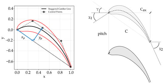
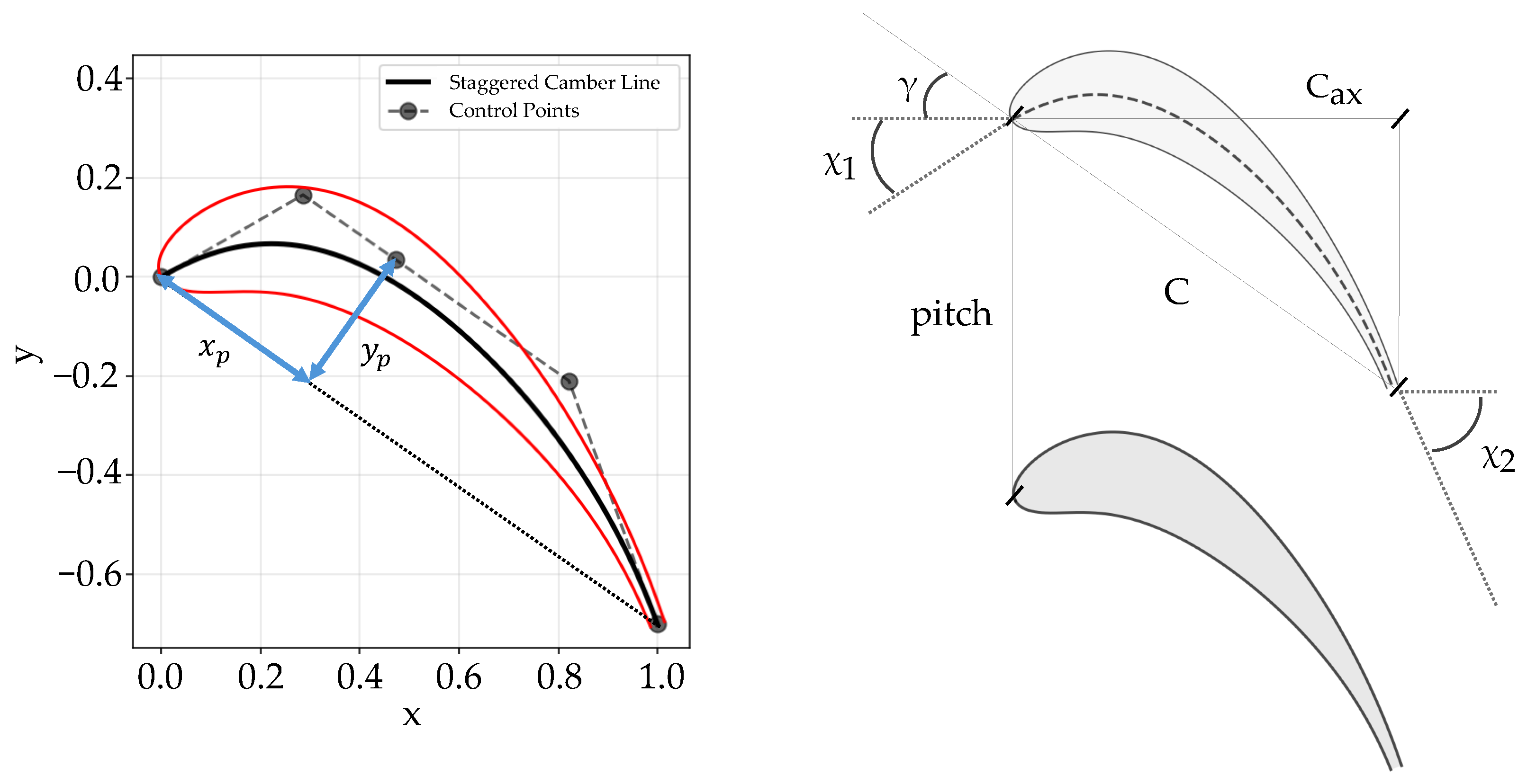
Blade geometry parametrization must balance flexibility for arbitrary shapes with minimal dimensionality. The chosen approach leverages the “shape space” concept by Kulfan [17,18,19], utilizing a novel fourth order B-spline camber line defined by five parameters: inlet () and outlet () metal angles, peak curvature coordinates (), and stagger angle (). These parameters uniquely determine five control points (Figure 1), ensuring flexibility and robust control.
Figure 1.
Camber line parametrization through 4-th order B-spline using 5 control points.
The camber line formulation ensures a cohesive and continuous curve up to continuity, defined by Equation (1) as follows:
where the following apply:
- is the B-spline curve;
- is the B-spline basis function of degree p;
- are the control points;
- n is the number of control points minus 1.
Thickness distribution () along the normalized chord () is superimposed onto the camber line to define pressure and suction sides. The thickness profile is a summation of n Bernstein polynomials with coefficients , scaled by a class function :
Coefficients and produce a round leading edge and pointed trailing edge, consistent with Kulfan’s method. The trailing edge thickness is fixed at . The leading edge radius () is controlled by (Equation (2)), which varies independently for pressure and suction sides to enhance geometric flexibility. The final profile coordinates are obtained by superimposing thickness onto the camber line (Equation (4)):
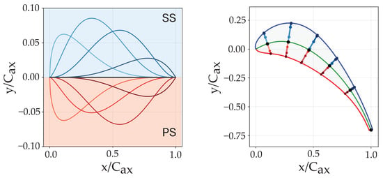
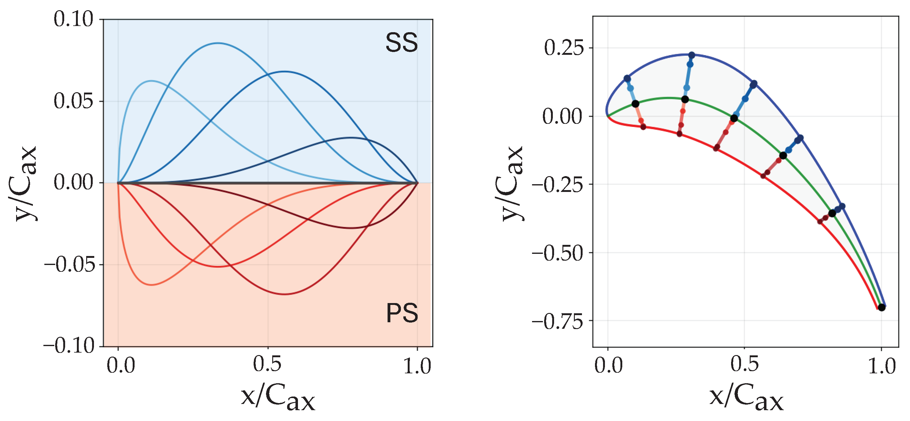
Employing Kulfan’s approach ensures the reproduction of high-quality airfoil shapes, characterized by smooth derivatives, and offers the flexibility to scale up the number of thickness components fluently. Figure 2 demonstrates the geometric variation achievable by modifying coefficients, confirming the method’s suitability for exploring extensive design spaces.
Figure 2.
Example of blade section, showing the camber line and the individual Kulfan’s components that define the final surface.
2.2. Target Features Definition
This section defines the target features and their design ranges. Each data point corresponds to a unique combination of aerodynamic duty and style. Aerodynamic duty specifies boundary conditions: inlet flow angle (), outlet flow angle (), and outlet Mach number (). The outlet Reynolds number is fixed at = 600,000, with the inlet axial Reynolds number () derived via conservation equations. Specific heat ratio and Axial Velocity Density Ratio () are constant at 1.4 and 1, respectively. Aerodynamic style defines the Mach number distribution along pressure and suction surfaces, parameterized by four variables.
The four design parameters are hereby listed below:
- : ratio between the peak Mach number on the suction side and ;
- : axial position of the peak Mach number on the suction side;
- : ratio between the leading edge pressure side Mach number and ;
- : ratio between the leading edge suction side Mach number and .
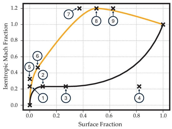
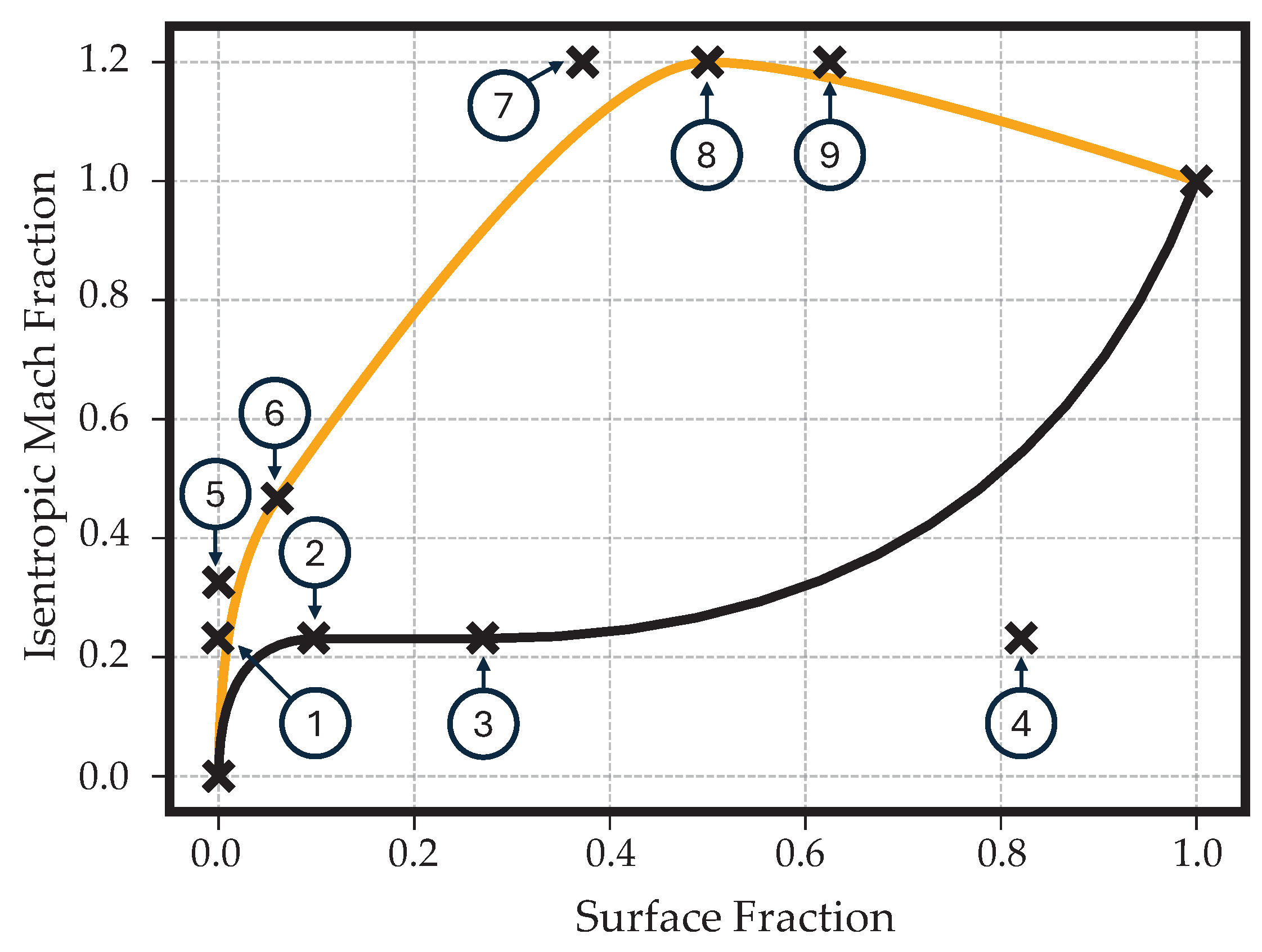
The surface isentropic Mach numbers are normalized by the trailing edge value, forming the isentropic Mach fraction (). The use of the non-dimensional surface length () as the independent variable allows for greater control over leading-edge loading and flow diffusion. The final distribution is built using linear functions and B-splines, ensuring smoothness. Control point placement (Figure 3) was optimized to maximize feasible loading distributions and therefore physical blade shapes.
Figure 3.
Loading parametrization with enumerated control points.
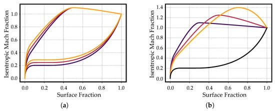
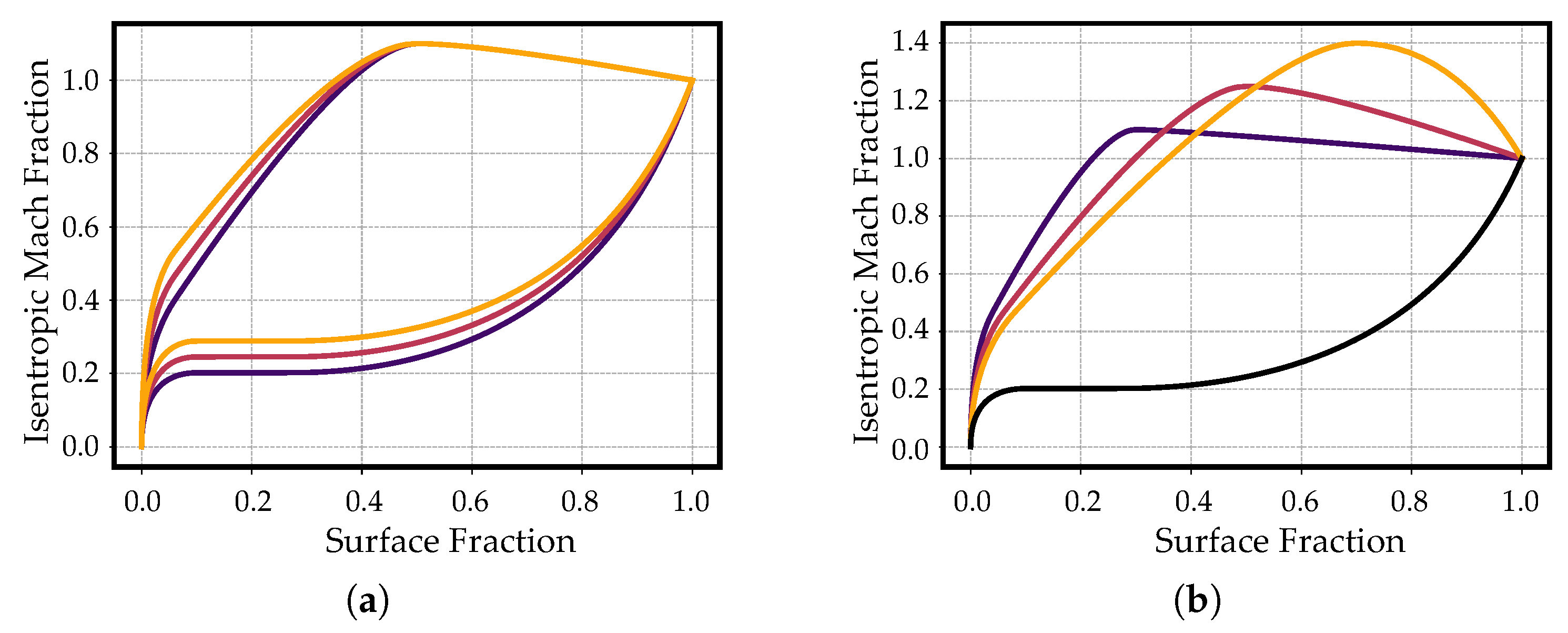
Suction side leading edge surface fraction (point 6) is 10% of , while the pressure side is fixed at 0.1. Control point 1 is fixed at () to enforce an infinite slope. Points 3 and 4 are fixed at fractions 0.27 and 0.82. Point 5 lies at the y-axis intercept of the line connecting points 6 and 7. Points 7 and 9 allow axial variation relative to while maintaining . Leading edge Mach numbers are normalized by inlet axial Mach () and inlet Mach () for pressure and suction sides, respectively, to maintain loading consistency as evolves during simulation, thereby altering the target isentropic Mach number distribution. Nevertheless, once the optimization approaches convergence, these variations will be negligible. Figure 4 illustrates generated Mach profiles. The optimization process iteratively minimizes the discrepancy between target and computed Mach distributions and outlet flow angles.
Figure 4.
Effect of variables variation on the isentropic Mach fraction distribution. Variation in and (a) and variation in and (b) variables within the design range specified in Table 1.
The selection of a blade-loading parametrization inherently constrains the inverse-design problem to a low-dimensional loading space. The implemented four-parameter formulation represents a deliberate compromise between aerodynamic flexibility, database generation cost, and model robustness. While this parametrization is highly representative of conventional mid-loaded and aft-loaded low-pressure turbine profiles, it cannot encapsulate all possible loading organizations. Specifically, it lacks the complexity to accurately reproduce low-reaction or impulse rotor profiles, as well as transonic or supersonic blade sections where shock waves and strong shock-boundary-layer interactions dictate more intricate surface Mach number distributions. Consequently, certain aerodynamic duties may register as infeasible within this framework, not due to physical impossibility, but because fulfilling them requires a loading organization outside the prescribed parametric bounds. Nevertheless, the underlying optimization framework remains independent. Modifying or extending the loading parametrization would simply redefine the accessible design space, allowing the optimizer to generate alternative blade geometries tailored to those new requirements.
2.3. Flow Simulation and Post-Processing
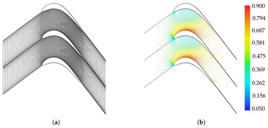
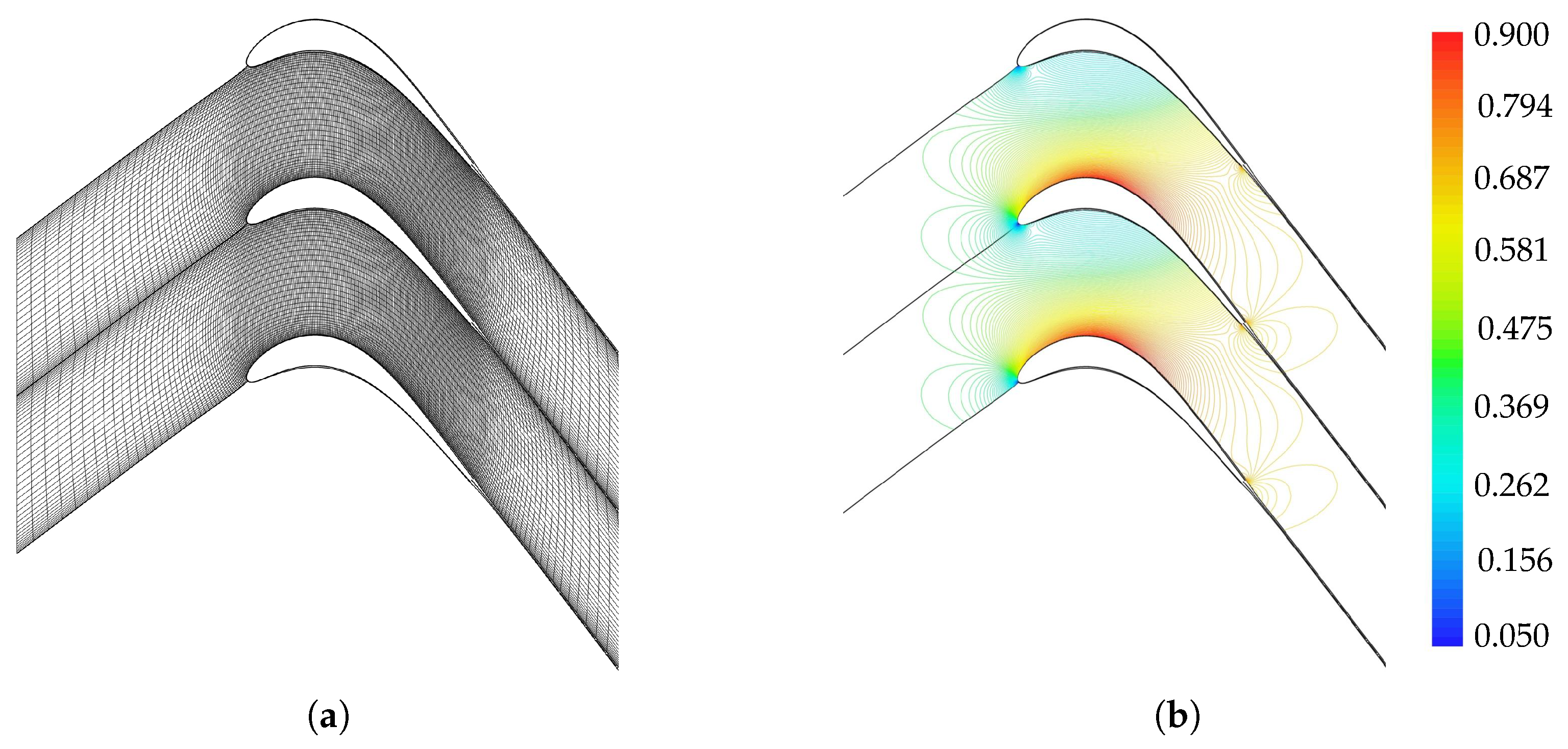
To obtain the aerodynamic output variables, namely the real flow angles and the real Mach distribution along the pressure and suction sides for every database point, a flow computation using MISES (Multiple blades Interacting Streamtube Euler Solver) [20,21,22] is performed. The automated workflow utilizes integrated modules to generate a hybrid H-type/O-type mesh (Figure 5) with 6000 cells, balancing computational speed with accuracy. To prevent the introduction of erroneous data, a final simulation for each data point using an I-type grid is done, as this has been demonstrated to possess greater stability properties. Boundary conditions are defined by inlet flow angle, inlet axial Reynolds number, and outlet Mach number. Turbulence intensity is fixed at 3.5%, with boundary layer tripping at 3% axial chord to ensure fully turbulent flow and simulation stability. The MISES solver was selected for this study due to its ability to achieve an accuracy comparable to fully resolved Reynolds-Averaged Navier–Stokes (RANS) simulations while reducing computational costs by two to three orders of magnitude. It is acknowledged that deploying a higher fidelity RANS solver would likely yield slight variations in the predicted flow field. This is primarily because MISES enforces a Kutta condition at a blunt trailing edge rather than explicitly resolving the complex wake physics. Consequently, an inherent limitation of this modeling approach is a tendency to underpredict wake-mixing losses and an inability to accurately capture the base pressure on the trailing edge. Despite these localized discrepancies, MISES remains a valuable design tool that enables the rapid evaluation and optimization of section geometries across a wide range of operating conditions.
Figure 5.
Example of mesh generation through the ISET module (a) and Mach number contour plot after flow simulation through the ISES module (b).
While higher-fidelity methods, such as Large Eddy Simulation (LES) or Direct Numerical Simulation (DNS), would strictly provide greater physical accuracy, their prohibitive computational expense renders them unfeasible for the extensive dataset generation required in the present framework.
2.4. Optimization Strategies and Database Creation
Database creation involves optimizing blade geometry to match specified aerodynamic style and duty. This section details the optimization procedure and resulting database characteristics.
2.4.1. Optimization Setup
A modified Nelder–Mead algorithm [23] is employed for shape tuning, selected for its gradient-free robustness against the ill-conditioned minimization function inherent to this problem. To mitigate slow convergence and local minima, a fine-tuned stage optimization strategy has been designed. Initially, the number of Kulfan’s modes for the pressure and suction side thickness is set to two in order to accelerate convergence by limiting the degrees of freedom, allowing also for a broader exploration of the design space with less probability of achieving unfeasible geometries. As the optimizer progresses, the DOFs are successively doubled to improve accuracy and obtain a more refined geometry. This procedure continues until a predefined acceptance threshold is satisfied or the maximum number of iterations is reached. Furthermore, an annealing operation is foreseen every 70 iterations along with the optimization. During this stage, the normalized design parameter values vary by adding a random number within the range multiplied by an annealing coefficient , which initial value is set to 1.
The coefficient is reduced by a factor of 0.95 every time annealing is performed, in order to guarantee a gradual convergence. Another meaningful aspect concerns the definition of the geometrical parameters boundaries throughout the optimization process. To ensure a broad exploration of the design space, the stagger angle limits were defined as the correlation-based initial value derived from Kacker and Okapuu [24], with an allowable variation of . The metal angle bounds permitted a deviation of from the aerodynamic duty inlet flow angle. The pitch-to-axial-chord ratio design region was constrained between 0.4 and 2.25, while the variation in Kulfan’s shape parameters was restricted to the range [0, 2.5]. The first coefficient is subjected to different constraints since it sets the leading edge radius value. The leading edge radius is constrained to the range , while the trailing edge value is set to 0.03. The Cartesian coordinates defining the peak curvature of the camber line, and , are varied within the ranges and , respectively. To ensure the generation of feasible airfoil shapes, the design parameter ranges were strictly bounded, together with a proper selection of the initial guess of the optimization vector, featuring and equal to respectively 0.3 and 0.6. Furthermore, non-converged MISES simulations, which generally indicate non-physical geometries, were automatically penalized with an artificially high cost to steer the optimizer away from unviable design regions. Each design parameter is normalized in order to enhance the robustness of the overall process. The cost function g, whose formulation was refined in accordance with Clark [12], is hereby proposed to be minimized:
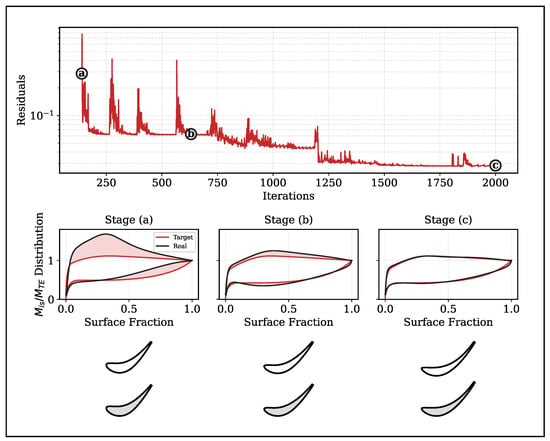
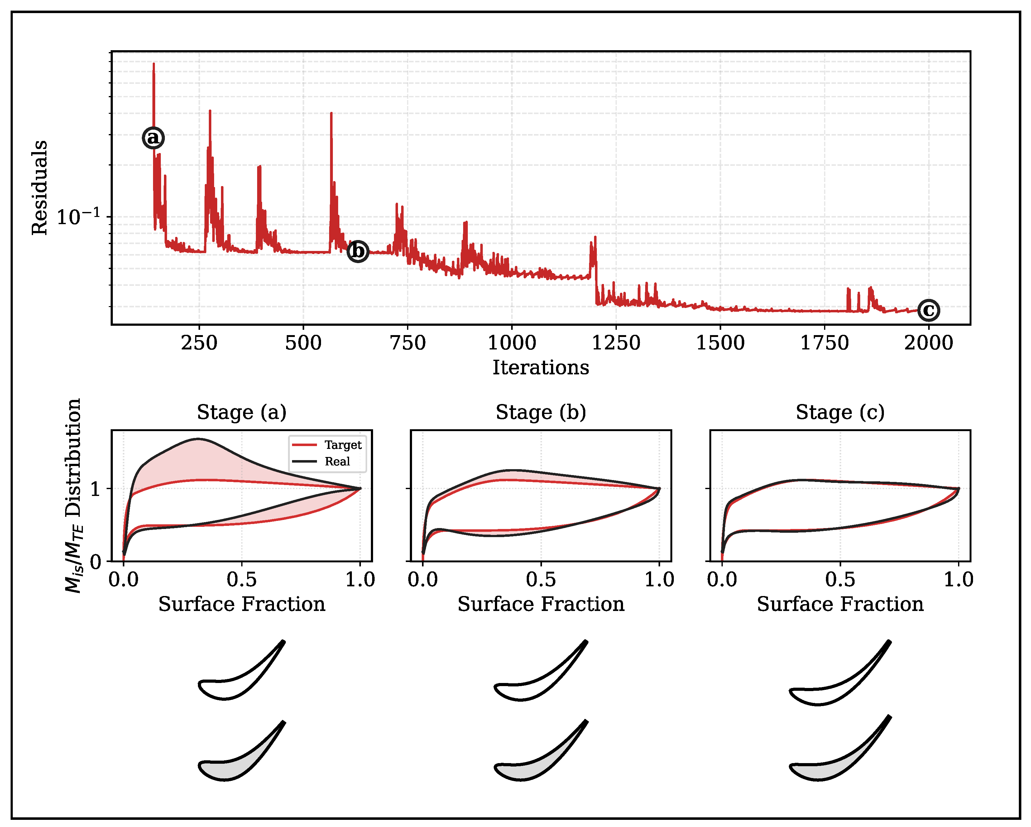
The cost function directs the optimization toward the desired solution by enforcing a match between the computed and target loading distributions and outlet flow angle. Empirical tests indicate that doubling the weight of the pressure-side loading in the early stages ensures the generation of realistic blade shapes. Prioritizing this feature significantly facilitates the subsequent convergence of the suction side and outlet flow angle. An example of this convergence behavior is shown in Figure 6, which illustrates the evolution of both the blade geometry and the corresponding loading distribution throughout the optimization process. The optimizer enforces convergence when the RMS error and flow angle deviation () fall below 0.01 and 0.1, respectively, or when the limit of 400 iterations, which resets each time Kulfan modes are doubled, is exhausted. Despite these strict thresholds, acceptable accuracy is typically observed once RMS values stabilize around 0.03–0.05.
Figure 6.
Optimization convergence overview. Top: History of the residual cost function. Bottom: Evolution of the aerodynamic loading distribution (middle row) and blade geometry (bottom row) corresponding to three key stages: (a) ∼100 iterations, (b) ∼600 iterations, and (c) 2000 iterations. The shaded regions highlight the discrepancy between the target (red) and actual (black) loading.
2.4.2. Database Results
Table 1 shows the ranges of the variables in the prior knowledge generation. A wider parameter range was selected with respect to Clark’s analysis [12], increasing the achievable flow turning up to and comprehending front-loaded blades. Each point in the database is described by a total of 43 parameters, with 36 representing Kulfan’s modes and the remaining 7 corresponding to the camber line parameters, pitch-to-chord ratio and trailing edge radius. It was chosen not to increase furthermore the number of Kulfan’s modes, considering the negligible geometrical and computational benefit. It is important to note that not all combinations of aerodynamic style and duty are viable. Consequently, significant residual costs persist in some designs, primarily driven by deviations from the target loading distribution. The total number of database points is 30.128, considering 128 corner points and 30.000 internal points sampled using a Latin HyperCube Sampling (LHS). This sampling strategy offers the advantage of selecting random variable values that are uniformly spread across their range while taking into account the probability density function of those random variables. The database creation process was initiated with the generation of 128 corner points, which delineated the boundaries of the design space. Subsequently, every internal point was initialized using a weighted interpolation of the nearest corner points to provide a robust starting guess and fasten convergence.
Table 1.
Ranges of variables for prior knowledge generation.
Following convergence, each sample is augmented with a comprehensive set of computed outputs. This includes aerodynamic results, such as the real outlet flow angle and isentropic Mach distributions, alongside post-processed geometric features like blade area, maximum thickness, chord, and suction side arc length. The kinetic energy loss coefficient is evaluated according to the formulation in Equation (7) [25], where the outlet pressures represent mass-flow averaged values corrected for mixing losses.
Divergence occurred in edge cases where the global simulation settings were incompatible with complex geometries, which required either specific meshing strategies or bespoke numerical adjustments to converge. After the exclusion of these cases, 29.972 data points remained for further analysis. Table 2 summarizes the database statistics, presenting the mean, standard deviation, and minimum/maximum values for both the root mean square (RMS) error and the outlet flow angle error.
Table 2.
Database points analysis.
All simulations were executed on a dual-socket AMD EPYC 7551 Linux machine. A single MISES simulation required approximately 0.5 s of wall-clock time on a single CPU core. A total of 128 cores were used in parallel for the database of 30.128 points creation over the course of 15 days.
3. Fast Machine Learning Tool
We present a machine-learning framework designed to predict the geometry and aerodynamics of 2D, uncooled, high-Reynolds-number blades. This surrogate model replaces computationally expensive simulations by learning the mapping between geometric parameters and key aerodynamic outputs. This capability allows for rapid design iteration and broad exploration of the design space.
3.1. KAN
Kolmogorov–Arnold Networks (KAN) [26,27] represent a novel approach to deep learning, offering a new method for constructing neural networks. This approach draws inspiration from the existing Kolmogorov–Arnold representation theorem, which states that every multivariate continuous function can be represented as a finite composition of continuous uni-variate functions and the binary operation of addition.
where and .
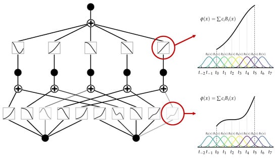
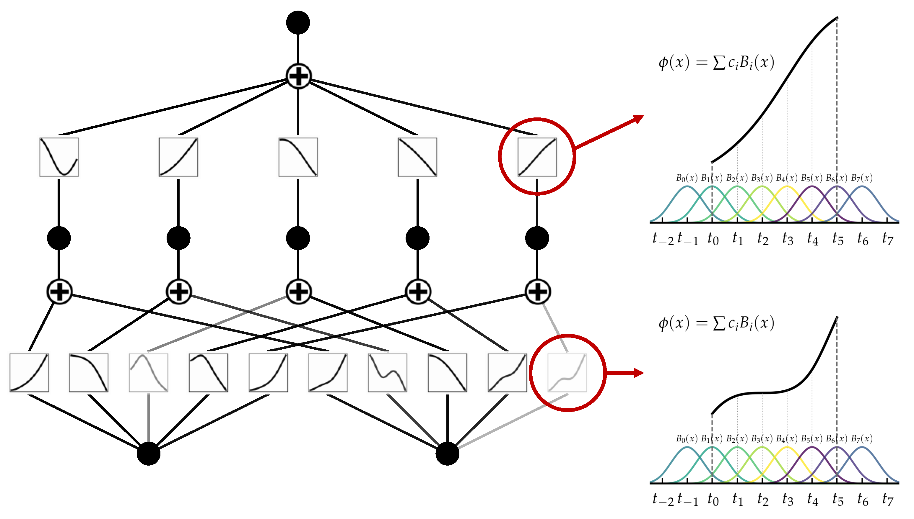
KAN is presented as a potential alternative to the widely used Multi-Layer Perceptrons (MLPs), which are a key component in many deep learning applications. While MLPs rely on constant activation functions on “neurons”, like ReLU or sigmoid, KAN uses learnable activation functions on “edges”, parametrized as k-th order B-spline polynomials. Contrarily to MLPs, this approach allows the network to learn smooth, non-linear trends specifically tailored to the dataset, rather than relying on a predefined, hypothetical non-linearity. Specifically, every activation function is implemented as the sum of a basis function (typically the SiLU function) and the learnable spline component:
where and are trainable weights used to control the magnitude of the basis and spline components, respectively. The spline component is in turn obtained from the summation of n B-spline basis functions , as shown in Figure 7.
Figure 7.
Left: example of KAN, with 2 inlet neurons, one hidden layer with 5 addition neurons and 1 output neuron. Right: activation functions parametrized as summation of B-spline basis multiplied by a corresponding coefficient .
KAN models were implemented using the Pykan library [26]. In a first phase, prediction accuracy of different architectures, following the general guidelines in [26,27], is compared via an extensive parametric study over a large range of KAN hyperparameters, monitoring prediction accuracy to gather general insights on the most relevant hyperparameters. Preliminary sensitivity analysis indicated that model performance is primarily driven by the number of edges in the first layer, the B-spline order k, the number of multiplication subnodes, the number of nodes to be multiplied together (mult_arity), and the grid size. Notably, increasing network depth often led to a sharp degradation in both training and test accuracy, accompanied by higher computational costs; consequently, a more efficient single-hidden-layer architecture was selected. To address the distinct physical aspects of the problem, four independent models were trained to predict: (1) blade geometry, (2) the RMS of the Mach number distribution, (3) the outlet flow angle error, and (4) the kinetic energy loss coefficient. Hyperparameter tuning was conducted via Bayesian Optimization using Optuna [28] to minimize the combined training and test losses, corresponding to, respectively, 70% and 30% of the whole database. The resulting optimal configurations are detailed in Table 3. The training phase utilized the Adaptive Moment Estimation (ADAM) optimizer, with learning rates explored in the range . The grid size was fixed at 5 to balance resolution against the risk of parameter explosion. Finally, performance monitoring on validation sets indicated that optimal convergence was consistently achieved after approximately 200 iterations.
Table 3.
Hyperparameters of the optimized KAN models.
3.2. Model Comparison
To evaluate the most effective modeling strategy, the proposed method was benchmarked against Gaussian Process Regression (GPR) [29] and Multi-Layer Perceptrons (MLPs) [30,31]. Gaussian interpolation approximates a function f using a model , defined as a linear combination of non-linear kernel functions [Equation (10)]:
The Matérn kernel was retained after comparison with alternative kernel functions (RBF, ExpSineSquared, RationalQuadratic), as it provided the lowest mean squared error between predictions and reference data. Once selected, its main hyperparameters, namely the characteristic length () and the smoothness parameter (), were optimized using Optuna. The chosen kernel formulations and their optimized parameters are detailed in Table 4. A constant, shared length scale was applied to all inputs. Except for the RMS target, the resulting optimized kernels exhibit large characteristic lengths. This mathematically signifies a smooth response surface, meaning the predicted outputs do not change rapidly in response to input variations.
Table 4.
Hyperparameters of the optimized GPR models.
As a second baseline, a Multi-Layer Perceptron is considered. An MLP composes affine transformations with non-linear activation functions:
where are trainable parameters and denotes a non-linear activation. The network is trained to minimize the mean squared error (MSE) between predictions and references. Training is performed with the ADAM algorithm. Hyperparameters (depth D, hidden layers width, activation functions and learning rate) are optimized using Optuna to minimize MSE and shown in Table 5. It is important to note that, for all modeling approaches (GPR, MLP, and KAN), an independent model is developed for each target quantity, namely, the geometry, outlet flow angle deviation (), Mach number distribution root mean square error (RMSE), and kinetic energy loss coefficient ().
Table 5.
Hyperparameters of the optimized MLP models.
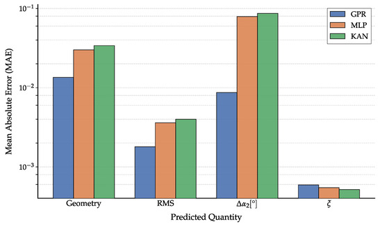
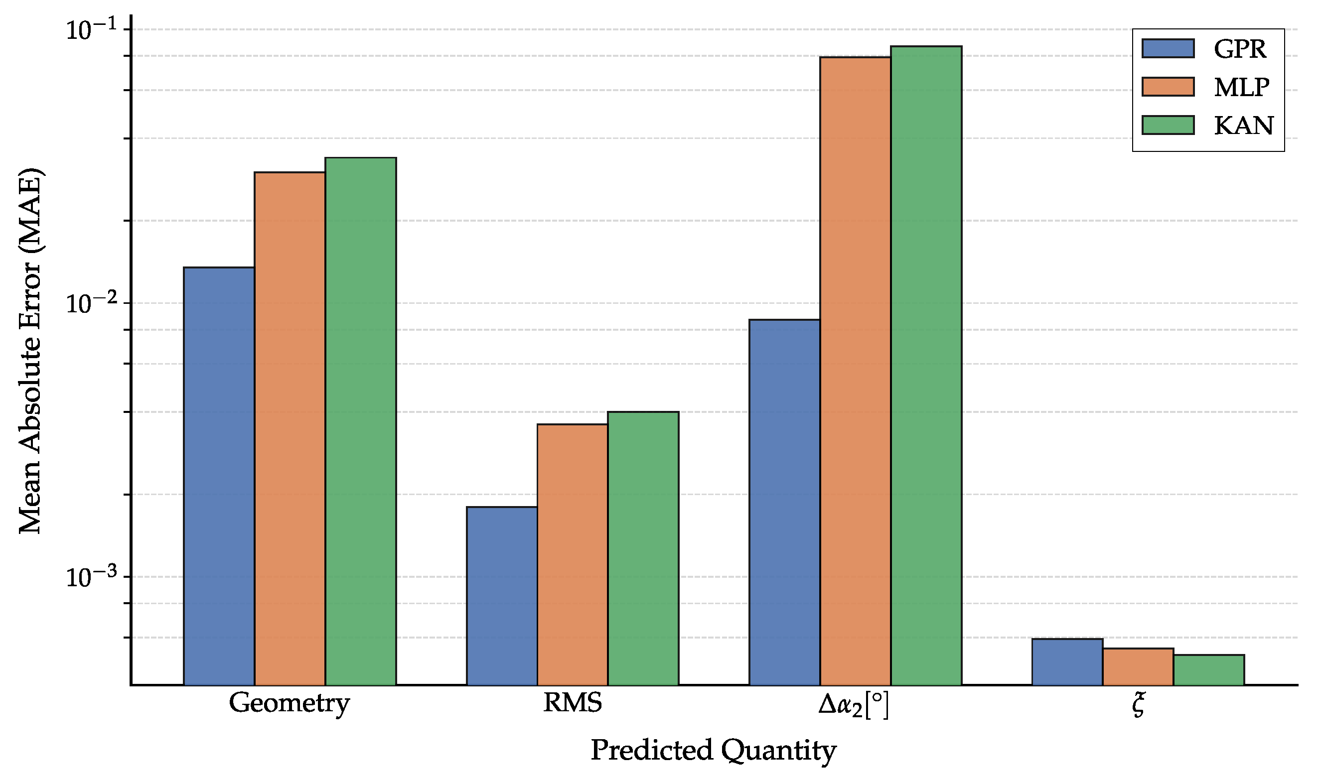
Figure 8 presents a systematic Mean Absolute Error (MAE) comparison across strategies. While GPR achieves the lowest MAE for geometry, RMSE, and , KAN and MLP demonstrate slightly superior robustness for the loss coefficient . However, computational efficiency proves the deciding factor. KAN and MLP offer prediction times of s, whereas GPR averages 120 s due to kernel matrix operations.
Figure 8.
Mean Absolute Error (MAE) on the predictions for the three surrogate models (GPR, MLP, and KAN) across the four predicted quantities: geometry, Mach number RMS, outlet angle deviation (), and kinetic energy loss coefficient ().
For the final models trained with the selected hyperparameters on the same computational platform, KAN and MLP training required only a few minutes, typically of the order of 100–300 s depending on the predicted quantity. In contrast, the exact GPR implementation required several hours for the same dataset size. This limitation is primarily driven by the unfavorable scaling of standard GPR with the number of training samples, due to the repeated kernel-matrix factorization and inversion required during hyperparameter optimization, and is further compounded by the mathematical overhead associated with maximizing the log-marginal likelihood rather than directly minimizing an empirical loss function. In summary, Kolmogorov–Arnold Networks (KANs) deliver the scalability and real-time computational performance required for this study by bypassing the inherent bottlenecks of Gaussian Process Regression. Furthermore, KANs demonstrate superior parameter efficiency, matching the performance of standard Multi-Layer Perceptrons (MLPs) while utilizing significantly fewer parameters.
3.3. Data Selection for Model Training
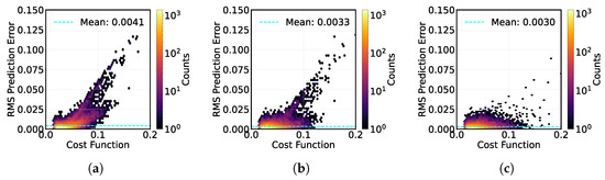
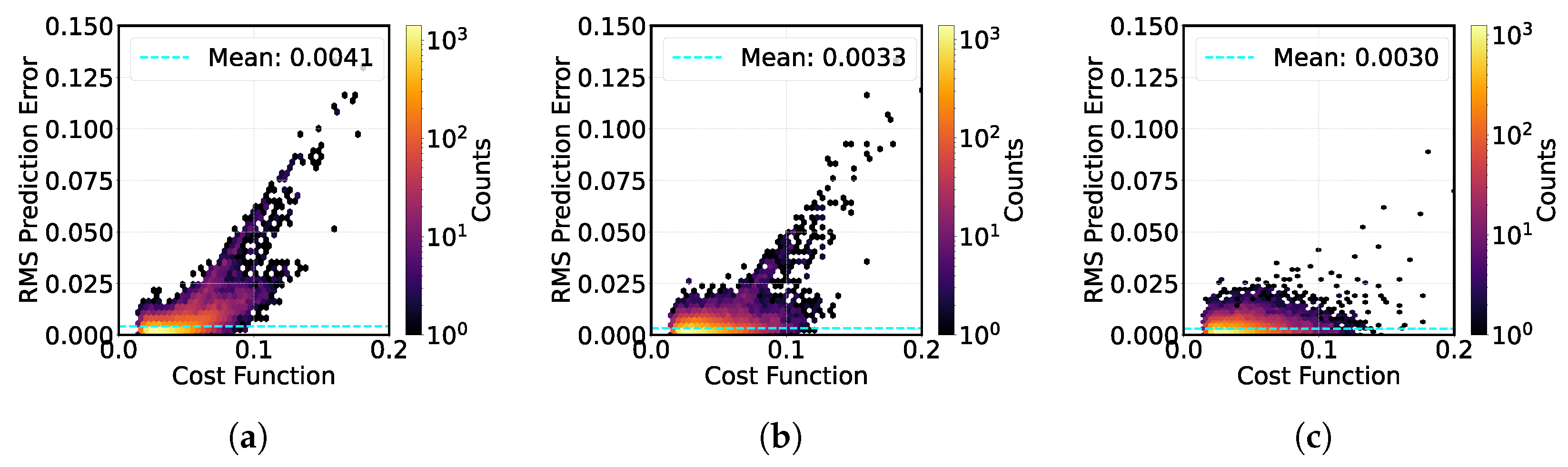
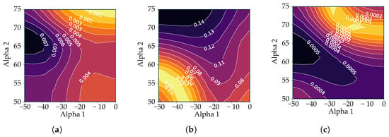
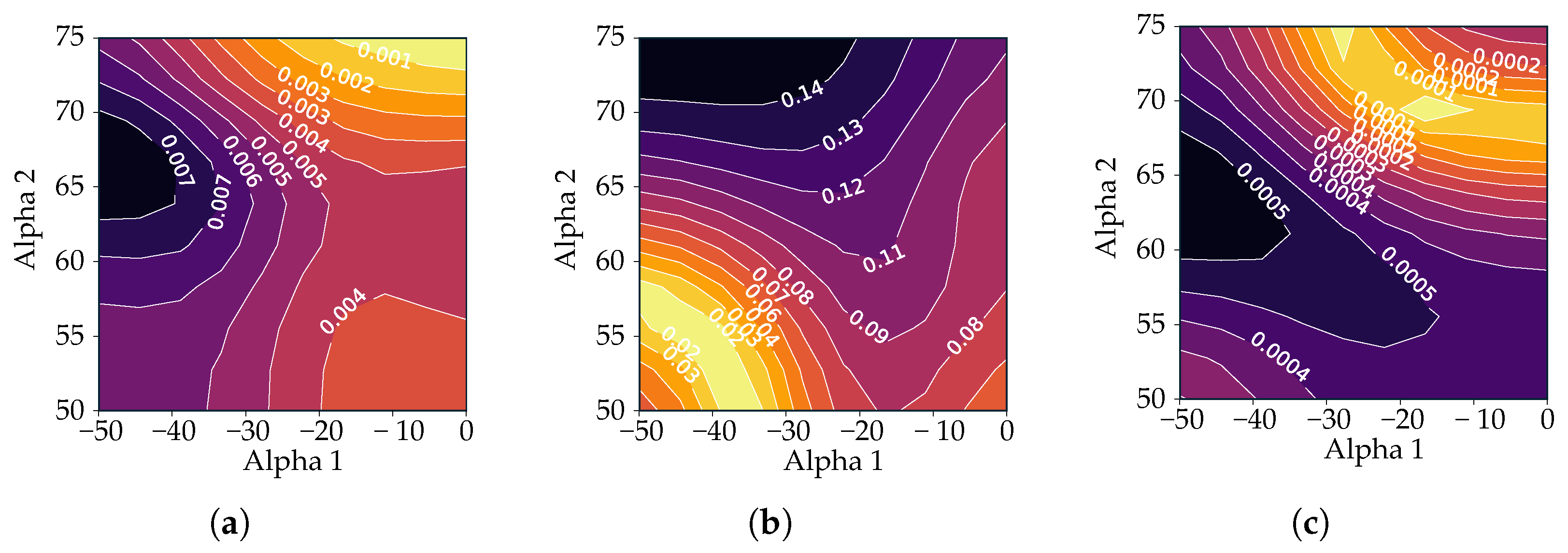
A critical decision in model training is the selection of the dataset. While acceptable convergence is typically defined by an RMSE of 0.03–0.05, certain complex design points exceed this threshold, terminating only due to iteration limits. The inclusion of these high-error samples presents a trade-off: they may enhance generalization by representing difficult regions of the design space or degrade performance by introducing noise. This section investigates the impact of filtering strategies on model accuracy. Guided by the performance analysis in Section 4, we specifically evaluate models trained on database subsets defined by RMSE thresholds of 0.05 and 0.07, representing 71.86% and 89.37% of the total database, respectively. These are benchmarked against an unfiltered model trained on the entire dataset. For simplicity, each model was trained with the same set of hyperparameters mentioned in Table 3. The first analysis focuses on the model designed to predict the RMS error itself. Figure 9 compares three distinct models: (a) trained exclusively on data points with an RMS below 0.05, (b) trained on points with an RMS below 0.07, and (c) trained on the entire database. Although the training sets differ, the predictive capability of each model is evaluated against the complete dataset. Each plot correlates the cost function (Equation (6)) of every database point with its corresponding RMS prediction error, defined as the discrepancy between the model’s predictions and the MISES solver results. In this context, an elevated cost function value signifies reduced physical feasibility for a given design point, whereas a high RMS error denotes a larger deviation between the model’s prediction and the underlying MISES simulations.
Figure 9.
Comparison of predictive performance for the RMS error model across the full database test set. The plots show prediction error versus the cost function value for three distinct training scenarios: (a) model trained only on data with RMSE < 0.05; (b) model trained on data with RMSE < 0.07; and (c) model trained on the complete, unfiltered database.
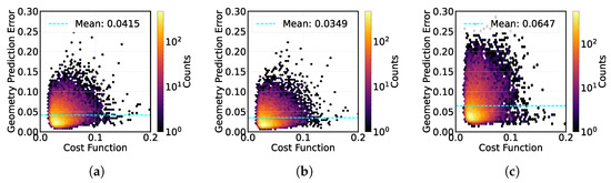
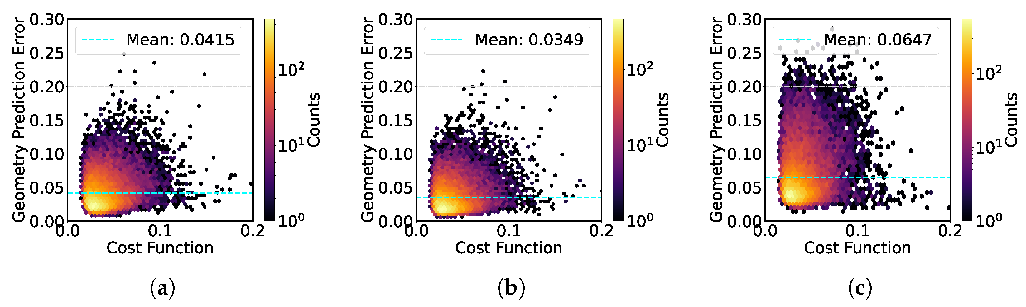
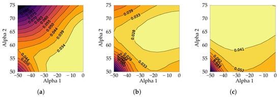
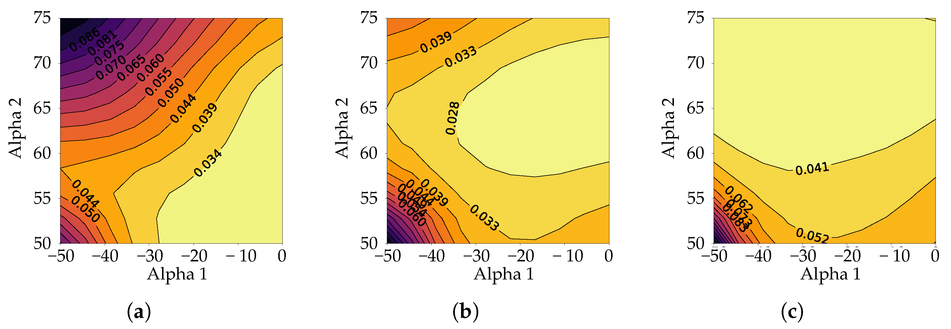
The image demonstrates that, by progressively including points with higher RMS errors (moving from a to c), the model’s overall prediction capability improves. Specifically, the average prediction error decreases from 0.0041 in the most restricted case (a) to 0.0030 in the model trained on the full database (c). This improvement is primarily driven by a significant reduction in prediction error for high-cost function points (the “unfeasible” region on the right side of the plots). By leveraging these challenging, high-RMS design points during the training process, the model is able to develop a more precise understanding of their characteristics. However, this comes with a trade-off: the inclusion of “noisier” data slightly degrades precision in the low-cost region (high-quality points), where the density of low-error predictions is marginally more dispersed in (c) compared to (a). In contrast to the RMS prediction model, the models targeting blade geometry, exit angle error, and kinetic energy loss coefficient exhibit a more complex, non-monotonic response to the composition of the training set. For the sake of brevity, the following analysis focuses on the blade geometry model. However, it is important to note that these findings are representative of the trends observed for both the exit angle error and kinetic energy loss coefficient. As demonstrated in Figure 10 (concerning geometry prediction), it can be seen that the optimal performance is not attained by merely maximizing the dataset size. Conversely, the model that was trained with an intermediate threshold of 0.07 exhibited superior predictive capability in comparison to both the restricted model (threshold 0.05) and the baseline model that was trained on the full database. This identifies a critical trade-off: the 0.05 threshold provides insufficient data for generalization (underfitting), while the full database introduces unfeasible design points acting as noise, which degrades the learning of valid aerodynamic correlations. Rather than strictly defining 0.07 as the absolute optimal balance, as other intermediate values (e.g., 0.06 or 0.08) were not explicitly tested, this result serves to demonstrate a clear non-monotonic trend in model performance. It highlights that an intermediate compromise between data quantity and physical fidelity is necessary to maximize predictive accuracy.
Figure 10.
Comparison of predictive performance for the blade geometry model across the full database test set. The plots show prediction error versus the cost function value for three distinct training scenarios: (a) model trained only on data with RMSE < 0.05; (b) model trained on data with RMSE < 0.07; and (c) model trained on the complete, unfiltered database.
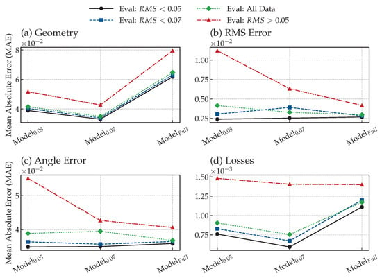
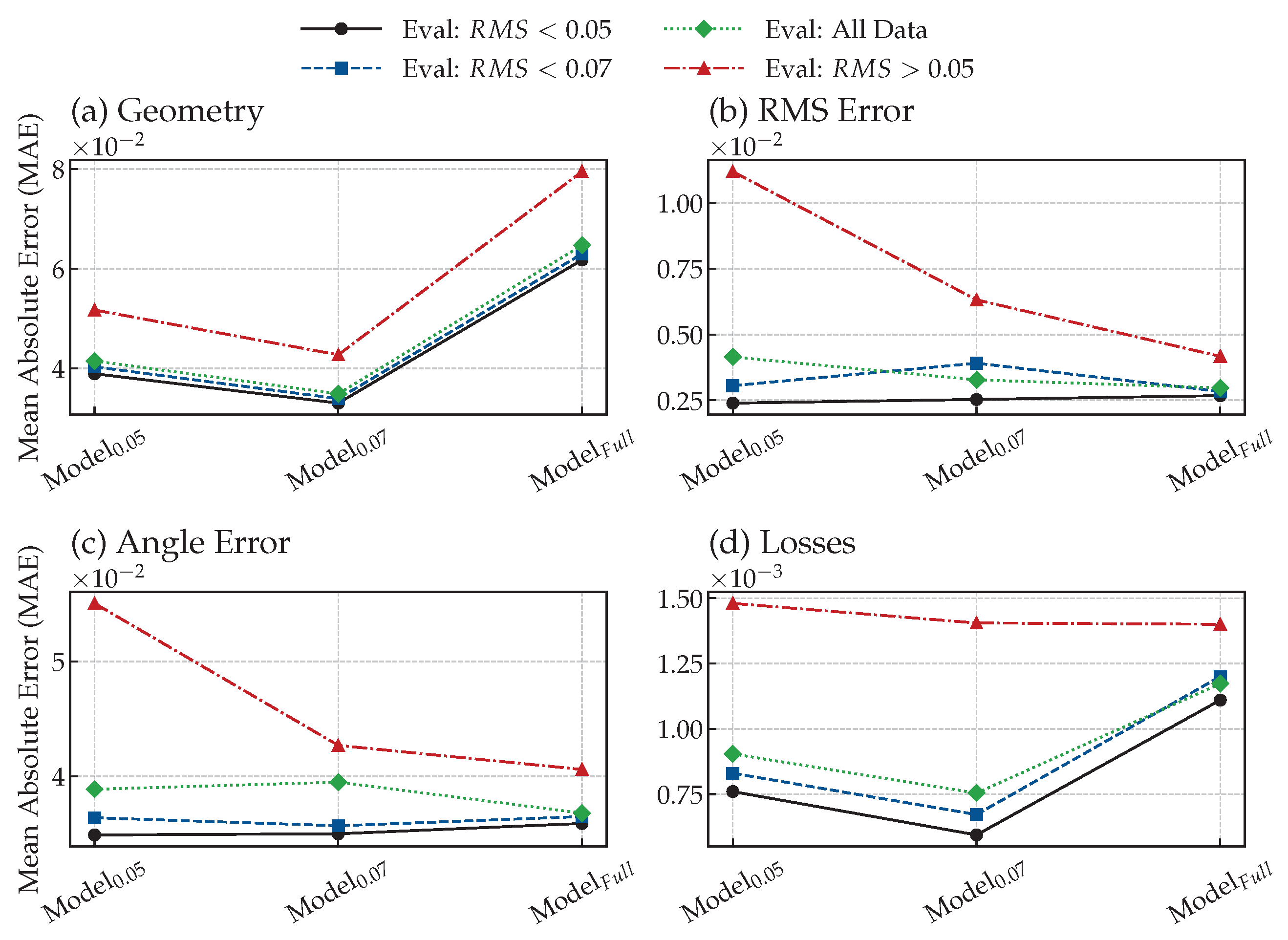
Figure 11 presents a comprehensive analysis of the generalization capabilities of three KAN models across various regions of aerodynamic feasibility. Each model was trained on a distinct subset of the database, categorized by specific RMS error thresholds: 0.05, 0.07, and the unfiltered dataset. The models were subsequently evaluated against four distinct data partitions: a high-accuracy region (RMS < 0.05), a low-accuracy region (RMS > 0.05), an intermediate region (RMS < 0.07), and the complete database. The results demonstrate a non-monotonic trend in predicting both geometry and aerodynamic losses across the full dataset, with achieving the minimum prediction error. Conversely, the model trained on the unfiltered dataset provided the most accurate predictions for flow angle error and overall RMS. Notably, the inclusion of lower-accuracy data during the training phase consistently degraded the models’ predictive performance on the high-accuracy subset (RMS < 0.05). On the other hand, incorporating the full dataset generally enhances the model’s performance when evaluated against the low-accuracy subset (RMS > 0.05). The single notable exception to this broader trend is the prediction of the blade geometry.
Figure 11.
Mean Absolute Error (MAE) of the KAN models evaluated across different data subsets. The performance is assessed for four target metrics: (a) Geometry, (b) RMS Error, (c) Angle Error, and (d) aerodynamic Losses. The plotted lines compare the predictive accuracy of models trained on various datasets ( and ) against a model trained on the full database ().
4. Results and Discussion
The performance of the KAN-based AI tool in terms of computational speed and prediction capability is evaluated in the following section. Moreover, a deep insight into the error classification and design feasibility regions is presented. The model’s evaluation is almost instantaneous. The average blade section design time is ∼0.1 s, denoting a substantial time saving considering the average time of ∼ s required for a singular inverse design during the prior knowledge generation phase. The average outlet flow angle prediction error is , while regarding the Mach number distributions, the RMS error is 0.004. In terms of kinetic energy loss prediction capability, the mean prediction error is 1.46%. In general, an adequately trained KAN regression algorithm demonstrates a considerably high degree of accuracy, thereby facilitating an unbounded and instantaneous exploration of the design space.
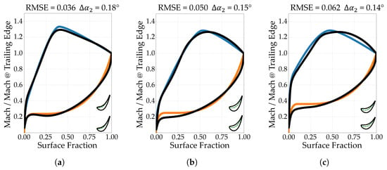
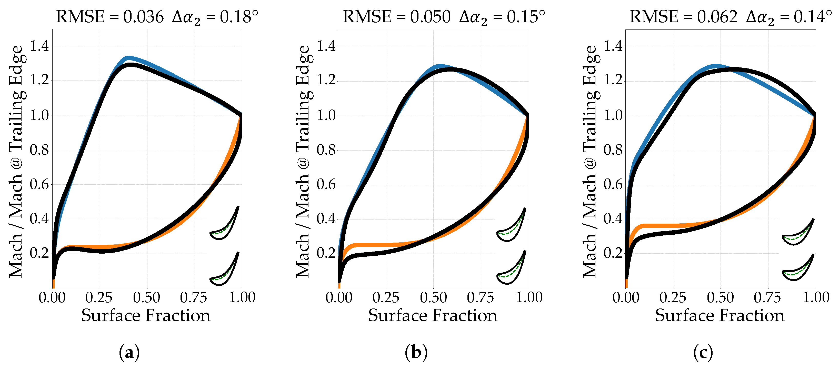
Certain combinations of aerodynamic style (target blade loading distributions) and duty (main flow angles, Mach number and Reynolds) parameters prove unfeasible, causing a discrepancy between the target and actual load distributions that results in high RMSE values. An RMSE of 0.05 is established as the acceptance threshold for the aerodynamic loading, as load variations exceeding this magnitude are widely considered non-negligible in turbomachinery applications. This physical limit is further corroborated by the qualitative assessment in Figure 12. A comparison between the KAN-predicted quantities and the results from MISES simulations confirms the overall reliability of the model across the majority of the design space. As illustrated by the error contours in Figure 13, the model maintains a consistently low prediction error globally. However, a slight degradation in performance is observed at the extremes of the design space, particularly in boundary regions characterized by maximum flow deviation.
Figure 12.
Example of model-generated blades with different and and different target isentropic Mach number distribution on the pressure side (orange) and suction side (magenta), along with the corresponding real load distribution (in black).
Figure 13.
KAN-model prediction error against MISES results for different inlet () and outlet () flow angles of RMS (a), (b) and losses (c).
4.1. Inverse Design Feasibility Space
The model outputs a predicted RMSE value for a specific set of aerodynamic inputs, effectively estimating the discrepancy between the target loading distribution and the resultant real loading distribution. High RMS error regions identify non-viable parameter combinations in the design space. Figure 14 shows the distribution of the predicted RMS error with respect to the inlet flow angle () and the outlet flow angle () for different peak Mach number axial positions (), with a fixed relative value of 1.25. The darker colors represent regions of the design space characterized by a high RMS, corresponding to zones where a viable design is not possible. Conversely, the lighter colors represent recommended design zones.
Figure 14.
Root mean square error prediction for different inlet () and outlet () flow angles. The figures show the trend going from loaded blades with equal to 0.3 (a), 0.5 (b) and 0.7 (c) with a fixed value of equal to 1.25 and and equal to 0.85 and 1.4, respectively.
This analysis establishes the existence of any correlation between variations in flow angles, with a fixed peak Mach number amplitude, and the shift in the throat position along the surface fraction for optimal turbine designs. In contrast, the viable design space for front-loaded blades (Figure 14a) is constrained, primarily limited to low absolute values () and moderately low . These unfeasible combinations of aerodynamic duty parameters highlight intrinsic geometrical constraints. As approaches zero, the stagger angle tends to increase, which naturally shifts the throat region towards the leading edge, resulting in front-loaded profiles. On the contrary, shifting the throat region toward the trailing edge (aft-loaded configurations) renders the near-zero design space progressively unfeasible. Figure 15 denotes an extreme point of the design space, along with the corresponding blade geometry and Mach number distribution for the front-loaded scenario ().
Figure 15.
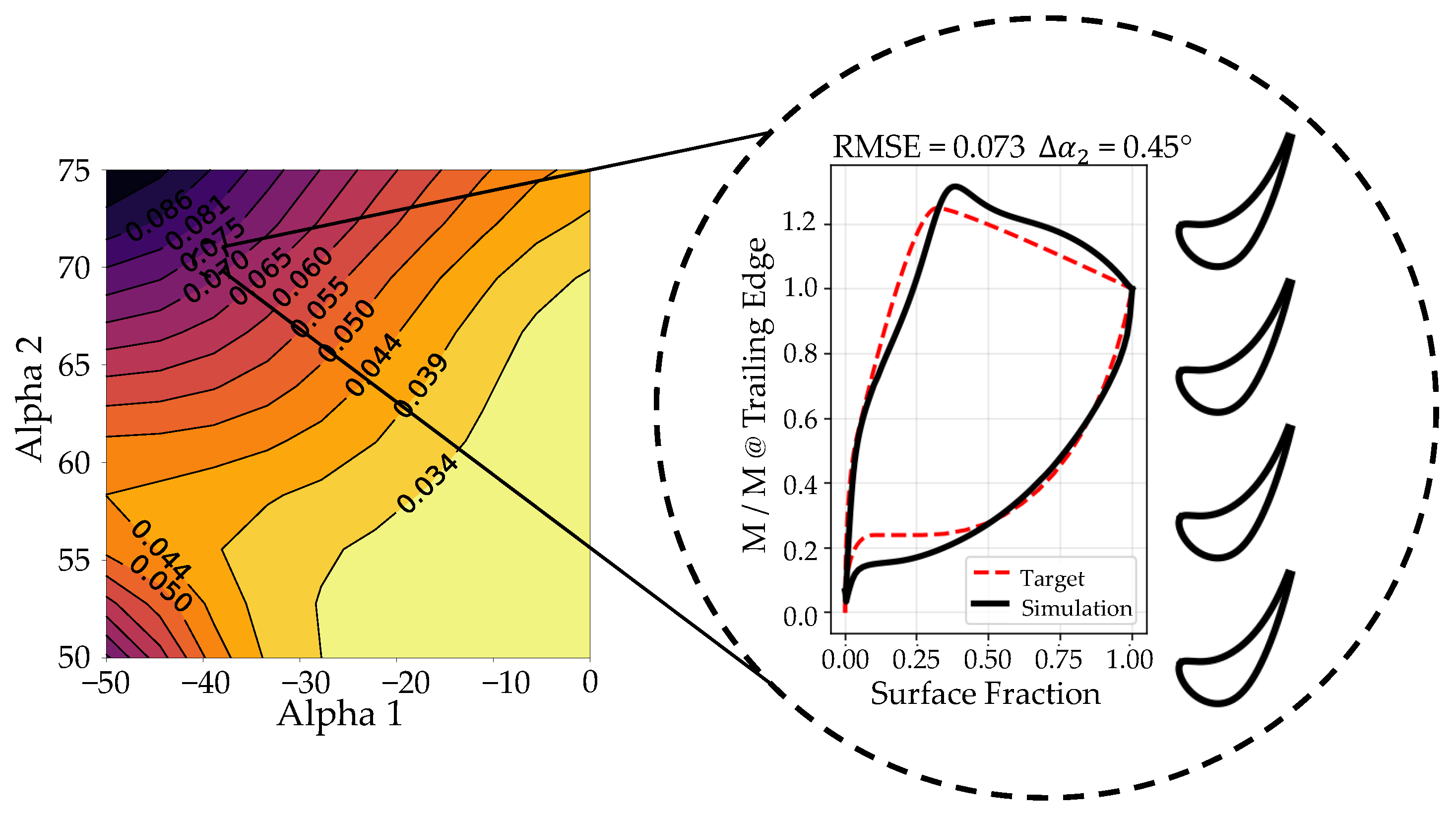
Left: The model’s predicted root mean square error for different inlet () and outlet () flow angles for aft-loaded blades ( equal to 0.7). Right: An extreme point of the design space is highlighted, characterized by equal to and equal to , with the corresponding blade geometry and real vs. target loading distribution.
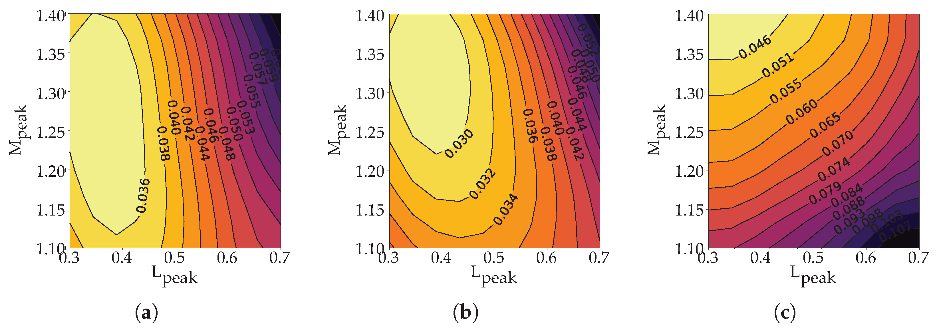
A second study is dedicated to analyzing the coupled influence of the peak Mach number () and its axial position () on the design space (Figure 16), with respect to the target aerodynamic duty.
Figure 16.
Model’s predicted root mean square error for different peak Mach number position () and value (). The figures show the trend going from axial inlet flow with equal to 0 (a), (b) and a more tangential inlet flow with equal to (c). The outlet flow angle is fixed at .
With fixed at , varying reveals a strong dependency between the inlet angle and the feasibility boundary. As increases from to , the feasible region shifts toward higher values and becomes increasingly constrained to values near 0.38, dropping off sharply elsewhere. This confirms that for low outlet angles, increasing the inlet angle enforces a strict requirement for high, upstream acceleration.
4.2. Guidelines for Inverse Blade Design
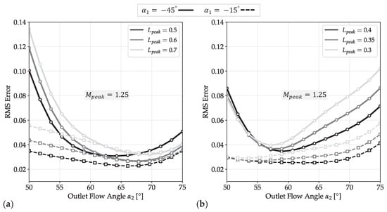
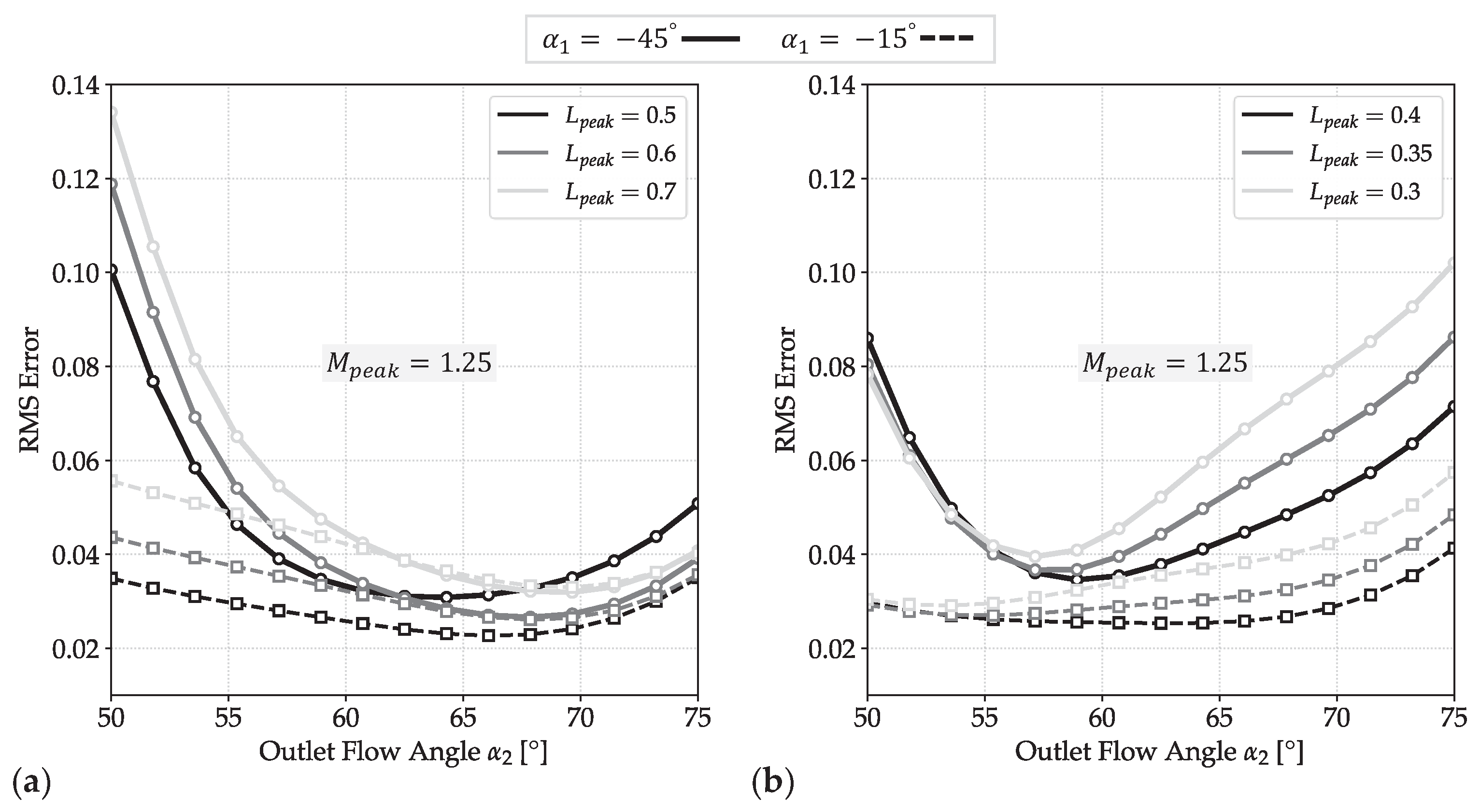
Following an assessment of the prediction accuracy of the design tool, a comprehensive analysis of the design space has enabled the identification of certain design criteria in relation to performance and geometric guidelines. A sensitivity analysis identifies the inlet and outlet flow angles () and the peak Mach number magnitude and position () as the primary drivers of blade design. Since variations in these four parameters induce the most significant geometric changes, the cross-effects of these governing variables are systematically analyzed and summarized in Figure 17 and Figure 18. Figure 17a illustrates that mid-to-aft loaded blades ( between and ) yield a significantly broader feasible design space, exhibiting reduced RMS errors, especially at large outlet flow angles (). This configuration facilitates larger flow turning. Furthermore, as increases, the predicted RMS error consistently diminishes, reaching a distinct minimum in the range of to . This minimum identifies the region of optimal compatibility for the design parameters. Increasing the tangential inlet flow component (higher ) is critical at low values, significantly narrowing the feasible region for nearly symmetric blades. However, at higher flow deviations, this constraint relaxes, and the feasible range recovers to match that of nearly axial flow designs. In contrast, the feasible design space for front-loaded profiles () as shown in Figure 17b is highly restricted, being primarily confined to low absolute inlet flow angles () and moderate outlet flow angles. Increasing the magnitude of renders the design space largely infeasible; the model identifies a narrow stability window for between and , with rapid divergence observed outside this interval. This trend is physically consistent. Front-loaded blades impose strong leading-edge acceleration, requiring high curvature and a relatively large frontal thickness, which increases blockage and local Mach number. For cascades with high inlet angle and high inlet Mach number, this can lead to excessive leading-edge loading and therefore to incompatible target distributions. Conversely, front loading remains feasible for vanes with nearly axial inlet flow, low inlet Mach number, and limited turning.
Figure 17.
Design feasibility represented by RMS error trends plotted against outlet flow angle for various inlet flow angles , comparing (a) aft-loaded and (b) front-loaded blade designs.
Figure 18.
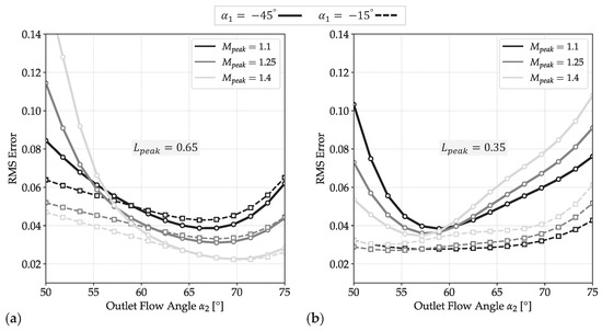
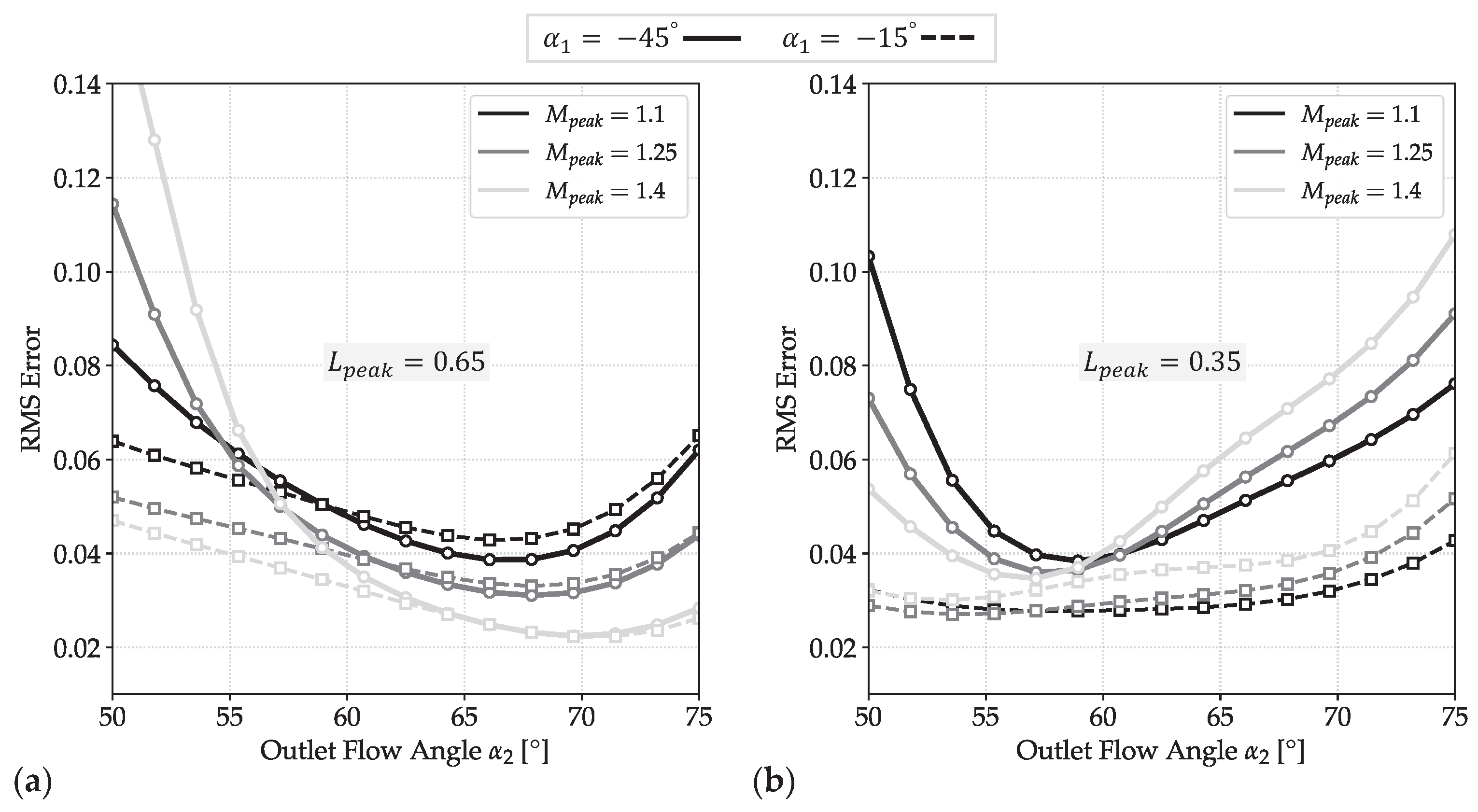
Design feasibility represented by RMS error trends plotted against outlet flow angle for various inlet flow angles and peak Mach number magnitude , comparing (a) aft-loaded and (b) front-loaded blade designs.
Figure 18a,b shows the effect on design feasibility of the peak Mach number amplitude () for both aft-loaded (a) and front-loaded (b) blades. Figure 18a highlights a consistent trend for high outlet flow angles independent of the inlet flow direction, suggesting that designs characterized by higher suction-side velocities exhibit greater feasibility. In the low regime, the inlet flow direction becomes a critical factor for design feasibility: near-axial inflows allow for higher peak Mach numbers (), whereas highly tangential inflows require reduced flow acceleration to guarantee the aerodynamic feasibility. In contrast, front-loaded blades (Figure 18b) exhibit an opposing trend. While the optimal feasibility window remains centered in a range of between and , these designs generally favor restricted peak Mach numbers. An exception occurs at high tangential inlet flows combined with low , where the minimum RMS error shifts towards a maximum of 1.4. For symmetric flow conditions (), the predicted RMS error consistently exceeds the feasibility threshold.
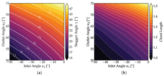
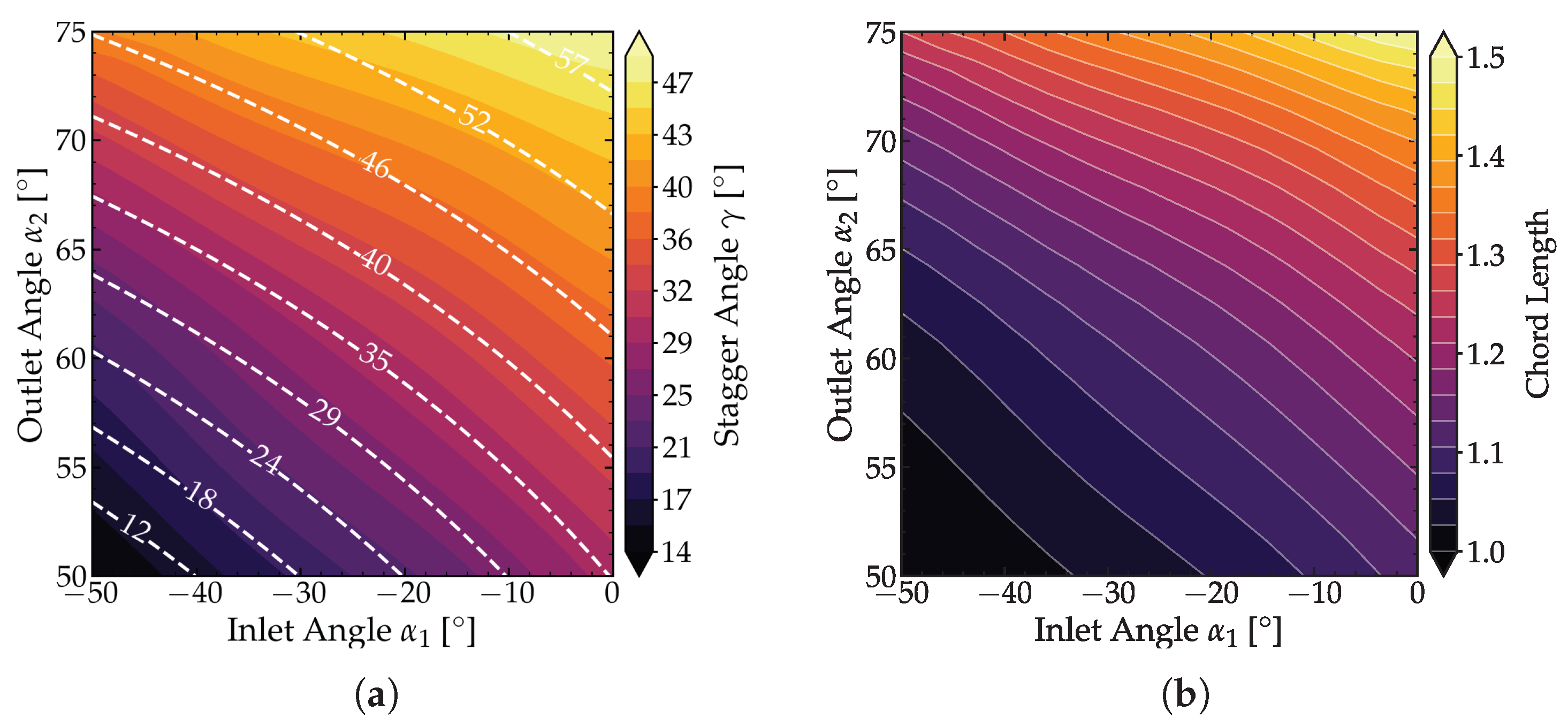
Although symmetric blading is well-established in the literature, its geometric requirements diverge from the generalized aerodynamic correlations captured by the model. This discrepancy indicates that impulse stages require distinct design strategies that deviate from the predominant trends assimilated from the training dataset. Finally, a summary of the key guidelines for the geometric design of blades as a function of the flow angles is provided in Figure 19 and Figure 20. This analysis was conducted under a mean aerodynamic style, with values and or 1.4 and 0.85, respectively, and and of 1.25 and 0.5. The key parameters under analysis are the stagger angle (), blade area, pitch-to-chord ratio, and chord length (C). Both the stagger angle and the chord exhibit the same monotonically increasing trend as the flow progressively aligns with the axial inlet direction (as increases toward ). Furthermore, both increase as the outlet flow angle () increases. Notably, the derived stagger angles show strong agreement with Kacker and Okapuu [24].
Figure 19.
Influence of inlet () and outlet () flow angles on key blade geometric parameters: (a) Stagger Angle and (b) Chord Lenght C. The value of the stagger angle is compared against Kacker & Okapuu’s [24] correlation, represented by the white dashed lines.
Figure 20.
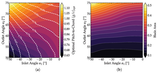
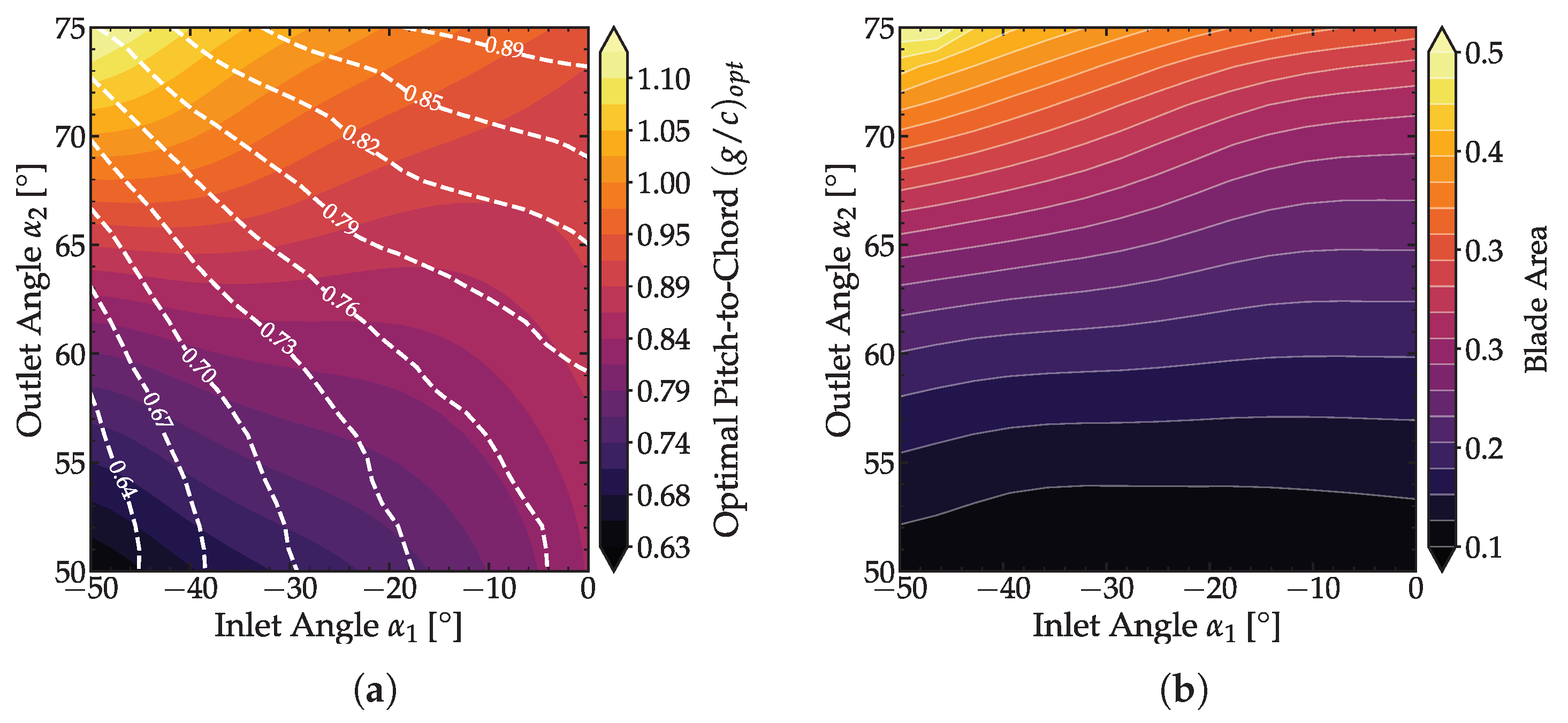
Influence of inlet () and outlet () flow angles on key blade geometric parameters: (a) Pitch-to-chord ratio, and (b) Blade Area. The pitch-to-chord ratio is compared against Dejc & Trojanovskij’s [32] correlation, represented by the white dashed lines.
In contrast, the blade area presents a monotonically decreasing trend, progressively thinning as the inlet flow angle () tends towards , but still increasing as increases. The trend of the pitch-to-chord ratio is strongly influenced by the value of , tending towards an asymptotic value of approximately for every value as tends towards . While demonstrating a qualitatively similar trend to the Dejc and Trojanovsky correlation, quantitative discrepancies arise from diverging objectives. The classical correlation optimizes solidity to minimize profile losses, whereas our framework determines the pitch required to sustain a target aerodynamic loading (, ).
The trends observed for all four quantities (stagger angle , blade area, pitch-to-chord ratio, and blade chord C) remain remarkably consistent across the entire range of flow angles, despite variations in the critical aerodynamic style parameters , , , and . Although the absolute numerical values of and C change proportionally to the changes in these aerodynamic variables, the shape and direction of their relationship with the inlet flow angle are preserved. This indicates the robustness of the fundamental geometric requirements across different operating conditions and aerodynamic constraints.
5. Conclusions
This work presents a data-driven framework for the inverse design of high-Re 2D uncooled turbine blades, employing a Kolmogorov–Arnold Network (KAN) to bypass the computational cost of direct CFD solvers and clearly define feasible loading targets. The model was trained on a high-fidelity database of ≈30,000 profiles, each generated via a MISES-coupled optimization pipeline minimizing target Mach distribution RMSE. In this study, we implemented Kolmogorov–Arnold Networks trained on aerodynamically resolved MISES solver results to address the computational limitations of Gaussian Process Regression. The results demonstrated that this approach ensures the scalability required for real-time applications, accelerating prediction times from for GPR down to . Furthermore, the evaluation showed that a single-layer KAN architecture achieves accuracy and efficiency comparable to traditional MLPs that require four to five layers and hundreds of neurons, maintaining a markedly more efficient parameter footprint. Crucially, a systematic data selection study demonstrated that maximizing dataset size does not universally improve model accuracy. While the full database aids in mapping unfeasible regions, the inclusion of high-RMS error results acts as noise when predicting physical parameters (geometry, losses, angle or RMSE). An intermediate filtering threshold () was identified for geometry prediction and aerodynamic losses as the optimal compromise between data volume and physical fidelity, outperforming both the unfiltered database and strictly restricted subsets. A key contribution is the derivation of a quantitative feasibility metric from the model’s RMS error prediction, enabling the generation of maps that rigorously delineate the inverse design space. Sensitivity analysis identified flow angles () and peak loading parameters () as the primary topological drivers, revealing distinct aerodynamic trade-offs. Aft-loaded designs () exhibited the broadest feasibility, particularly at , favoring higher under high turning but requiring reduced acceleration at tangential inflows. In contrast, front-loaded profiles (–0.4) proved significantly more constrained, limited to a narrow stability window () and generally lower peak velocities, except for specific high-inlet-turning/low-outlet-angle regimes where viability shifted toward maximal (). Finally, robust correlations between geometric features (stagger, chord, pitch) and flow angles were established across diverse loading styles, providing validated initialization points for future campaigns. Ultimately, this tool accelerates the design cycle by four orders of magnitude, offering immediate, physics-based feedback on conceptual viability.
Author Contributions
Conceptualization, F.P., A.P. and S.L.; methodology, F.P., A.P. and S.L.; software, F.P.; validation, F.P.; formal analysis, F.P.; investigation, F.P.; resources, S.L.; data curation, F.P.; writing—original draft preparation, F.P.; writing—review and editing, S.L.; visualization, F.P.; supervision, S.L.; project administration, S.L.; funding acquisition, S.L. All authors have read and agreed to the published version of the manuscript.
Funding
The authors state that no funds or other financial support were received during the preparation of the article.
Data Availability Statement
The data that support the findings of this study are available from the corresponding author upon reasonable request.
Acknowledgments
The authors acknowledge the speech given by C. Clark at the Spleen workshop, which served as a cornerstone for this study.
Conflicts of Interest
The authors declare no conflicts of interest.
Abbreviations
The following abbreviations are used in this manuscript:
| ADAM | Adaptive Moment Estimation |
| AI | Artificial Intelligence |
| ANN | Artificial Neural Networks |
| AVDR | Axial Velocity Density Ratio |
| CFD | Computational Fluid Dynamics |
| CPU | Central Processing Unit |
| DNS | Direct Numerical Simulation |
| DOF | Degree Of Freedom |
| GPR | Gaussian Process Regression |
| KAN | Kolmogorov–Arnold Networks |
| LES | Large Eddy Simulation |
| LHS | Latin Hypercube Sampling |
| MAE | Mean Absolute Error |
| MISES | Multiple blades Interacting Streamtube Euler Solver |
| ML | Machine Learning |
| MLPs | Multi-Layer Perceptrons |
| MOGP | Multi-Output Gaussian Process |
| MSE | Mean Square Error |
| Probability Density Function | |
| POD | Proper Orthogonal Decomposition |
| PS | Pressure Side |
| RANS | Reynolds-Averaged Navier–Stokes |
| RMS | Root Mean Square |
| RMSE | Root Mean Square Error |
| SS | Suction Side |
| Nomenclature | |
| Bernstein polynomial coefficients | |
| B-spline basis | |
| b | Bias |
| C | Blade chord |
| Axial chord | |
| Class function | |
| L | Curvilinear abscissa |
| Axial position of peak Mach number | |
| M | Mach number |
| Magnitude of the peak Mach number | |
| P | Pressure |
| Control points | |
| Reynolds number | |
| R | Radius |
| S | Shape function |
| Maximum camber line curvature point X coordinate | |
| Maximum camber line curvature point Y coordinate | |
| Greek Symbols | |
| Inlet Flow angle | |
| Outlet Flow angle | |
| Annealing coefficient | |
| Stagger angle/Specific heat ratio | |
| Thickness distribution | |
| Kernel function | |
| Mean value | |
| Matern kernel shape parameter | |
| Kinetic energy loss coefficient | |
| Standard deviation | |
| Activation function | |
| Inlet metal angle | |
| Outlet metal angle | |
| Normalized chord coordinate | |
| Subscripts | |
| 0 | Total/stagnation quantity |
| 1 | Inlet section |
| 2 | Outlet section |
| Axial component | |
| Camber line | |
| Isentropic | |
| Leading Edge | |
| Peak Mach number | |
| Pressure Side | |
| Suction Side | |
| Trailing Edge | |
References
- Pierret, S.; Van den Braembussche, R.A. Turbomachinery blade design using a Navier-Stokes solver and artificial neural network. J. Turbomach. 1999, 121, 326–332. [Google Scholar] [CrossRef] [Scilit]
- Kosowski, K.; Tucki, K.; Kosowski, A. Turbine stage design aided by artificial intelligence methods. Expert Syst. Appl. 2009, 36, 11536–11542. [Google Scholar] [CrossRef] [Scilit]
- Du, Q.; Li, Y.; Yang, L.; Liu, T.; Zhang, D.; Xie, Y. Performance prediction and design optimization of turbine blade profile with deep learning method. Energy 2022, 254, 124351. [Google Scholar] [CrossRef] [Scilit]
- Zhang, C.; Janeway, M. Optimization of turbine blade aerodynamic designs using CFD and neural network models. Int. J. Turbomach. Propuls. Power 2022, 7, 20. [Google Scholar] [CrossRef] [Scilit]
- Li, Z.; Liu, Y.; Yang, J.G.; Wang, H.Q. A data-based policy model for intelligent turbine cascade design. J. Appl. Fluid Mech. 2022, 15, 1179–1192. [Google Scholar] [CrossRef] [Scilit]
- Li, J.; Zhang, M.; Martins, J.R.; Shu, C. Efficient aerodynamic shape optimization with deep-learning-based geometric filtering. AIAA J. 2020, 58, 4243–4259. [Google Scholar] [CrossRef] [Scilit]
- Li, J.; Zhang, M. Data-based approach for wing shape design optimization. Aerosp. Sci. Technol. 2021, 112, 106639. [Google Scholar] [CrossRef] [Scilit]
- Maral, H.; Alpman, E.; Kavurmacıoğlu, L.; Camci, C. A genetic algorithm based aerothermal optimization of tip carving for an axial turbine blade. Int. J. Heat Mass Transf. 2019, 143, 118419. [Google Scholar] [CrossRef] [Scilit]
- Angelini, G.; Corsini, A.; Lavagnoli, S. Machine-learnt topology of complex tip geometries in gas turbine rotors. Proc. Inst. Mech. Eng. Part A J. Power Energy 2020, 235, 383–392. [Google Scholar] [CrossRef] [Scilit]
- Li, J.; Wang, Y.; Qiu, Z.; Zhang, D.; Xie, Y. Fast performance prediction and field reconstruction of gas turbine using supervised graph learning approaches. Aerosp. Sci. Technol. 2023, 140, 108425. [Google Scholar] [CrossRef] [Scilit]
- Senior, A.; Miller, R. A data-centric approach to loss mechanisms. J. Turbomach. 2023, 146, 011006. [Google Scholar] [CrossRef] [Scilit]
- Clark, C.J. A step towards an intelligent aerodynamic design process. In ASME Turbo Expo 2019: Turbomachinery Technical Conference and Exposition; (GT2019-90204); American Society of Mechanical Engineers: New York, NY, USA, 2019. [Google Scholar] [CrossRef] [Scilit]
- Bellucci, J.; Granata, A.A.; Silei, M.; Giovannini, M.; Spano, E.; Notaristefano, A.; Lengani, D. A real-time AI-based strategy for the design of a low-pressure turbine profile. In ASME Turbo Expo 2024: Turbomachinery Technical Conference and Exposition; (GT2024-128809); American Society of Mechanical Engineers: New York, NY, USA, 2024. [Google Scholar] [CrossRef] [Scilit]
- Petronio, D.; Paliotta, P.; Lengani, D.; Simoni, D. A ML strategy for the identification of optimal LPT design region and related blade shape. Aerosp. Sci. Technol. 2024, 148, 109118. [Google Scholar] [CrossRef] [Scilit]
- Zou, Z.; Xu, P.; Chen, Y.; Yao, L.; Fu, C. Application of artificial intelligence in turbomachinery aerodynamics: Progresses and challenges. Artif. Intell. Rev. 2024, 57, 222. [Google Scholar] [CrossRef] [Scilit]
- Coull, J.D. Endwall Loss in Turbine Cascades. J. Turbomach. 2017, 139, 081004. [Google Scholar] [CrossRef] [Scilit]
- Kulfan, B.M. Universal parametric geometry representation method. J. Aircr. 2008, 45, 142–158. [Google Scholar] [CrossRef] [Scilit]
- Kulfan, B.M. Recent extensions and applications of the CST universal parametric geometry representation method. Aeronaut. J. 2010, 114, 157–176. [Google Scholar] [CrossRef] [Scilit]
- Kulfan, B.; Bussoletti, J. Fundamental parametric geometry representations for aircraft component shapes. In Proceedings of the 11th AIAA/ISSMO Multidisciplinary Analysis and Optimization Conference, Portsmouth, VA, USA, 6–8 September 2006; p. 6948. [Google Scholar] [CrossRef] [Scilit]
- Drela, M.; Youngren, H. A User’s Guide to MISES 2.53; MIT Computational Aerospace Sciences Laboratory: Cambridge, MA, USA, 1998; Available online: https://web.mit.edu/drela/Public/web/mises/mises.pdf (accessed on 1 January 2024).
- Delvaux, G.; Toracchio, R.; Boufidi, E.; Croner, E.; Fontaneto, F. The Modeling of Roughness Effect on the Performance of a Controlled Diffusion Airfoil. ASME. J. Turbomach. 2022, 145, 021008. [Google Scholar] [CrossRef] [Scilit]
- Andrew, P.L.; Kahveci, H.S. Validation of MISES Two-Dimensional Boundary Layer Code for High-Pressure Turbine Aerodynamic Design. ASME. J. Turbomach. 2009, 131, 031013. [Google Scholar] [CrossRef] [Scilit]
- Nelder, J.A.; Mead, R. A simplex method for function minimization. Comput. J. 1965, 7, 308–313. [Google Scholar] [CrossRef] [Scilit]
- Kacker, S.C.; Okapuu, U. A mean line prediction method for axial flow turbine efficiency. ASME J. Eng. Power 1982, 104, 111–119. [Google Scholar] [CrossRef] [Scilit]
- Brown, L.E. Axial flow compressor and turbine loss coefficients: A comparison of several parameters. J. Eng. Power 1972, 94, 193–201. [Google Scholar] [CrossRef] [Scilit]
- Liu, Z.; Wang, Y.; Vaidya, S.; Ruehle, F.; Halverson, J.; Soljacic, M.; Hou, T.Y.; Tegmark, M. KAN: Kolmogorov–Arnold networks. arXiv 2024. [Google Scholar] [CrossRef] [Scilit]
- Liu, Z.; Ma, P.; Wang, Y.; Matusik, W.; Tegmark, M. KAN 2.0: Kolmogorov–Arnold networks meet science. arXiv 2024. [Google Scholar] [CrossRef] [Scilit]
- Akiba, T.; Sano, S.; Yanase, T.; Ohta, T.; Koyama, M. Optuna: A next-generation hyperparameter optimization framework. In Proceedings of the 25th ACM SIGKDD International Conference on Knowledge Discovery & Data Mining, Anchorage, AK, USA, 4–8 August 2019; pp. 2623–2631. [Google Scholar] [CrossRef] [Scilit]
- Géron, A. Hands-on Machine Learning with Scikit-Learn, Keras, and TensorFlow: Concepts, Tools, and Techniques to Build Intelligent Systems, 2nd ed.; O’Reilly Media: Santa Rosa, CA, USA, 2019. [Google Scholar]
- Rumelhart, D.E.; Hinton, G.E.; Williams, R.J. Learning representations by back-propagating errors. Nature 1986, 323, 533–536. [Google Scholar] [CrossRef] [Scilit]
- Goodfellow, I.; Bengio, Y.; Courville, A. Deep Learning; MIT Press: Cambridge, MA, USA, 2016; Available online: http://www.deeplearningbook.org (accessed on 1 February 2025).
- Dejc, M.E.; Trojanovskij, B.M. Unterssuchung und Berechung Axialer Turbinenstufen; VEB Verlag Technik: Berlin, Germany, 1973. [Google Scholar]

Disclaimer/Publisher’s Note: The statements, opinions and data contained in all publications are solely those of the individual author(s) and contributor(s) and not of MDPI and/or the editor(s). MDPI and/or the editor(s) disclaim responsibility for any injury to people or property resulting from any ideas, methods, instructions or products referred to in the content. |
© 2026 by the authors. Licensee MDPI, Basel, Switzerland. This article is an open access article distributed under the terms and conditions of the Creative Commons Attribution (CC BY) license.