


Abstract
In this study, experimental quantification of drainage potential curves for unspiked and spiked Exxsol D60 was performed and compared against simplified numerical model results. This potential relates to the flow rate of tapped water from the bottom of the pipe to the water cut of the tapped stream. To mimic the separation characteristics of a real crude-water mixture, Exxsol D60 was spiked with small amounts of crude oil. A pipe separator with two parallel branches and one tapping point was used to measure drainage potential experimentally. There was a slight decrease in separation performance for the spiked Exxsol D60 in general when compared with the unspiked oil’s drainage potential curves. However, for low inlet water cuts, the performance of the former was significantly worse than the latter. There was, in general, a fair agreement between experimental and numerical drainage potential curves. The flow patterns of the oil–water mixture approaching the tapping point are the major determining factors of drainage potential curves. Results of this work could be employed to predict the performance and design of bulk oil–water pipe separators that have one or multiple tapping points.
1. Introduction
It is common for water to be produced along with oil and gas during the exploitation of underground reservoirs. Water can come from several sources, e.g., connate water in the pores of the producing reservoir layers, water from aquifer layers flowing into the well, associated water with produced gas, or from water injection for pressure support and oil displacement [1]. If water production is excessive, it often reaches the processing capacity of topside facilities, prohibiting maintaining or increasing oil production. This situation is typically called bottlenecking. Therefore, the handling of produced water is and will continue to be an essential task for the operators. Improving water-oil separation methods and/or bringing more capacity will hopefully help with debottlenecking [2].
Part of the water-oil separation is conducted in a first-stage bulk separator that uses gravity vessels to lower the oil concentration to 500–1000 ppmW [3]. Bulk oil–water separation equipment is typically installed topside of offshore installations. However, subsea deployments have been proposed as a measure to debottleneck topside facilities, enable subsea re-injection, and as they offer some advantages with respect to conventional topside deployments. For example, in a subsea installation, the water-oil mixture travels a shorter distance from the wellhead before separating, therefore the pressure loss in the flow lines is reduced [4,5], and there is less mixing and emulsification. This gives better separation and allows production of higher rates for a longer time.
Another benefit of a subsea installation is the flexibility it provides; bulk liquid–liquid separation units can be added on the subsea without adding weight and occupying the footprint of an offshore topside structure. Subsea units can be deployed if needed throughout the field design and development phase, without the operator having to leave an extra accessible area or weight carrying capacity [6]. Some modern pipe separators have been recently developed and employed to separate produced water, such as Marlim, Saipem’s SpoolSep, and Horizontal Pipe Separator (HPS) [7,8,9].
In this work, we focus on further advancement of experimental procedures and design methods for a bulk pipe oil–water separator for subsea applications. Our research is part of the SUBPRO research center, and it is a continuation of the work by Skjefstad (2019) [10]. Skjefstad (2019) developed a parallel pipe bulk oil–water separator, built a prototype, and conducted several experimental campaigns to quantify its performance, optimize its design, and assess the influence of surfactants and inlet choking, among other factors [2,3,4,5,6,7,8,9,10,11]. The separator is intended to be installed downstream of a gas separation unit, thus it handles oil and water only.
The first gap the current study addresses is the use of crude oil as a surfactant to the oil–water mixture to achieve separation characteristics closer to a real crude-water fluid system. The previous research by Skjefstad (2019) was made using Exxsol D60 and brine. It is often reported in the literature that separation experiments conducted with model oils typically have higher efficiency than when operating with real crudes. Therefore, equipment qualification and test programs are often conducted in industrial installations that handle real fluids after tests using model oils [12,13]. Skjefstad (2019) added a synthetic surfactant to the Exxsol D60 to promote emulsification and reported a significant reduction in separation efficiency compared to the Exxsol D60 without surfactant [2].
Some researchers have used crude oil as a surfactant (also referred to as crude spiking) [14,15,16]. Using the original crude oil as surfactant might give separation characteristics close to the original fluid system and it could allow reduction of the need for expensive test campaigns in industrial installations.
The second gap this study addresses is the experimental quantification and numerical estimation of drainage potential curves for a single tapping point to use in the design of the MPPS pipe separator (e.g., to determine the number of the tapping points and operating conditions). This is a continuation of the work by Stanko and Golan (2015). In a pipe separator consisting of several tapping points, the separation efficiency of the separator depends on the flow pattern approaching the tapping point and the amount of fluid drained at the tapping point. Each flow pattern will have an optimal amount of water that can be drained without taking significant amounts of oil. As reported by Rivera et al. (2006), not only stratified flow patterns might give acceptable separation, but also dispersed and mixed flow patterns with considerable turbulence [5,17].
Connection between This Research and Other Bulk Oil–Water Separation Design Guidelines
In designing a bulk oil–water separator (pipe or vessel type), typically the aim is to find the required dimensions to achieve a separated water stream with low oil content (e.g., 500–1000 ppmW). In this work, the scope is to determine the relationship between the amount of water that can be drained from the tapping point and the oil content of the tapped stream for the inlet conditions provided. However, in reality, draining significant amounts of oil from the tapping point will not be desirable for most applications, but for this work, it was important to map the curves for the full range.
When using the curves for design, the goal is to determine the amount of water that can be drained from the tapping point for the inlet conditions provided such that no “significant” amount of oil is drained. In case the amount of water that can be separated is small, several separators/tapping points could be placed in series (as presented in [11,18]). When using the curves for design it is foreseen that the content of oil in the separated water could potentially be somewhat higher than the limits (e.g., 500–1000 ppmW) presented above, thus a downstream facility is needed for further treatment.
2. Materials and Methods
2.1. Drainage Potential Concept
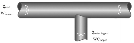
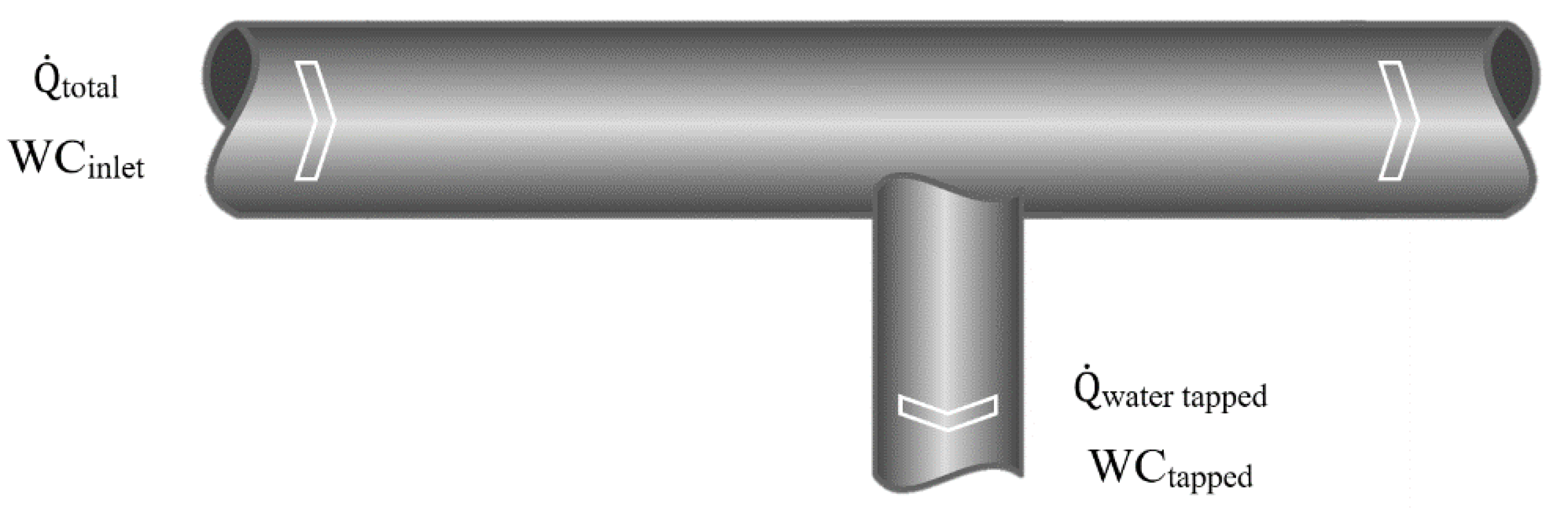
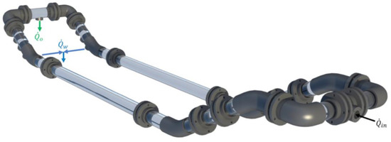
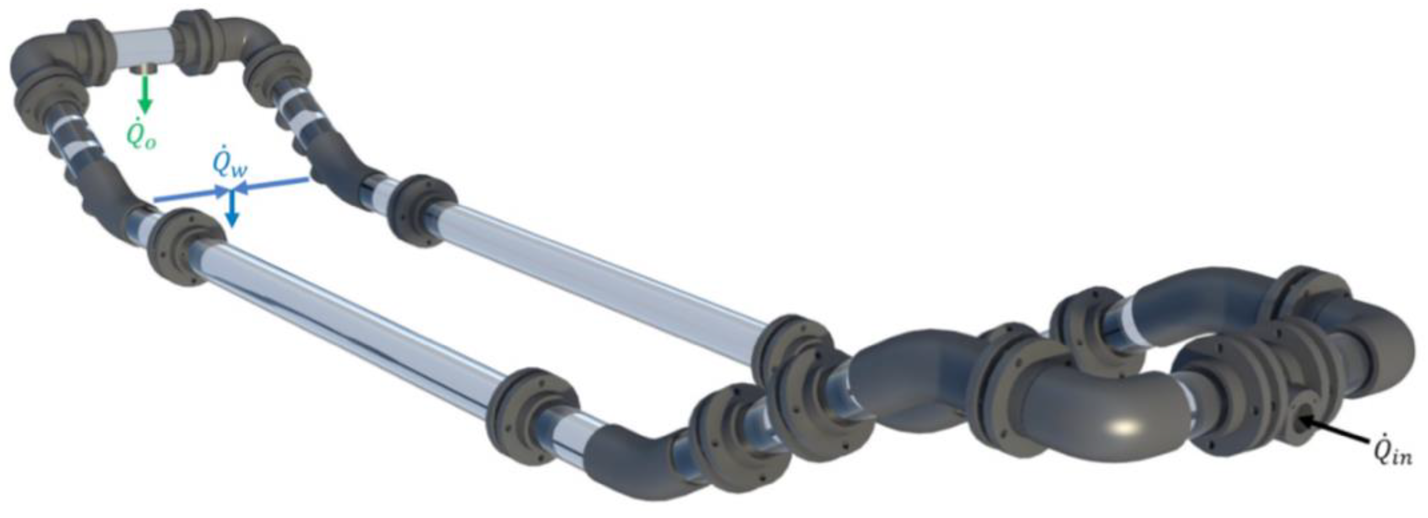
Consider the oil–water separation configuration shown in Figure 1, in which a mixture of oil and water with a total liquid flow rate of total and water flow rate of water enters the separator. Water and some oil are removed through the tapping point pointing downwards, while an oil-rich stream exits towards the right. The tapped stream has a water rate of water tapped, a total tapped liquid flow rate of total tapped and a water fraction (also called water cut) equal to WCtapped. The pipe can be horizontal or have an upward or downward angle with respect to the horizon.
Figure 1.
Tapping of stream.
The efficiency of the tapping point can be expressed by the proportion of the total water flow tapped with respect to the inlet water flow, (WT) as expressed by Equation (1) below:
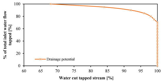
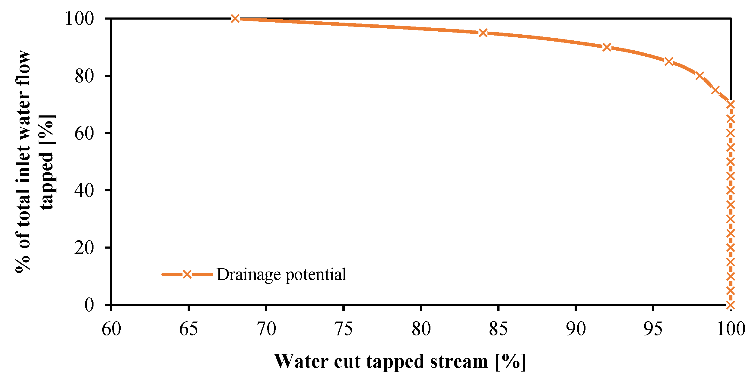
As introduced by Stanko and Golan (2015), the drainage potential curve is the relationship between WT versus WCtapped. This relationship depends on the rates and properties of oil and water, the pipe size, inclination and material, and the location and configuration of the tapping point, among others. An example of a drainage potential curve is given in Figure 2. This curve was taken from Stanko and Golan (2015) and it is calculated from the experimental data of Elseth (2001) (using cross-section profiles of velocity, water, and oil fractions [19]. The calculation procedure is given in Stanko and Golan (2015) [5]. This figure indicates that it is possible to drain approximately 70% of the inlet water rate before starting to drain noticeable amounts of oil.
Figure 2.
Drainage potential curve. Taken from [5].
2.2. Fluid Mixture Properties
2.2.1. Separation Time
The bottle test is often used to estimate separation times and investigate the effect of various agents on breaking or separating emulsions and dispersions. Bottle tests are performed in this study to determine the dispersion separation times of saltwater and Exxsol D60 mixtures with and without crude spiking. Two series of bottle tests were prepared for this purpose. The first series was made from Exxsol D60 spiked with 185 ppm crude and saltwater at ambient temperature (25 °C) with three different water cuts 25, 50, and 75%. The next series had the same conditions except for crude spiking.
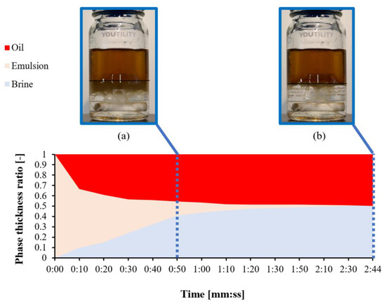
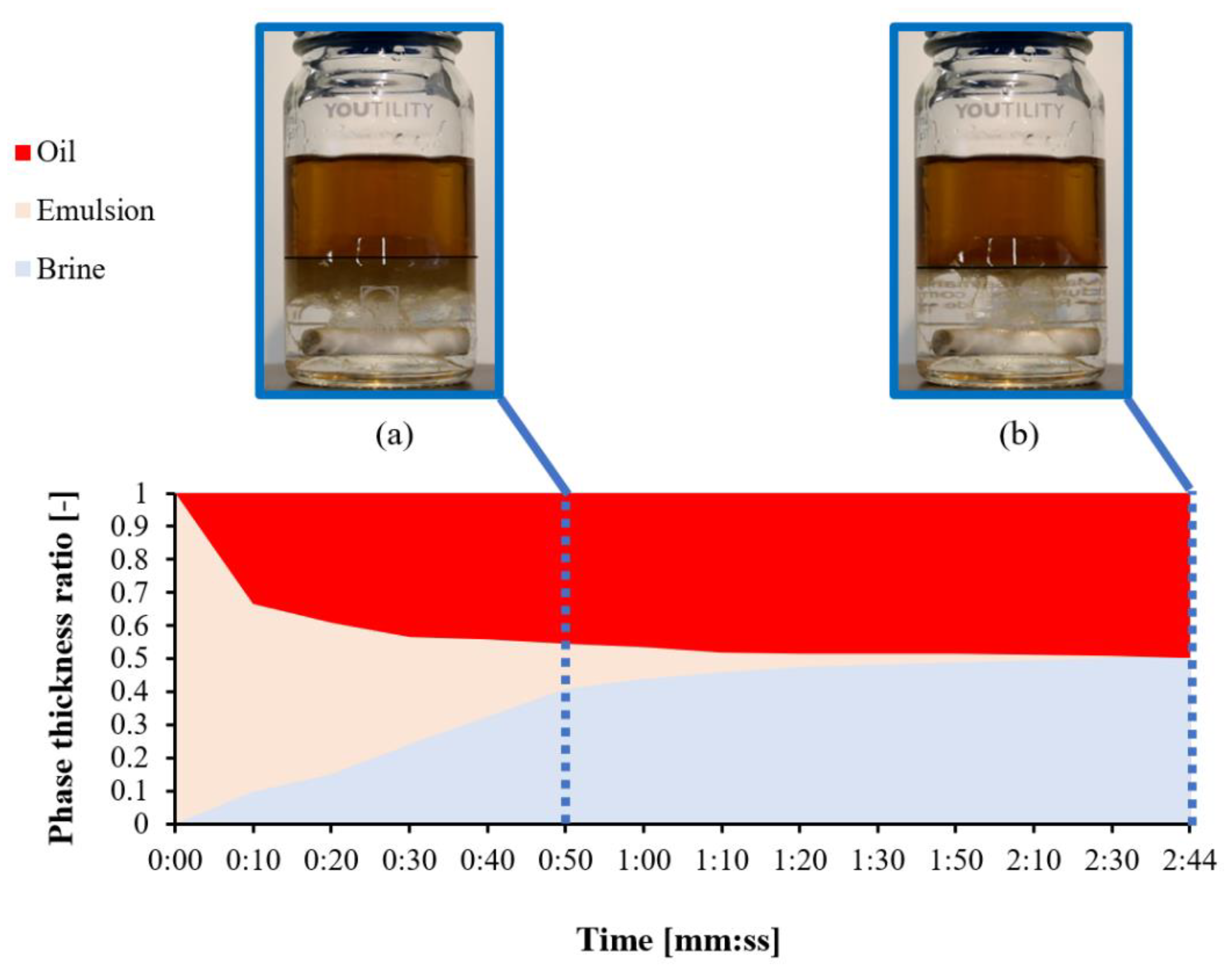
Before giving time for phase separation, the mixture was agitated at 750 rpm for 30 s. The separation process was filmed three times for each sample and then analyzed. The data were split into two time periods. After the magnetic mixer has ceased swirling, the interface between Exxsol D60 and saltwater takes a certain time to become stabilized in the container at a specific height. This time is called tin in this study. The time between the end of mixing and the complete separation of the two layers is called tsep (Figure 3).
Figure 3.
Separation bottle depicting Exxsol D60 with crude oil, WC 50%—conditions of test bottle at (a) tin and (b) tsep.
2.2.2. Inversion Point
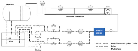
A pipe circulation setup was used as a flowing rheometer to study the emulsion characteristics, effective viscosity, and inversion point. The experiments were carried out in the SINTEF Multiphase Flow Lab’s mini-loop setup in Tiller, Norway. Figure 4 depicts a comprehensive sketch of the test section. The horizontal test section is 2 m long and has an inner diameter of 8 mm. It is made of stainless steel and is fully insulated. Initially, a 1 m3 storage tank was filled with distilled saltwater, and Exxsol D60 in equal portions. Liquids were pumped separately from the tank before being mixed at the test section inlet. The liquids were circulated using centrifugal pumps. Before the mixing section, the flow rate of each liquid was also monitored. Valves were also placed to manage the total system pressure and the flow rate of each liquid. In addition, pressure transmitters were employed to measure the pressure drop across the horizontal test section. The second test campaign was performed by adding spiking crude into the main tank.
Figure 4.
Test mini-loop map.
2.3. Draining Potential Measurment
2.3.1. Experimental Facilities
The experimental facilities and setup used in this work are the same as the ones built and used by Skjefstad (2019). The full details are provided in the article by Skjefstad (2019), but some details are repeated here for clarity [2].
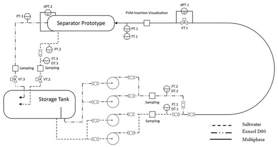
A process and instrumentation diagram of the experimental facilities is presented in Figure 5. There is a large storage tank (total liquid volume of 6 m3) that also provides baseline separation, two small and two large centrifugal pumps, piping, valves, and pressure and flow meters. Water and oil streams are drained separately from tap points in the storage tank, pumped, flow rates are measured, and then the streams are merged into a single flowline. The mixture then enters a control valve (VT.1, in these experiments always open), and subsequently, the separator prototype separates a water-rich stream and an oil-rich stream. The two streams are then directed to the storage tank using two flow lines.
Figure 5.
PI&D of the experimental system setup.
The inlet oil and water rates and water cut are adjusted by controlling the frequency of the pumps. The rates of the separated streams can be adjusted by gradually opening or closing the control valves located at the separator outlets (VT.3 and VT.2).
Pressure is measured across the inlet control valve (VT.1), at the inlet, and at outlets of the separator. The flow rates and water cuts of oil and water are measured with Coriolis flowmeters before the merging point and at the water-rich stream downstream of the separator.
The design has been optimized in terms of the inclination of the extraction section, and the configuration of the inlet device. Skjefstad (2019) performed experiments were conducted with 30°, 45°, and 60° upwards inclination and reported results displayed the best separation efficiency for 30° inclination [20]. The separator consists of two parallel pipes that have an inclined downwards section, a horizontal section (approximately 3.5 m long), and an upwards inclined section as presented in Figure 6. The total projected horizontal length of the separator is 6.1 m. At the inlet splitting section, it is possible to install different types of flow inlet sections to alter the distribution of the flow. In this study, all experiments were performed using a tangential pipe inlet. Because of this tangential inlet, the water will be pushed towards the pipe wall, while the less dense oil will be grouped in the pipe center. This annular configuration is then redirected into a layered flow distribution using a flow redistribution device installed in the elbow at the start of the downwards inclined section. More details about the inlet configuration and redistribution device can be found in Skjefstad and Stanko (2018) [11]. Phase segregation occurs in the horizontal section. The flow is photographed at the end of the horizontal section. The tapping of the water-rich phase is performed at the beginning of the upwards inclined section. The goal of the inclined extraction section is that the water layer at the bottom of the pipe would be slowed down, reducing its velocity, increasing the layer height, and making it easier to tap without generating much turbulence and mixing. The water-rich separated streams are then merged. The oil-rich streams are also merged. The separated streams are then sent to the storage tank.
Figure 6.
Prototype of parallel pipe bulk oil–water separator.
The storage tank was originally filled with equal amounts of distilled water with 3.4 wt% NaCl and Exxsol D60 with 0.015 gr/L of the colorant Red O (C26H24N4O).
2.3.2. Experimental Campaign
Drainage potential curves of the tapping points were generated by fixing the inlet conditions (total flow rate and water cut) and varying the amount of water drained through the tapping point by adjusting control valves VT.3 and VT.2. Experiments were conducted with the unspiked Exxsol D60 and water and later with spiked Exxsol D60 and water. Table 1 presents the test range in terms of inlet flow rate, WCinlet, and water tapped (WT). However, it was not possible to do all combinations presented in the table due to limitations of the pumps’ capacities at high total rates. The ultimate combinations tested are presented in Table 2 and Table 3.
Table 1.
Unspiked Exxsol D60 Experimental campaign test matrix.
Table 2.
Unspiked Exxsol D60 Experimental campaign infill test matrix.
Table 3.
Spiked Exxsol D60 Experimental campaign infill test matrix.
2.3.3. Testing Procedure
Using LabVIEW’s operation panel, the inlet liquid flow rate and WCinlet are set. Some time is given for the system to reach stable conditions. Then control valves VT.2 and VT.3 are automatically adjusted to achieve the desired WT. The WT was calculated from the water cut of the water stream at inlet (WC1), the flow rate of water at inlet (), water cut of Exxsol stream at inlet (WC2), flow rate of oil at inlet (), WCtapped (WC3) and tapped flow rate (), as shown in Equation (2):
After the system reaches steady state, measurements are then taken; 300 individual measurements are recorded with a sampling frequency of 10 Hz. Flow patterns are photographed at this time.
2.4. Drainage Potentia—Numerical Estimation
A numerical model was developed to estimate the drainage potential curve when tapping from a single tapping point. The input to the model is the inlet volumetric rates of oil and water, the pipe diameter, the type of flow pattern existing in the pipe, and some parameters needed depending on the flow pattern type. The flow patterns considered are based on the work by Trallero et al., (1997) and have two or three layers [21]:
- Two-layer regimes: O & W, Dw/o & Do/w, O & Do/w, Dw/o & O. For these flow patterns a WiO content must be provided for the oil dominated layer and an OiW for the water dominated layer.
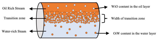
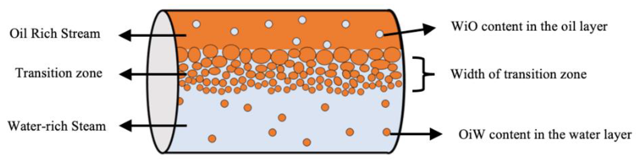
- Three-layer regimes: O & Dw/o (or Do/w) & W. For these regimes the thickness of the middle layer must be provided and the OiW content in the W layer and the WiO content in the O layer. The water fraction in the middle layer is assumed to vary linearly.
Appendix A contains more information about the flow regime acronyms used above.
The model consists of two steps:
- 1
- With the input provided perform an iterative solving process to compute the height of each layer and the distribution of the water volume fraction along the vertical axis (). In this iterative solving process, the convergence criteria consist of obtaining the same water cut value that is input via integration of the water volume fraction profile. The number of discretized points in the pipe are selected such as the value of the cross-section area obtained by integration which gives the same results as the actual pipe cross section area. The fluid velocity is assumed to be uniform in the cross-section and equal to the mixture velocity.
- 2
- Compute the production potential curve using the distribution provided:
- (a)
- Define a generic height “h” to drain
- (b)
- Compute, integrating numerically , the oil and water rates in the region between the pipe bottom to the height “h”
- (c)
- Compute WT and WCtapped with the oil and water rates in the tapped region
- (d)
- Steps a–c are repeated several times for several “h” values from zero to the pipe diameter.
More details about the model and the solving process are provided in Appendix B.
3. Results
3.1. Fluid Dispersion Properties
3.1.1. Separation Time
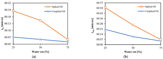
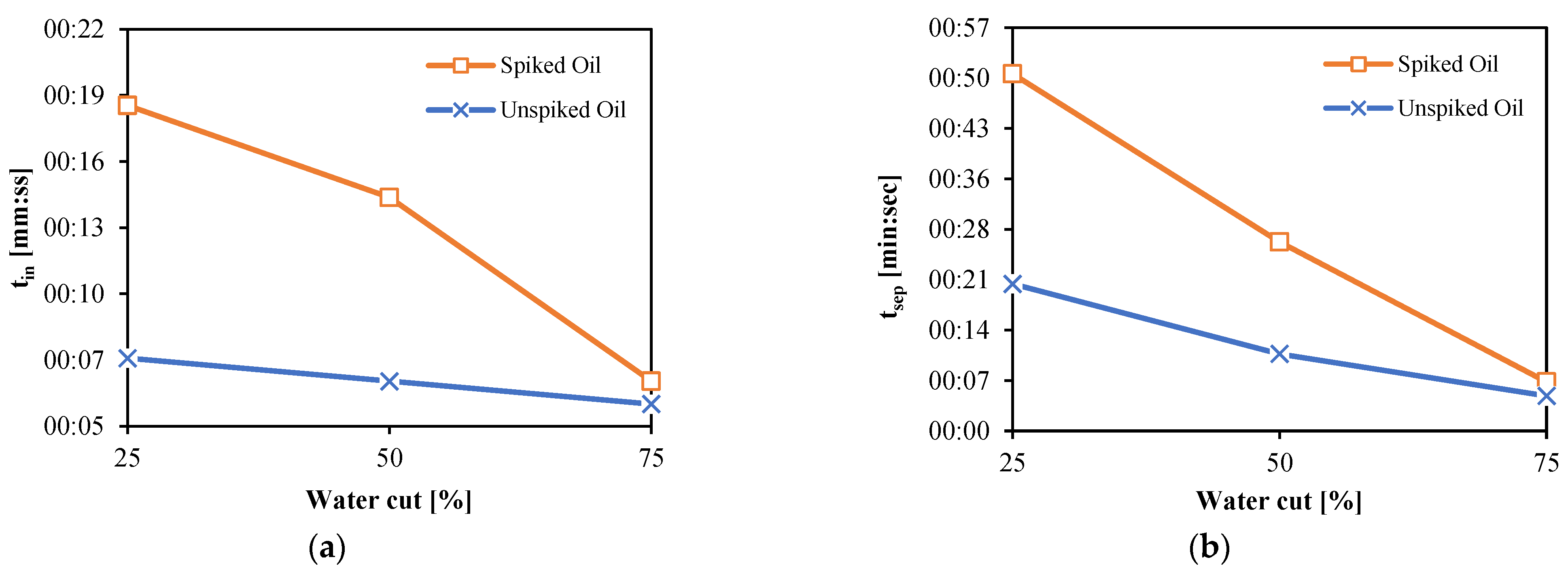
Separation times for dispersions of Exxsol D60 (denoted as unspiked oil) and Exxsol D60 + 185 ppm crude oil (denoted as spiked oil) with saltwater were measured by bottle test. Figure 7a,b illustrates separation times (tin and tsep) of dispersion samples with three different water cuts of 25, 50, and 75%. All curves have a descending trend when the water cut is increased from 25 to 75%. Generally, dispersions of spiked oil require higher separation times when compared with unspiked oil dispersion, although, the difference in their separation times is not significant at a water cut of 75%.
Figure 7.
(a) Required time for fixed interface, tin, and (b) required time for phase separation, tsep versus water cut.
3.1.2. Inversion Point
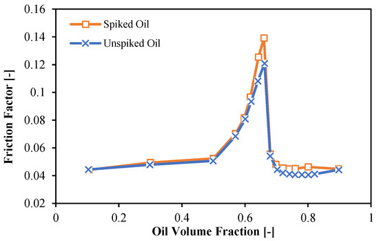
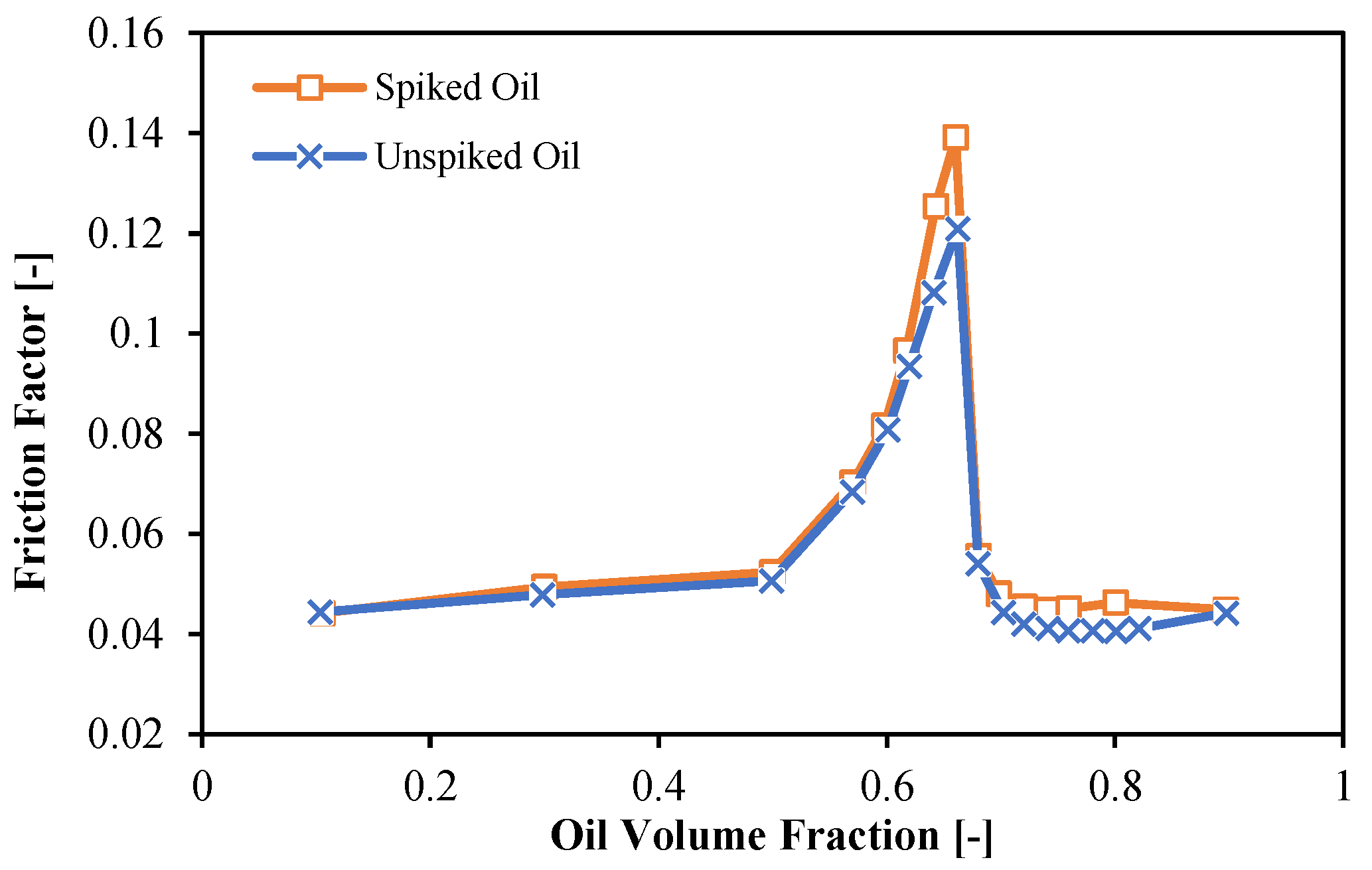
Figure 8 shows the friction factor of dispersed flows with different values of oil volume fraction, back calculated from pressure drop measurements across the pipe. Results show the dispersion of spiked oil with salt water has a higher friction factor than the dispersion of unspiked oil in the region close to the inversion point. Both curves show an inversion point close to the oil volume fraction of 0.66 (approximately equal to 33% water cut).
Figure 8.
Inversion points of spiked oil and unspiked oil dispersions with saltwater at mixture velocity 0.66 m/s.
3.2. Drainage Potential Curve Experimental Results
The drainage potential curve calculated from experimental values is presented in this section. First, the drainage potential curves unspiked oil and spiked oil are shown under the same inlet conditions, i.e., WCinlet and total inlet liquid rate. This illustrates the effect of adding crude oil on the separation performance of the tapping point.
Next, the drainage potential curves are displayed for a fixed inlet WCinlet and a fixed fluid mixture (spiked oil + water or unspiked oil + water) but varying the inlet liquid flow rate. This is to show how the drainage potential curves are affected by changes in the inlet liquid rate and to determine if this behavior depends on the spiking concentration.
The drainage potential curves discussed in this work are computed for the two parallel tapping points. If both tapping points behave identically, then they should have the same drainage potential curve.
3.2.1. Comparison between Drainage Potential Curves for Unspiked Oil and Spiked Oil at the Same Inlet Conditions
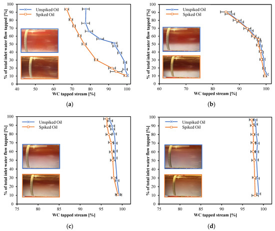
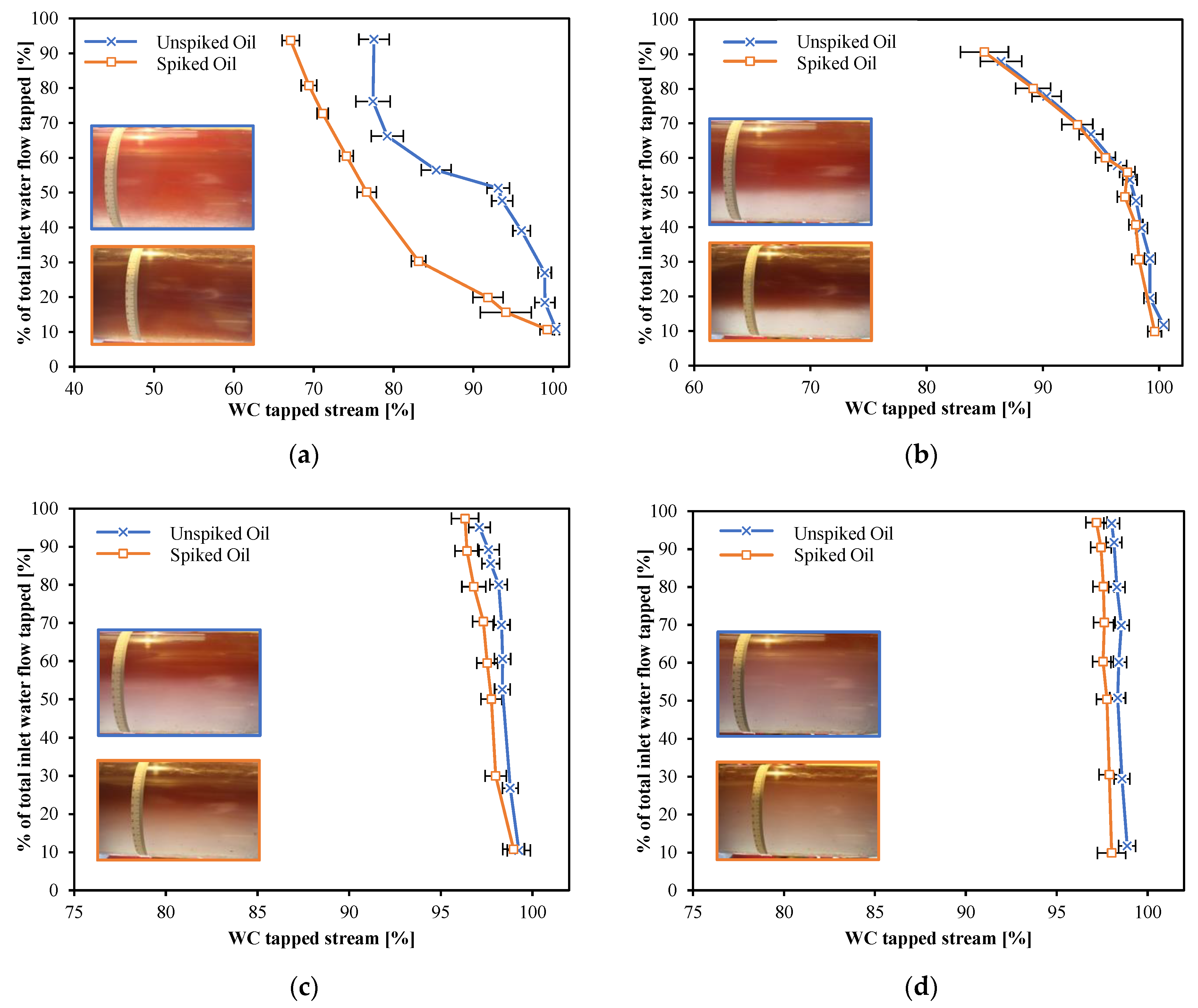
Figure 9 shows the drainage potential curves for a total flow rate of 300 L/min and WCinlet values of 30% (Figure 9a), 50% (Figure 9b), 70% (Figure 9c), and 90% (Figure 9d) for the spiked and unspiked oil. Figure 9d also includes some photos of the flow pattern upstream of the tapping point.
Figure 9.
Drainage potential for spiked oil and water and unspiked oil and water with total flow rate of 300 L/min, at WCinlet (a) 30%, (b) 50%, (c) 70%, and (d) 90%.
For all these cases, it is possible to tap large amounts of water without tapping large amounts of oil. For WCinlet values between 50–90%, it seems no significant amounts of oil are tapped until 90% of the inlet water stream is tapped (the curve is fairly vertical). However, for a WCinlet of 30%, the threshold WT at which oil starts to be tapped is much lower (around 30%). The drainage potential curves are very similar between the unspiked oil and spiked oil, exhibiting the largest differences at the WCinlet value of 30%. For a WCinlet of 30%, the decrease in WC of the tapped stream versus WT is sharper for the spiked oil than for the unspiked oil.
For all the conditions presented in Figure 9d, the flow pattern approaching the tapping point is O & W and there are no noticeable dispersion layers. This could be the reason why it is possible to drain significant amounts of water without dragging oil through the tapping point and why the spiking does not have a big impact on the drainage potential.
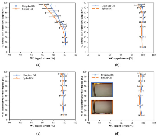
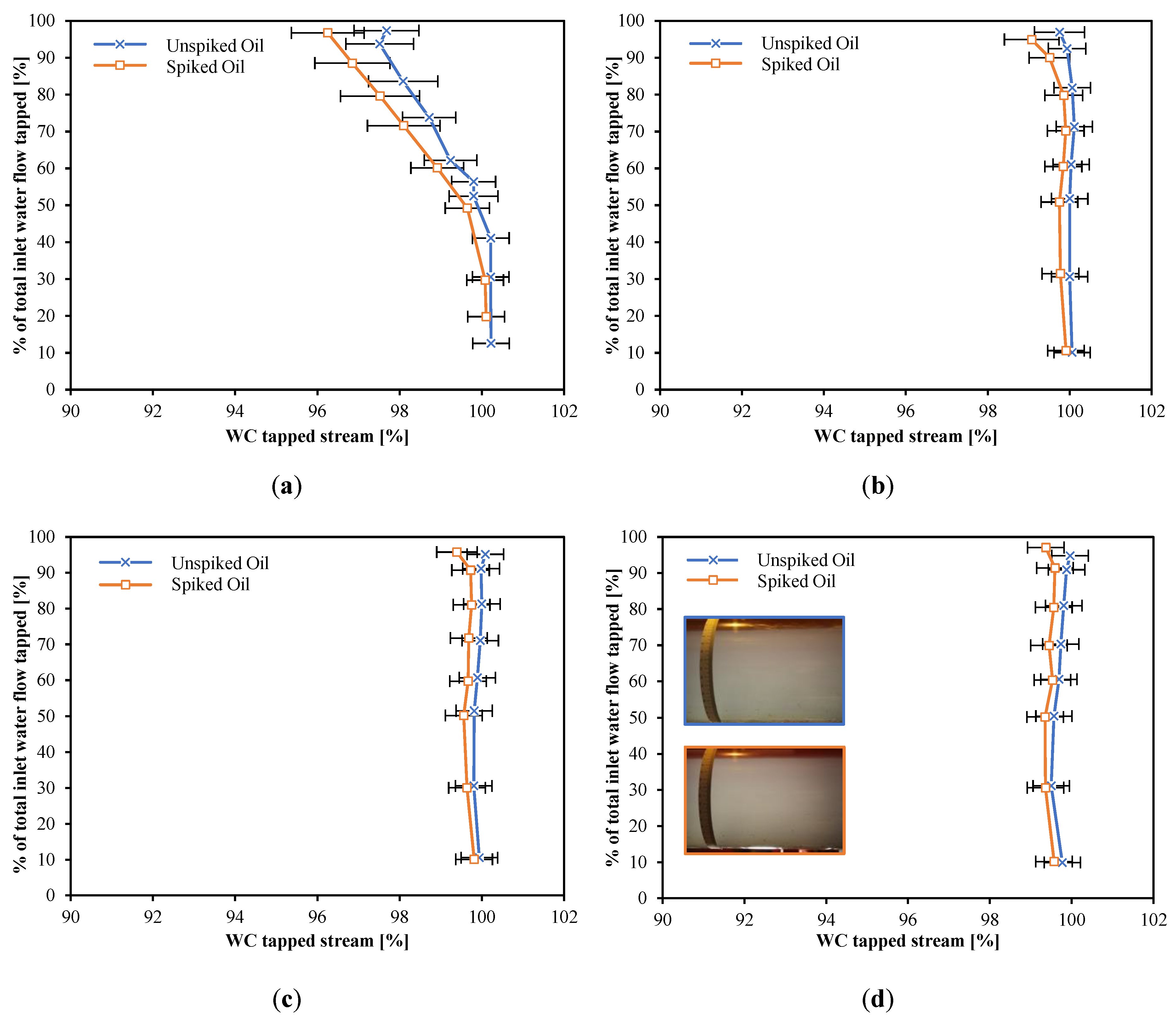
Figure 10 shows the drainage potential curves for a total flow rate of 500 L/min and WCinlet values of 30% (Figure 10a), 50% (Figure 10b), 70% (Figure 10c), and 90% (Figure 10d) for the spiked and unspiked oil. Figure 10 also includes photos of the flow pattern upstream of the tapping point. For WCinlet values of 70 and 90%, the amount of oil tapped is low up to WT values of 90%. The photos indicate that the flow pattern approaching the tapping point consists of O&W with a thick water layer, therefore it seems that most of the water is transported in this layer and is tapped from it.
Figure 10.
Drainage potential for spiked oil–water and unspiked oil–water with total flow rate of 500 L/min, at WCinlet (a) 30%, (b) 50%, (c) 70%, and (d) 90%.
For WCinlet values of 30 and 50%, the drainage potential curves exhibit a decline in the water cut of the tapped stream with an increase in WT. For a WCinlet equal to 50%, the decline is sharper after WT surpasses 50%. According to the photo, the flow pattern approaching the tapping point seems to be O & Dw/o & W. Because the water cut of the tapped stream declines at WT greater than 50%, it seems to indicate that the rest of the water is transported as a dispersion in the oil.
There were no big differences between the drainage potential curves of the spiked and unspiked oil, except for the WCinlet value of 30%. Here, the flow regime is O & Dw/o & Do/w. For the spiked oil the Do/w region is diminished when compared to the unspiked oil, which might explain the poorer drainage potential, i.e., the crude oil spiking increases the amount of oil dispersed in the water layer close to the bottom of the pipe. This is consistent with the observations provided by Kokal (2008), i.e., adding crude to Exxsol D60 may result in more stable emulsions due to the heavy polar components in the crude [22].
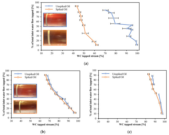
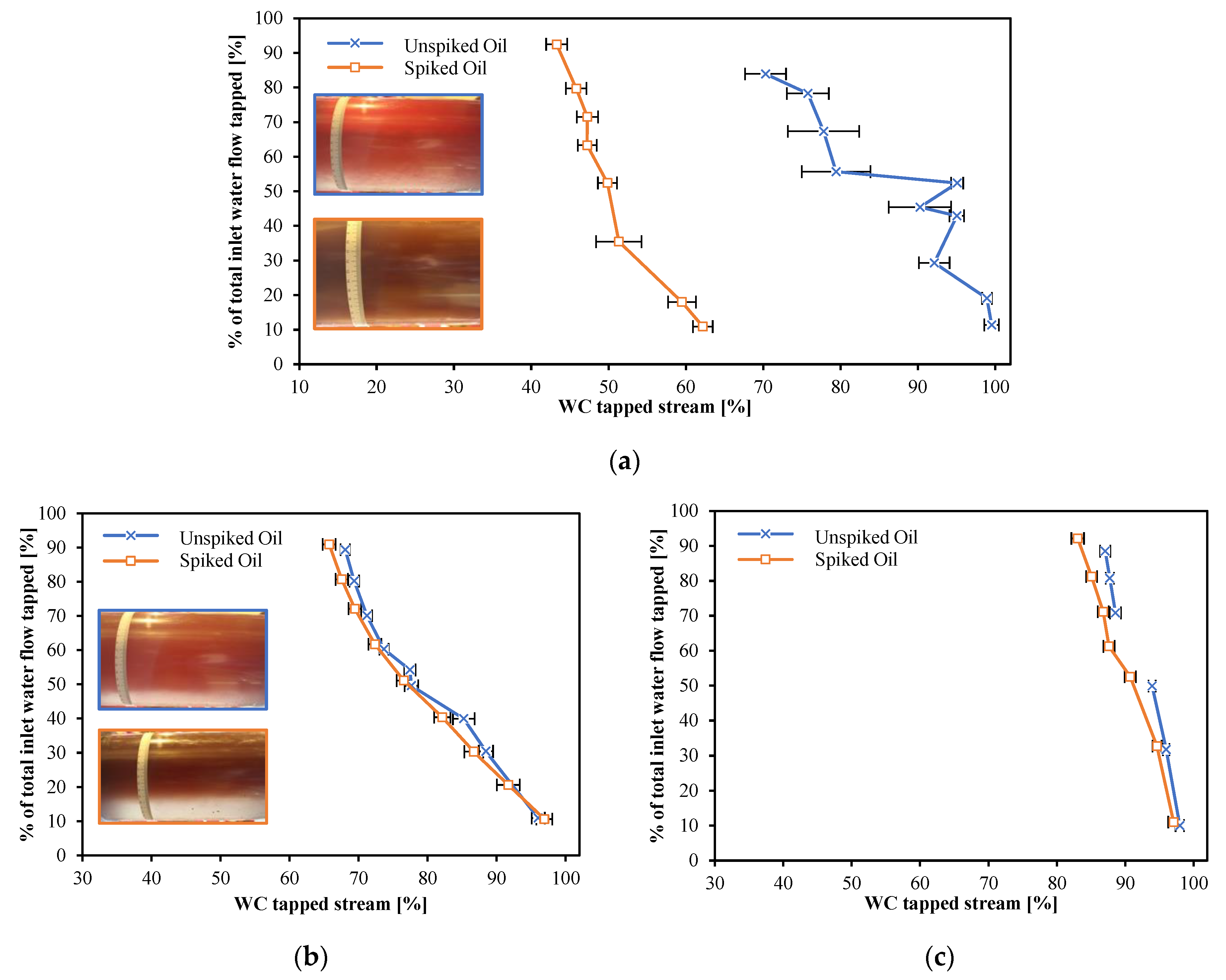
Figure 11 shows the drainage potential curves for a total flow rate of 700 L/min and WCinlet values of 30% (Figure 11a), 50% (Figure 11b), and 70% (Figure 11c) for the spiked and unspiked oil. Figure 11 also includes some photos of the flow pattern upstream of the tapping point.
Figure 11.
Drainage potential for spiked oil and water and unspiked oil and water with total flow rate of 700 L/min, at WCinlets (a) 30%, (b) 50%, and (c) 70%.
There were no significant differences between the drainage potential curves of the spiked and unspiked oil, except for the WCinlet value of 30%. Here, for the unspiked oil the flow regime is O & Dw/o & Do/w. For the spiked oil, the Do/w region almost disappears, which might explain the poor drainage potential. For all cases the drainage potential curves exhibit a steady decline in the water cut of the tapped stream with an increase in WT.
For a WCinlet equal to 50%, the flow pattern approaching the tapping point seems to be O & Dw/o & W. However, because the water cut of the tapped stream declines steadily with WT it seems to indicate that the amount of water transported by the clean water layer is small and the rest is transported as a dispersion in the oil.
3.2.2. Behavior of Drainage Potential Curves with Total Flow Rate at Fixed WCinlet and Same Fluid Mixture
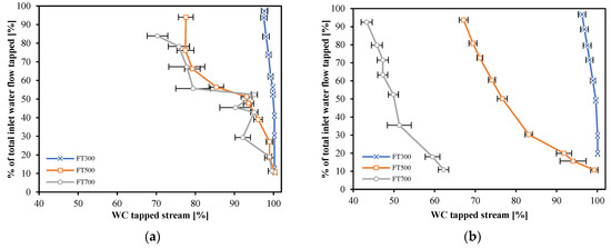
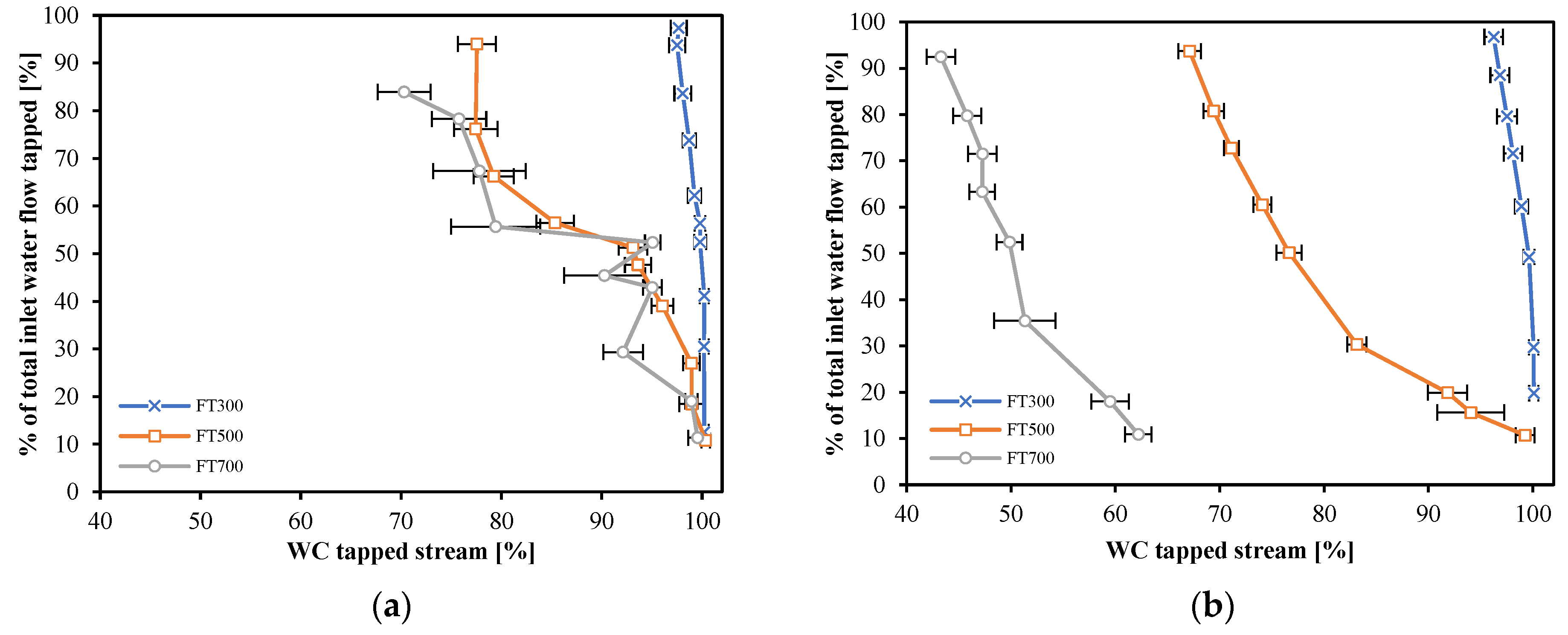
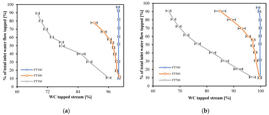
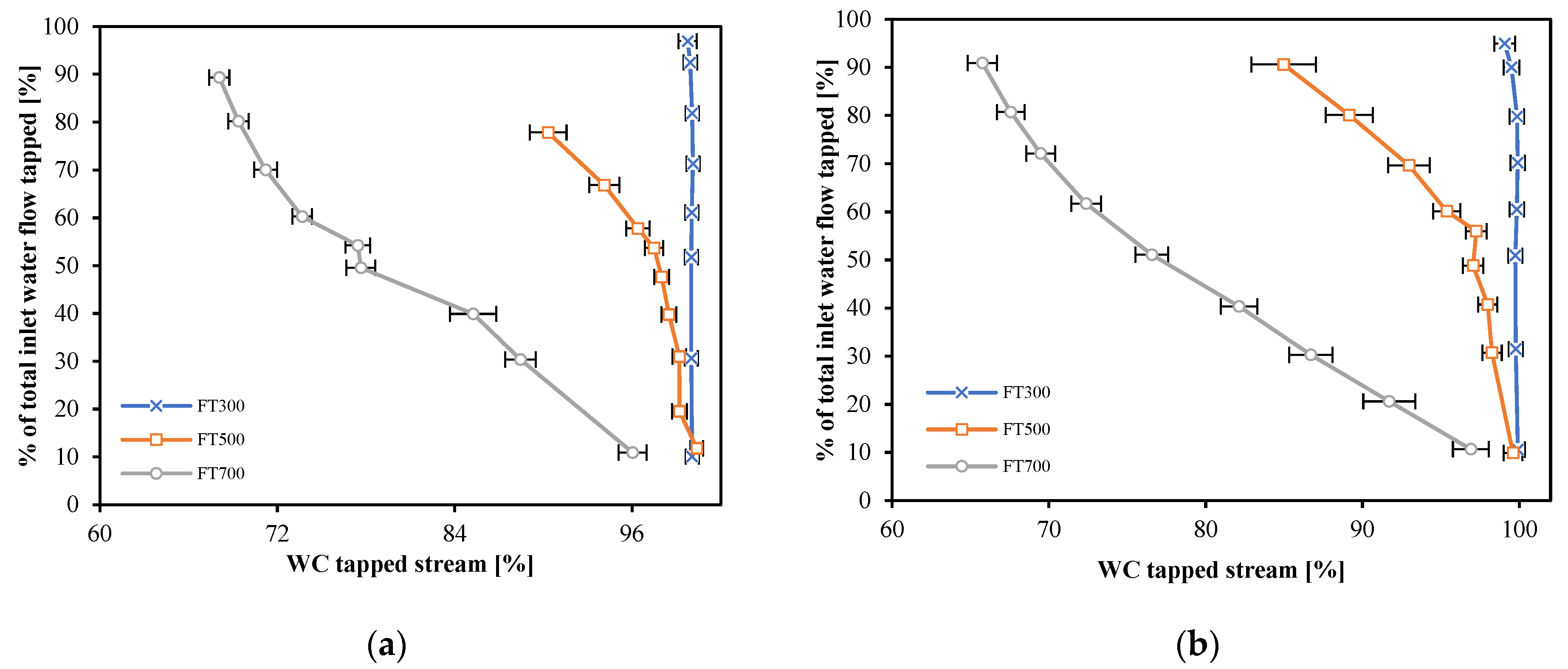
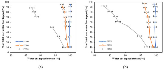
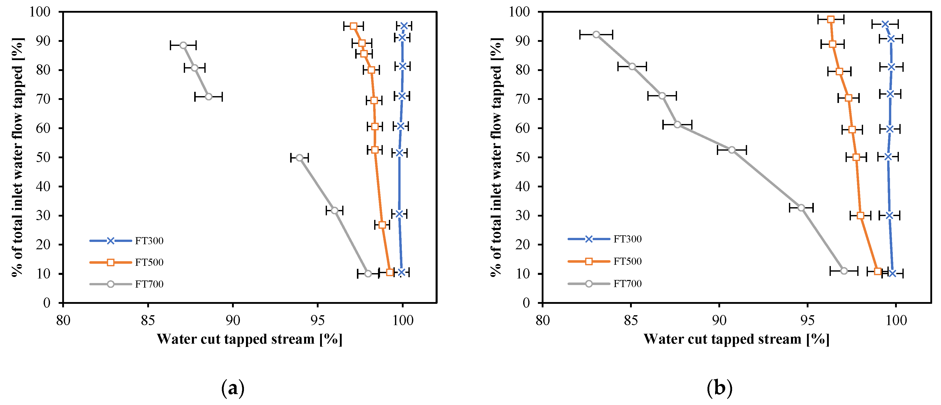
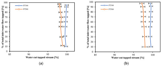
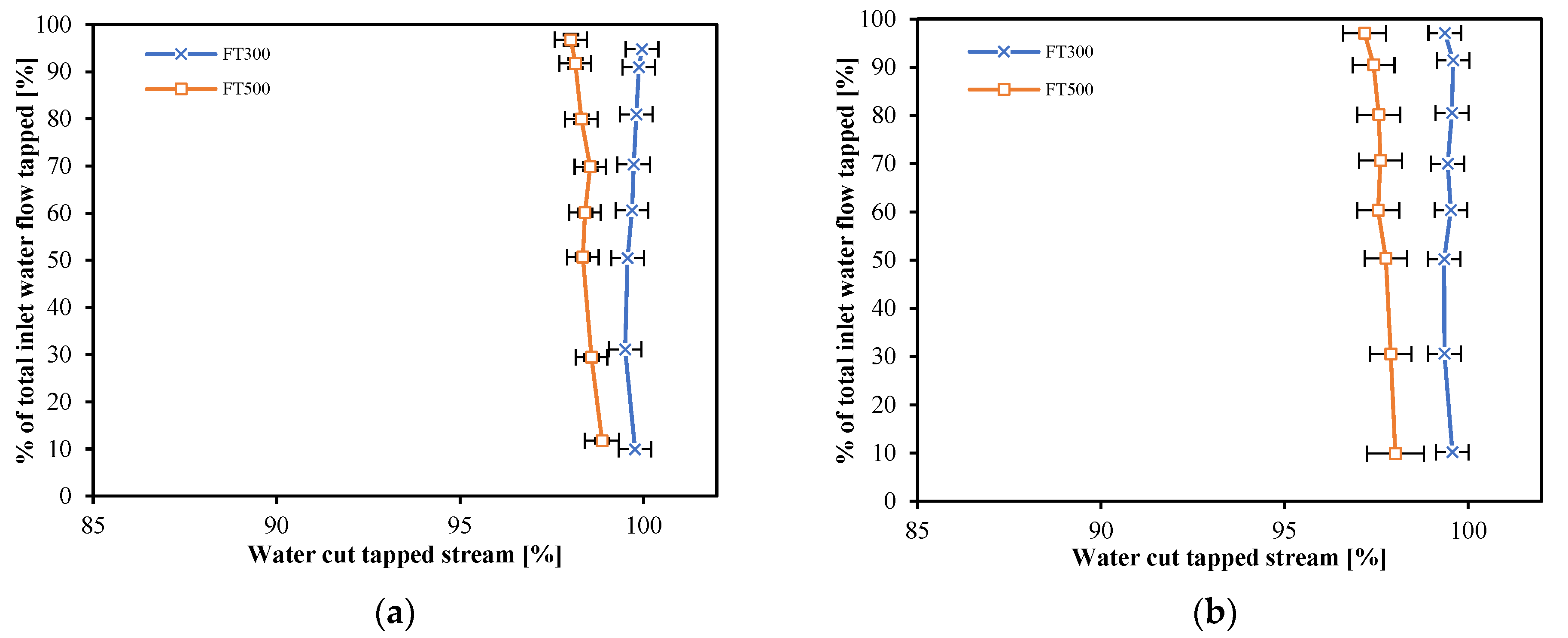
Figure 12, Figure 13, Figure 14 and Figure 15 show drainage potential curves for WCinlet equal to 30%, 50%, 70%, and 90% respectively. Each figure has drainage potential curves for flow rates of 300, 500, and 700 L/min and for unspiked (version a) and spiked crude (version b). The same trend is observed in all figures: higher flow rates are detrimental to drainage potential performance.
Figure 12.
Drainage potential for (a) unspiked, (b) spiked oil and water at WCinlet 30%, total flow rate of 300, 500, and 700 L/min.
Figure 13.
Drainage potential for (a) unspiked, (b) spiked oil and water at WCinlet 50%, total flow rate of 300, 500, and 700 L/min.
Figure 14.
Drainage potential for (a) unspiked, (b) spiked oil and water at WCinlet 70%, total flow rate of 300, 500, and 700 L/min.
Figure 15.
Drainage potential for (a) unspiked, (b) spiked oil and water at WCinlet 90%, total flow rate of 300, and 500 L/min.
3.3. Drainage Potential Curve—Numerical Modeling Results
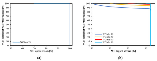
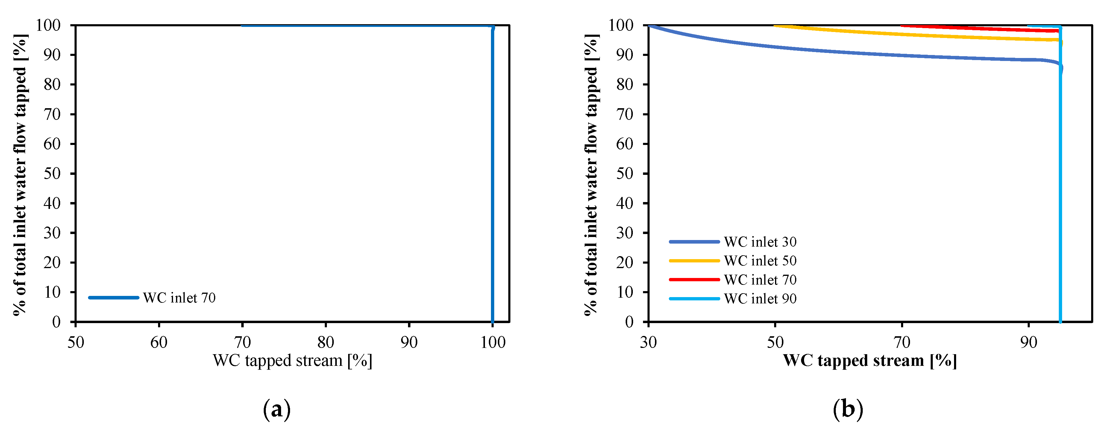
Figure 16 shows the drainage potential curve generated numerically for several flow patterns. Figure 16a shows the curve for a WCinlet 70%, assuming an O & W flow pattern. The curve is vertical, and very similar to the experimental results with WCinlet values of 70% and 90% and total flow rate of 300 L/min. Figure 16b shows drainage potential curves for Dw/o & Do/w, with water fraction in the oil (WiO) equal to 5%, and oil fraction in water (OiW) equal to 5% and WCinlet values of 30%, 50%, 70%, 90%. Because of the presence of the dispersed phase, the drainage potential curve does not cross the x axis at 100%, but at 95% WCtapped. The WCtapped remains constant with WT until the layers’ interphase is reached, where it drops sharply with WT. These sharp declines were not observed in the experimental data. In the experimental data, when the flow pattern exhibited an apparently clean water layer at the pipe bottom, the x-axis intersection was not always located at 100%, but less. This indicates there is some oil present in the water layer.
Figure 16.
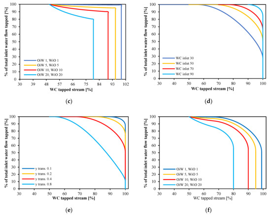
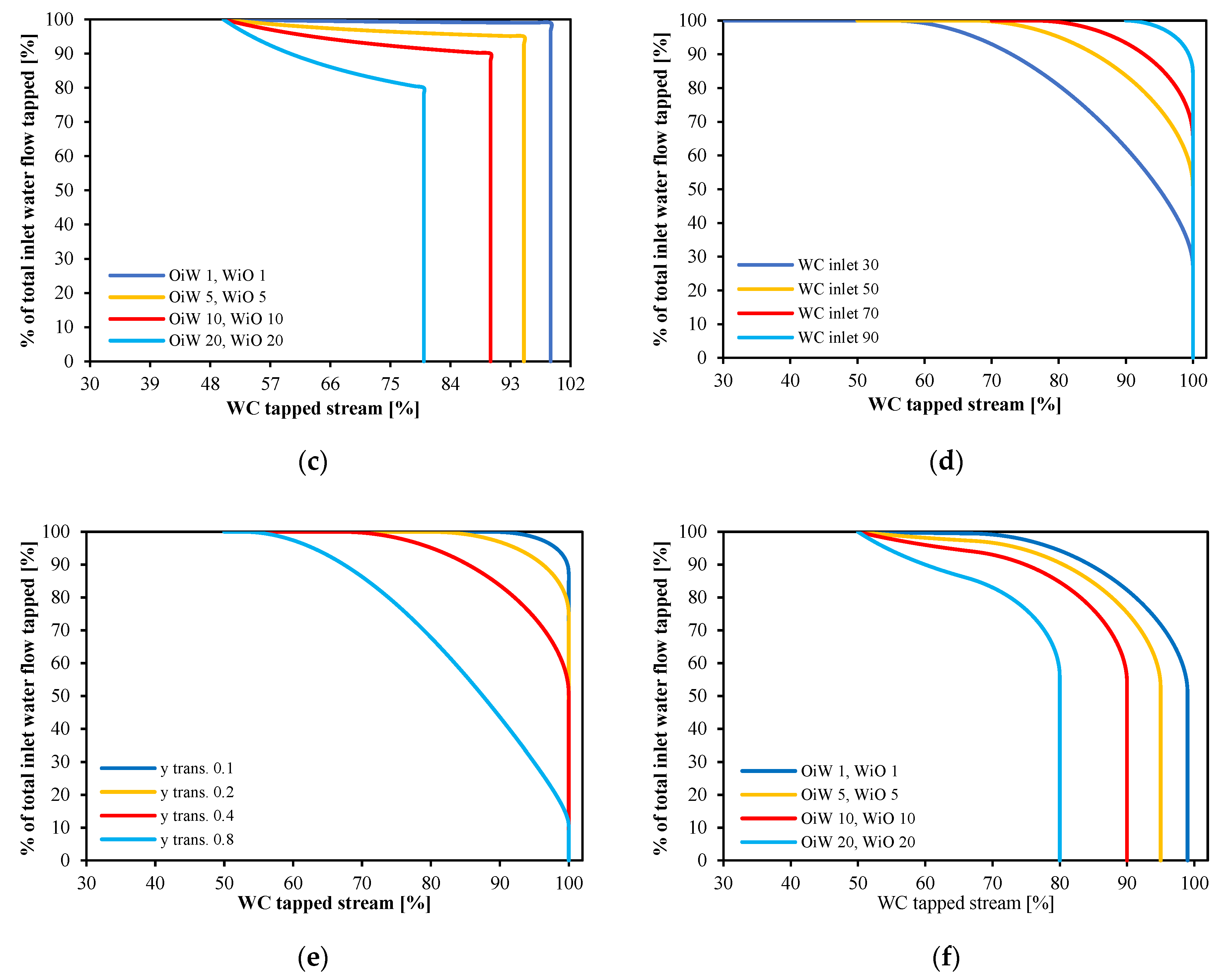
Model prediction of drainage potential curve for a certain (a) step volume fraction of water and WC inlet 70%, (b) step volume fraction of water with 5% uniform contamination of WiO and OiW and various WCinlet 30%, 50%, 70%, 90%, (c) step volume fraction of water with different uniform contamination 1, 5, 10, and 20% of WiO and OiW, WCinlet 50%, (d) linear water volume fraction change in phase distribution of transition zone with 0.4 normalized width for four different WCinlet 30%, 50%, 70%, 90%, (e) linear water volume fraction change in phase distribution of transition zone with different normalized width 0.1, 0.2, 0.4, 0.8 WCinlet 50%, (f) linear water volume fraction change in phase distribution of transition zone with normalized width of 0.4 and uniform contamination 1, 5, 10, and 20% of WiO and OiW, WCinlet 50%.
Figure 16c shows drainage potential curves for Dw/o & Do/w with different combinations of water fraction in the oil (WiO) and oil fraction in water (OiW) from 1 to 5, 10 and 20% dispersed phase fraction and WCinlet value 50%. The higher the OiW, the lower the value of WCtapped on the x axis. The higher the WiO, the less sharp is the decline in WCtapped after the layers’ interphase is reached. The numerical curve at the highest WiO resembles the curve for the case of total flow 500 L/min and WCinlet equal to 50%, which makes sense considering the photographed flow pattern is O & Dw/o & W. Figure 16d,e shows drainage potential curves estimated assuming a flow pattern O & o/w & W. The water volume fraction is assumed to change linearly from 1 to 0 in the o/w later. Figure 16d assumes that the thickness of the o/w layer is 0.4 times the diameter with WCinlet values of 30%, 50%, 70%, 90%. In Figure 16e, several thicknesses of the o/w layer were tested (expressed in fraction of the pipe diameter) and a WCinlet equal to 50%.
Figure 16f shows drainage potential curves estimated assuming a flow pattern O & o/w & W, with different combinations of water fraction in the oil (WiO) and oil fraction in water (OiW). The water volume fraction is assumed to change linearly in the o/w later from the OiW to the WiO values. The thickness of the o/w layer is 0.4 times the diameter and the WCinlet is 40%. In general, Figure 16d–f shows a WT vs WCtapped behavior similar to the one observed in some experimental conditions (above a limit, increasing WT leads to decreased WCtapped), but with a different curve concavity. The numerical curve is concave, while the experimental are usually linear or slightly convex. This could indicate that in the flow patterns observed experimentally, the dispersed oil/water layer exhibits a uniform water volume fraction versus height, or a slightly increasing water volume water fraction in height instead of a decreasing water volume fraction in height.
4. Discussion
4.1. Model Validation
Model-generated drainage potential curves for three sets of data are presented in this section. Then, the acquired experimental data are used to validate the proposed simplified model. The Model considers that the phase distribution of pipe cross-section is a three-layer regime: O & Dw/o (or Do/w) & W as it is shown in Figure 17. The required model inputs for each condition, the normalized width of transition zone, and the OiW content in the W layer and the WiO content in the O layer (contamination fraction), are extracted and estimated from taken photos. Based on model assumptions, the water volume fraction is considered to change linearly from 1 to 0 and the contamination fraction is uniform.
Figure 17.
Phase distribution of pipe cross-section.
The three experimental data sets studied are:
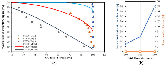
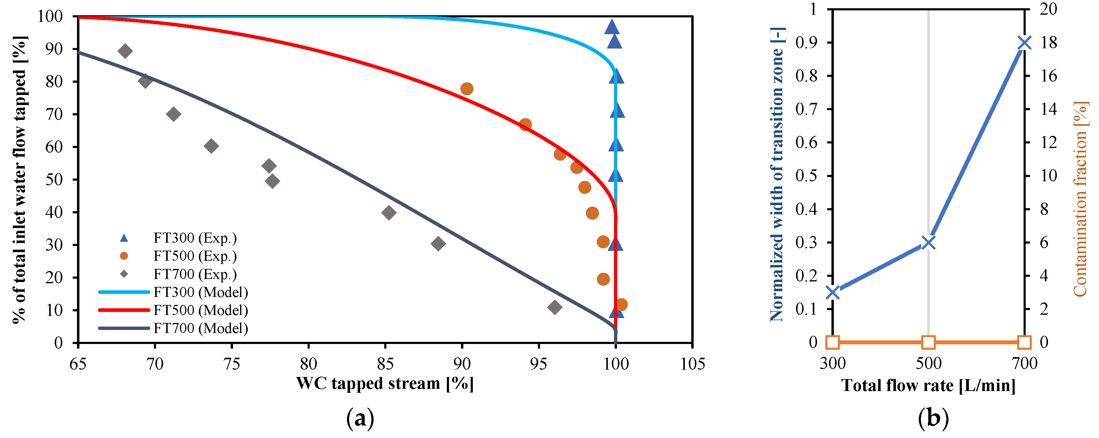
- Unspiked oil with WCinlet 50% for three total flow rates 300, 500, and 700 L/min. The purpose of this data set is to investigate the effect of total flow rate (Figure 18).Figure 18. (a) Comparison between model prediction and experimental data for unspiked oil with WCinlet 50% and total flow rates 300, 500, and 700 L/min, (b) Changes of normalized width of transition zone (blue line) and contamination fraction (orange line) vs. flow rates.
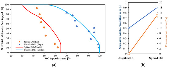
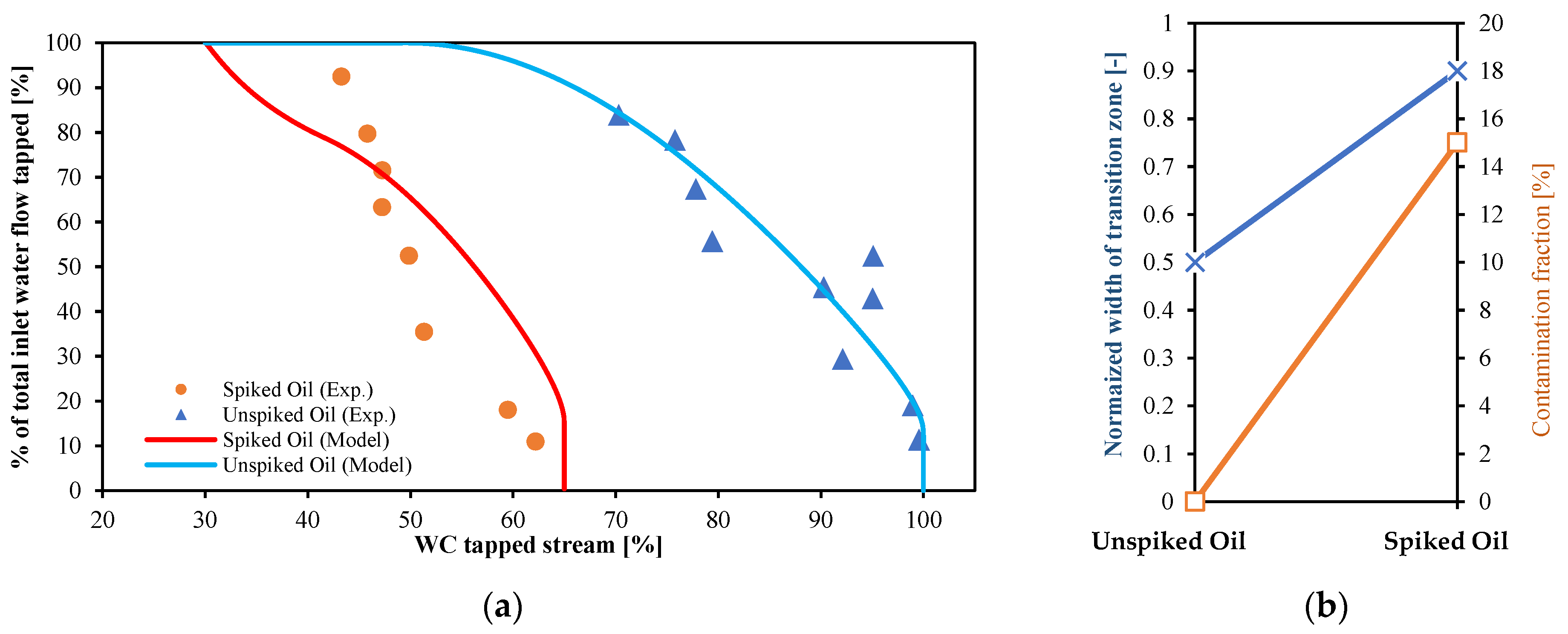
- Spiked and unspiked oils with WCinlet 30% and total flow rate 700 L/min. The purpose of this data set is to investigate the effect of crude spiking (Figure 19).Figure 19. (a) Comparison between model prediction and experimental data for spiked and unspiked oils with WCinlet 30% and total flow rate 700 L/min, (b) normalized width of transition zone (blue line) and contamination fraction (orange line) for spiked and unspiked oil conditions.
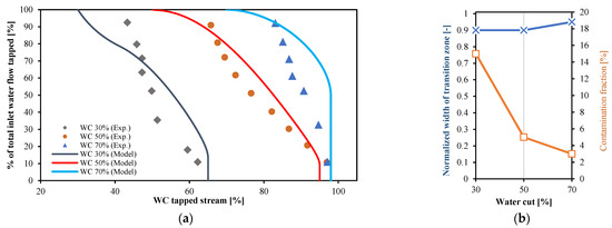
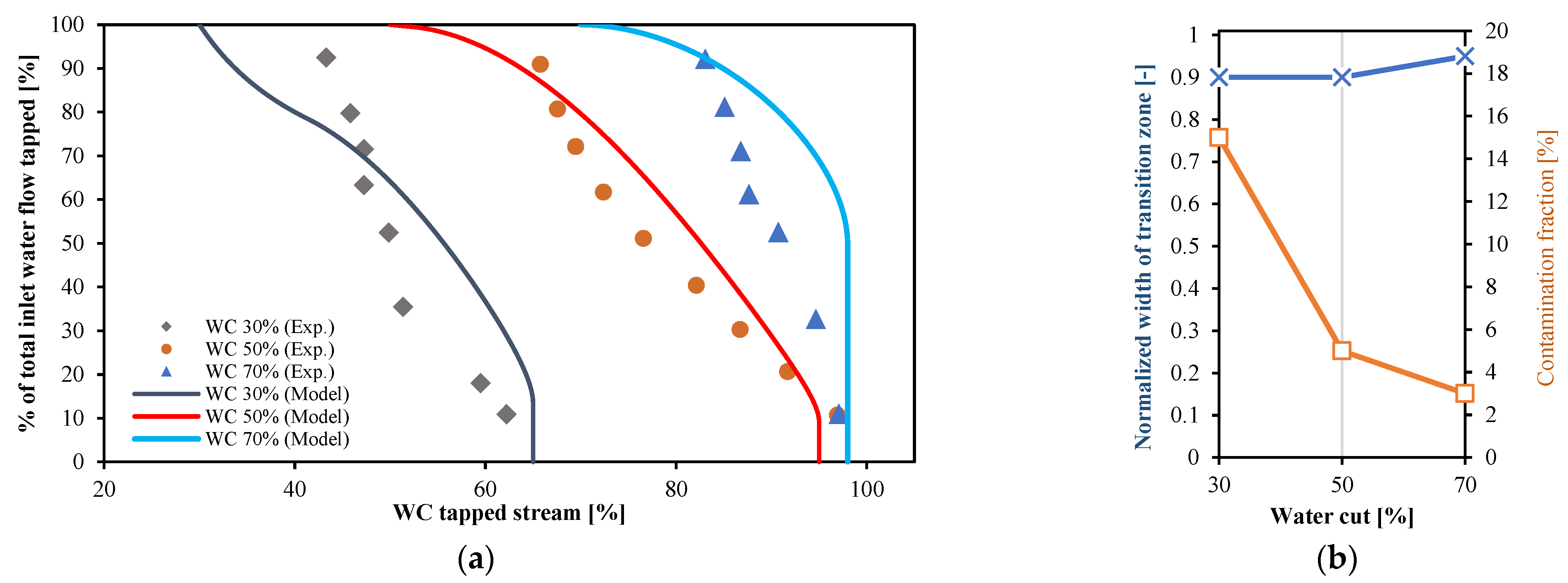
- Spiked oil with total flow rate 700 L/min for three different WCinlets 30, 50, and 70%. The purpose of this data set is to investigate the effect of inlet water cut (Figure 20).Figure 20. (a) Comparison between model prediction and experimental data for spiked oil with total flow rate 700 L/min and WCinlets 30, 50, and 70%, (b) changes of normalized width of transition zone (blue line) and contamination fraction (orange line) vs. WCinlets.
Regarding data set nr. 1, as presented in Figure 18a, the experimental data and model predictions exhibit fair agreement. Keeping the same WCinlet 50% and increasing the total flow rate from 300 to 700 L/min increases the normalized width of the transition zone. There was no significant contamination fraction in the unspiked oil mixtures (Figure 18b).
Figure 19a presents the comparison between the experimental data and model for the data set nr. 2. The agreement between the model and data is also satisfactory. Adding crude oil to Exxsol D60 increases the normalized width of transition zone and make 15% contamination in water-rich and oil-rich streams (Figure 19b).
Figure 20a shows a comparison between the experimental data and model output for data set nr. 3. The normalized width of transition zone and phase contamination of phases vary due to WCinlet. There is a fair agreement between experimental data and model-generated curves. Rising WCinlet causes slight growth of the normalized width of the transition zone with decreasing of the contamination fraction from 15% to 3% (Figure 20b).
4.2. Using the Drainage Potential Curve for Pipe Separator Design
- The drainage potential curve is primarily determined by three factors: the cross-section distribution and velocities of the oil and water approaching the tapping point and the shape and structure of the tapping point (e.g., size, orientation, shape). Stanko and Golan (2015) speculated that the second parameter is less important for low tapping flow rates than it is for large tapping flow rates [5]. In order to determine the first parameter, the oil–water multiphase flow dynamics are taken into account as follows: fluid properties, flow rates, separator configuration (inclination towards horizon and pipe diameter), history of shear stress applied to fluid mixtures, wall wettability, the existence of demulsifiers or surfactants in the medium, and entry or upstream effects. There are two ways to use drainage potential for separator design:
- Calculate the rate of water flow that can be drained by using the curve to determine the wanted separated stream water cut.
- By choosing the desired water flow rate to drain, calculate the water cut of the separated stream. The performance of a single tapping point can be visualized via a map of superficial velocities.
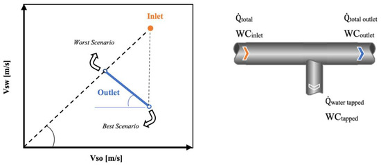
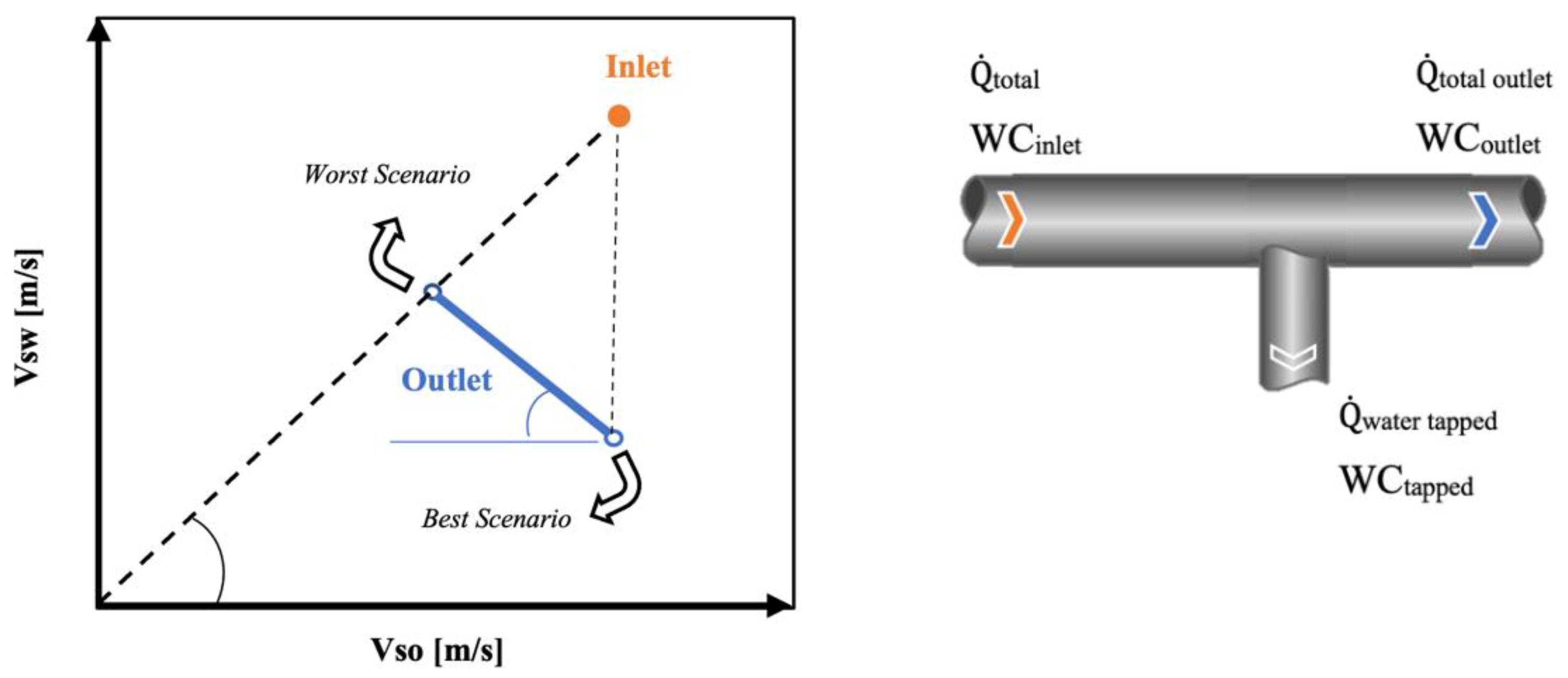
Consider an x-y scatter plot where the x axis represents the oil superficial velocity (Vso), and the y axis represents the water superficial velocity (Vsw). If a specific combination of oil and water flow rates approaching a tapping point is given (, ) and the pipe diameter is known, it is possible to pinpoint a tapping site on the plot (Point 1 in Figure 21, Vso1, Vsw1).
Figure 21.
Separation Triangle: representation of all possible separation efficiencies for a tapped flow rate in a superficial velocity plot [5].
The water cut in the drained stream could be anywhere from 100 percent (best scenario) to the stream’s water cut (WCinlet, worst scenario). Considering these two limit scenarios, stream 2 (downstream the tapping point) could fall on several locations over the blue line indicated in Figure 21. In terms of separation, it is best if it falls as close as possible to 2. Figure 22 shows a drainage potential curve measured for liquid rate of 580 L/min, WCinlet of 85% and for several tapped liquid rates.
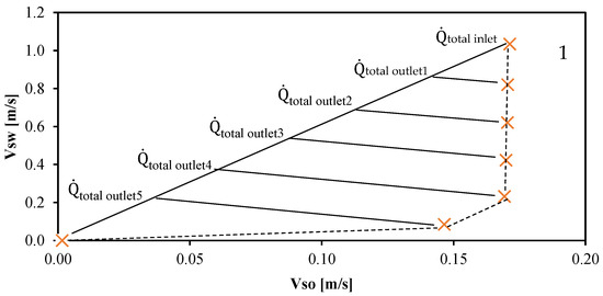
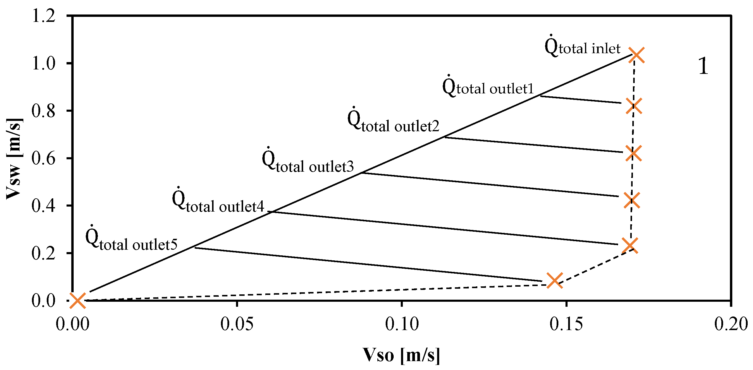
Figure 22.
Drainage potential curve for total flow rate 580 L/min and WCinlet 85%. [5].
5. Conclusions
Experimental drainage potential curves show a better separation performance (i.e., it is possible to extract high amounts of clean water) for low flow rates and high inlet water cuts. However, for most cases studied, it is possible to drain a significant fraction of the total inlet water without dragging significant amounts of oil through the tapping point.
Experimental drainage potential curves for the spiked and unspiked crude were similar for almost all cases, except for cases with low water cut and oil-dominated regimes. The separation performance with the spiked crude is worse than with the spiked crude. The drainage potential curves generated by numerical models compare well with the experimental curves. Satisfactory agreement is seen from this comparison. It is recommended to develop a more advanced numerical model that considers layers with different velocities or velocity profiles that tend to zero when approaching the pipe wall.
Author Contributions
Conceptualization, M.S.; methodology, S.H., M.S. and H.A.; software, S.H.; validation, H.A.; formal analysis, H.A. and S.H.; investigation, H.A. and S.H.; data curation, S.H. and H.A.; writing—original draft preparation, H.A.; writing—review and editing, M.S.; visualization, S.H.; supervision, M.S.; project administration, H.A.; funding acquisition, M.S. All authors have read and agreed to the published version of the manuscript.
Funding
This work was done as a part of SUBPRO, a research-based innovation center for subsea production and processing with project number 237893. The Department of Geoscience and Petroleum, NTNU, the Research Council of Norway, and key industry partners all contributed financially to SUBPRO, which the authors gladly acknowledge.
Institutional Review Board Statement
Not applicable.
Informed Consent Statement
Not applicable.
Data Availability Statement
Not applicable.
Acknowledgments
The authors thank the technical support of Sintef Multiphase Flow Lab in Tiller who gave us the opportunity to work with the mini-loop setup. The authors also acknowledge senior engineer, Noralf Vedvik, for his valuable support.
Conflicts of Interest
The authors declare no conflict of interest.
Nomenclature
| A | Cross section area [m2] | h | Height |
| D | Pipe diameter [m] | r | Radius [m] |
| Do/w | Dispersion of oil in water | t | Time [s] |
| Dw/o | Dispersion of water in oil | w | Width [m] |
| O | Oil | α | Volume fraction [-] |
| OiW | Oil in water emuslion | ||
| Q | Flow rate [L/min] | Subscript | |
| W | Water | in | Initial separation |
| WiO | Water in oil emulsion | o | Oil |
| WC | Water cut [%] | s | Superficial |
| WT | Tapping point efficiency [%] | sep | Complete separation |
| V | Velocity [m/s] | w | Water |
| VT | Control valve | y | Measured coordinate from the pipe bottom |
Appendix A. Characterization of Different Flow Pattern in Liquid-Liquid Flow Steam in Pipe
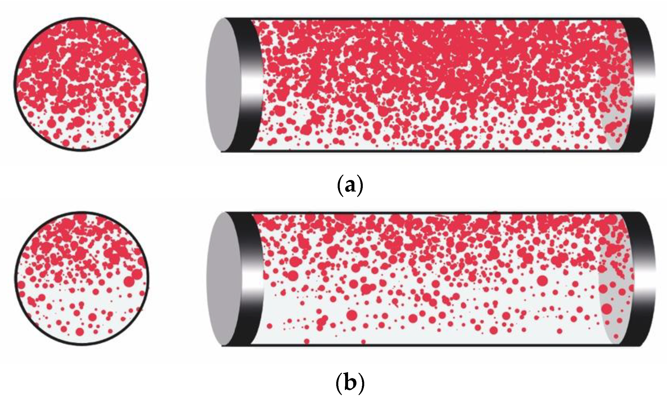
Oil dispersion in water: [Do/w]. High water superficial velocities and low to medium oil superficial velocities (e.g., 0.4 m/s) produce this flow configuration. The oil is split into little droplets by the shear forces and spread throughout the pipe’s cross section. The volume and size of the droplets might vary greatly depending on the fluid flows. As would be predicted for single-phase flow, the mixture velocity profile is parabolic and approximately centered within the pipe axis [17].
Figure A1.
Dispersion of oil in water [Do/w]. (a) High oil fraction, (b) low oil fraction.
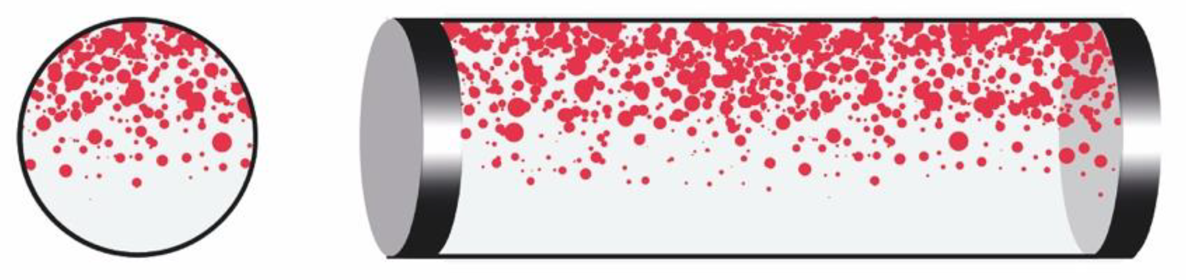
Dispersion of oil in water and water: [Do/w & W]. When the amount of water in the mixture is reduced (from Do/w), the turbulent forces in the mixture are reduced, allowing oil droplets to coalescence and grow in size. The distribution of the oil droplets is controlled by buoyancy forces, which push them to the top of the pipe, resulting in a clear (or almost transparent) water layer at the bottom [17].
Figure A2.
Dispersion of oil in water and water. [Do/w & W].
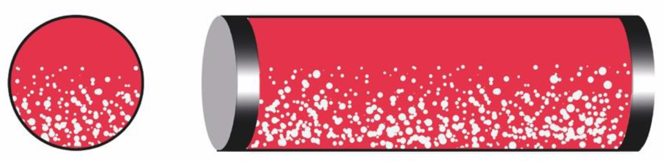
Oil and dispersion of water in oil: [O & Dw/o]. This structure is divided into two dominated layers of oil and water. Oil makes up the majority of the pipe’s upper portion. The pipe’s lower portion has a dual dispersion. Over a dispersion of oil in water, a dispersion of water in oil is noticed. This dual dispersion appears as a foam-like layer due to the high amount of turbulence [17].
Figure A3.
Oil and dispersion of water in oil. [O & Dw/o].
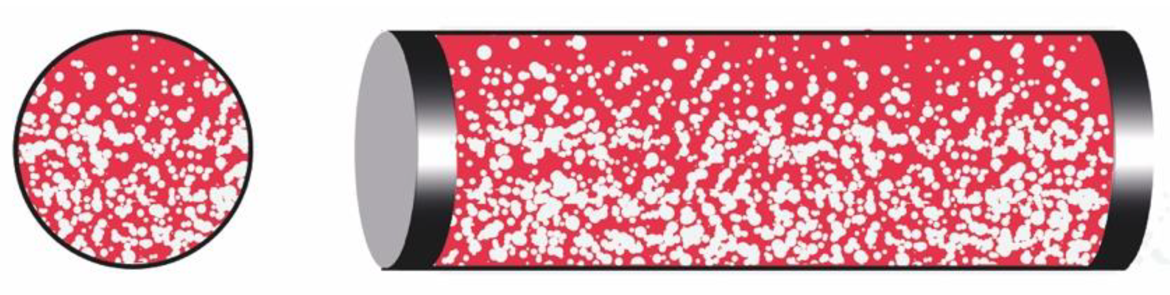
Dispersion of water in oil: [Dw/o]. The only flow configuration in which oil is the continuous phase across the pipe cross section is this one. Even though water is diffused in oil, it is concentrated at the bottom of the pipe in a foam-like structure similar to the one described above [17].
Figure A4.
Dispersion of water in oil. [Dw/o].
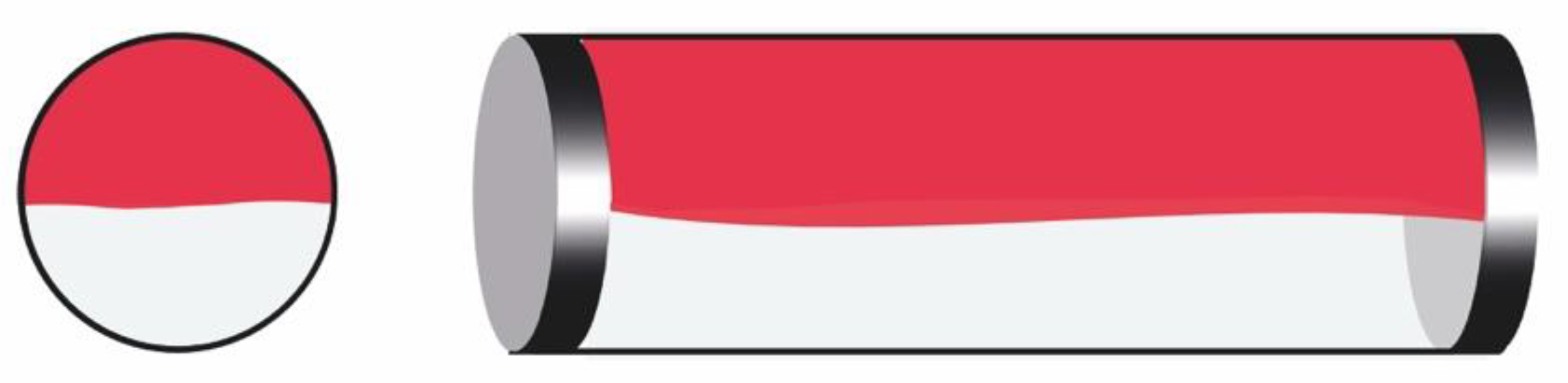
Stratified flow of water and oil: [O & W]. This flow configuration consists of two dominated, stratified and clear layers of water and oil without the presence of a noticeable dispersed/emulsion layer between the oil and water layers [17].
Figure A5.
Stratified flow of water and oil. [O & W].
Appendix B. Simplified Analytical Model to Compute Drainage Potential Curves of a Single Tapping Point in a Pipe Separator
The numerical model was built using the commercial software MatLab®.
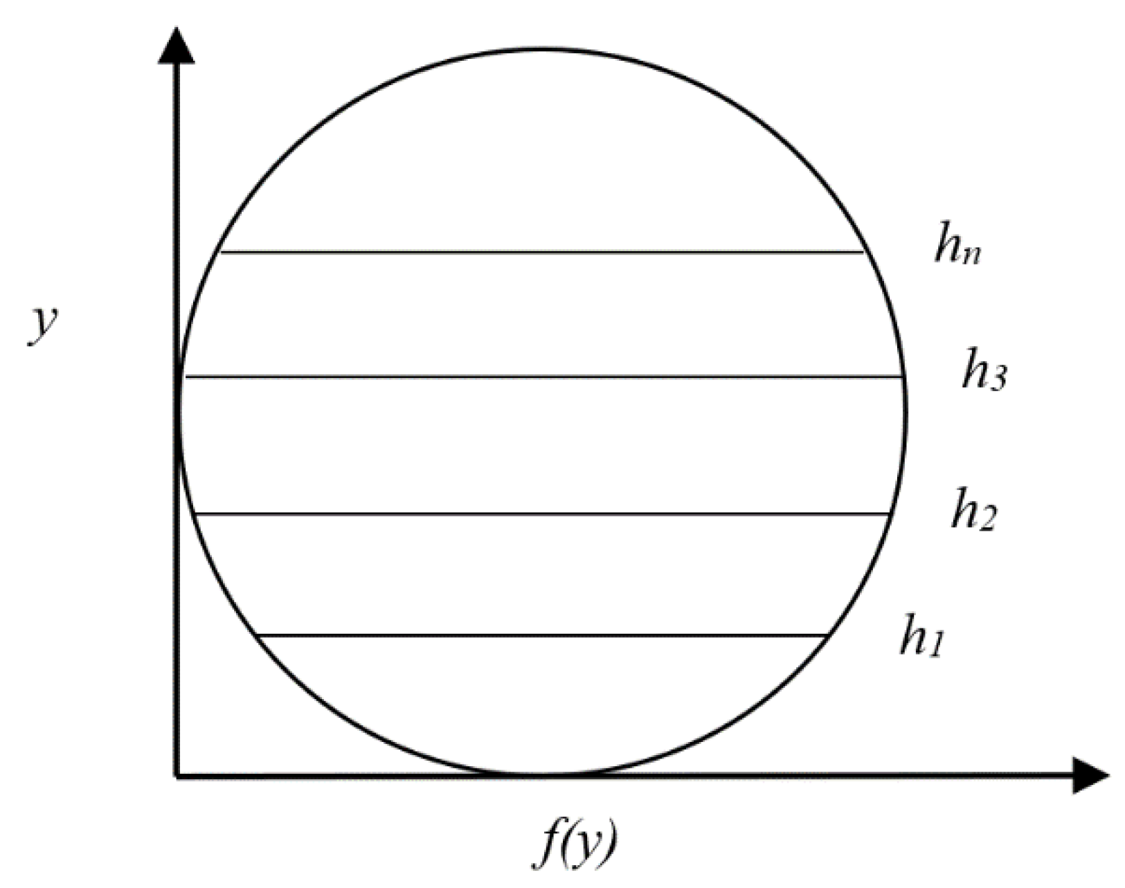
Figure A6.
Pipe section with fluid split along y = h.
Appendix B.1. Assumptions
- The fluid velocity in the pipe cross section is uniform and equal to the mixture velocity:
- There is no slippage between the fluids.
- The pipe has a circular cross section.
Appendix B.2. Drainage Potential Curve Model
The pipe cross section was split into horizontal slabs, as shown in Figure A6.
y is a coordinate measured from the pipe bottom. The area (A) of the cross section can be computed with the integral presented in Equation (A2).
where the pipe width at coordinate y is W(y). The WC of the mixture stream is:
Because there is no slip between fluids, the water cut of the mixture stream can also be calculated by integrating the water volume fraction along the pipe cross section.
It is assumed that tapping will drain part of the pipe cross section from the bottom of the pipe to a height h (with a horizontal interphase). The value of the flow rate tapped will define a height “h” drained. Therefore, the water cut of the tapped stream is
The total liquid drained is:
and Equation (A7), the total water drained.
In Equation (A8), the water drained was represented as a proportion of total water.
B.3. Width Function
The width w of a pipe segment was expressed as a function of y by using the following relationships:
For the lower half of the pipe,
For the centerline of the pipe,
For the upper half of the pipe,
Appendix B.4. Numerical Procedure to Determine the Distribution of Water Volume Fraction along the Vertical Axis
In the numerical solving process, two parameters were employed:
- The approximate pipe area was compared to the pipe’s geometrically determined cross sectional area, as stated in Equation (A15).
- 2.
- The inlet WC was estimated using Equation (A18) and compared against input WC input.
The Bisection Method described by Mathews et al., (2004) was used to determine the point of interface, i.e., WC 50%, that yielded an acceptable degree of error in the distribution obtained, as shown in Equation (A19) [23]. A relative inaccuracy of less than 1% was determined as the acceptable level of error. The pipe’s discretization was enhanced if relative errors in Equations (A17) and (A20), were greater than 1%
References
- Bradley, H.B. Petroleum Engineering Handbook; Society of Petroleum Engineers: Richardson, TX, USA, 1987. [Google Scholar]
- Skjefstad, H.S.; Stanko, M. Experimental performance evaluation and design optimization of a horizontal multi-pipe separator for subsea oil-water bulk separation. J. Pet. Sci. Eng. 2019, 176, 203–219. [Google Scholar] [CrossRef] [Scilit]
- Stanko, M. 2021. Available online: http://www.ipt.ntnu.no/~stanko/Resources.html (accessed on 1 August 2020).
- Mogseth, G. Functional verification of the worlds first full field subsea separation system-TIORA. In Proceedings of the Offshore Technology Conference, Houston, TX, USA, 5–8 May 2008. [Google Scholar]
- Stanko, M.; Golan, M. Simplified Hydraulic Design Methodology for a Subsea Inline Oil-Water Pipe Separator. In Proceedings of the OTC Brasil, Rio de Janeiro, Brazil, 27–29 October 2015. [Google Scholar]
- da Silva, F.S.; de Oliveira, D.A.; Moraes, C.A.C.; Marins, P.M. Subsea versus topside processing-conventional and new technologies. In Proceedings of the OTC Brasil, Rio de Janeiro, Brazil, 24–26 October 2013. [Google Scholar]
- Orlowski, R.; Euphemio, M.L.L.; Euphemio, M.L.; Andrade, C.A.; Guedes, F.; da Silva, L.C.T.; Pestana, R.G.; de Cerqueira, G.; Lourenço, I.; Pivari, A.; et al. Marlim 3 phase subsea separation system-challenges and solutions for the subsea separation station to cope with process requirements. In Proceedings of the Offshore Technology Conference, Houston, TX, USA, 30 April–3 May 2012. [Google Scholar]
- Abili, N.; Udofot, O.; Kara, F. Subsea Processing: A holistic approach to Marginal Field developments. In Proceedings of the Offshore Technology Conference, Houston, TX, USA, 30 April–3 May 2012. [Google Scholar]
- Pereyra, E.; Mohan, R.S.; Shoham, O. A simplified mechanistic model for an oil/water horizontal pipe separator. Oil Gas Facil. 2013, 2, 40–46. [Google Scholar] [CrossRef] [Scilit]
- SUBPRO. Annual Report 2018; Norwegian University of Science and Technology (NTNU): Trondheim, Norway, 2019; Available online: http://folk.ntnu.no/skoge/subpro-annual-reports/SUBPRO%20Annual%20Report%202018-2019.pdf (accessed on 19 March 2019).
- Skjefstad, H.S.; Stanko, M. An experimental study of a novel parallel pipe separator design for subsea oil-water bulk separation. In Proceedings of the SPE Asia Pacific Oil and Gas Conference and Exhibition, Brisbane, Australia, 19 October 2018. [Google Scholar]
- Keleşoğlu, S.; Keleşoğlu, S.; Rodionova, G.; Pettersen, B.H.; Foss, M.; Sjöblom, J. Preparation and characterization of reference fluids to mimic flow properties of crude oil emulsions (w/o). J. Dispers. Sci. Technol. 2015, 36, 1458–1464. [Google Scholar] [CrossRef] [Scilit]
- Kelesoglu, S. Flow Behaviour of Water-in-North Sea Acidic Crude Oil Emulsions and Preparation of Synthetic Reference Acidic Oils and Their Emulsions. Doctoral Thesis, Norwegian University of Science and Technology (NTNU), Trondheim, Norway, 2010. Available online: https://ntnuopen.ntnu.no/ntnu-xmlui/handle/11250/248240 (accessed on 1 June 2010).
- Rodionova, G.; Sjöblom, J. Electrorheological Behavior of Crude Oil and Synthetic Reference Fluid Emulsions. J. Dispers. Sci. Technol. 2015, 36, 1388–1393. [Google Scholar] [CrossRef] [Scilit]
- Hovden, L.; Lawrence, C.; Wold, I. Use of FACE flow loop data for validation and improvement of flow simulations. J. Dispers. Sci. Technol. 2015, 36, 1452–1457. [Google Scholar] [CrossRef] [Scilit]
- Kelesoglu, S.; Sjöblom, J. Synthetic crude oil. WIPO Patent Pub. No. WO/2011/161116; Patent Application No. PCT/EP2011/060370. US Patent Publication No. US 20130212929 A, 2011. [Google Scholar]
- Rivera, R.M.; Golan, M.; Friedemann, J.D.; Bourgeois, B. Water separation from wellstream in inclined separation tube with distributed tapping. SPE Proj. Facil. Constr. 2008, 3, 1–11. [Google Scholar] [CrossRef] [Scilit]
- Skjefstad, H.S.; Dudek, M.; Øye, G.; Stanko, M. The effect of upstream inlet choking and surfactant addition on the performance of a novel parallel pipe oil–water separator. J. Pet. Sci. Eng. 2020, 189, 106971. [Google Scholar] [CrossRef] [Scilit]
- Elseth, G. An Experimental Study of Oil/Water Flow in Horizontal Pipes. Ph.D. Thesis, Norwegian University of Science and Technology (NTNU), Trondheim, Norway, 2001. [Google Scholar]
- Skjefstad, H.S. Development and Assessment of a Multi-Pipe Oil-Water Bulk Separator Concept for Subsea Applications. Ph.D. Thesis, Norwegian University of Science and Technology (NTNU), Trondheim, Norway, 2019. [Google Scholar]
- Trallero, J.; Sarica, C.; Brill, J. A study of oil/water flow patterns in horizontal pipes. SPE Prod. Facil. 1997, 12, 165–172. [Google Scholar] [CrossRef] [Scilit]
- Kokal, S. Crude Oil Emulsions: Everything You Wanted to Know But Were Afraid to Ask; Society of Petroleum Engineers: Richardson, TX, USA, 2008. [Google Scholar]
- Mathews, J.H.; Fink, K.D. Numerical Methods Using MATLAB; Pearson Prentice Hall: Upper Saddle River, NJ, USA, 2004; Volume 4. [Google Scholar]

Publisher’s Note: MDPI stays neutral with regard to jurisdictional claims in published maps and institutional affiliations. |
© 2022 by the authors. Licensee MDPI, Basel, Switzerland. This article is an open access article distributed under the terms and conditions of the Creative Commons Attribution (CC BY) license (https://creativecommons.org/licenses/by/4.0/).