


Abstract
The Discounted Cash Flow (DCF) methodology is widely regarded as one of the most theoretically well-established approaches to firm valuation. The most critical issue within this methodology is the reliable and well-grounded estimation of those cash flows, particularly the systematic incorporation of qualitative enterprise risks into future cash-flow projections. The objective of this study is to develop a systematic and standardized methodology for estimating risk-adjusted cash flows based on a set of parameters derived from the Internal Control System (ICS) of the firm under valuation, operationalized through a rating system focused on the qualitative dimensions of the company. The proposed framework systematically translates qualitative risk assessments into explicit adjustments of the economic drivers underlying projected cash flows, thereby establishing a structured link between Internal Control Systems (ICS), Enterprise Risk Management (ERM), and Discounted Cash Flow (DCF) valuation. The methodology is applied to a baseline financial scenario representing the central financial projection of the firm, which is subsequently adjusted for enterprise risks derived from the Internal Control System. Naturally, quantitative factors must also be considered; however, this issue has already been extensively examined in the literature and is firmly established in corporate finance textbooks. The contribution of this paper lies in providing the academic and professional communities with a systematic framework designed to improve the transparency, consistency, and traceability of firm valuation while supporting a more structured incorporation of qualitative risk factors into projected cash flows. The proposed framework is methodological in nature and is intended to provide a conceptual foundation for future empirical calibration and validation using real-world corporate data.
1. Introduction
Firm valuation constitutes one of the central fields of corporate finance from both academic and professional perspectives. Within this field, there is broad consensus regarding the theoretical superiority of the Free Cash Flow Discounted Model (DCF) as a tool for estimating the intrinsic value of a company, since it is based on the firm’s future capacity to generate economic resources. From a broader investment and business valuation perspective, the assessment of expected future cash flows and the risks associated with their realization constitutes a fundamental component of investment appraisal and corporate valuation (Hering, 2021, 2022). Nevertheless, it is also generally accepted that every valuation process inevitably incorporates certain degrees of subjectivity, primarily derived from the need to formulate estimates concerning future variables.
Such subjectivity becomes particularly evident in the projection of the free cash flows to be discounted. Since these are prospective estimates, there is an inherent risk of deviation between projected values and those ultimately realized. From a technical standpoint, these cash flows may be decomposed into two differentiated layers: on the one hand, the free cash flows explicitly projected over a time horizon considered reasonable; on the other hand, the value corresponding to the period beyond such horizon, extending into perpetuity and generally estimated through a constant growth rate “g” applied to the free cash flow from the end of the explicit forecast period onward.
The management of the risk associated with these estimates has traditionally been addressed through various approaches. Among the most common are adjustments to the discount rate in order to reflect the assumed level of risk, the estimation of risk-adjusted cash flows, and the construction of alternative future cash flow scenarios accompanied by probabilities that allow the calculation of an expected value and the performance of dispersion analyses. Academic literature has devoted considerable attention to the study of adjustment mechanisms in the discount rate; however, the analysis relating to the rigorous and well-grounded estimation of the free cash flows themselves has received comparatively less attention (Damodaran, 2007; Brealey et al., 2020). In particular, existing valuation approaches provide only limited guidance on how qualitative enterprise risks identified through Internal Control Systems (ICS) can be systematically translated into projected cash flows while preserving transparency, consistency, and traceability throughout the valuation process.
Within this context, two principal approaches may be identified for addressing cash flow estimation under uncertainty: (i) the construction of multiple future scenarios associated with alternative assumptions and probabilities; and (ii) the estimation of a single baseline cash flow path representing the central financial projection, which may subsequently be adjusted for explicitly identified enterprise risks (Copeland et al., 2000; Damodaran, 2012). The present study follows the latter approach. More specifically, the initial cash-flow projections used in this study represent the base-case, or most likely, financial scenario and should not be interpreted as an optimistic scenario. The proposed methodology adjusts the cash flows of this base-case scenario according to internal enterprise-risk factors identified and assessed through the Internal Control System (ICS). The resulting cash flows therefore represent internally risk-adjusted base-case cash flows. Accordingly, the methodological contribution of the present study focuses specifically on the systematic estimation of these internal-risk adjustments rather than on the construction of alternative financial scenarios.
Although the latter approach does not immediately facilitate contingency analysis under adverse scenarios, it offers significant advantages: it allows the structured definition of a base-case path of future free cash flows and provides a structured basis for the subsequent construction of probabilistic scenarios with an acceptable degree of rigor aimed at the design of contingency plans.
Based on these considerations, the objective of this study is to develop a structured methodological framework that systematically integrates qualitative risk assessments derived from the Internal Control System (ICS) into Discounted Cash Flow (DCF) valuation by translating those assessments into explicit risk-adjusted cash-flow projections. The proposed methodology establishes a structured link between Internal Control Systems (ICS), Enterprise Risk Management (ERM), and corporate valuation through a rating-based framework that connects qualitative risk assessments with the economic drivers underlying projected cash flows. To support this proposal, it is necessary to critically examine the current state of the literature, identify its principal contributions, and delimit the conceptual and methodological gaps that still remain.
The contribution of this study is threefold. First, it proposes a structured methodology for translating qualitative risk assessments into explicit cash-flow adjustments. Second, it establishes a systematic analytical link between Internal Control Systems, Enterprise Risk Management, and Discounted Cash Flow valuation. Third, it introduces a transparent and traceable rating-based framework designed to support a more consistent incorporation of qualitative enterprise risks into firm valuation while avoiding the double counting of overlapping risk effects.
The article is structured as follows. Following this introduction, Section 2 presents a literature review and identifies the research gap motivating the study. Section 3 develops the methodological foundations and operational structure of the proposed model. Section 4 presents the conclusions, limitations, and future research directions. An illustrative application of the methodology using a fictional company and projected financial statements is provided in Appendix A, while the supporting financial projections are reported in Appendix B.
This study is methodological in nature and does not seek to empirically validate the proposed framework. The illustrative application presented later serves exclusively to demonstrate the operational implementation of the methodology.
Future empirical research will be required to calibrate, validate, and assess the predictive performance of the proposed framework using real-world corporate data.
2. Literature Review and Identification of the Research Gap
The literature on internal control systems and risk management has experienced significant development in recent decades. In this regard, the conceptual framework promoted by the Committee of Sponsoring Organizations of the Treadway Commission (COSO) stands out, as its reports have provided the foundation for the structuring of internal control systems and their subsequent integration into Enterprise Risk Management (ERM) models (Committee of Sponsoring Organizations of the Treadway Commission [COSO], 2013, 2017; McKay, 2013; Prewett & Terry, 2018; Nielsen & Pontoppidan, 2020; Hadi et al., 2025; Huang, 2026). More recently, research has further emphasized that effective Internal Control Systems contribute not only to regulatory compliance but also to organizational resilience, corporate governance, strategic decision-making, and long-term firm value (Chen et al., 2020; Yun, 2023; Guo et al., 2024; Indriastuti et al., 2025). These developments have provided systematic frameworks for the identification, classification, and management of risks across different business sectors.
Complementarily, numerous studies have examined the role of internal control systems in the construction of risk taxonomies (Hopkin, 2018; Bondarenko et al., 2021) and in the improvement of risk management and monitoring processes (Turgaeva, 2024; Spira & Page, 2003; Shin & Park, 2017; Mohammed et al., 2021; Peng & Jin, 2025). However, the literature examining the contribution of such systems to the quantitative valuation of identified risks—and, particularly, their integration into scoring models capable of estimating the financial impact of qualitative factors on cash flows—remains significantly more limited. The scarce contributions in this area focus primarily on the need to incorporate such factors into DCF models (Kazlauskienė & Christauskas, 2007; Razali et al., 2022; Meitner & Streitferdt, 2014), without developing sufficiently structured operational frameworks for their systematic quantification. Although recent studies increasingly acknowledge the relevance of enterprise risk management for value creation, they rarely provide operational methodologies capable of translating Internal Control System assessments into explicit cash-flow adjustments (Yun, 2023; Guo et al., 2024).
Likewise, the systematic analysis of qualitative risk factors directly affecting cash flows has received limited attention in academic literature. Variables such as market conditions, operational efficiency, and management quality—among others—exert a decisive influence on the stability and predictability of future cash flows and are therefore critical for the accuracy of cash flow projections and, consequently, for comprehensive firm valuation (Oh et al., 2020). In this regard, financial decision-making requires the explicit assessment of the impact of risk, credit rating, and firm value, given their combined effect on the estimation of economic value (Blum et al., 2018). Recent contributions further suggest that qualitative governance characteristics and enterprise resilience increasingly influence investors’ valuation assessments, reinforcing the need for structured methodologies capable of incorporating these dimensions into business valuation (Khandelwal et al., 2023; Li et al., 2025; Wibowo et al., 2025).
Moreover, the incorporation of risk into Discounted Cash Flow (DCF) models through adjustments applied to cash flows under certainty conditions (certainty equivalent method)—which consist of directly adjusting the expected value of future cash flows, thereby reducing the valuation base—has been extensively analyzed in the literature. These approaches have been thoroughly examined both from the perspective of their methodological characteristics and limitations, as well as regarding possible criteria for improvement and refinement (Kudla, 1980; Brick & Weaver, 1984; Goehr & Kupke, 2003; Damodaran, 2007). More broadly, three principal approaches currently dominate the valuation literature for incorporating uncertainty into DCF models: (i) adjustments to the discount rate (risk-adjusted discount rate approach), (ii) certainty-equivalent cash-flow adjustments, and (iii) scenario-based valuation techniques. While these approaches differ in their implementation, all ultimately rely on analyst judgement to incorporate qualitative sources of operational risk and do not provide a structured mechanism linking Internal Control System assessments directly to projected cash flows.
From an academic perspective, one of the principal limitations of the risk-adjustment method lies in its inability to explicitly quantify qualitative factors affecting corporate risk, such as management quality, regulatory risk, institutional stability, or corporate reputation. The method assumes that all uncertainty can be incorporated through certainty-equivalent coefficients applied to expected cash flows, which reflect the decision-maker’s risk aversion. However, the determination of such coefficients generally depends on subjective judgments that are difficult to validate empirically, particularly when risks cannot be easily translated into probabilistic distributions (Brealey et al., 2020). Consequently, the method tends to oversimplify the multidimensional nature of risk by reducing it to a single numerical adjustment that may conceal relevant sources of uncertainty not strictly financial in nature. Similarly, risk-adjusted discount rate approaches aggregate heterogeneous sources of operational, strategic, and governance risk into a single discount-rate adjustment, thereby limiting transparency regarding the specific drivers of enterprise risk. Scenario analysis partially addresses this limitation by considering alternative future outcomes; however, its application becomes increasingly complex as the number of relevant qualitative risk factors grows.
Furthermore, the literature indicates that the absence of a formal structure for incorporating qualitative risk factors generates consistency and comparability problems among projects evaluated under the certainty-equivalent approach. In this regard, Damodaran (2012) highlights that, in practice, analysts often end up adjusting coefficients on an ad hoc basis in order to reflect qualitative perceptions, thereby weakening the transparency and reproducibility of the valuation process. Moreover, existing valuation approaches provide only limited guidance regarding the treatment of interdependent operational risks affecting identical economic variables. Consequently, overlapping risk effects may inadvertently be incorporated more than once into projected cash flows, increasing the likelihood of double counting.
Therefore, the existing academic literature presents a significant gap regarding the development and application of scoring models for qualitative risk factors grounded in Internal Control Systems. In particular, there is limited integration of such models with algorithms capable of quantifying the impact of risk events on future cash flows. This methodological deficiency restricts the systematic incorporation of qualitative risk factors into business valuation processes, especially those based on the Discounted Cash Flow (DCF) approach. Consequently, there is a clear need to develop analytical frameworks capable of translating the qualitative factors identified by internal control systems into quantifiable metrics that can be operationally integrated into cash flow projections. More specifically, no integrated methodological framework has yet been proposed that systematically combines Internal Control Systems, Enterprise Risk Management, qualitative risk scoring, and Discounted Cash Flow valuation while simultaneously addressing the consolidation of overlapping operational risks and preventing double counting.
The present study seeks to contribute to overcoming this gap through the proposal of a methodological model aimed at constructing a baseline free cash flow path explicitly adjusted for the financial impact of qualitative risk factors structured through the firm’s internal control system. Unlike existing approaches, the proposed framework integrates Internal Control Systems, Enterprise Risk Management, and Discounted Cash Flow valuation within a unified methodological structure. The study contributes by (i) providing a standardized rating-based methodology for translating qualitative Internal Control System assessments into explicit risk-adjusted cash-flow projections, (ii) introducing a structured consolidation procedure that prevents double counting of overlapping risk effects, (iii) improving the transparency, consistency, and traceability of valuation decisions, and (iv) providing a methodological foundation that can subsequently be calibrated and empirically validated using real company data. The research gap identified in this section directly motivates the methodological framework developed in Section 3.
3. Model
3.1. Methodological Foundations
Based on the gap identified in the literature, the present study proposes a methodological approach aimed at improving the transparency, consistency, and structured incorporation of enterprise risk into cash flow projections through the explicit incorporation of business risk identified by internal corporate information systems.
The objective of the proposed methodology is not to replace conventional Discounted Cash Flow (DCF) valuation, but rather to complement existing valuation techniques by providing a structured procedure through which qualitative enterprise risks identified by Internal Control Systems (ICS) can be translated into explicit cash-flow adjustments. Accordingly, the framework should be understood as an extension of traditional DCF valuation rather than as an alternative valuation model.
The proposed framework does not modify the conventional estimation of the Weighted Average Cost of Capital (WACC). Enterprise risks explicitly quantified through the methodology are incorporated through adjustments to the economic drivers of projected cash flows rather than through an additional discretionary risk premium in the discount rate. Accordingly, risks already incorporated through the risk-adjusted cash-flow mechanism should not be reflected again through ad hoc adjustments to WACC. Market-based systematic risk and financing-related determinants of the discount rate remain treated according to conventional corporate-finance principles. This separation between cash-flow risk adjustments and discount-rate determination is intended to reduce the potential for double counting between numerator- and denominator-based risk adjustments.
The model is grounded on a key premise: business risks do not directly affect financial aggregates such as EBIT or Free Cash Flow (Damodaran, 2007; Brealey et al., 2020), but rather the underlying economic variables that are subsequently reflected in such aggregates (Razali et al., 2022). Consequently, adjustments derived from risk assessment should be applied to these specific economic drivers rather than to aggregated financial magnitudes.
This premise is consistent with the causal logic of corporate finance. Operational risks first influence the underlying economic drivers of value creation—including revenues, operating costs, inventories, receivables, production efficiency and capital expenditures—which subsequently determine accounting aggregates such as EBIT, Operating Cash Flow and ultimately Free Cash Flow. The proposed methodology therefore applies risk adjustments at the level where risks economically originate rather than where they are merely reflected in financial statements.
This approach is consistent with the business valuation literature, which emphasizes the analysis of operational value drivers as the basis for rigorous estimation (Rappaport, 1998; Damodaran, 2007; Koller et al., 2020).
From a methodological perspective, this approach presents four main contributions. First, it improves the economic consistency of the model by linking each risk to the variable that actually determines its financial impact (Kazlauskienė & Christauskas, 2007). Second, it facilitates the identification and elimination of duplications, thereby avoiding the problem of double counting when different risks simultaneously affect the same economic variable (Shin & Park, 2017). Third, it proposes a scoring system that allows risk to be quantified through normalized numerical metrics. Fourth, the methodology introduces a structured consolidation mechanism that explicitly analyses interdependencies between operational risks, thereby reducing the likelihood of double counting when different business processes affect the same economic variable.
Furthermore, the proposal is aligned with the Enterprise Risk Management (ERM) literature, which highlights the need to integrate risk analysis into corporate decision-making processes and internal control systems (Hoyt & Liebenberg, 2011). In this context, the model is structured as a systematic procedure that translates qualitative risk assessment into nominal adjustments applied to specific economic variables, ensuring causal traceability between the identified risk, its transmission channel, and its final financial impact on cash flow.
Unlike traditional certainty-equivalent approaches, which generally rely on subjective certainty-equivalent coefficients to adjust projected cash flows, the proposed methodology derives adjustments from documented enterprise-risk assessments performed within the Internal Control System. Consequently, every adjustment incorporated into projected cash flows can be traced back to a specific operational process, affected economic variable and documented risk assessment, thereby improving transparency, reproducibility and auditability.
The previous considerations highlight the need for an analytical framework capable of systematically translating business risk events into quantifiable financial impacts (Andrén et al., 2005). To this end, it is necessary to formalize the mechanism through which risks identified within organizational processes are transmitted to the economic drivers of cash flow.
The starting point of the analysis is the expression used to estimate firm value at a given moment (V0) through the discounting of free cash flows:
where:
- = weighted average cost of capital
- FCFfRA = risk-adjusted Free Cash Flow
- = terminal value
The terminal value is calculated from the last estimated FCF considering a growth rate “g” and using risk-adjusted cash flows:
The proposed methodology focuses on the estimation of the numerator of the first term of the expression determining V0, namely the risk-adjusted Free Cash Flow, which is obtained by subtracting the risk adjustments (VRt) from the baseline cash flow:
where:
- = projected Free Cash Flow without explicit risk adjustment.
- = aggregate economic value of business risk in period t.
The model proposes that such economic value of risk can be estimated as the sum of the nominal adjustments associated with each affected economic variable:
where:
- = economic base exposed to risk;
- = risk materialization coefficient;
- = residual factor derived from the risk scoring system;
- = number of affected economic variables.
Accordingly, the central formulation of the model is:
The formulation should be interpreted as a conceptual methodological framework rather than as a calibrated empirical model. Its purpose is to define the analytical structure through which enterprise risks may be systematically translated into cash-flow adjustments. The empirical estimation and statistical calibration of the proposed parameters constitute a subsequent stage of research discussed in Section 4.3.
The economic exposure base , the materialization coefficient , and the residual factor constitute the three fundamental components through which enterprise risk is translated into nominal financial adjustments. Their operational determination is developed in Phases 4 to 6 of the methodological procedure presented in Section 3.2.
The materialization coefficient is conceptually defined as the interaction between the expected frequency of the risk event and the absorption capacity provided by the Internal Control System and other relevant operational and strategic mitigation measures:
where:
- represents the expected probability of occurrence of the risk event;
- represents the mitigation and absorption capacity provided by the Internal Control System and other relevant operational and strategic mitigation measures.
The multiplicative specification reflects the assumption that the expected economic impact of a risk depends simultaneously on its probability of occurrence and on the organization’s capacity to absorb or mitigate its consequences. If either component approaches zero, the expected economic impact is proportionally reduced. Consequently, the interaction between both dimensions provides a more economically meaningful representation of expected risk materialization than an additive specification.
It should be emphasized that a lower materialization coefficient does not indicate lower enterprise risk. Rather, it reflects that a smaller proportion of the economic exposure is expected to remain after considering the combined effect of occurrence probability and the mitigation capacity provided by the Internal Control System. Consequently, the materialization coefficient should be interpreted as a parameter of expected materialization rather than as a direct measure of overall risk severity.
Likewise, the conditional severity factor is obtained from a separate assessment of the economic severity of the risk conditional on materialization:
where:
- ScoreSevI is the overall risk score assigned to risk i;
- represents the calibration function transforming the conditional severity score into an economic severity factor.
The conditional severity factor captures the magnitude of the economic consequences conditional on risk materialization. Consequently, the materialization coefficient (CM) and the conditional severity factor (FR) describe complementary rather than overlapping dimensions of enterprise risk. While CM estimates the proportion of the exposure expected to materialize after considering occurrence probability and mitigation effectiveness, FR reflects the economic severity of the consequences conditional on such materialization. Therefore, the simultaneous use of both parameters does not generate double counting provided that the underlying scoring dimensions remain analytically separate.
Thus, the expression
represents the expected nominal adjustment associated with each economic variable affected by enterprise risks.
In practical applications, the overall process scores are expected to be assigned through structured governance procedures involving multidisciplinary assessment teams comprising Internal Audit, Risk Management, Operational Management and, where appropriate, external valuation specialists. The objective is to reduce individual analyst subjectivity by relying on documented collective assessments supported by the organization’s Internal Control System.
The proposed formulation is based on four fundamental methodological principles:
- The principle of economic causality, according to which adjustments must be applied to underlying economic variables rather than directly to aggregated financial items.
- The principle of risk-impact traceability, whereby each component of the nominal adjustment represents the expected economic effect of a risk identified within the internal control system.
- The principle of consolidation without double counting, which requires the prior elimination of interdependencies between risks and processes before their aggregation into , thereby ensuring that the adjustments do not include redundant economic effects on the same variable.
- Methodological transparency.
The principle of methodological transparency, according to which every adjustment incorporated into projected cash flows must remain fully traceable to documented risk assessments, affected economic variables and underlying business processes.
On this basis, the model requires an operational procedure capable of identifying, estimating, and consolidating its different components from the business risk assessment. The following section develops this procedure sequentially.
Accordingly, Section 3.2 operationalizes these theoretical principles through a structured nine-phase methodology that translates enterprise-risk assessments into risk-adjusted Free Cash Flow while preserving economic causality, methodological transparency, traceability and consistency throughout the valuation process.
3.2. Operational Development of the Model
The operational implementation of the model is structured into nine sequential phases that translate enterprise risk assessments into risk-adjusted cash flows. The procedure identifies affected economic variables, quantifies the economic exposure, estimates the expected impact through the materialization coefficient and residual factor, and consolidates the resulting adjustments to determine the aggregate value of risk and the corresponding risk-adjusted cash flow.
The procedure is designed to be implemented through a documented and multidisciplinary assessment process. In practical applications, risk identification, scoring, parameter assignment, and validation should involve representatives from Risk Management, Internal Audit, the relevant process owners, Finance, and, where appropriate, external valuation specialists. Each assessment should be supported by documented evidence, including risk registers, control-testing results, historical loss events, key risk indicators, audit findings, and financial or operational data. This governance structure is intended to improve consistency between evaluators, transparency, reproducibility, and auditability.
The parameter ranges presented below constitute provisional methodological calibration choices for the illustrative application rather than empirically estimated, externally validated, or universally applicable thresholds. Their purpose is to demonstrate the operational logic of the methodology and to provide a basis for subsequent empirical calibration using real-world data.
Table 1 presents an integrated overview of the methodological procedure. For each phase, the table relates the inputs derived from the risk assessment system, the analytical treatment applied, the specific model component determined at each stage, and the methodological result obtained. This synthesis allows a structured visualization of how the model translates business risk into traceable nominal financial adjustments.
Table 1.
Integrated Methodological Structure of the Model.
For practical implementation, each phase should additionally document the evidence used, the responsible evaluator, the validating function, and any assumptions introduced. This documentation enables every adjustment to be traced from the original risk assessment to its final impact on projected cash flow.
Figure 1 summarizes the causal structure of the model linking enterprise risk assessment, affected economic variables, nominal adjustments, and risk-adjusted cash flow.
Figure 1.
Conceptual Architecture of the Risk-Adjusted Cash Flow Model. Source: Authors’ own elaboration.
The revised figure should visually distinguish four analytical blocks: (i) risk identification and causal mapping; (ii) exposure and parameter estimation; (iii) interdependency consolidation; and (iv) integration into the DCF valuation. It should also display the relationships among and FCFRA.
3.2.1. Phase 1: Identification of Economic Variables Subject to Impact and Their Reflection in Cash Flow
Phase 1 identifies the economic variables affected by enterprise risk and their transmission channels to cash flow. Consistent with the valuation literature, risks are assumed to affect underlying economic drivers rather than accounting aggregates such as EBIT or Free Cash Flow. Accordingly, the model focuses on variables such as material costs, inventories, operating margins, accounts receivable, and CAPEX, whose effects are subsequently reflected in operating income, working capital, or investment cash flow.
The current framework focuses specifically on downside enterprise risk, understood as the potential adverse deviation of economic drivers from the baseline cash-flow projection. Positive deviations and opportunity-related risks fall outside the present scope and may be incorporated in future extensions through symmetric or asymmetric upside-adjustment mechanisms.
To prevent double counting, the baseline cash-flow projection must be defined before the explicit incorporation of the risks quantified by the model. Risks already embedded in projected revenues, costs, margins, working-capital assumptions, or investment plans should not be adjusted a second time. The baseline should be interpreted as the central or reference financial scenario of the valuation and not as an optimistic scenario. The baseline therefore represents the financial projection before the explicit, documented risk adjustments introduced through the proposed framework.
The relevant structure of cash flow may be functionally decomposed into different economic and financial blocks. For consistency with conventional corporate-finance definitions, Free Cash Flow to the Firm may be expressed as follows:
where:
FCFt = EBITt (1 − Tt) + D&At − ΔNWCt − CAPEXt
- EBITt (1 − Tt) represents Net Operating Profit After Taxes;
- D&At represents depreciation and amortization;
- ΔNWCt represents the increase in net working capital; and
- CAPEXt represents capital expenditures.
This formulation avoids counting investment in working capital both as part of operating cash flow and as an additional investment cash-flow item.
This decomposition allows a distinction to be made between causal risk variables and derived financial aggregates, an aspect that is essential for rigorous quantification of the economic impact of risk. It is important to emphasize that EBIT does not constitute a cash flow position in itself, but rather an accounting aggregate reflecting the joint effect of underlying economic variables (margins, costs, inefficiencies). Financial literature warns that income aggregates may conceal the true exposure to risk if their operational determinants are not analyzed (Brealey et al., 2020; Razali et al., 2022).
Consequently, risk adjustments should not be applied directly to EBIT or Free Cash Flow, but rather to the economic variables that determine them. This approach preserves the economic causality of the model, ensures traceability between risk and financial impact, and facilitates the subsequent consolidation of impacts without double counting. The main characteristics and differences between these approaches are summarized in Table 2.
Table 2.
Economic Variables Affected and Their Financial Reflection.
The result of this phase is the construction of a map of economic variables subject to impact, which act as channels for the transmission of risk toward cash flow. This map constitutes the basis for the causal allocation of risks in Phase 2 and allows the correct consolidation of convergent impacts, the preservation of traceability between risk and financial effect, and the avoidance of double counting between processes, in line with the literature on the integration of risk management and internal control (Shin & Park, 2017; Spira & Page, 2003).
3.2.2. Phase 2: Identification of the Cash Flow Position Affected by Each Risk
Phase 2 assigns each identified risk to a specific economic variable and transmission channel. This mapping establishes the causal relationship between operational risk and financial impact, generating a risk–economic variable correspondence matrix that serves as the basis for subsequent quantification.
Each relationship should be supported by a documented causal rationale specifying:
- the originating business process;
- the relevant risk event and control deficiency;
- the mechanism through which the risk affects the business;
- the directly affected economic variable;
- the corresponding cash-flow component;
- the expected timing and duration of the impact; and
- the source of evidence supporting the relationship.
The resulting correspondence matrix should therefore contain, at a minimum, the risk event, process, control deficiency, transmission channel, economic variable, Free Cash Flow component, time horizon, and evidence source. The causal allocation should be validated jointly by the process owner and Finance or the valuation specialist to ensure economic plausibility.
3.2.3. Phase 3: Aggregation of Risks at the Process Level and Internal Netting
Phase 3 consolidates risks at the process level to avoid redundant estimates when multiple risks affect the same economic variable. This phase is limited to within-process deduplication. Risks belonging to the same process and representing the same causal event, control deficiency, or economic consequence are consolidated before monetary quantification. Cross-process dependencies and partial overlaps between different organizational processes are addressed exclusively in Phase 8.
Two criteria are applied:
- Complete equivalence: when two risks represent substantially the same causal event and economic effect, only one consolidated risk is retained.
- Distinct incremental contribution: when the risks affect the same variable but generate economically separable effects, both may be retained if their incremental contributions can be documented.
The result is a consolidated set of relevant risks by process and economic variable, prior to the determination of the monetary exposure base.
3.2.4. Phase 4: Definition of the Economic Exposure Base
Phase 4 determines the economic exposure base (BE), defined as the monetary amount effectively exposed to risk. Typical exposure bases include material costs, inventory balances, operating margins, and CAPEX.
The exposure base should represent the maximum economically relevant amount causally exposed to the specific risk, rather than automatically corresponding to the total accounting balance. Where only part of a balance or transaction population is affected, only that portion should be used as the exposure base.
The exposure base should be determined according to the following hierarchy:
- directly observable amounts specifically exposed to the risk;
- reconciled financial-statement balances;
- operational data converted into monetary values;
- historical-loss or incident-based estimates; and
- structured expert estimates when reliable quantitative data are unavailable.
For reproducibility, the source, reference date, measurement period, unit, financial-statement reconciliation, assumptions, and responsible validator should be documented.
3.2.5. Phase 5: Determination of the Materialization Coefficient (CM)
Once the economic exposure base has been identified, the next step consists of estimating the proportion of that exposure that may effectively materialize during the period under analysis. For this purpose, the model introduces the materialization coefficient (CM), which transforms potential exposure into expected economic impact.
The materialization coefficient is conceptually defined as:
where
- F_frequency represents the annual probability of occurrence of the risk and is derived from the scoring associated with the net probability of the risk, as evaluated in the risk control matrices;
- F_absorption reflects the residual proportion of the economic exposure expected to remain after considering the effectiveness of the Internal Control System (ICS) and existing operational and strategic mitigation measures. Consequently, higher values of Fabsorbtion indicate greater residual exposure after mitigation, whereas lower values reflect stronger mitigation capacity and lower residual exposure.
Accordingly, the coefficient captures two complementary dimensions of risk: the likelihood of occurrence and the organization’s capacity to mitigate its consequences. More precisely, CM represents the expected proportion of the economic exposure that remains economically relevant after jointly considering the probability of occurrence and the residual exposure after mitigation. Accordingly, the materialization coefficient provides a structured mechanism for translating qualitative Internal Control System assessments into an expected economic exposure while preserving the causal relationship between operational risk and projected cash flows. Accordingly, the materialization coefficient should not be interpreted as a standalone indicator of enterprise risk. Its economic interpretation is limited to the expected proportion of the exposure that is expected to materialize after considering both occurrence probability and mitigation effectiveness.
It should be noted that the materialization coefficient does not measure the overall intensity of risk. Rather, it represents the expected proportion of the economic exposure base that may materialize after considering both the probability of occurrence and the mitigating effect of the Internal Control System. The overall magnitude of the risk adjustment is determined jointly by the materialization coefficient and the residual factor introduced in Phase 6.
The materialization coefficient therefore reflects the expected proportion of the exposure likely to materialize, whereas the residual factor introduced in Phase 6 captures the conditional economic severity of the impact once materialization has occurred.
Higher frequencies and weaker mitigation capacities lead to higher materialization coefficients, whereas lower frequencies and stronger mitigation capacities lead to lower materialization coefficients.
For operational purposes, the two dimensions underlying the materialization coefficient—occurrence probability and residual exposure after mitigation—are incorporated into a standardized materialization score expressed on a 0–100 scale. This score is specifically designed to determine CM and should remain analytically distinct from the conditional severity score used to determine the residual factor (FR) in Phase 6. Accordingly, the materialization score captures the expected degree of risk materialization after considering probability and mitigation effectiveness, whereas the severity score captures the magnitude of the economic consequences conditional on materialization. This separation prevents the same risk dimension from being incorporated simultaneously through CM and FR. The use of standardized but analytically distinct scoring dimensions improves consistency, traceability, and reproducibility while reducing analyst discretion.
The relationship between the materialization score and the materialization coefficient is presented in Table 3.
Table 3.
Correspondence Between Materialization Score and the Materialization Coefficient.
The ranges assigned to the materialization coefficient reflect the directional logic of the model: higher risk scores correspond to a greater expected proportion of economic exposure materializing after considering occurrence probability and residual exposure after mitigation. The proposed thresholds should be interpreted as provisional methodological calibration ranges used to operationalize the illustrative framework rather than as empirically established or universally applicable benchmarks.
For illustrative purposes, these intervals may be interpreted as approximations of representative combinations of both factors. In low-risk situations, the expected frequency is relatively low, and the residual exposure after mitigation is also limited. Consequently, the materialization coefficient is assigned to the lower range (0.50–0.74).
In medium-risk situations, occurrence probability and/or residual exposure after mitigation take intermediate values, resulting in an intermediate CM range (0.75–0.89).
Finally, in high-risk situations, a higher probability of occurrence and/or greater residual exposure after mitigation results in a higher materialization coefficient (0.90–1.00).
Accordingly, the CM thresholds constitute an economic parameterization of risk derived from the interaction between probability and residual exposure after mitigation. Since, in practice, both factors are integrated into an aggregated scoring system, the model adopts a direct parameterization through CM ranges, thereby preserving operational consistency, facilitating application, and ensuring traceability between risk assessment and economic adjustment. Future empirical research may recalibrate these ranges using historical operational-loss data, industry-specific evidence, or structured expert elicitation procedures without modifying the general architecture of the proposed methodology.
Once the applicable range of has been defined, a specific value may be estimated through interpolation within the corresponding threshold:
The quantitative application of the materialization coefficient is illustrated in Appendix A through the scenario-based assessment of Internal Control System quality. In this way, the main body retains only the general methodological rule, while the numerical development is presented separately as operational support. Appendix A provides an illustrative numerical application of this calibration procedure and should not be interpreted as an empirical validation of the proposed thresholds
The materialization coefficient makes it possible to estimate the portion of economic exposure that may materialize in expected terms. However, this amount still does not reflect the conditional economic severity of the impact once materialization has occurred, which is incorporated in Phase 6 through the residual factor.
It is important to emphasize that the materialization coefficient and the residual factor capture different dimensions of risk and therefore do not generate double counting. CM is derived from the materialization score, which captures occurrence probability and residual exposure after mitigation, whereas FR is derived from a separate conditional severity score that captures the magnitude of the economic consequences once materialization has occurred. Accordingly, both parameters operate at different stages of the risk transmission mechanism and jointly determine the final adjustment applied to cash flow. The analytical separation of their underlying scores ensures that probability, mitigation effectiveness, and conditional economic severity are not incorporated more than once within the valuation adjustment.
3.2.6. Phase 6: Determination of the Residual Factor Based on Conditional Severity
Phase 6 incorporates the conditional economic severity of risk through a residual factor (FR) derived from a separate severity assessment. The corresponding severity score is expressed on a standardized 0–100 scale and is analytically distinct from the materialization score used to determine CM in Phase 5. Whereas the materialization score reflects occurrence probability and residual exposure after mitigation, the severity score evaluates the magnitude of the economic consequences conditional on materialization. The two scores therefore capture different dimensions of the risk transmission mechanism and should be assessed separately, even though both are expressed on a common 0–100 scale for methodological consistency and comparability.
Control effectiveness and mitigation capacity are already reflected in the materialization coefficient through the residual exposure component defined in Phase 5. Accordingly, FR is intended to capture economic severity conditional on materialization and does not introduce an additional adjustment for control effectiveness.
The term “residual factor” does not refer to residual risk after the effectiveness of internal controls has been considered, since control effectiveness and mitigation capacity are already incorporated into the materialization coefficient (CM). Rather, FR represents the residual economic severity associated with the risk once materialization has occurred. In this sense, the term “residual” refers to the remaining economic consequence conditional on materialization, rather than to residual exposure after mitigation. This distinction ensures that CM and FR capture analytically separate dimensions of the risk transmission mechanism and prevents the effectiveness of internal controls from being incorporated twice into the risk adjustment.
The conditional severity score (ScoreSevi, scale 0–100) is transformed into a residual calibration factor through the function:
where:
FRi = f (ScoreiSev)
- f(Scorei) assigns an economically consistent adjustment to each level of risk.
For operational purposes, the function f (ScoreiSev) is implemented through the correspondence ranges presented in Table 4. These ranges provide a standardized calibration mechanism that translates the conditional severity score into a residual adjustment factor while preserving consistency and comparability across different business processes. This transformation makes it possible to capture the non-linear nature of risk, preventing increases in the score from generating disproportionate adjustments to cash flows. The use of predefined calibration ranges also reduces analyst discretion and enhances the reproducibility of the valuation procedure.
Table 4.
Correspondence Between Conditional Severity Score and Residual Adjustment.
To ensure consistency and comparability of the model, the conditional severity score is translated into homogeneous categories with defined adjustment ranges, as shown in Table 4.
The proposed ranges should not be interpreted as universal benchmarks. Their purpose is to provide an operational calibration framework capable of illustrating the translation of qualitative risk assessments into economic adjustments. Accordingly, these thresholds constitute provisional methodological calibration choices for the illustrative application rather than empirically estimated, externally validated, or universally applicable values. Future empirical research may recalibrate these intervals using industry-specific datasets, historical loss distributions, expert elicitation procedures, or machine-learning techniques applied to Internal Control System assessments.
The calibration proposed in this study should therefore be understood as a structured operational mechanism designed to ensure methodological consistency across valuation exercises. Its empirical refinement represents a natural avenue for future research rather than a prerequisite for the conceptual validity of the model.
3.2.7. Phase 7: Calculation of the Nominal Adjustment Applied to the Affected Economic Variable
Phase 7 calculates the nominal adjustment associated with each affected economic variable by combining the exposure base, the materialization coefficient, and the residual factor. From the standpoint of the model formulation, this phase calculates the individual adjustment associated with each economic variable i in period t, expressed as:
where represents the economic exposure associated with variable i, represents the expected proportion of that exposure subject to materialization after considering occurrence probability and mitigation effectiveness, and represents the residual economic severity conditional on materialization, as defined in Phase 6. Accordingly, the three components perform analytically distinct functions within the risk-transmission mechanism.
Phase 7 constitutes the quantitative core of the model, since it transforms the qualitative risk assessment into verifiable nominal adjustments applied to specific economic variables. Each adjustment preserves the causal linkage established in the previous phases by combining the identified exposure base with the corresponding expected degree of materialization and residual economic severity.
Importantly, the resulting should be interpreted as a preliminary nominal risk adjustment rather than as the final adjustment incorporated into Free Cash Flow. At this stage, economically overlapping effects across different processes have not yet been eliminated.
The sum of the individual adjustments makes it possible to obtain a preliminary aggregate value at risk, which will subsequently be subjected to the interdependency analysis between processes in Phase 8 in order to eliminate redundancies and avoid double counting.
The aggregate expression may be decomposed as follows:
VRtPreliminary = (BE1,t × CM1 × FR1) + (BE2,t × CM2 × FR2) + ⋯ + (BEn,t × CMn × FRn)
The designation VRtPreliminary explicitly distinguishes the pre-consolidation result obtained in this phase from the final consolidated VRt determined after the interdependency analysis in Phase 8.
In the practical application of the methodology, each row of the matrix corresponds to an affected economic variable within operational processes P01–P04. The matrix therefore provides a transparent audit trail linking each risk assessment to its corresponding monetary adjustment before the consolidation stage. The main elements considered in this analysis are summarized in Table 5.
Table 5.
Sum of Adjustments by Affected Economic Variable.
The values obtained in this phase constitute preliminary impacts. Before being aggregated into VRt, they must be subjected to the interdependency analysis developed in Phase 8 in order to avoid overlaps and double counting. The final economic adjustment incorporated into projected cash flows is therefore determined only after the consolidation procedure described in the following phase has been completed.
3.2.8. Phase 8: Analysis of Interdependencies Between Processes and Elimination of Redundancies
Once the preliminary monetary impacts by economic variable have been calculated in Phase 7, the model must verify whether some of these impacts overlap across processes. This phase prevents the same economic effect from being incorporated more than once into the aggregate calculation of the value at risk:
thereby ensuring that each net economic impact is incorporated only once into the calculation of the aggregate economic value of risk .
Accordingly, Phase 8 transforms the Preliminary Value at Risk obtained in Phase 7 into the Final Consolidated Value at Risk by identifying and eliminating economically redundant portions of overlapping impacts.
In practice, different risks originating from different processes may converge upon the same economic variable and generate a single financial effect. Therefore, the values obtained before consolidation should be interpreted as preliminary impacts. Their direct aggregation could overestimate risk if two different processes partially reflect the same underlying economic effect.
The Enterprise Risk Management literature emphasizes that effective risk integration requires consideration of the interrelationships between processes and risk sources, avoiding fragmented analyses that distort aggregate measurement (Nocco & Stulz, 2006; Shin & Park, 2017; Nielsen & Pontoppidan, 2020).
The objective of this phase is therefore not to introduce an additional risk adjustment, but to ensure that each economically distinct impact is incorporated only once into the aggregate Value at Risk. In this way, the consolidation procedure preserves economic causality, improves the reproducibility of the methodology, and avoids systematic overestimation of enterprise risk arising from overlapping operational events.
The practical implementation of this procedure is illustrated in Appendix A, where representative examples of overlapping impacts and their consolidation are presented for the fictional company.
Phase 8.1: Principle of Consolidation by Cash Flow Position
Before consolidating risk impacts across processes, it is necessary to establish a guiding principle of economic uniqueness. This principle states that risk adjustments must be performed at the causal level where the economic impact originates, namely, at the level of the affected economic variable.
Consequently, each affected economic variable may only be adjusted once for its net impact, regardless of the number of processes contributing to its generation.
Since these variables are subsequently reflected in aggregated magnitudes such as operating income, working capital, or investment cash flow, consolidation must take place before their transfer to cash flow.
Therefore, the model does not consolidate directly on financial aggregates such as EBIT or Free Cash Flow, but rather on the underlying economic variable generating the financial effect.
This principle constitutes one of the methodological foundations of the proposed framework. By performing consolidation before impacts are transferred to accounting aggregates, the model preserves the causal relationship between operational risk and financial consequences while ensuring complete traceability throughout the valuation process.
This causal-level consolidation also facilitates the reproducibility of the methodology because identical economic events will always be consolidated according to the same analytical criterion, independently of the accounting line through which they are ultimately reflected.
Accordingly, the unit of consolidation is the economic impact itself rather than the organizational process in which the corresponding risk was initially identified.
Phase 8.2: Identification of Equivalent Impacts Across Processes
Once the principle of uniqueness has been established, the next phase consists of detecting economic convergences between processes. Impacts are considered equivalent or redundant when they simultaneously satisfy the following conditions:
- they affect the same economic variable (for example, operating margin, inventories, or accounts receivable);
- they present a direct causal relationship (one constitutes the operational consequence of the other);
- they reflect the same final economic effect, even if they originate from different processes.
It is essential to distinguish between the causal level —the affected economic variable—and the accounting aggregation level in which such impact is reflected (for example, EBIT, Working Capital, or other financial aggregates). Equivalence between risks must be assessed at the causal level rather than exclusively at the level of financial aggregates, since the true economic nature of the impact is determined at the former level.
In practice, multiple situations of convergence between operational processes may be identified. For example, a risk associated with the supply chain process and another linked to the production process may both materialize in the same economic variable, such as production inefficiencies or operating cost overruns. Similarly, quality risks in production and commercial claims may converge on margin losses or accounts receivable.
These situations illustrate the type of economic overlap that may arise between operational processes and justify the need for the consolidation procedure proposed by the model.
The identification of equivalent impacts should be based on documented process maps, risk-and-control matrices, causal analyses, or other organizational evidence demonstrating that different operational risks ultimately affect the same economic variable. This requirement contributes to reducing analyst discretion and strengthens the transparency and reproducibility of the consolidation procedure.
Where uncertainty exists regarding the existence of overlap, the model recommends maintaining the impacts separately unless sufficient evidence supports their economic equivalence. This conservative approach minimizes the risk of incorrectly eliminating economically independent risk effects.
For each potential interdependency, the assessment should therefore classify the relationship as (i) no overlap, (ii) partial overlap, or (iii) complete overlap. This classification determines whether the secondary impact is retained in full, partially eliminated through λ, or completely eliminated during consolidation.
Phase 8.3: Prevalence Criterion Between Processes
Once equivalent or partially overlapping impacts have been identified, the model requires a resolution criterion to determine which portion of the impact should be incorporated into the final estimate. For this purpose, the prevalence criterion is introduced.
In cases where multiple processes generate risks whose impacts converge upon the same economic variable, the application of the prevalence criterion makes it possible to identify the predominant economic mechanism generating the final effect. This criterion is based on three analytical dimensions:
- the intensity of net risk or magnitude of impact, measured through the nominal adjusted amount;
- the relevance of the process within the overall risk rating system;
- the causal proximity of the process to the materialization of the economic impact.
Since consolidation is performed at the level of the economic variable—and not directly on financial aggregates such as cash flow—the objective is to accurately capture the economic origin of the impact.
From an operational perspective, when several risks essentially represent the same economic effect, the model incorporates only the dominant impact. However, when partial—but not total—overlap exists, the dominant impact is incorporated together with the economically incremental portion of the secondary impact that remains after eliminating the overlapping component.
The application of the prevalence criterion constitutes a subsequent consolidation step and does not modify the calculation mechanism underlying the individual preliminary impacts obtained in Phase 7. Rather, it determines which portions of those preliminary impacts remain in the Final Consolidated Value at Risk. Where partial overlap exists, the overlap coefficient (λ) is used to quantify the proportion of the secondary impact that is economically redundant with the dominant impact and must therefore be eliminated to prevent double counting.
Formally, when partial overlap exists, the consolidation adjustment to be deducted from the preliminary Value at Risk may be expressed as:
Adjustment = λ · VRsecondary
Accordingly, the consolidated impact may be expressed as:
or, equivalently:
where:
VRconsolidated = VRdominant + VRsecondary − λ · VRsecondary
VRconsolidated = VRdominant + (1 − λ) · VRsecondary
- VRconsolidated = consolidated value at risk;
- VRdominant = dominant impact;
- VRsecondary = partially overlapping secondary impact;
- λ = proportion of the secondary impact that is economically redundant with the dominant impact and is therefore removed during consolidation;
- (1 − λ) = economically incremental proportion of the secondary impact that remains after consolidation.
Accordingly, a value of λ = 0 indicates that no economic overlap exists and the secondary impact is retained in full, whereas a value of λ = 1 indicates complete overlap and therefore the full elimination of the secondary impact. Intermediate values represent partial overlap.
This definition of λ is maintained consistently throughout the methodology: λ always represents the redundant proportion to be eliminated, whereas (1 − λ) represents the incremental proportion retained in the consolidated Value at Risk.
In practical applications, the overlap coefficient (λ) may be estimated using process-mapping techniques, expert judgment panels, historical loss-event databases, Bayesian updating procedures, correlation analyses between operational risk events and economic outcomes, or combinations thereof. The overlap coefficient is not an additional risk parameter. Its exclusive purpose is to eliminate redundant economic effects arising from overlapping operational risks and therefore to preserve the economic consistency of the consolidated Value at Risk.
The objective is to estimate the proportion of the secondary impact that is economically explained by the dominant impact and therefore should not be incorporated independently into the aggregate Value at Risk calculation.
The identification of the dominant impact is based on the magnitude of the estimated nominal adjustment, the causal relationship with the affected economic variable, and the empirical evidence available regarding the effective contribution of each process to the final outcome.
To enhance the consistency of the methodology, analysts should document the rationale supporting the selection of the dominant impact, including the evidence considered, the estimated degree of overlap, and the assumptions underlying the estimation of λ. This documentation facilitates independent review and improves the reproducibility of the consolidation process.
The incorporation of the remaining non-overlapping portion of the secondary impact is methodologically admissible only when a differentiated and economically verifiable incremental contribution can be demonstrated.
In this way, the prevalence criterion makes it possible to resolve partial overlaps while preserving the internal coherence of the model and avoiding double counting of risk.
Furthermore, this procedure is only feasible when sufficient information exists to objectively estimate the marginal contribution of each process to the final economic impact. In the absence of adequate empirical evidence, the dominant impact must prevail, thereby avoiding arbitrary distributions of economic effects.
The quality of the internal control system (ICS) influences the quality of the information used in this estimation. A well-developed ICS supports more consistent assessments of economic impacts and risk-adjusted cash flows. Consequently, the quality of the ICS contributes to risk mitigation and to greater consistency in the estimation of risk-adjusted cash flows.
It should be emphasized that the overlap coefficient (λ) is not intended to represent a universal parameter. Rather, the numerical values assigned to λ constitute provisional methodological calibration choices for the illustrative application and should not be interpreted as empirically estimated or externally validated parameters. In practical applications, λ should be determined according to the characteristics of the organization and the available evidence regarding the interaction between operational risks. Although the quality of the Internal Control System may affect the reliability of the information used to estimate λ, λ itself represents the structural degree of economic overlap between the corresponding impacts rather than the quality of the ICS. Consequently, where the underlying causal relationship between the economic effects remains unchanged, the same λ may be applied across alternative ICS configurations. Future empirical research may calibrate λ using historical datasets or sector-specific evidence.
Accordingly, a distinction should be made between the structural meaning of λ and the reliability of its estimation: the former is determined by the degree of economic overlap between impacts, whereas the latter may depend on the quality and availability of the information provided by the ICS.
The practical application of this criterion, including the quantitative determination of consolidation adjustments as λ · VRsecondary and the corresponding calculation of the consolidated impact as VRdominant + (1 − λ) · VRsecondary, is illustrated in the scenario analysis developed in Appendix A.
Only after applying this criterion at the level of the affected economic variable may the consolidated adjustment be transferred to operating income, working capital, or investment cash flow, as appropriate.
Phase 8.4: Supporting Table for the Identification of Interdependencies
Following the identification of equivalent impacts and the application of the prevalence criterion, Table 6 provides a reference framework for identifying potential overlaps across processes and affected economic variables.
Table 6.
Identification of Interdependencies.
The table is intended as a methodological support instrument rather than as an exhaustive classification of all possible interdependencies. Its purpose is to illustrate the types of economic convergence that may arise between organizational processes and to provide analysts with a structured framework for identifying situations requiring consolidation. The identification of an interdependency in Table 6 does not automatically imply that the corresponding impacts must be consolidated. Rather, it indicates that the affected economic effects should be assessed under the prevalence criterion developed in Phase 8.3 in order to determine whether no overlap, partial overlap, or complete overlap exists.
Table 6 constitutes a methodological support instrument designed to ensure that the final consolidation of risk reflects exclusively the net economic impact, while preserving economic causality, traceability between risk and financial effect, and the absence of double counting between processes. Where an overlap is identified, the dominant and secondary impacts and, where applicable, the corresponding overlap coefficient (λ) are determined in accordance with the prevalence criterion established in Phase 8.3. Where partial overlap exists, λ represents the proportion of the secondary impact that is economically redundant with the dominant impact and is therefore removed during consolidation, while (1 − λ) represents the incremental portion of the secondary impact that remains in the consolidated Value at Risk. Accordingly, Table 6 supports the identification of potential interdependencies but does not prescribe predetermined values of λ or predetermined consolidation outcomes.
The specific interdependencies identified in practice will depend on the organization’s process architecture, the design of its Internal Control System, and the characteristics of its risk universe. Consequently, analysts should adapt the table to the organizational context under evaluation while preserving the methodological principles developed in this section. The Internal Control System contributes to this assessment by providing the process-level risk, control, and impact information required to identify and document potential interdependencies; however, the degree of economic overlap represented by λ reflects the causal relationship between the corresponding economic effects rather than the quality of the Internal Control System itself.
The practical implications of this approach are reflected in the scenario-based illustration presented in Appendix A where the identified interdependencies are translated into quantitative consolidation adjustments using the methodology established in Phase 8.3. In that application, the monetary consolidation adjustment is calculated as λ · VRsecondary and deducted from the preliminary Value at Risk, consistently with the definition of λ adopted in Phase 8.3.
Accordingly, the relationship between Phases 7 and 8 can be summarized as follows: Phase 7 determines the Preliminary Value at Risk, whereas Phase 8 eliminates economically redundant portions of overlapping impacts to determine the Final Consolidated Value at Risk.
Phase 8.5: Result of the Interdependency Phase
Following the individual quantification of impacts (Phase 7) and the identification of interdependencies between processes (Phases 8.1–8.4), the model culminates this phase with the structured aggregation of nominal adjustments once redundancies derived from overlaps between processes have been eliminated.
From a formal perspective, this phase corresponds to the calculation of the aggregate economic value of enterprise risk in period t, defined as:
where:
- represents the Final Consolidated Value at Risk used in the subsequent integration into Free Cash Flow.
Unlike direct aggregation, this calculation incorporates only net economic impacts, once the equivalence and prevalence criteria previously defined have been applied. In this regard, the result of this phase is not a mechanical sum of the values VR_i, but rather a refined aggregation reflecting the actual economic structure of risk. Where partial overlaps exist, the redundant portion λ·VRsecondary is eliminated in accordance with Phase 8.3, whereas the incremental portion (1 − λ)·VRsecondary remains incorporated in the consolidated risk estimate.
The practical implications of the interdependency and consolidation analysis are reflected in the scenario-based illustration presented in Appendix A. The objective is to ensure that only net economic impacts are incorporated into the final value at risk. Accordingly, the final consolidated Value at Risk may be expressed operationally as the preliminary Value at Risk less the consolidation adjustments associated with economically redundant impacts:
where j identifies each documented overlapping relationship requiring consolidation and represents the total number of consolidation adjustments in period t.
This formulation corresponds directly to the consolidation procedure illustrated in Table A8 and Table A9 of Appendix A.
As a result, the consolidated value at risk represents a methodologically refined estimate of the actual economic exposure to enterprise risk, avoiding overestimations derived from the direct aggregation of partially equivalent impacts.
The result of this phase is a set of consolidated nominal adjustments by affected economic variable representing the estimated net economic impact of enterprise risks, regardless of the number of processes that may have causally contributed to their generation.
Consolidation is performed at the causal level, ensuring that each economic variable is adjusted only once according to its net economic effect. Only after this consolidation are the impacts transferred to operating income, working capital, or investment cash flow, as appropriate, thereby avoiding double counting between processes and ensuring the economic coherence of the model.
The consolidated adjustment obtained in this phase constitutes the unique enterprise-wide Value at Risk that is subsequently incorporated into the valuation model. Consequently, no additional consolidation procedures are performed in the following phase, which is exclusively dedicated to integrating the consolidated Value at Risk into projected Free Cash Flow.
The consolidated adjustments constitute the analytical basis for:
- the determination of the value at risk at the process level;
- the aggregate analysis of risk-adjusted cash flow;
- the comparison with traditional financial metrics, such as operating cash flow and Free Cash Flow.
On the basis of this consolidation, the aggregate economic value of enterprise risk VR_t may be obtained, and subsequently the risk-adjusted Free Cash Flow:
where VRt refers exclusively to the Final Consolidated Value at Risk obtained after the interdependency adjustments described in this phase.
This formulation makes it possible to incorporate operational risk directly into cash flow estimation while preserving traceability between identified risk, affected economic variable, and final financial effect.
It is important to emphasize that the concept of risk-adjusted cash flow used in this methodology should not be confused with the Cash Flow at Risk (CFaR) developed in the financial literature. Whereas CFaR is based on statistical volatility models constructed from historical accounting data, the approach proposed in this model is based on the structured identification of operational risks, their assessment through the internal control system, and their translation into economic adjustments applied to causal cash flow variables.
Consequently, the risk-adjusted cash flow defined herein represents an economic magnitude derived from net operational risk, based on the internal control system and structured risk assessment, rather than a statistical measure of financial dispersion (Stein et al., 2001; Damodaran, 2007).
Accordingly, the proposed methodology should be understood as complementary to statistical risk-measurement approaches rather than as a replacement for them. While CFaR quantifies the variability of cash flows based on historical data, the present model provides a structured mechanism for incorporating forward-looking qualitative risk assessments derived from the Internal Control System into projected cash flows.
The main differences between both approaches are summarized in Table 7.
Table 7.
Differences Between CFaR and Risk-Adjusted Cash Flow.
3.2.9. Phase 9: Integration of Consolidated Value at Risk into Risk-Adjusted Free Cash Flow
Once the interdependency analysis has been completed and the aggregate Value at Risk (VRt) has been determined in Phase 8, the final stage of the methodology consists of incorporating the consolidated risk adjustment into projected cash flows. This phase therefore does not perform an additional consolidation process, but rather operationalizes the integration of the previously consolidated Value at Risk into the estimation of risk-adjusted Free Cash Flow.
Accordingly, Phase 9 takes the Final Consolidated Value at Risk determined in Phase 8 as a direct input and does not introduce any additional risk adjustment, recalibration, or consolidation.
This phase represents the transition from the consolidated enterprise-wide risk adjustment obtained in Phase 8 to its financial integration into projected Free Cash Flow, while maintaining full traceability between the identified risks, the affected economic variables, the corresponding operational processes, and the final financial effect.
Once the consolidated Value at Risk has been obtained in Phase 8, the final stage consists of integrating this enterprise-wide adjustment into projected Free Cash Flow. For analytical and reporting purposes, the consolidated risk impacts may also be allocated to the corresponding processes (P01–P04), provided that such allocation preserves the consolidation results obtained in Phase 8 and does not reintroduce previously eliminated overlaps.
Formally, before considering cross-process interdependencies, the value at risk by process may be expressed as:
where:
- represents the value at risk of process p in period ;
- corresponds to the economic base exposed to risk;
- represents the materialization coefficient;
- reflects the residual factor associated with risk, which, as defined in Phase 6, captures the residual economic severity conditional on materialization and does not incorporate control effectiveness a second time;
- identifies the economic variables belonging to process .
This preliminary process-level representation is included exclusively for analytical traceability. It must not be interpreted as a second calculation of the enterprise-wide Value at Risk after the consolidation performed in Phase 8.
The process-level representation is used for analytical traceability and risk classification. Where interdependencies between processes have been identified, the process-level amounts must reflect the consolidation performed in Phase 8 and must not be mechanically re-aggregated from the preliminary Value at Risk estimates calculated in Phase 7.
This approach ensures that:
- each economic impact is accounted for only once;
- coherence is maintained between causal origin and organizational allocation; and
- double counting between processes is avoided.
The aggregation logic by process is illustrated in the scenario-based application presented in Appendix A.
In order to facilitate the interpretation and comparability of risk between processes, the value at risk is expressed in relative terms through its normalization with respect to the corresponding economic base or relevant cash flow.
Additionally, the model incorporates a rating system that allows the classification of risk levels into homogeneous categories. This rating serves an interpretative and comparative function, enabling risk levels to be consistently classified across processes and organizational units. It does not constitute an additional risk adjustment and does not modify the consolidated Value at Risk determined in Phase 8. The thresholds reported below correspond to the same risk categories previously defined in Table 4 and are reproduced exclusively for interpretative purposes:
Definition of Thresholds

These thresholds are used exclusively for classification and interpretation. They do not generate an additional FR, CM, or Value at Risk adjustment and therefore do not alter the Final Consolidated Value at Risk obtained in Phase 8.
This rating system makes it possible to translate economic impact into a comparable and operational metric, facilitating its integration into corporate analysis and decision-making processes. Its purpose is therefore to support the comparison and classification of risk levels rather than to generate an additional adjustment to projected cash flows.
At enterprise level, the consolidated Value at Risk determined in Phase 8 represents the total economic impact of enterprise risk after the elimination of overlapping effects. It may equivalently be represented as the sum of the consolidated values at risk attributable to each process, provided that these process-level values reflect the consolidation of interdependencies performed in Phase 8:
where VRp,tconsolidated represents the consolidated Value at Risk attributable to process p in period t, after eliminating overlapping economic effects in accordance with the interdependency and prevalence criteria established in Phase 8.
This process-level decomposition must reconcile exactly with the enterprise-wide determined in Phase 8. It therefore represents an allocation of the consolidated amount for analytical purposes rather than an independent aggregation procedure.
Following the process-level aggregation and interdependency analysis developed in Phase 8, the consolidated Value at Risk (VRt) constitutes the final enterprise-wide risk adjustment. The purpose of Phase 9 is therefore limited to integrating this consolidated adjustment into projected Free Cash Flow:
where represents the baseline Free Cash Flow before the explicit risk adjustments introduced by the proposed framework, and represents the Final Consolidated Value at Risk determined in Phase 8.
This approach enables the explicit incorporation of operational risk into business valuation while maintaining consistency between the qualitative assessment of risk and its financial quantification.
The procedure developed ensures that each economic variable is adjusted only once according to its net impact, that no duplications arise between processes, and that complete traceability exists between identified risk, affected economic variable, and final financial effect.
Because the consolidation has already been completed in Phase 8, the present phase constitutes an integration step within the valuation procedure exclusively. This separation between consolidation and valuation contributes to the transparency of the methodology and facilitates its reproducibility across different organizational settings.
Accordingly, the complete quantitative sequence of the proposed methodology can be summarized as follows:
where the transition from to occurs exclusively through the interdependency consolidation procedure established in Phase 8.
Furthermore, the final consolidation of value at risk makes it possible to transform enterprise risk assessment into an economically interpretable magnitude consistent with the financial logic of the DCF model. In this regard, the robustness of the internal control system not only improves the organization’s capacity for risk mitigation, but also supports more consistent estimation of the risk-adjusted cash flows used in valuation.
The methodology does not prescribe organization-specific calibration parameters. Instead, it provides a structured analytical framework that may be calibrated according to the characteristics of different industries, organizational environments, and Internal Control Systems. This flexibility facilitates future empirical validation without modifying the underlying methodological structure.
Overall, this phase closes the model by providing a structured estimation of the economic impact of enterprise risk on value generation, thereby enabling the integration of the internal control system and risk management into the valuation process through Discounted Cash Flow (DCF).
A complete numerical illustration of the proposed methodology is provided in Appendix A, where the phases described above are applied to a fictional company using projected financial statements presented in Appendix B.
3.3. Sensitivity Analysis and Internal Consistency Assessment
The proposed model depends on three key parameters: the materialization coefficient (CM), the residual adjustment factor (FR), and the overlap coefficient (λ) applied during the consolidation of interdependent impacts. Since these parameters directly influence the estimation of Value at Risk and, consequently, Enterprise Value, an assessment of model sensitivity is necessary to evaluate the internal consistency of the methodological framework under alternative parameter assumptions.
The purpose of the sensitivity analysis is to determine the relative influence of the principal calibration parameters on valuation outcomes and to assess whether moderate variations in their values produce economically coherent results. The quantitative implementation of this assessment, based on the illustrative case study developed in Appendix A, is presented in Appendix A, Appendix A.13, Table A13. Since the numerical application is based on the fictional case study presented in Appendix A, the purpose of the sensitivity analysis is not to provide empirical evidence but rather to assess the internal consistency and stability of the proposed framework under controlled calibration changes.
The analysis evaluates the effect of controlled variations in CM, FR and λ while maintaining all remaining assumptions unchanged. This approach makes it possible to identify the parameters exerting the greatest influence on valuation outcomes and to assess the stability of the model under reasonable calibration changes.
Within the illustrative application, the results indicate that the model is equally sensitive to proportional variations in the residual adjustment factor (FR) and the materialization coefficient (CM), both of which directly determine the magnitude of the Value at Risk adjustment applied to projected cash flows. Variations in the overlap coefficient (λ) generate comparatively smaller effects because this parameter operates only during the final consolidation stage of risk impacts.
More importantly, the sensitivity analysis shows that moderate changes in the calibration parameters do not alter the relative ordering of valuation outcomes across risk scenarios. Firms characterized by stronger Internal Control Systems consistently generate higher risk-adjusted cash flows and higher Enterprise Values than firms operating under weaker control environments. Within the illustrative application, this result suggests that the conclusions of the model are driven primarily by differences in underlying risk exposure and mitigation effectiveness rather than by minor variations in parameter calibration.
Accordingly, the sensitivity analysis provides an additional assessment of the internal consistency of the proposed methodology and supports its application as a structured framework for incorporating qualitative risk assessments into Discounted Cash Flow valuation. Its objective is not to demonstrate statistical robustness or predictive accuracy, but rather to assess whether moderate variations in the principal calibration parameters preserve the internal logic and stability of the analytical structure.
Although future empirical validation remains necessary, the analysis indicates that the proposed methodology behaves consistently under moderate parameter variations and therefore provides a structured methodological basis for future empirical applications.
4. Conclusions, Limitations and Future Research
4.1. Conclusions
This study addresses an important methodological gap in the business valuation literature: the absence of a structured framework capable of systematically translating qualitative risk assessments derived from Internal Control Systems (ICS) into explicit adjustments incorporated into projected cash flows. Accordingly, the principal contribution of this research is methodological, providing a structured analytical framework rather than empirical validation of valuation outcomes.
While previous research has extensively examined risk-adjusted discount rates, certainty-equivalent approaches, and scenario-based valuation techniques, limited attention has been devoted to the development of operational procedures capable of linking enterprise risk assessment directly to the estimation of future cash flows. The methodology proposed in this study contributes to this area by providing a structured mechanism through which risks identified within organizational processes can be transformed into quantifiable economic adjustments applicable to Discounted Cash Flow (DCF) valuation. In doing so, the proposed framework complements rather than replaces existing valuation techniques based on discount-rate adjustments, certainty-equivalent methods, or scenario analysis.
The model is built upon the principle that business risks do not affect financial aggregates directly, but rather the underlying economic variables that subsequently determine operating income, working capital requirements, investment needs, and ultimately Free Cash Flow. Consequently, risk adjustments are applied at the level of the affected economic variables, preserving the causal relationship between risk source, transmission mechanism, and financial impact.
A second contribution of the study is the development of an integrated framework connecting Internal Control Systems, enterprise risk assessment, economic exposure, risk materialization, residual risk calibration, and cash-flow estimation within a single analytical structure. This framework allows qualitative and quantitative dimensions of risk to be incorporated into valuation through a standardized rating-based methodology designed to improve consistency, transparency, and traceability in the estimation process.
Particular attention has been devoted to the treatment of risk interdependencies and overlapping impacts across organizational processes. The proposed consolidation procedure provides a systematic mechanism for identifying equivalent economic effects, applying prevalence criteria, and eliminating double counting before risk adjustments are incorporated into projected cash flows. This feature contributes to preserving the economic coherence of the valuation process and represents one of the distinctive elements of the methodology.
The illustrative application developed in the paper shows how the proposed framework can be operationally implemented using projected financial information and alternative Internal Control System configurations. It should not be interpreted as empirical evidence supporting the predictive validity of the model, but rather as an illustration of the operational implementation of the proposed methodology.
Beyond its academic contribution, the methodology may also be relevant for practitioners involved in corporate valuation, risk management, internal audit, due diligence, and strategic planning. By establishing an explicit link between enterprise risk assessment and valuation, the model provides a structured basis for incorporating risk considerations into financial decision-making while maintaining transparency and auditability.
The internal consistency of the proposed framework is further assessed through the sensitivity analysis presented in Section 3.3 and illustrated in Appendix A. Within the illustrative application, the results show that moderate variations in the principal calibration parameters do not alter the relative ordering of valuation outcomes across risk scenarios. Firms characterized by stronger Internal Control Systems consistently generate higher risk-adjusted cash flows and higher Enterprise Values than firms operating under weaker control environments. These findings illustrate the internal consistency of the proposed methodology under the assumptions of the fictional application, while highlighting the need for future empirical validation.
Overall, the proposed framework contributes to bridging the gap between enterprise risk management and corporate valuation by providing a transparent and operational mechanism through which qualitative risk assessments may be systematically incorporated into cash-flow estimation and value creation analysis. Accordingly, the methodology should be interpreted as a structured analytical framework that may serve as a foundation for future empirical research on the integration of Internal Control Systems into corporate valuation.
4.2. Limitations
Several limitations should be acknowledged. First, the study focuses on methodological development and does not provide empirical validation of the proposed framework. Consequently, the effectiveness of the model in improving valuation outcomes, forecasting accuracy, or decision quality remains to be tested through future empirical research.
Second, the parameterization of the materialization coefficient (CM), residual factor (FR), and overlap coefficient (λ) relies on provisional methodological calibration choices developed for the illustrative application. These parameter values are not empirically estimated or externally validated and should not be interpreted as established benchmarks. Although these parameters are grounded in risk-management principles, alternative calibration schemes may be developed and tested in future studies using real-world data, sector-specific evidence, historical loss information, or structured expert elicitation.
Furthermore, the methodology assumes that analysts are able to identify causal relationships between operational risks and the corresponding economic variables with reasonable consistency. Although the structured procedure proposed in this study seeks to reduce analyst discretion through standardized methodological rules, some degree of professional judgment will inevitably remain during practical implementation. Instead, the framework seeks to improve transparency and consistency through structured documentation and multidisciplinary validation.
Third, the methodology assumes that the Internal Control System provides sufficiently reliable information regarding risk identification, probability assessment, and mitigation capacity. Therefore, the quality of the results will necessarily depend on the quality and maturity of the underlying control environment.
Finally, the illustrative application is based on a fictional company and simplified assumptions intended exclusively to demonstrate the operational implementation of the model. Consequently, the results should not be interpreted as evidence of empirical validity.
4.3. Future Research
Future research may extend the present study in several directions. A first avenue consists of conducting empirical validation exercises using real companies and historical financial information in order to evaluate the practical performance of the proposed methodology. Such analyses could compare traditional DCF valuations with risk-adjusted valuations derived from the model and assess their relative explanatory power and predictive accuracy. Future studies may also compare the predictive performance of the proposed framework with certainty-equivalent approaches and alternative risk-adjusted valuation methodologies.
A second line of research involves refining the calibration of the materialization coefficient and residual adjustment factors through statistical analysis, expert elicitation techniques, or industry-specific benchmarking processes. Another promising avenue consists of developing standardized calibration procedures for CM, FR and λ using sector-specific empirical databases and historical operational risk information.
Third, future studies may examine the applicability of the methodology across different industries, organizational structures, and regulatory environments. Such analyses would contribute to assessing the generalizability and external applicability of the framework.
A further extension concerns the interaction between the proposed risk-adjustment methodology and alternative financial scenarios. The present study deliberately applies the methodology to a single baseline financial scenario in order to isolate and illustrate the effect of enterprise-risk adjustments derived from the Internal Control System. A broader scenario analysis would require additional assumptions and parameters that are outside the scope of the methodological framework developed in this study. Future research could therefore extend the framework by applying it to pessimistic, baseline, and optimistic financial scenarios.
A relevant hypothesis for subsequent research is that the magnitude of the additional risk adjustment may depend on the underlying financial scenario. In a more pessimistic scenario, a greater proportion of adverse economic effects may already be incorporated into the projected cash flows, potentially resulting in a smaller additional risk adjustment. Conversely, in a more optimistic scenario, fewer adverse effects may be embedded in the baseline projections, potentially requiring a larger corrective risk adjustment. This interaction between financial scenario assumptions and ICS-based risk adjustments represents a relevant avenue for future empirical investigation.
A subsequent extension of the framework could therefore develop an algorithm for calibrating the adjustment coefficient applicable to each financial scenario on the basis of the adjustment coefficient estimated for the base-case scenario. Such calibration could also be performed at the level of the individual economic variables defining each scenario. A large number of alternative scenarios could then be generated through Monte Carlo simulation, using random variables linked to the principal sensitive economic drivers (Mun, 2006). This would allow the interaction between financial-scenario assumptions and ICS-based internal-risk adjustments to be examined within a probabilistic framework. The appropriate probability distributions and calibration parameters would require empirical validation and should therefore constitute part of the subsequent research design.
Finally, the integration of the proposed model with advanced risk analytics, scenario simulation techniques, and enterprise risk management platforms represents a promising area for further development. Such integration could strengthen the connection between risk management and valuation practices, contributing to a more comprehensive assessment of enterprise value under uncertainty.
Author Contributions
Conceptualization, T.Z.G., M.M.B. and F.G.O.; methodology, T.Z.G., M.M.B. and F.G.O.; formal analysis, T.Z.G.; investigation, T.Z.G.; writing—original draft preparation, T.Z.G.; writing—review and editing, T.Z.G., M.M.B. and F.G.O.; visualization, T.Z.G.; supervision, M.M.B. and F.G.O. All authors have read and agreed to the published version of the manuscript.
Funding
This research received no external funding.
Institutional Review Board Statement
Not applicable.
Informed Consent Statement
Not applicable.
Data Availability Statement
The data used in the illustrative application are provided within the article and its appendices. No external dataset was used.
Conflicts of Interest
The authors declare no conflicts of interest.
Appendix A. Illustrative Application of the Model
Appendix A.1. Description of the Reference Company
The purpose of this section is not to empirically validate the proposed model, but rather to illustrate its operational application through a fictional case study. As previously indicated, the model is designed as a methodological framework that transforms enterprise risk assessments into explicit financial adjustments incorporated into Discounted Cash Flow (DCF) valuation.
In practice, the information required to estimate the economic exposure base, the materialization coefficient, and the residual factor is rarely publicly available. Detailed risk assessments, internal control evaluations, process-level risk maps, and mitigation effectiveness measures constitute internal managerial information that companies generally do not disclose. Consequently, an empirical application based on real firms would be severely constrained by data availability.
For this reason, a fictional company is constructed using projected financial statements presented in Appendix B. These statements serve exclusively as the financial basis for illustrating the application of the model.
To demonstrate the effect of different levels of Internal Control System (ICS) maturity on valuation outcomes, three alternative scenarios are developed:
- Scenario A: Weak Internal Control System
- Scenario B: Normal Internal Control System
- Scenario C: Strong Internal Control System
The use of alternative scenarios is consistent with the business valuation literature, which frequently employs scenario analysis as a mechanism for assessing the sensitivity of enterprise value to different assumptions regarding risk exposure, managerial effectiveness, and future operating performance (Hertz, 1964; Copeland et al., 2000).
All three scenarios are based on exactly the same projected financial statements and economic exposure bases. The only element that varies is the quality of the Internal Control System and the corresponding risk assessment results. This allows the analysis to isolate the impact of enterprise risk management quality on cash flow and firm value.
Accordingly, the practical example illustrates how identical economic structures may generate substantially different risk-adjusted valuations when different assumptions regarding risk mitigation capacity and residual risk exposure are incorporated into the model.
The scenarios are methodological representations rather than observations of actual companies. Consequently, the differences obtained should be interpreted exclusively as illustrative outcomes generated by the assumptions and calibration parameters applied in the example.
Appendix A.2. Financial Basis of the Example
The projected Income Statement, Balance Sheet and Free Cash Flow forecasts presented in Appendix B constitute the sole financial basis used throughout the illustrative application. All risk adjustments developed in this section are derived from these projected financial statements.
The fictional company represents a medium-sized industrial manufacturing firm characterized by:
- Stable sales growth;
- Positive operating profitability;
- Significant investment in fixed assets;
- Material working capital requirements;
- Exposure to operational, supply chain, production and commercial risks.
Based on the projections presented in Appendix B, the baseline Free Cash Flow (FCF) before risk adjustment is:
Table A1.
Baseline Free Cash Flow Projection.
These cash flows constitute the starting point from which enterprise risk adjustments will be calculated.
They represent the baseline financial scenario of the illustrative valuation and should not be interpreted as an optimistic scenario.
The baseline projections are assumed not to include the explicit risk adjustments subsequently quantified through the proposed framework. This assumption prevents the same risk from being incorporated both implicitly into the financial forecasts and explicitly through the Value at Risk calculation.
Appendix A.3. Definition of Internal Control System Scenarios
The illustrative application starts from a single base-case financial scenario, understood as the most likely financial projection of the fictional company. This base case should not be interpreted as an optimistic scenario. The proposed methodology adjusts the cash flows associated with this base case according to internal enterprise-risk factors identified and assessed through the Internal Control System (ICS). The resulting cash flows therefore represent internally risk-adjusted base-case cash flows.
Within this single base-case financial scenario, three alternative Internal Control System (ICS) scenarios are considered in order to illustrate how differences in control quality and risk-management effectiveness affect the magnitude of the internal-risk adjustment:
- Configuration A: Weak Internal Control System
- Configuration B: Normal Internal Control System
- Configuration C: Strong Internal Control System
These three ICS scenarios should not be interpreted as pessimistic, base-case, and optimistic financial scenarios. The underlying financial projections, external economic assumptions, and economic exposure bases remain identical across all three scenarios. Only the quality of the Internal Control System, risk-management effectiveness, and the resulting risk-assessment parameters vary. This design allows the illustrative application to isolate the effect of ICS-based internal-risk adjustments on the same base-case cash-flow projection.
A broader scenario analysis would require additional assumptions and parameters concerning alternative economic and financial developments that are outside the methodological scope developed in this study. The interaction between alternative financial scenarios and the proposed risk-adjustment methodology is therefore reserved for future research.
Appendix A.3.1. Configuration A: Weak Internal Control System
This configuration represents an organization with:
- Limited formalization of controls;
- Weak monitoring procedures;
- Incomplete risk identification;
- Low mitigation effectiveness;
- High residual exposure.
Consequently:
- Higher Materialization Scores and higher Conditional Severity Scores are assigned;
- Higher materialization coefficients are obtained;
- Higher residual adjustment factors are applied.
Appendix A.3.2. Configuration B: Normal Internal Control System
This configuration represents an organization with:
- Standardized risk management procedures;
- Formal internal controls;
- Periodic monitoring activities;
- Moderate mitigation capacity.
Consequently:
- Intermediate Materialization Scores and Conditional Severity Scores are assigned;
- Intermediate materialization coefficients are obtained;
- Moderate residual adjustments are applied.
Appendix A.3.3. Configuration C: Strong Internal Control System
This configuration represents an organization with:
- Mature Enterprise Risk Management practices;
- Mature Internal Control System;
- Continuous monitoring;
- Effective preventive and corrective controls.
Consequently:
- Lower Materialization Scores and lower Conditional Severity Scores are assigned;
- Lower materialization coefficients are obtained;
- Residual adjustments are significantly reduced.
The three ICS configurations are methodological representations rather than observations of actual companies. Consequently, the differences obtained should be interpreted exclusively as illustrative outcomes generated by the assumptions and calibration parameters applied in the example.
Appendix A.4. Identification of Economic Variables and Exposure Bases
Consistent with Phases 1 to 3 of the methodology, enterprise risks are first identified, mapped to the economic variables through which they affect cash flow, and consolidated at process level when multiple risks generate equivalent economic effects. Table A2 reports the resulting economic variables together with the corresponding exposure bases (Phase 4), which constitute the starting point for the quantitative application of the model.
Table A2.
Economic Exposure Bases.
These values represent the economic exposure bases upon which risk may potentially materialize.
For illustrative purposes, the exposure bases are derived from the projected financial statements and operating assumptions reported in Appendix B. In a practical application, only the economically relevant portion causally exposed to the identified risk should be used, in accordance with the hierarchy and documentation requirements established in Phase 4.
Appendix A.5. Risk Scoring Assumptions by Scenario
For the quantitative implementation of the model, two conceptually distinct scoring dimensions are used: a Materialization Score, which determines CM, and a Conditional Severity Score, which determines FR. The Materialization Score reflects the likelihood of risk materialization after considering the effectiveness of relevant preventive and mitigating controls, whereas the Conditional Severity Score reflects the economic severity of the impact conditional on materialization. The two scores are therefore assessed separately in order to avoid using the same risk dimension in both CM and FR.
Table A3.
Risk Assessment Results.
For parsimony in the illustrative application, the two independently defined scoring dimensions are assigned identical numerical values. This numerical coincidence is an illustrative assumption and does not imply that the Materialization Score and Conditional Severity Score represent the same risk construct. In practical applications, both dimensions must be assessed independently on the basis of their respective criteria.
These scores are hypothetical and serve exclusively to illustrate the application of the methodology. In a practical application, the Materialization Score should be supported by documented assessments of occurrence probability and mitigation effectiveness, whereas the Conditional Severity Score should be supported by an independent assessment of the economic consequences conditional on materialization.
In a practical application, the scores should be supported by documented risk-and-control assessments and validated through a multidisciplinary procedure involving Risk Management, Internal Audit, process owners, and Finance or valuation specialists.
Appendix A.6. Determination of Materialization Coefficients and Residual Factors
Using the correspondence scales developed in Section 3.2.5 and Section 3.2.6, the Materialization Score is translated into the materialization coefficient (CM), while the independently assessed Conditional Severity Score is translated into the residual factor (FR).
Table A4.
Materialization Coefficients (CM).
Table A5.
Residual Factors (FR).
The coefficients reported in Table A4 and Table A5 are derived from separate scoring dimensions. CM is determined exclusively by the Materialization Score, whereas FR is determined exclusively by the Conditional Severity Score. Consequently, occurrence probability and mitigation effectiveness incorporated into CM are not incorporated a second time through FR.
The parameter values constitute provisional methodological calibration choices for the illustrative application rather than empirically estimated, externally validated, or universally applicable thresholds. Their function is to demonstrate how the scoring ranges can be operationally translated into numerical inputs for the proposed model.
Appendix A.7. Calculation of Enterprise Risk Value
Following the determination of the economic exposure bases (Phase 4), the materialization coefficients (Phase 5) and residual risk factors (Phase 6) are applied to each economic variable in order to calculate the preliminary Value at Risk associated with each exposure (Phase 7).
Applying:
the individual adjustments are obtained and subsequently consolidated according to the interdependency and prevalence criteria developed in Phase 8. For illustrative purposes, all economic variables identified in Table A2 are initially included in the Value at Risk calculation. The resulting preliminary impacts are subsequently consolidated according to the interdependency and prevalence criteria developed in Phase 8 in order to eliminate overlaps and avoid double counting.
Table A6.
Calculation of Value at Risk by Scenario.
Minor differences between the sums of the displayed rounded amounts and the reported totals may arise because all calculations were performed using unrounded parameter values.
To illustrate the complete traceability of the calculation, the numerical example for Material Costs under the Normal ICS scenario will be recalculated using the Materialization Score to determine CM and the separate Conditional Severity Score to determine FR.
The residual factor is calculated using the same interpolation logic:
Using the economic exposure base reported for Material Costs:
the preliminary Value at Risk is:
This amount corresponds to the preliminary Value at Risk reported for Material Costs under the Normal ICS scenario.
Table A6 presents the preliminary calculation of Value at Risk at the economic-variable level. The calculations are directly derived from the projected Balance Sheet, Income Statement and Free Cash Flow forecasts presented in Appendix B, together with the materialization coefficients and residual factors defined in Table A4 and Table A5.
For analytical transparency, the preliminary impacts are subsequently aggregated at the operational process level before applying the interdependency analysis. This intermediate step allows the reader to verify the contribution of each business process to total enterprise risk and provides full traceability between the economic exposure bases identified in Table A2 and the final Value at Risk incorporated into the valuation process.
Appendix A.8. Aggregation by Process and Quantitative Consolidation of Overlapping Impacts
The preliminary Value at Risk estimates obtained in Phase 7 cannot yet be incorporated into projected cash flows because several economic variables may partially overlap across operational processes. Consequently, Phase 8 consolidates these preliminary impacts through the interdependency and prevalence criteria in order to obtain a net enterprise-wide Value at Risk free from double counting.
The risk-adjusted cash flow is calculated as:
Applying the corresponding adjustment to the baseline Free Cash Flow:
Table A7.
Preliminary Aggregation of Value at Risk by Process.
Minor differences between the displayed process subtotals and the reported totals are attributable to rounding; calculations were performed using the underlying unrounded values.
Consistent with the process-level perspective adopted by the model, the preliminary Value at Risk estimates calculated for individual economic variables are first aggregated by operational process before the interdependency analysis is performed.
The process-level aggregation reported in Table A7 is obtained directly from the preliminary Value at Risk estimates presented in Table A6. Each process-level value corresponds to the sum of the preliminary risk adjustments associated with the economic variables assigned to that process. This intermediate aggregation facilitates traceability between the economic-variable analysis and the subsequent interdependency consolidation performed in Table A8.
The mapping between operational processes and economic variables presented in Table A7 corresponds directly to the exposure structure defined in Table A2. This mapping allows the reader to trace each process-level Value at Risk figure back to its underlying economic variables and associated exposure bases.
Table A7 presents the preliminary Value at Risk obtained from the direct application of the model to all economic variables identified in Table A2:
The values reported represent gross risk impacts before the elimination of overlaps between processes. Consequently, they cannot yet be incorporated directly into risk-adjusted cash flow because several economic variables partially converge on the same underlying cash-flow drivers.
Importantly, the values reported in Table A7 correspond to preliminary process-level impacts prior to the interdependency analysis developed in Phase 8 and therefore should not be interpreted as final process-level Value at Risk. The purpose of this intermediate step is to provide transparency regarding the contribution of each operational process to total enterprise risk before consolidation adjustments are applied.
Quantitative Consolidation of Overlapping Impacts
Following the methodology developed in Phase 8, overlapping impacts are identified and consolidated according to the interdependency and prevalence criteria. The objective is to eliminate double counting while preserving the dominant economic effect associated with each cash-flow driver.
For transparency purposes, the consolidation adjustment is estimated through the overlap coefficient (λ) introduced in Phase 8.3. In this application, λ represents the proportion of the secondary impact that is economically redundant with the dominant impact and is therefore removed from the preliminary Value at Risk.
Because the preliminary Value at Risk differs across scenarios, the overlap coefficient is applied to the scenario-specific secondary impact identified in Table A6 rather than to a common monetary base. Consequently, the monetary consolidation adjustments differ across scenarios even when the same overlap coefficient is applied.
Conceptually, λ captures the degree of causal convergence between two economic effects. A coefficient close to 100% indicates that the secondary impact is almost entirely explained by the dominant impact, whereas lower coefficients indicate only partial overlap.
The consolidation adjustment is therefore calculated as:
where:
- λ = estimated degree of overlap between impacts
- VRsecondary = preliminary Value at Risk associated with the secondary economic effect
Correspondingly, the consolidated impact associated with a dominant and a partially overlapping secondary effect can be expressed as:
VRconsolidated = VRdominant + (1 − λ) VRsecondary
Because the purpose of this section is illustrative rather than empirical, λ values are assigned on the basis of the qualitative assessment of process interdependencies described in Table 6. In practical applications, these coefficients would be supported by process-level risk mapping, historical evidence, expert judgement and Internal Control System documentation.
The overlap coefficient (λ) is assumed to remain constant across scenarios because it reflects the structural degree of causal overlap between economic effects rather than the magnitude of the underlying risk exposure. Changes in Internal Control System quality affect the preliminary Value at Risk estimates through the materialization coefficients and residual risk factors, while the causal relationships between economic effects remain unchanged.
The secondary impacts reported in Table A8 are scenario-specific amounts used for consolidation purposes. For single-variable overlaps, these values correspond to the preliminary Value at Risk estimates reported in Table A6 for the economic variable identified as the secondary impact. Each overlap category identifies the economic effects being compared, thereby enabling the reader to trace the corresponding consolidation adjustment.
Table A8.
Quantitative Consolidation of Overlapping Impacts.
The overlap categories and coefficients (λ) reported in Table A8 constitute provisional methodological calibration choices introduced exclusively to illustrate the consolidation procedure. They are not empirically estimated or externally validated parameters. In a practical application, the dominant and secondary impacts, the evidence supporting the causal overlap, and the rationale for the selected value of λ should be documented.
Minor differences between displayed line-item adjustments and totals may arise because the calculations use unrounded values.
The consolidation adjustments reported in Table A8 are subtracted from the preliminary Value at Risk obtained in Table A7 in order to determine the final consolidated Value at Risk. This step operationalizes the interdependency and prevalence criteria developed in Phase 8 and ensures that each economic effect is incorporated only once into the final risk adjustment.
The consolidation adjustment represents the aggregate economic impact removed from the preliminary Value at Risk in order to avoid double counting of economically equivalent effects.
The first five categories reported in Table A8 correspond directly to the principal interdependencies identified in Table 6 and represent situations in which different business processes converge on the same underlying economic driver.
Together, these adjustments operationalize the prevalence criterion developed in Phase 8 and allow multiple partially overlapping impacts to be consolidated into a single economic effect. Consequently, the consolidation process preserves economic causality while ensuring that each economic effect is incorporated only once into the final Value at Risk estimate.
Table A9.
Final Consolidated Value at Risk.
The transition Table A7, Table A8 and Table A9 illustrates the practical application of Phase 8 of the model. Preliminary process-level impacts are first calculated independently and subsequently consolidated through the elimination of overlapping economic effects. This procedure ensures consistency between the process-level analysis and the final enterprise-wide Value at Risk incorporated into valuation.
The consolidated Value at Risk obtained in Table A9 constitutes the final adjustment incorporated into the estimation of risk-adjusted Free Cash Flow.
The risk-adjusted Free Cash Flow is obtained by subtracting the final consolidated Value at Risk from the baseline Free Cash Flow projection:
Appendix A.9. Determination of Risk-Adjusted Free Cash Flow
Having completed the consolidation process in Phase 8, the resulting Value at Risk constitutes the final enterprise-wide risk adjustment and can therefore be incorporated into projected Free Cash Flow in accordance with Phase 9 of the methodology.
Table A10.
Risk-Adjusted Free Cash Flow (2025).
Table A10 illustrates the direct effect of the consolidated Value at Risk on Free Cash Flow. Although all scenarios are based on identical projected financial statements, differences in Internal Control System quality generate substantially different levels of risk-adjusted cash flow under the assumptions applied in the illustrative application.
It should be emphasized that any extreme result obtained under the Weak ICS scenario after recalibration should not be interpreted as a realistic forecast of corporate performance. Rather, it represents an illustrative extreme case designed to demonstrate the sensitivity of the proposed methodology under conditions of severe risk exposure, weak mitigation capacity, and deficient internal controls.
The objective of the scenario analysis is not to predict actual cash-flow outcomes, but to illustrate how the systematic incorporation of enterprise risk into the valuation process may materially affect projected cash flows and firm value. Consequently, the numerical results should be interpreted as methodological illustrations rather than empirical benchmarks.
The complete calculation chain may therefore be summarized as follows:
Projected Financial Statements (Appendix B)
→ Economic Exposure Bases (BE)
→ Materialization Scores
→ Materialization Coefficients (CM)
→ Conditional Severity Scores
→ Residual Factors (FR)
→ Preliminary Value at Risk by Economic Variable (Table A6)
→ Preliminary Aggregation of Value at Risk by Process (Table A7)
→ Quantitative Consolidation of Overlapping Impacts (Table A8)
→ Final Consolidated Value at Risk (Table A9)
→ Risk-Adjusted Free Cash Flow (Table A10)
→ Enterprise Value Assessment (Table A12)
This structure provides full traceability between the projected Income Statement, Balance Sheet and Free Cash Flow forecasts reported in Appendix B and the final valuation adjustments generated by the proposed methodology.
Appendix A.10. Projection of Risk-Adjusted Cash Flows
For illustrative purposes, the relative impact observed in 2025 is assumed to remain constant throughout the projection horizon.
More specifically, the ratio between final consolidated Value at Risk and baseline Free Cash Flow observed in 2025 is maintained in the subsequent projection periods. This simplifying assumption is adopted exclusively to demonstrate the valuation mechanics and does not imply that operational risk exposure, control effectiveness, or residual risk would remain constant in an actual company. In practical applications BE, CM and FR should be reassessed for each projection period. The overlap coefficient (λ) should be reassessed where the underlying causal relationship between the corresponding economic effects changes.
Table A11.
Projected Risk-Adjusted Free Cash Flows.
Appendix A.11. Impact on Enterprise Value
While the previous analysis illustrates the impact of enterprise risk on annual Free Cash Flow, valuation ultimately depends on the present value of future cash flows. Therefore, the final effect of the methodology can be assessed through the Enterprise Value generated under each Internal Control System scenario.
For illustration purposes, identical valuation assumptions are maintained across all scenarios:
- WACC = 8.0%
- Terminal growth rate (g) = 1.5%
An identical WACC is maintained across all scenarios in order to isolate the valuation effect of the risk adjustments incorporated into projected cash flows. The discount rate therefore remains constant for comparative purposes.
In a practical application, analysts should reconcile the risks explicitly incorporated into the cash-flow numerator with any company-specific risk premiums already incorporated into WACC. A risk that has been explicitly deducted from projected cash flows should not be incorporated a second time through the discount rate.
The Enterprise Value is calculated as:
with:
The Enterprise Value is estimated using the projected risk-adjusted cash flows presented in Table A11. Since all scenarios share identical financial projections, discount rates and terminal growth assumptions, any differences in Enterprise Value arise exclusively from the risk adjustments generated by the proposed methodology.
Table A12.
Comparative Enterprise Value Under Alternative ICS Scenarios.
The purpose of this comparison is not to estimate a precise market value, but rather to illustrate how differences in risk assessment and control effectiveness can materially affect business valuation even when the projected financial statements remain unchanged.
Appendix A.12. Discussion of Results
The magnitude of the valuation differences observed across scenarios should be interpreted in light of the illustrative nature of the assumptions adopted in the example. The objective of the scenario analysis is not to estimate realistic valuation effects for a particular firm, but rather to demonstrate the sensitivity of enterprise value to variations in risk assessment, mitigation effectiveness and Internal Control System quality. Consequently, the valuation differences reported should be interpreted as methodological illustrations rather than empirical benchmarks.
The scenario analysis illustrates that the proposed methodology is capable of translating differences in Internal Control System quality into measurable differences in enterprise value. This approach is consistent with scenario-based valuation methodologies that evaluate how changes in underlying assumptions may affect future cash flows and firm value (Hertz, 1964; Damodaran, 2012).
Because all three scenarios are based on the same projected Balance Sheet, Income Statement and baseline Free Cash Flow presented in Appendix B, the observed valuation differences arise exclusively from variations in the risk parameters incorporated into CM and FR.
The practical illustration is consistent with the central proposition of the model: enterprise risk affects value creation not only through financial performance itself, but also through the organization’s ability to identify, manage and mitigate risks. Under the illustrative assumptions applied, a stronger Internal Control System is associated with a lower economic risk adjustment, higher risk-adjusted cash flows, and a higher Enterprise Value. Conversely, weaker control environments are associated with larger risk adjustments and lower illustrative valuations. These relationships constitute model-generated outcomes rather than empirically demonstrated causal effects.
Consequently, the methodology provides a structured mechanism through which enterprise risk management and Internal Control System effectiveness may be explicitly incorporated into the valuation process, while preserving traceability between identified risks, affected economic variables and their final impact on value generation.
The negative risk-adjusted cash flow obtained in the Weak ICS scenario deserves particular attention. This result arises from the combination of high exposure bases, elevated Materialization Scores and Conditional Severity Scores, and the conservative calibration of the materialization and residual-factor parameters. It should therefore be interpreted as an extreme illustrative scenario rather than as a representative estimate of a typical corporate environment.
From a methodological perspective, this outcome highlights the sensitivity of the proposed framework to the quality of the Internal Control System and the underlying risk profile. In practice, organizations exhibiting such levels of residual risk would likely implement corrective actions long before risk adjustments fully offset projected free cash flows.
Accordingly, the Weak ICS configuration should be interpreted as an illustrative methodological stress-test rather than as a realistic steady-state condition. The resulting negative Enterprise Value illustrates the model’s numerical response to severe risk accumulation under the stated assumptions and should not be interpreted as evidence that the methodology systematically generates negative firm values under weak Internal Control Systems or as evidence of predictive accuracy.
Appendix A.13. Sensitivity Analysis of Key Model Parameters
To assess the internal consistency of the illustrative application, a sensitivity analysis is performed using the recalculated Normal ICS scenario presented in Appendix A.7, Appendix A.8, Appendix A.9, Appendix A.10 and Appendix A.11. The analysis evaluates the effect of a ±10% variation in the principal calibration parameters while maintaining all other assumptions unchanged.
For CM and FR, the sensitivity analysis applies a uniform ±10% proportional variation to the respective coefficients while holding all other model parameters constant. For λ, the same proportional variation is applied subject to the methodological constraint that the overlap coefficient must remain within the interval [0, 1]. Consequently, overlap coefficients initially equal to 1 remain capped at 1 under the +10% variation.
Table A13.
Sensitivity of Enterprise Value to Key Model Parameters.
For the λ sensitivity test, adjusted overlap coefficients are constrained to the interval [0, 1]. Consequently, coefficients initially equal to 1 remain capped at 1 under the +10% variation. This restriction preserves the interpretation of λ as the proportion of the secondary impact that is economically redundant with the dominant impact.
The results indicate that Enterprise Value exhibits identical proportional sensitivity to uniform variations in CM and FR within the illustrative application. This result follows directly from the multiplicative specification of preliminary Value at Risk, in which both parameters enter symmetrically as:
VR = BE × CM × FR
Although CM and FR have the same mathematical position in the Value at Risk calculation, they represent conceptually distinct risk dimensions: CM is derived from the Materialization Score, whereas FR is derived independently from the Conditional Severity Score. The identical sensitivity observed in Table A13 therefore reflects the multiplicative structure of the model and does not imply conceptual equivalence between the two parameters.
Variations in λ affect Enterprise Value through the subsequent consolidation stage rather than through the preliminary estimation of Value at Risk. The asymmetric effect of the ±10% variation in λ results from the upper bound imposed on the coefficient: overlap coefficients already equal to 1 cannot increase further under the +10% sensitivity case, whereas they can decrease under the −10% case.
Despite these variations, the relative ordering of the illustrative valuation scenarios remains unchanged.
This result supports the internal consistency of the example under the parameter variations considered but does not constitute evidence of empirical robustness, external validity, or predictive accuracy. These properties remain to be assessed through applications using real companies, historical loss data, independently observed ICS assessments, and comparisons with conventional DCF valuations.
Appendix B. Projected Financial Statements of the Fictional Company Used in the Scenario Analysis
Figure A1.
Financial statements and projected financial information used in the Balance Sheet. Note: All amounts are expressed in K EUR. Negative amounts are presented in parentheses in accordance with the sign convention applied in the underlying financial model. Source: Authors’ own elaboration.
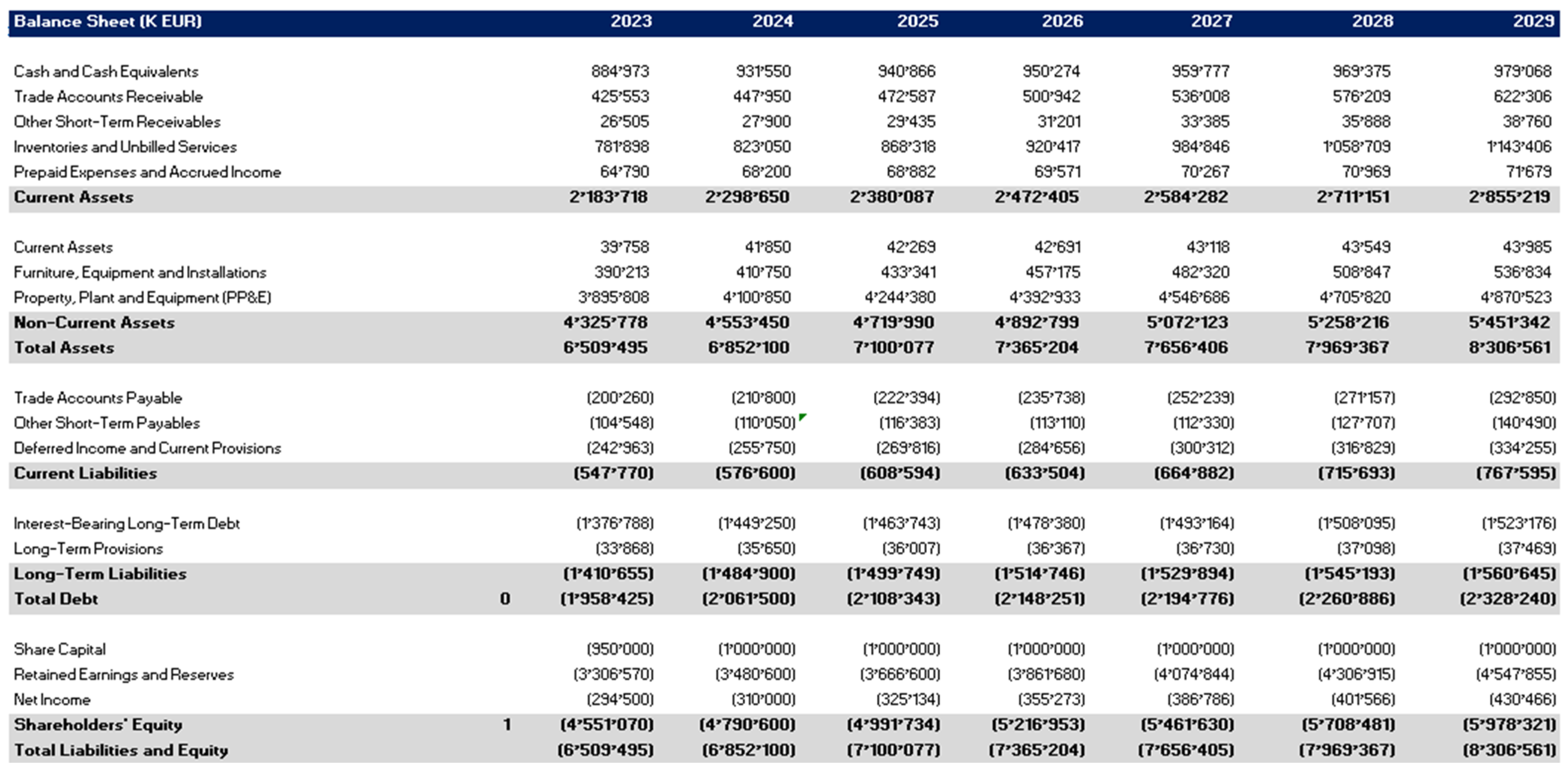
Figure A2.
Financial statements and projected financial information used in the Income Statement. Note: All amounts are expressed in K EUR. Negative amounts are presented in parentheses in accordance with the sign convention applied in the underlying financial model. Source: Authors’ own elaboration.
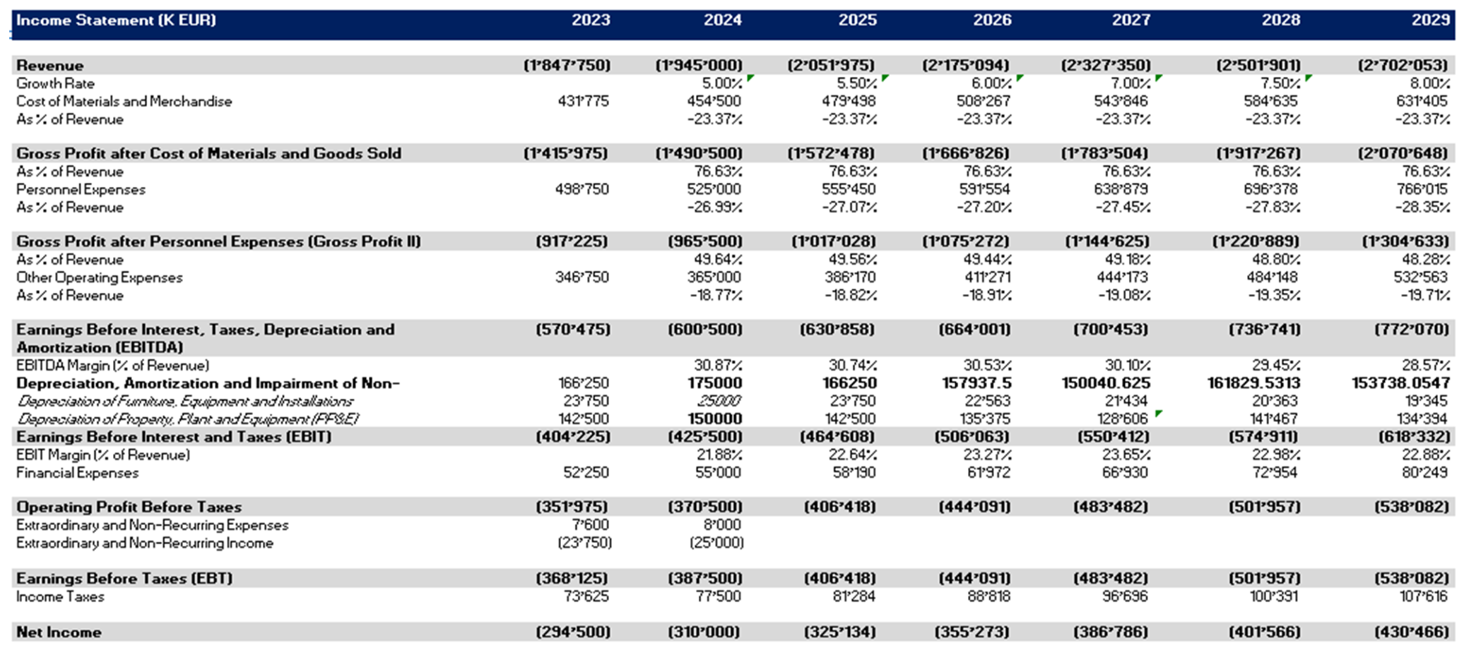
Figure A3.
Financial statements and projected financial information used in the Free Cash Flow to the Firm (FCFF). Note: All amounts are expressed in K EUR. Negative amounts are presented in parentheses in accordance with the sign convention applied in the underlying financial model.Source: Authors’ own elaboration.
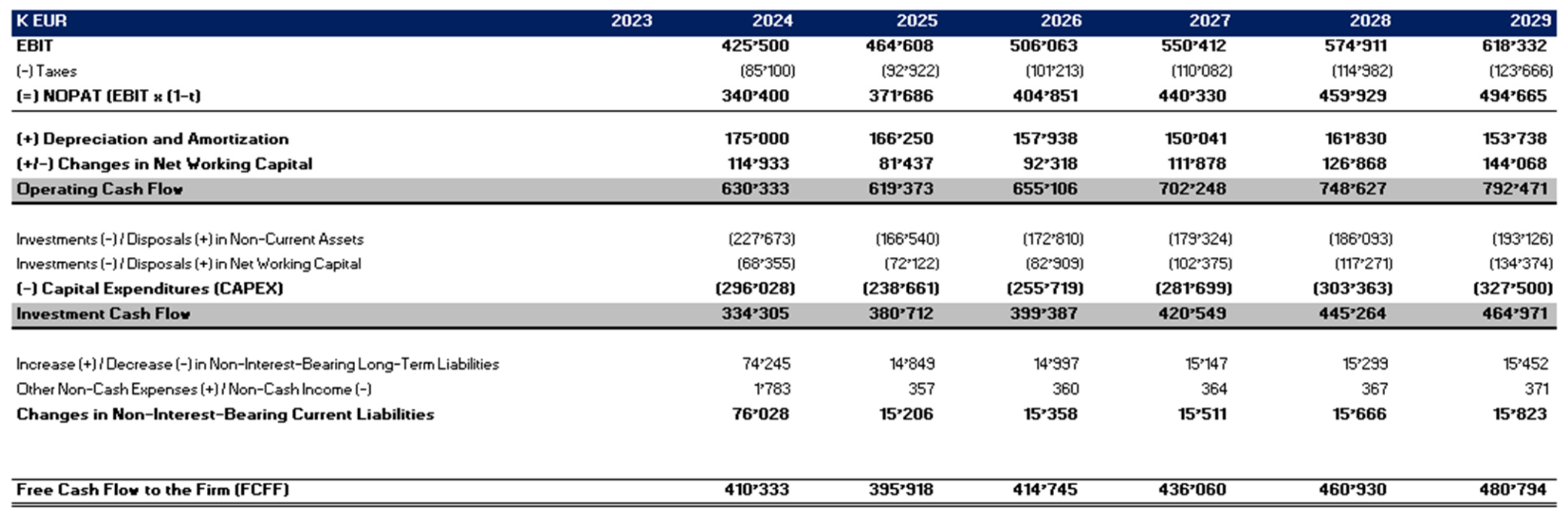
References
- Andrén, N., Jankensgård, H., & Oxelheim, L. (2005). Exposure-based cash-flow-at-risk: An alternative to VaR for industrial companies. Journal of Applied Corporate Finance, 17(3), 76–86. [Google Scholar] [CrossRef] [Scilit]
- Blum, U., Gleißner, W., Feldmann, B., & Fuhrmeister, C. (2018). Risikogerechte Beurteilung: Unternehmenswert und rating. In U. Blum, W. Gleißner, P. Nothnagel, & M. Veltins (Eds.), Vade mecum für Unternehmenskäufe (pp. 43–70). Springer Gabler. [Google Scholar]
- Bondarenko, S., Shlafman, N., Kuprina, N., Kalaman, O., Moravska, O., & Tsurkan, N. (2021). Planning, accounting and control as risk management tools for small business investment projects. Emerging Science Journal, 5(5), 650–666. [Google Scholar] [CrossRef] [Scilit]
- Brealey, R. A., Myers, S. C., & Allen, F. (2020). Principles of corporate finance (13th ed.). McGraw-Hill Education. [Google Scholar]
- Brick, I. E., & Weaver, D. G. (1984). A comparison of capital budgeting techniques in identifying profitable investments. Financial Management, 13(4), 29–39. [Google Scholar] [CrossRef] [Scilit]
- Chen, Y.-L., Chuang, Y.-W., Huang, H.-G., & Shih, J.-Y. (2020). The value of implementing enterprise risk management: Evidence from Taiwan’s financial industry. The North American Journal of Economics and Finance, 54, 100926. [Google Scholar] [CrossRef] [Scilit]
- Committee of Sponsoring Organizations of the Treadway Commission. (2013). Internal control—Integrated framework. Committee of Sponsoring Organizations of the Treadway Commission. [Google Scholar]
- Committee of Sponsoring Organizations of the Treadway Commission. (2017). Enterprise risk management—Integrating with strategy and performance. Committee of Sponsoring Organizations of the Treadway Commission. [Google Scholar]
- Copeland, T., Koller, T., & Murrin, J. (2000). Valuation: Measuring and managing the value of companies (3rd ed.). John Wiley & Sons. [Google Scholar]
- Damodaran, A. (2007). Valuation approaches and metrics: A survey of the theory and evidence. Foundations and Trends in Finance, 1(8), 693–784. [Google Scholar] [CrossRef] [Scilit]
- Damodaran, A. (2012). Investment valuation: Tools and techniques for determining the value of any asset (3rd ed.). John Wiley & Sons. [Google Scholar]
- Goehr, K., & Kupke, T. (2003). Unternehmensbewertung: Der Kapitalisierungszins im Rahmen der Unternehmensbewertung. Betriebswirtschaftliche Mandantenbetreuung, 10, 288–294. [Google Scholar]
- Guo, Y., Ge, H., Liao, Z., Hu, Y., & Huang, B. (2024). The influence of financial innovation on enterprise risk management. Finance Research Letters, 62, 105098. [Google Scholar] [CrossRef] [Scilit]
- Hadi, M. H., Abdulzahra, A. K., & Hazen, M. A. (2025). The effectiveness of internal control standards in enhancing financial risk management efficiency in the banking sector. European Journal of Management, Economics and Business, 2(5), 66–83. [Google Scholar] [CrossRef] [Scilit] [PubMed]
- Hering, T. (2021). Unternehmensbewertung (4th ed.). De Gruyter Oldenbourg. [Google Scholar]
- Hering, T. (2022). Investitionstheorie (6th ed.). De Gruyter Oldenbourg. [Google Scholar]
- Hertz, D. B. (1964). Risk analysis in capital investment. Harvard Business Review, 42(1), 95–106. [Google Scholar]
- Hopkin, P. (2018). Fundamentals of risk management: Understanding, evaluating and implementing effective risk management (5th ed.). Kogan Page. [Google Scholar]
- Hoyt, R. E., & Liebenberg, A. P. (2011). The value of enterprise risk management. Journal of Risk and Insurance, 78(4), 795–822. [Google Scholar] [CrossRef] [Scilit]
- Huang, L.-H. (2026). Evaluating the internal control strategy in the AI industry: Using the COSO framework. Applied Economics, 58(1), 172–185. [Google Scholar] [CrossRef] [Scilit]
- Indriastuti, M., Chariri, A., & Fuad, F. (2025). Enhancing firm value: The role of enterprise risk management, intellectual capital, and corporate social responsibility. Contaduría y Administración, 70(1), e486. [Google Scholar] [CrossRef] [Scilit]
- Kazlauskienė, V., & Christauskas, Č. (2007). Risk reflection in business valuation methodology. Engineering Economics, 1(51), 7–15. [Google Scholar]
- Khandelwal, C., Kumar, S., Tripathi, V., & Madhavan, V. (2023). Joint impact of corporate governance and risk disclosures on firm value: Evidence from emerging markets. Research in International Business and Finance, 66, 102022. [Google Scholar] [CrossRef] [Scilit]
- Koller, T., Goedhart, M., & Wessels, D. (2020). Valuation: Measuring and managing the value of companies (7th ed.). John Wiley & Sons. [Google Scholar]
- Kudla, R. J. (1980). Some pitfalls in using certainty-equivalents: A note. Journal of Business Finance & Accounting, 7(2), 239–243. [Google Scholar] [CrossRef] [Scilit]
- Li, F., Yao, Y., Lu, P., & Li, Y. (2025). Risk disclosure and company valuation: Moderating effect of regulation. Finance Research Letters, 82, 107636. [Google Scholar] [CrossRef] [Scilit]
- McKay, S. (2013). Risk assessment for mid-sized organisations: COSO tools for a tailored approach. Committee of Sponsoring Organizations of the Treadway Commission. [Google Scholar]
- Meitner, M., & Streitferdt, F. G. (2014). DCF valuations of companies in crisis: Distress-related leverage, identification of risk positions, discounting techniques, and “beta flips”. Journal of Business Valuation and Economic Loss Analysis, 9(1), 145–174. [Google Scholar] [CrossRef] [Scilit]
- Mohammed, M. A., Al-Abedi, T. K., Flayyih, H. H., & Mohaisen, H. A. (2021). Internal control frameworks and its relation with governance and risk management: An analytical study. Studies of Applied Economics, 39(11), 1–13. [Google Scholar] [CrossRef] [Scilit]
- Mun, J. (2006). Modeling risk: Applying Monte Carlo simulation, real options analysis, forecasting, and optimization techniques. John Wiley & Sons. [Google Scholar]
- Nielsen, S., & Pontoppidan, J. C. (2020). Exploring the inclusion of risk in management accounting and control. Management Research Review, 43(1), 82–112. [Google Scholar] [CrossRef] [Scilit]
- Nocco, B. W., & Stulz, R. M. (2006). Enterprise risk management: Theory and practice. Journal of Applied Corporate Finance, 18(4), 8–20. [Google Scholar] [CrossRef] [Scilit]
- Oh, H. M., Park, S. B., & Kim, J. H. (2020). Do analysts’ cash flow forecasts improve firm value? International Journal of Financial Studies, 8(4), 60. [Google Scholar] [CrossRef] [Scilit]
- Peng, Y., & Jin, H. (2025). Effects of information and technology application in audits and digital economy on enterprise risk management level. Finance Research Letters, 73, 106593. [Google Scholar] [CrossRef] [Scilit]
- Prewett, K., & Terry, A. (2018). COSO’s updated enterprise risk management framework—A quest for depth and clarity. Journal of Corporate Accounting & Finance, 29(3), 16–23. [Google Scholar] [CrossRef] [Scilit]
- Rappaport, A. (1998). Creating shareholder value: A guide for managers and investors (2nd ed.). Free Press. [Google Scholar]
- Razali, M. N., Jalil, R. A., Achu, K., & Ali, H. M. (2022). Identification of risk factors in business valuation. Journal of Risk and Financial Management, 15(7), 282. [Google Scholar] [CrossRef] [Scilit]
- Shin, I., & Park, S. (2017). Integration of enterprise risk management and management control system: Based on a case study. Investment Management and Financial Innovations, 14(1), 19–26. [Google Scholar] [CrossRef] [Scilit]
- Spira, L. F., & Page, M. (2003). Risk management: The reinvention of internal control and the changing role of internal audit. Accounting, Auditing & Accountability Journal, 16(4), 640–661. [Google Scholar] [CrossRef] [Scilit]
- Stein, J. C., Usher, S. E., LaGattuta, D., & Youngen, J. (2001). A comparables approach to measuring cash flow-at-risk for non-financial firms. Journal of Applied Corporate Finance, 13(4), 8–17. [Google Scholar] [CrossRef] [Scilit]
- Turgaeva, A. A. (2024). Assessment of components of the internal control system for the purpose of risk management of organizations. Economic Problems and Legal Practice, 20(4), 251–257. [Google Scholar] [CrossRef] [Scilit]
- Wibowo, J. C., Ariefianto, M. D., Laurence, L., & Soepriyanto, G. (2025). Resilience, valuation, and governance interactions in shaping financial accounting manipulation: Evidence from Asia. Journal of Risk and Financial Management, 18(12), 719. [Google Scholar] [CrossRef] [Scilit]
- Yun, J. (2023). The effect of enterprise risk management on corporate risk management and firm performance. Finance Research Letters, 55, 103950. [Google Scholar] [CrossRef] [Scilit]
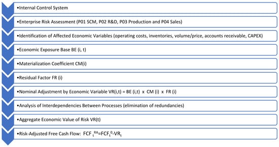
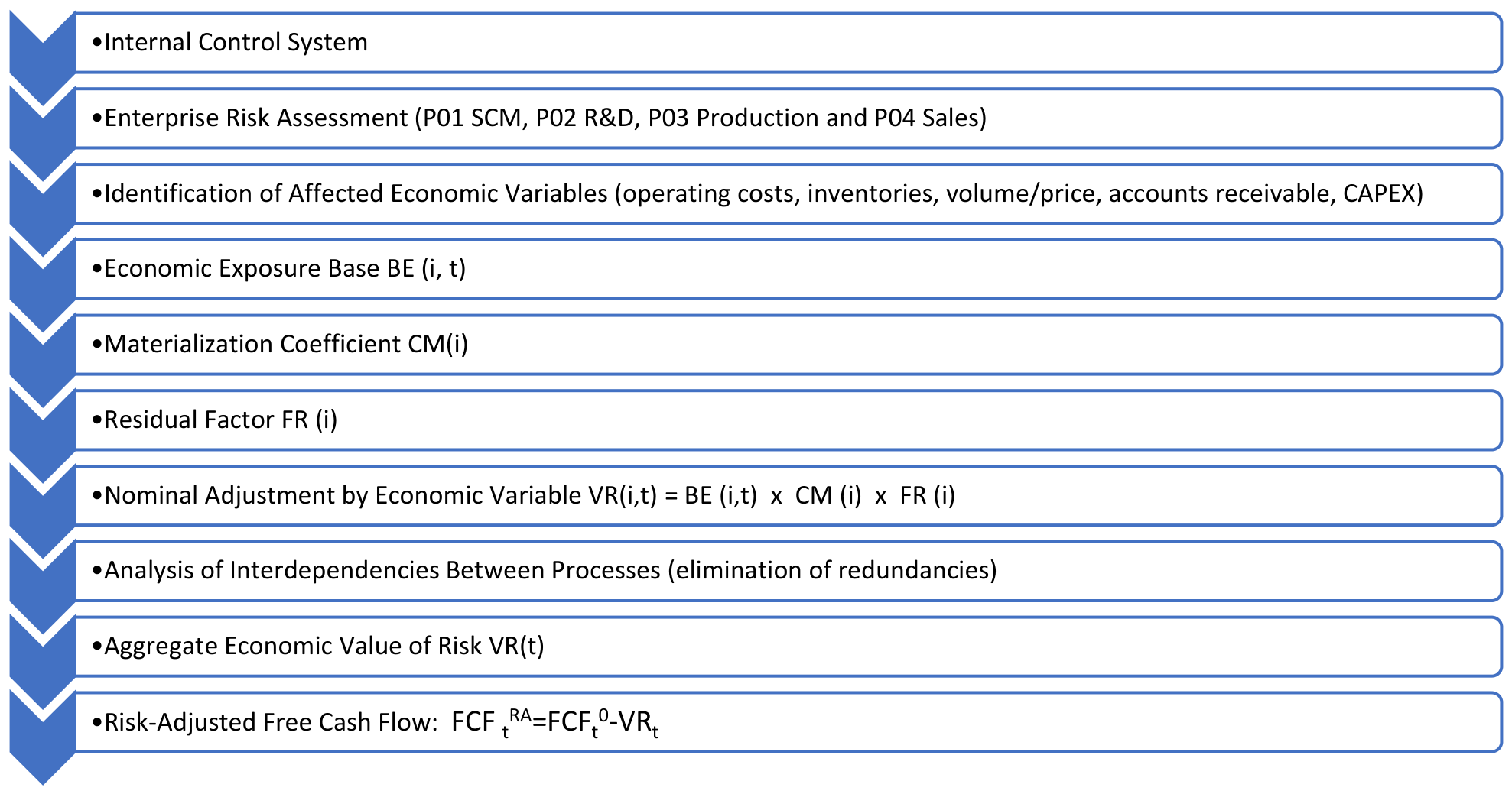
Disclaimer/Publisher’s Note: The statements, opinions and data contained in all publications are solely those of the individual author(s) and contributor(s) and not of MDPI and/or the editor(s). MDPI and/or the editor(s) disclaim responsibility for any injury to people or property resulting from any ideas, methods, instructions or products referred to in the content. |
© 2026 by the authors. Licensee MDPI, Basel, Switzerland. This article is an open access article distributed under the terms and conditions of the Creative Commons Attribution (CC BY) license.