Article

Economic Growth and Carbon Emissions in Croatia and Albania: Evidence from Annual and Medium-Term Decoupling Patterns

by
Mirjana Jeleč Raguž
1,*,
Elenica Pjero Beqiraj
2 and
Ariana Ergović
1
1
Faculty of Tourism and Rural Development in Pozega, Josip Juraj Strossmayer University of Osijek, 34000 Pozega, Croatia
2
Faculty of Economy, University of Vlora “Ismail Qemali”, 9401 Vlore, Albania
*
Author to whom correspondence should be addressed.
J. Risk Financ. Manag. 2026, 19(9), 737; https://doi.org/10.3390/jrfm19090737
Submission received: 19 August 2026 / Revised: 13 September 2026 / Accepted: 13 September 2026 / Published: 16 September 2026
(This article belongs to the Section Economics and Finance)

Abstract

This study examines the relationship between economic growth and CO2 emissions in Croatia and Albania from 1995 to 2024, using the EU27 as a benchmark. The analysis combines carbon intensity trends, Mann–Kendall tests, Sen’s slope estimates, Tapio decoupling elasticities, and a supplementary LMDI decomposition. Contiguous intervals and rolling five-year windows, together with threshold, near-zero GDP, and alternative emissions-source checks, assess temporal consistency and robustness. Carbon intensity declined significantly in all three cases, but decoupling outcomes differed across time horizons. Favorable annual decoupling occurred in 44.8% of observations in Croatia, 55.2% in Albania, and 69.0% in the EU27, while the corresponding descriptive shares across the overlapping five-year windows were 64.0%, 56.0%, and 92.0%. The differences in favorable annual decoupling shares were not statistically significant. The LMDI results indicate that improved energy intensity offset part of the emissions pressure associated with economic activity in Croatia and Albania, while Albania’s carbon-intensity-of-energy effect was close to zero. Annual decoupling results were more sensitive to the emissions source than the medium-term comparison. CBAM-covered products accounted for 14.02% of EU27 imports from Albania in 2024. Overall, the results show that assessments of low-carbon transition progress can differ with the time horizon considered and that domestic decoupling may coexist with trade exposure to carbon regulation.

1. Introduction

The European Union (EU) has established ambitious targets for reducing greenhouse gas emissions (European Parliament & Council of the European Union, 2021) while pursuing economic growth that is increasingly decoupled from resource use (European Commission, 2019). This raises an important question of whether economic activity can continue to grow without a corresponding increase in environmental pressure and, more specifically, whether growth can occur while CO2 emissions decline. The question is particularly relevant for transition economies, where changes in economic structure, energy systems, and economic activity have often been accompanied by considerable changes in emissions.
Decoupling provides a useful framework for examining this relationship. Relative, or weak, decoupling occurs when GDP and emissions both increase but emissions grow more slowly than economic activity, whereas absolute, or strong, decoupling occurs when GDP increases while emissions decline (Tapio, 2005). This distinction is important because a decline in carbon intensity does not necessarily imply a decline in total emissions. An economy may produce less CO2 per unit of output while its overall emissions continue to increase. Carbon intensity and the relationship between changes in GDP and emissions therefore capture different, but complementary, aspects of decarbonization.
Croatia and Albania provide a useful comparative setting as two small European transition economies that share a broader post-socialist development context but differ in their institutional relationship with the European Union. Croatia has been an EU Member State since 2013, whereas Albania remains an EU candidate country. Their comparison therefore provides a focused setting for examining whether decoupling patterns across different time horizons show similar temporal characteristics in two transition economies at different stages of European integration. The EU27 is used as an aggregate benchmark representing the broader European decarbonization trajectory rather than as a directly comparable third economy. This comparison allows developments in Croatia and Albania to be considered against the wider European trajectory without attributing observed differences to EU membership itself.
The decoupling approach is related to, but distinct from, the Environmental Kuznets Curve (EKC). While the EKC examines how environmental pressure changes with the level of economic development, decoupling analysis focuses more directly on changes in economic activity relative to changes in emissions over time (Dinda, 2004; Tapio, 2005). This is particularly useful for smaller transition economies, where recessions, rapid growth, structural changes, and external shocks may generate substantial year-to-year variation in both GDP and emissions. Annual observations can therefore reveal changes that may be obscured by long-term trends, but they may also provide a different picture from that observed over broader time horizons.
Existing research shows substantial progress in decoupling across European economies but also considerable variation across countries and periods. Evidence for transition economies is less uniform, with changes in emissions often remaining closely related to economic activity and energy use (Pejović et al., 2021; Ziemblińska et al., 2025; Zhigolli & Fetai, 2024). Evidence for Croatia and Albania is more limited and fragmented. Studies for Croatia have mainly examined the EKC or particular economic sectors (Ahmad et al., 2017; Jeleč Raguž, 2026; Jeleč Raguž et al., 2026), while research for Albania points to the importance of energy consumption and renewable energy for emissions (Mulaj, 2025). Direct comparative evidence on how decoupling patterns in these two economies differ between annual and medium-term horizons remains scarce.
This study addresses this issue by examining real GDP, CO2 emissions, and carbon intensity in Croatia and Albania over the period 1995–2024, using the EU27 as a benchmark. Long-term carbon intensity trends are considered together with annual Tapio decoupling states and medium-term decoupling patterns based on contiguous medium-term intervals and rolling five-year windows. The use of different time horizons makes it possible to distinguish the frequency of favorable annual decoupling from its temporal consistency over the medium term. A supplementary LMDI decomposition is used to examine the contributions of economic activity, energy intensity, and the carbon intensity of energy to changes in energy sector CO2 emissions. For Albania, the analysis is additionally complemented by an indicator of trade exposure to products covered by the EU Carbon Border Adjustment Mechanism (CBAM), adding a regulatory transition risk dimension to the assessment without treating trade exposure as an estimate of financial CBAM costs.
Against this background, the main contribution of the study lies in distinguishing between the frequency of favorable annual decoupling and its temporal consistency over medium-term horizons. By comparing Croatia and Albania, the analysis shows whether conclusions based on year-to-year decoupling remain consistent when the growth–emissions relationship is assessed over longer periods. Accordingly, the study addresses the following research questions:
RQ1: How have real GDP, CO2 emissions, and carbon intensity developed in Croatia and Albania relative to the EU27 since 1995?
RQ2: What types of decoupling between economic growth and CO2 emissions can be identified in Croatia, Albania, and the EU27 over the observed period?
RQ3: To what extent are favorable decoupling patterns temporally consistent across medium-term horizons in Croatia and Albania relative to the EU27 benchmark?
RQ4: To what extent is Albania’s trade with the EU exposed to CBAM-covered product categories, and which sectors account for this exposure?
The supplementary LMDI decomposition adds an analytical dimension by identifying the relative contributions of economic activity, energy intensity, and the carbon intensity of energy to changes in energy sector CO2 emissions. This perspective complements existing evidence by showing how conclusions about decoupling may depend on the time horizon over which the growth–emissions relationship is assessed. The comparison of Croatia and Albania adds evidence for two relatively under-researched transition economies, while the supplementary CBAM analysis connects Albania’s domestic decoupling performance with its trade-related exposure to EU carbon regulation.
The remainder of the study is organized as follows. Section 2 reviews the relevant literature. Section 3 describes the data and methodology. Section 4 presents the empirical results. Section 5 discusses the findings, their implications, and the limitations of the analysis, while Section 6 concludes the study.

2. Literature Review

2.1. Conceptual Foundations: EKC, Decoupling, and Carbon Intensity

The relationship between economic growth and environmental pressure has traditionally been examined through the Environmental Kuznets Curve (EKC), which proposes a non-linear relationship between income and environmental degradation (Grossman & Krueger, 1995; Stern, 2004). Empirical support for the EKC, however, is sensitive to model specification and the period considered, encouraging the use of approaches that examine changes in economic activity and emissions more directly (Dinda, 2004).
One of these approaches is the concept of decoupling. The OECD (2002) introduced decoupling as a framework for assessing whether environmental pressures can be separated from economic growth, while Tapio (2005) developed an elasticity-based classification that distinguishes different states of coupling and decoupling during both economic expansion and contraction. This distinction matters because falling emissions during economic contraction cannot be interpreted in the same way as falling emissions during economic growth. Absolute decoupling, in which economic growth occurs alongside declining emissions, remains limited in scope and duration internationally (Vadén et al., 2020).
The EKC and decoupling frameworks address related but different questions. The EKC concerns the shape of the relationship between environmental pressure and income levels, whereas decoupling examines whether changes in environmental pressure become separated from changes in economic activity over a specified period. Green-growth and ecological-modernization perspectives provide broader theoretical frameworks for understanding how economic development may be reconciled with reduced environmental pressures (Mol et al., 2009; OECD, 2011). In the context of CO2 emissions, this may involve improvements in energy efficiency, technological progress, changes in the energy mix, and structural shifts toward less carbon-intensive activities. These mechanisms are also central to the energy transition literature, but their presence cannot be inferred from a favorable decoupling classification alone. Decoupling should therefore be interpreted as an observed growth–emissions relationship rather than, by itself, evidence of the technological or structural mechanisms that produced it.
Empirical studies provide support for the relevance of these factors, although they examine broader environmental and sustainability outcomes rather than decoupling itself. Eco-innovation has been associated with a lower ecological footprint in China (Zhang et al., 2025), while energy technology innovation has been linked to sustainable development in OECD economies (Khan et al., 2025a). Evidence from advanced economies also points to the relevance of economic complexity, renewable energy, and adaptation technologies for sustainable development and environmental quality (Khan & Subhan, 2026; Khan et al., 2025b).
Carbon intensity provides a complementary, but distinct, measure. Declining CO2 emissions per unit of GDP indicate that production is becoming less carbon-intensive, but total emissions may still increase if economic growth outweighs efficiency gains. Shuai et al. (2019), examining 133 countries over 2000–2014, found that decoupling economic growth from carbon intensity was considerably more widespread than decoupling growth from total carbon emissions. A decline in carbon intensity should therefore not be treated as equivalent to absolute decoupling.

2.2. Time Horizons and Temporal Consistency in Decoupling

The time horizon of the analysis is also important. Annual Tapio elasticities capture year-to-year changes but are sensitive to short-term economic fluctuations. Cohen et al. (2022) distinguish longer-run trends from short-run cyclical movements in the growth–emissions relationship, while previous decoupling studies have used longer periods (R. Xie et al., 2022) or combined annual and multi-year changes (Han et al., 2022). Hubacek et al. (2021) found that countries displaying absolute decoupling in one period did not necessarily maintain the same pattern in a subsequent period, while Kilinc-Ata et al. (2026) emphasize the consistency of decoupling across time rather than its occurrence in isolated years. Assessing more than one time horizon can therefore help distinguish the frequency of favorable annual outcomes from their temporal consistency over broader periods, although multi-year analysis should not be interpreted as a formal test of persistence.
The distinction between annual and medium-term assessment is particularly relevant because the two horizons capture different features of the growth–emissions relationship. Annual classifications are more responsive to short-term changes in economic activity, energy demand, and emissions, whereas multi-year comparisons can reveal whether a favorable relationship remains visible when such fluctuations are considered over a broader period. Consequently, an economy may record a relatively limited number of favorable annual observations while still exhibiting a more favorable growth–emissions relationship over medium-term horizons, or vice versa. Examining both perspectives can therefore provide a more complete assessment of decoupling performance than relying on annual classifications alone.

2.3. Evidence from Europe and Transition Economies

At the European level, research indicates substantial progress in decoupling economic growth from CO2 emissions, alongside considerable differences among countries (Bianco et al., 2024; Cautisanu & Hatmanu, 2023; Q. Xie et al., 2025). Broader international evidence shows that decoupling remains uneven across countries and regions, with more favorable patterns observed in Europe than in most other regions (Freire-González et al., 2024/2024). At the same time, absolute decoupling should not necessarily be equated with green growth: evidence from high-income countries shows that reductions in consumption-based CO2 emissions achieved alongside economic growth can fall well short of rates consistent with climate targets (Vogel & Hickel, 2023). Comparisons between the EU and other regions also indicate differences in the temporal consistency of decoupling (Kilinc-Ata et al., 2026). Aggregate EU performance should therefore be understood as a broad reference trajectory rather than evidence that individual European economies follow the same pattern.
Evidence for transition economies is less uniform. Emission reductions may coincide with economic fluctuations rather than sustained changes in the growth–emissions relationship (Brizga et al., 2014; Ziemblińska et al., 2025). Studies of the Western Balkans report positive relationships between economic growth, energy consumption, and CO2 emissions, highlighting the continuing importance of economic expansion and energy use for emissions (Pejović et al., 2021; Zhigolli & Fetai, 2024).
For Croatia, much of the existing literature has focused on the EKC. Ahmad et al. (2017) and Jeleč Raguž (2026) report evidence consistent with an inverted U-shaped relationship between income and CO2 emissions, whereas Ziemblińska et al. (2025) do not find sufficient evidence that Croatia has reached the downward-sloping segment of the EKC. Sectoral evidence further shows that national trends may conceal substantial heterogeneity: Jeleč Raguž et al. (2026) find differences in carbon intensity and decoupling across tourism-related sectors, including accommodation and individual transport modes. These differing findings illustrate the sensitivity of conclusions about Croatia’s growth–emissions relationship to the analytical framework, period, and specification used, and provide an additional reason to examine decoupling directly rather than infer it from the estimated EKC shape. Country-specific evidence for Albania remains limited. Available research indicates that the relationship between economic growth and CO2 emissions may differ between the short and long run, with energy consumption contributing to emissions and renewable energy associated with lower emissions (Mulaj, 2025).
Taken together, the literature provides evidence on carbon intensity and decoupling across Europe and transition economies, but direct comparative evidence for Croatia and Albania remains limited. More importantly, less is known about whether conclusions based on the frequency of favorable annual decoupling remain consistent when the same growth–emissions relationship is assessed over medium-term horizons. This study addresses that gap by combining long-term carbon intensity trends with annual Tapio classifications and contiguous medium-term intervals and rolling five-year windows for Croatia and Albania over 1995–2024, using the EU27 as an aggregate benchmark. The design allows annual decoupling frequency and medium-term temporal consistency to be examined as related but distinct dimensions of decoupling performance.

3. Data and Methodology

3.1. Data and Variables

For the purpose of this study, annual data for Croatia, Albania, and the European Union (EU27) covering the period 1995–2024 are used in the analysis. The baseline data for the core analysis were obtained from the World Bank World Development Indicators (WDI) database. The WDI series is retained as the baseline because it provides a harmonized source for Croatia, Albania, and the EU27 over the full study period, while the EEA inventory series is used as an alternative specification to assess source sensitivity. The starting year was selected primarily to avoid war-related disruptions and the strongest early-transition distortions, particularly in Croatia, while providing a sufficiently long and comparable period for the two countries.
Three variables are included in the core analysis: real gross domestic product (GDP), total CO2 emissions, and carbon intensity. Real GDP is expressed in constant 2015 US dollars (World Bank, 2026b) and is used to measure economic activity independently of price changes. CO2 emissions are expressed in million tons of CO2 equivalent (Mt CO2e) (World Bank, 2026a) and refer to total carbon dioxide emissions excluding land use, land use change, and forestry (LULUCF). Carbon intensity is calculated as the ratio of CO2 emissions to real GDP.
For the alternative-source robustness check, CO2 emissions data were additionally obtained from the European Environment Agency (EEA) Greenhouse Gases Data Viewer (EEA, 2026). The EEA series corresponds to the “Total emissions (UNFCCC)” CO2 category, excluding LULUCF, and covers the same 1995–2024 period. These data are used only as an alternative emissions specification; the World Bank real GDP series is retained throughout the robustness analysis. For the supplementary consumption-based robustness check, Croatia’s CO2 emission footprint was obtained from Eurostat’s FIGARO carbon dioxide emission footprints dataset (env_ac_co2fp). The series attributes CO2 emissions along global production chains to final demand and, using the aggregate for all NACE activities plus households, is available for the 2010–2023 period used in this check (Eurostat, 2026a). The consumption-based robustness check is restricted to Croatia because a comparable consumption-based CO2 emissions series is not available for Albania in the FIGARO dataset.
For the supplementary LMDI decomposition, total energy supply (TES) was obtained from Eurostat energy balances and is measured in thousand tons of oil equivalent (ktoe) (Eurostat, 2026c). Energy sector CO2 emissions were obtained from the EEA Greenhouse Gases Data Viewer using the IPCC Sector 1 (Energy) CO2 series for Croatia, Albania, and the EU27 (EEA, 2026). The decomposition covers the same 1995–2024 period. The use of Sector 1 emissions in this supplementary analysis provides a closer correspondence between the emissions measure and the energy variable used in the decomposition.
The EU27 series represents the current membership composition retrospectively over the full period, with the United Kingdom excluded throughout. Croatia is therefore included in the EU27 aggregate throughout the series, although its weight in the aggregate is small. This should be kept in mind when interpreting comparisons between the two national economies and the EU27 benchmark.
Total GDP and total CO2 emissions are used rather than per capita measures because the study focuses on economy-wide decoupling between aggregate economic activity and total territorial emissions. Per capita indicators would address a related but different question by incorporating population dynamics and are therefore outside the scope of the present analysis.
Carbon intensity is calculated as:
C I t =   C O 2 , t G D P t
where CIt represents carbon intensity in year t, CO2,t represents total CO2 emissions, and GDPt represents real GDP. A decline in carbon intensity means that less CO2 is emitted per unit of economic output. It therefore indicates an improvement in the emission efficiency of the economy but not necessarily absolute decoupling, since total emissions may still increase when GDP grows more rapidly.
For the supplementary analysis of regulatory transition exposure, bilateral trade data were obtained from Eurostat Comext (dataset DS-059322, EU trade since 2002 by HS2-4-6 and CN8) for the period 2015–2024 (Eurostat, 2026b). The EU27 was specified as the reporting area, Albania as the partner country, and imports as the trade flow, with trade values expressed in euros. Both the numerator and denominator of the exposure measure were therefore constructed from the same reporting perspective and data source.
CBAM-covered trade was identified using the product scope defined in Annex I to Regulation (EU) 2023/956 (European Parliament & Council of the European Union, 2023). Annual import values for these product groups were subsequently compared with total annual EU27 imports from Albania.

3.2. Analytical Approach

The empirical analysis combines long-term trend assessment with annual and medium-term measures of decoupling. Long-term changes in carbon intensity are first examined using indexed trends and non-parametric trend methods. The relationship between economic growth and CO2 emissions is then assessed using the Tapio elasticity framework at annual and medium-term horizons. Statistical comparisons and sensitivity checks are used to examine the robustness of the resulting decoupling patterns. An LMDI decomposition is additionally used to examine the contributions of economic activity, energy intensity, and the carbon intensity of energy to changes in energy sector CO2 emissions. The supplementary CBAM analysis presented in Section 3.3 adds a regulatory transition risk perspective for Albania.
Long-term developments in GDP, CO2 emissions, and carbon intensity are first presented as index series, with 1995 set as the base year (1995 = 100). Indexing allows the relative trajectories of variables measured in different units to be compared across Croatia, Albania, and the EU27 despite substantial differences in their initial levels. This provides a descriptive indication of whether economic growth and emissions have moved together over time or have increasingly diverged.
The long-term trend in carbon intensity is subsequently examined using the Mann–Kendall trend test (Mann, 1945) and Sen’s slope estimator (Sen, 1968). The Mann–Kendall test is a non-parametric procedure for detecting monotonic trends and does not require observations to follow a normal distribution. Sen’s slope complements the test by estimating the direction and magnitude of the trend. Statistical significance is assessed at the 5% level.
Because serial autocorrelation can affect inference from the Mann–Kendall test, first-order serial autocorrelation is assessed for each carbon intensity series after detrending. Where significant autocorrelation is detected, the Trend-Free Pre-Whitening (TFPW) procedure of Yue et al. (2002) is applied before performing the Mann–Kendall test. The Mann–Kendall test is therefore conducted on the TFPW-adjusted series, while Sen’s slope is estimated from the original time series.
The trend analysis is supplemented by several robustness diagnostics. Lag-1 autocorrelation is reported for each carbon intensity series, and statistical significance is additionally assessed using the Hamed–Rao modified Mann–Kendall test (Hamed & Rao, 1998), which adjusts the variance of the test statistic for serial dependence. This provides an alternative treatment of autocorrelation and makes it possible to assess whether the inference on the direction and significance of the trend is robust to the method used to address serial dependence. Sen’s slope is also reported with its 95% confidence interval.
Since absolute Sen slopes are affected by differences in carbon intensity levels, the slope is additionally expressed relative to mean carbon intensity:
R S i =   β i C I i ¯   ×   100
where RSi denotes the relative Sen slope for economy i, βi is the corresponding Sen slope, and C I ¯ i is mean carbon intensity over the study period. The resulting measure expresses the estimated annual trend as a percentage of the economy’s average carbon intensity level and facilitates comparison across the three economies.
Annual decoupling between changes in real GDP and CO2 emissions is examined using the Tapio elasticity approach (Tapio, 2005). Whereas the preceding analysis focuses on longer-term developments in carbon intensity, the Tapio framework captures changes in the relationship between economic activity and emissions from one period to another. The decoupling index is calculated as:
D I t =   % C O 2 , t % G D P t
where DIt denotes the decoupling index in year t, while % C O 2 , t and % G D P t denote the annual percentage changes in CO2 emissions and real GDP, respectively.
The interpretation of the index depends on both its value and the direction of change in GDP and emissions. The same elasticity value may therefore correspond to a different decoupling state depending on whether the economy is expanding or contracting. Following Tapio (2005), observations are classified into eight decoupling states using the conventional threshold values of 0.8 and 1.2, as shown in Table 1. Because annual changes require a preceding-year observation, the annual analysis comprises 29 observations for each economy, covering 1996–2024.
Strong decoupling represents the most favorable state, as real GDP increases while absolute CO2 emissions decline. Weak decoupling also represents a favorable outcome, although emissions continue to increase at a slower rate than GDP. For the comparative frequency analysis, strong and weak decoupling are therefore grouped as favorable decoupling outcomes. The remaining categories distinguish between different forms of coupling and negative decoupling during periods of economic expansion or contraction. This distinction is relevant over a period that includes recessions and major external shocks, since a decline in emissions during an economic contraction does not carry the same interpretation as declining emissions alongside economic growth.
The annual analysis reports the frequency and share of each Tapio state for Croatia, Albania, and the EU27. Favorable annual shares are compared using pairwise two-proportion tests, supplemented by an omnibus chi-square test of differences across the three economies. These tests are used to distinguish descriptive differences in annual frequencies from statistically supported differences in proportions.
The annual analysis is then extended to a medium-term horizon. Changes in GDP and CO2 emissions are calculated over six contiguous endpoint intervals: 1995–2000, 2000–2005, 2005–2010, 2010–2015, 2015–2020, and 2020–2024. For each interval, the percentage change in CO2 emissions is related to the percentage change in real GDP and classified according to the same eight Tapio states used in the annual analysis. The final interval covers four rather than five years because 2024 is the last year in the dataset. These intervals are used as a descriptive medium-term diagnostic rather than as a formal test of persistence.
To reduce dependence on a small number of fixed endpoints, the medium-term analysis is supplemented with rolling five-year windows. The rolling specification covers 25 overlapping intervals, from 1995–2000 to 2019–2024, with the observation window moving forward by one year at a time. This provides a broader view of whether the decoupling pattern remains similar when the timing of the five-year period changes. However, adjacent rolling windows share four years of observations and are therefore not statistically independent. For this reason, the frequency of favorable outcomes across the rolling windows is treated as a descriptive measure of temporal consistency rather than used for inferential comparisons of proportions. The rolling-window analysis is thus intended to assess the medium-term stability of the observed decoupling patterns rather than to provide a formal statistical test of persistence.
The robustness of the Tapio classifications is examined in two additional ways. First, the conventional 0.8/1.2 thresholds are compared with narrower 0.9/1.1 and wider 0.7/1.3 specifications. The alternative thresholds are applied to both the annual observations and the rolling five-year windows. This makes it possible to assess whether the comparative pattern of favorable decoupling depends materially on the conventional boundary values used to distinguish the Tapio states.
Second, particular attention is given to observations in which the change in GDP is close to zero. Since GDP growth appears in the denominator of the Tapio elasticity, very small changes in GDP can generate large elasticity values and potentially unstable classifications. Observations for which |ΔGDP| < 0.5% are therefore identified in both the annual and rolling analyses. Favorable decoupling shares are recalculated after excluding these observations and compared with the baseline results. The observations are retained in the main analysis; their exclusion serves only as a sensitivity check on whether near-zero GDP changes materially affect the comparative findings.
Taken together, the different analytical components capture related but distinct aspects of the growth–emissions relationship. The carbon intensity analysis identifies the direction and rate of long-term change, while the annual Tapio classifications show how frequently favorable decoupling occurs from year to year. The contiguous and rolling analyses provide a medium-term perspective on the stability of these patterns, and the sensitivity checks indicate how strongly the classifications depend on threshold choice and near-zero GDP changes. This distinction is important because a relatively high frequency of favorable annual outcomes does not necessarily imply that decoupling is equally stable across longer time horizons.
Finally, source sensitivity is assessed by repeating the main analysis using the alternative EEA CO2 series described in Section 3.1 while retaining the World Bank real GDP series. Carbon intensity trends, annual Tapio classifications, rolling five-year windows, and contiguous medium-term intervals are recalculated for Croatia, Albania, and the EU27.
As a supplementary robustness check, production-based and consumption-based CO2 outcomes were compared for Croatia over their common 2010–2023 period. Consumption-based emissions were used to assess whether the decoupling results are sensitive to emissions embodied in international trade. Using the same real GDP series, carbon intensity changes and annual Tapio classifications were recalculated with the consumption-based CO2 series and compared with the corresponding production-based results.
To provide a more direct decomposition of the factors associated with changes in energy-related CO2 emissions, an additive Logarithmic Mean Divisia Index (LMDI-I) decomposition based on the Kaya identity was applied following Ang (2005). The additive LMDI-I formulation provides an exact decomposition without a residual term (Ang, 2005). Energy sector CO2 emissions were expressed as the product of real GDP, energy intensity, and the carbon intensity of energy:
C O 2 =   G D P   ×   T E S G D P   ×   C O 2 T E S
where TES denotes total energy supply. The change in energy sector CO2 emissions was decomposed into three additive components: an activity effect, reflecting changes in real GDP; an energy intensity effect, reflecting changes in TES per unit of GDP; and a carbon-intensity-of-energy effect, reflecting changes in energy sector CO2 emissions per unit of TES.
The decomposition covers 1995–2024 for Croatia, Albania, and the EU27 using the GDP, TES, and energy sector CO2 series described in Section 3.1. The main decomposition compares the 1995 and 2024 endpoints, while annual decompositions are used as a supplementary diagnostic of changes over time.

3.3. CBAM Trade Exposure Analysis

To complement the decoupling analysis with a regulatory transition risk perspective, a descriptive CBAM trade exposure indicator is constructed for Albania. The analysis is restricted to Albania because, unlike Croatia, it is a non-EU trading partner whose exports to the EU fall within the external scope of the mechanism, whereas Croatia, as an EU Member State, operates within the EU’s internal carbon-pricing framework. The indicator measures the share of annual EU27 imports from Albania that falls within the product scope of the Carbon Border Adjustment Mechanism (CBAM). For each year t, CBAM trade exposure is calculated as:
C B A M   E x p o s u r e t =   C B A M c o v e r e d   i m p o r t s t T o t a l   E U 27   i m p o r t s   f r o m   A l b a n i a t   ×   100
where CBAM-covered importst denotes the value of EU27 imports from Albania falling within the product scope of Annex I to Regulation (EU) 2023/956, and Total EU27 imports from Albaniat denotes the total value of EU27 imports from Albania in the same year.
Product coverage is operationalized using the Combined Nomenclature (CN) codes specified in Annex I to Regulation (EU) 2023/956. The relevant codes are assigned to the six CBAM sectors covered by the Regulation: cement, electricity, fertilizers, iron and steel, aluminum, and hydrogen. Where an Annex I heading contains an explicit exclusion, the corresponding non-covered products are removed where the available CN classification permits this. In particular, the exclusions specified within Chapter 72 for iron and steel, including ferrous waste and scrap (CN 7204) and the excluded ferro-alloy categories, are removed from the CBAM-covered trade values. The explicit exclusion of CN 3105 60 00 from the fertilizer category is treated in the same way. This procedure avoids including products outside the regulatory scope and reduces the risk of double counting.
In addition to the aggregate exposure ratio, sector-specific exposure shares are calculated by dividing the annual value of imports in each CBAM sector by total EU27 imports from Albania. The sectoral breakdown is used to identify which product groups account for the observed level and changes in overall CBAM trade exposure.
The indicator should not be interpreted as an estimate of Albania’s actual financial burden under CBAM. Such an estimate would require product-level information on embedded emissions, the applicable EU carbon price, and any carbon price effectively paid in the country of origin. The measure used here instead captures the share of Albania’s exports to the EU that falls within product categories directly covered by the CBAM framework. It is therefore interpreted as an indicator of regulatory trade exposure relevant to transition risk assessment rather than as a measure of monetary compliance costs.
A minor product-mapping limitation concerns CN code ex 2507 00 80 in the current CBAM product scope. The “ex” designation means that only part of the corresponding CN8 category is covered, while the historical Comext data used here do not allow the covered subcomponent to be isolated consistently over the full 2015–2024 period. The full CN8 category is therefore retained in the mapping. Given its very small contribution to total CBAM exposure, this limitation is unlikely to materially affect the overall results.


4. Results

The results are presented in six parts. The analysis begins with long-term developments in GDP, CO2 emissions, and carbon intensity in Croatia, Albania, and the EU27, followed by annual and medium-term Tapio decoupling patterns. The robustness of the decoupling results is then examined through sensitivity analyses and an alternative emissions data source. An LMDI decomposition examines the energy-related drivers of emissions changes, while the final section presents Albania’s trade exposure to CBAM-covered products as a supplementary regulatory transition risk indicator.

4.1. Long-Term Trends in GDP, CO2 Emissions, and Carbon Intensity

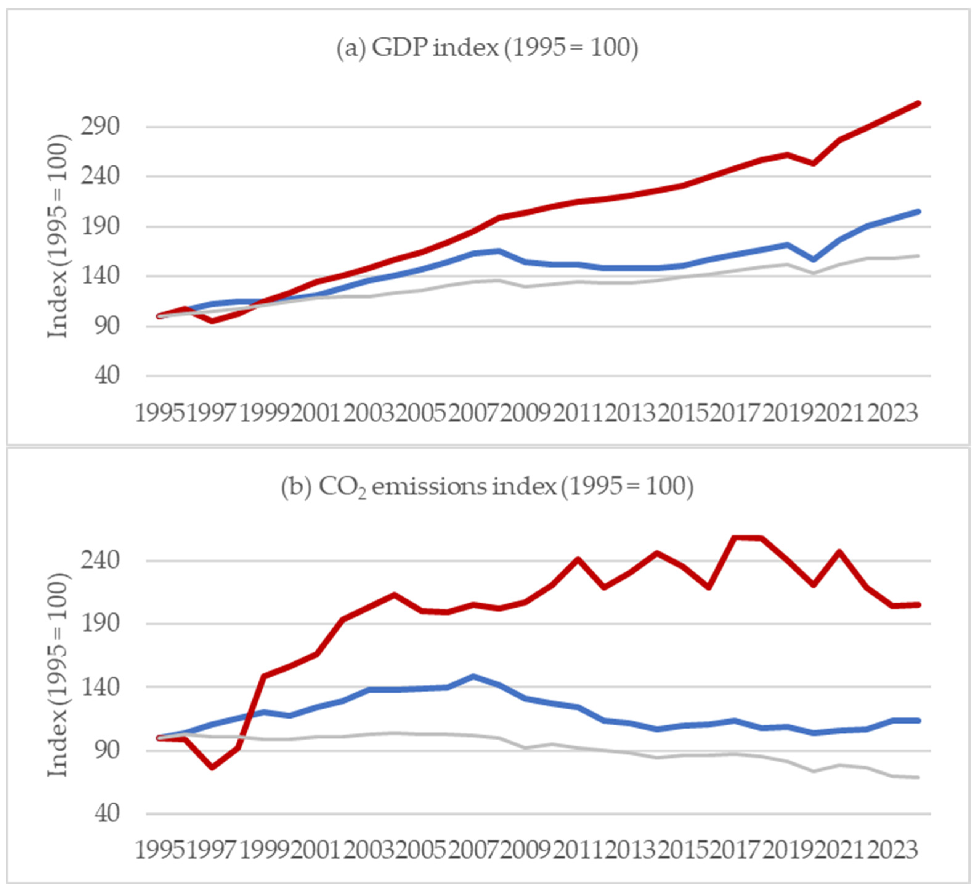
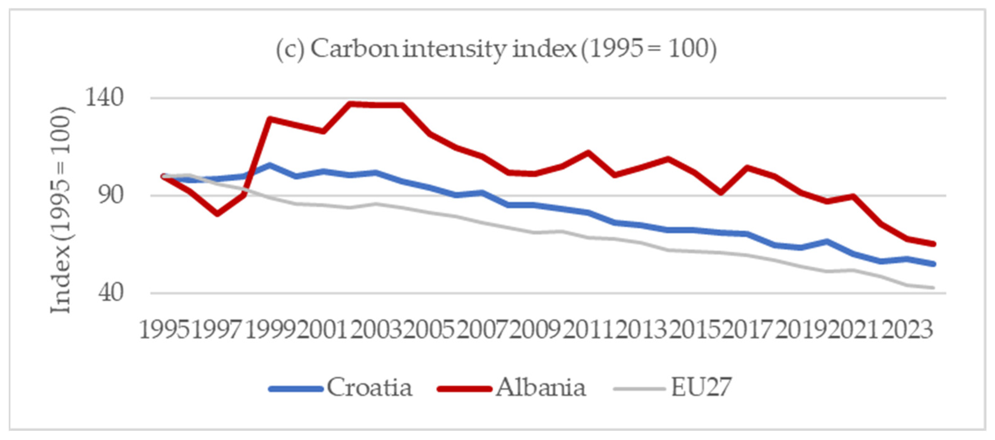
Figure 1 presents the indexed trajectories of real GDP, CO2 emissions, and carbon intensity in Croatia, Albania, and the EU27 over the period 1995–2024. All three series are expressed relative to their 1995 values to make changes over time comparable across economies.
Real GDP increased substantially in all three economies, although the trajectories differed (Figure 1a). Albania recorded the largest relative increase, with real GDP in 2024 exceeding three times its 1995 level. Croatia’s GDP approximately doubled over the same period, but its growth path included a prolonged downturn after the global financial crisis and a sharp contraction during the COVID-19 pandemic. Growth in the EU27 was more moderate and comparatively stable.
The emissions trajectories were less uniform (Figure 1b). EU27 CO2 emissions declined over the longer term, particularly from the mid-2000s onwards, despite continued growth in real GDP. Croatian emissions increased during the earlier part of the period and peaked in the late 2000s before generally declining; by 2024, however, they remained approximately 13% above their 1995 level. Albania recorded the largest fluctuations in emissions. Its CO2 emissions were more than twice their 1995 level by 2024, but the increase was interrupted by several periods of decline.
Carbon intensity declined over the full period in all three cases (Figure 1c). The EU27 shows the smoothest downward trajectory, while the Croatian series displays somewhat greater variation. Albania’s carbon intensity fluctuated more strongly, particularly in the earlier part of the period, but also ended substantially below its 1995 level. These trajectories show that lower carbon intensity can coexist with quite different developments in total emissions.
The long-term carbon intensity trends were assessed using the Mann–Kendall and Sen’s slope procedures described in Section 3.2. Because positive serial autocorrelation was identified in all three series, the TFPW-adjusted results are reported together with the Hamed–Rao robustness test and additional trend diagnostics in Table 2.
The trend tests confirm a statistically significant decline in carbon intensity in all three economies. The TFPW-adjusted Mann–Kendall results show negative and statistically significant trends for Croatia (τ = −0.906), Albania (τ = −0.704), and the EU27 (τ = −0.980), with p < 0.001 in each case. The stronger negative Kendall coefficients for the EU27 and Croatia indicate more consistent monotonic declines than in Albania, which is consistent with the greater variation visible in the Albanian series in Figure 1.
Sen’s slope is negative in all three cases. In absolute terms, the estimated annual decline in carbon intensity is −0.00940 for Croatia, −0.00727 for Albania, and −0.00692 for the EU27. The corresponding 95% confidence intervals remain entirely below zero. Since absolute slopes are affected by differences in carbon intensity levels, the relative estimates provide a more comparable measure of the pace of decline. Relative to mean carbon intensity, the estimated annual reductions are 2.33% for Croatia, 1.68% for Albania, and 2.64% for the EU27.
Positive Lag-1 autocorrelation is present in all three carbon intensity series. The Hamed–Rao modified Mann–Kendall test nevertheless remains statistically significant at p < 0.001 in each case, confirming that the conclusion of a long-term decline in carbon intensity is robust to the alternative treatment of serial dependence.
The trend results establish a broad long-term improvement in carbon intensity, but they do not show how consistently GDP growth and CO2 emissions were decoupled from one year to the next. The annual Tapio results presented in Section 4.2 examine this distinction more directly.

4.2. Annual Decoupling Patterns

Table 3 summarizes the distribution of annual Tapio decoupling states in Croatia, Albania, and the EU27 over the period 1996–2024. Detailed annual decoupling results are provided in Appendix A (Table A1).
The annual Tapio results show clear differences in the distribution of decoupling states across the three economies. Favorable decoupling, defined as the combined occurrence of strong and weak decoupling, was observed in 13 of 29 annual observations in Croatia (44.8%), 16 in Albania (55.2%), and 20 in the EU27 (69.0%). The composition of these favorable outcomes also differed. In Croatia, weak decoupling was more frequent than strong decoupling, accounting for 31.0% and 13.8% of annual observations, respectively. In Albania, strong decoupling accounted for 37.9% of observations and weak decoupling for 17.2%. The EU27 recorded the highest share of strong decoupling, at 48.3%, while weak decoupling accounted for a further 20.7%.
The remaining annual observations show greater variation in Croatia and Albania than in the EU27. Croatia recorded all eight Tapio states during the study period, including recessive decoupling in 17.2% of observations and expansive negative decoupling in 13.8%. In Albania, expansive negative decoupling accounted for 31.0% of annual observations, making it the second most frequent state after strong decoupling. In the EU27, expansive negative decoupling represented 10.3% of observations and recessive decoupling 13.8%, while strong negative decoupling, weak negative decoupling, and recessive coupling were not observed.
Although the favorable decoupling share was descriptively highest in the EU27 and lowest in Croatia, the differences were not statistically significant at the 5% level. The omnibus chi-square test did not indicate a statistically significant overall difference in favorable decoupling proportions across the three economies (χ2(2) = 3.458, p = 0.177). Pairwise two-proportion tests led to the same conclusion: EU27 versus Croatia (p = 0.063), EU27 versus Albania (p = 0.279), and Albania versus Croatia (p = 0.431). The observed differences in favorable annual decoupling frequencies should therefore be interpreted as descriptive rather than as statistically established differences between the economies.
Annual frequencies show how often favorable decoupling occurred, but they do not indicate whether the same pattern was maintained over longer intervals. This distinction is particularly relevant for Albania, where favorable decoupling occurred in more than half of the annual observations, while expansive negative decoupling was also relatively frequent. The medium-term analysis in the following section examines whether the annual patterns remain evident over longer time horizons.

4.3. Medium-Term Decoupling Patterns

Annual decoupling classifications may be sensitive to short-term changes in economic activity and emissions. To examine the growth–emissions relationship over a longer horizon, Table 4 reports Tapio decoupling results for contiguous medium-term intervals. The analysis uses consecutive endpoints from 1995 to 2020, followed by the final 2020–2024 interval reflecting the end of the available data series. Detailed calculations underlying the results reported in Table 4 are provided in Appendix B (Table A2).
The EU27 recorded favorable decoupling in all six contiguous intervals, comprising five strong-decoupling episodes and one weak-decoupling episode. This indicates a comparatively consistent medium-term growth–emissions pattern across the fixed intervals.
Croatia shows a more varied medium-term pattern, moving from coupling in the earlier part of the period toward predominantly favorable decoupling states thereafter. Four of the six contiguous intervals are classified as favorable, although the form of decoupling varies across periods and includes a recession-related episode in 2010–2015.
Albania also shows a shift toward more favorable medium-term outcomes. The earlier intervals are characterized by expansive negative decoupling or coupling, followed by weak decoupling and, from 2015 onward, strong decoupling. Overall, four of the six contiguous intervals are classified as favorable.
Compared with the annual results, the contiguous-period analysis provides a different view of temporal consistency. The EU27 maintains favorable decoupling across all six medium-term intervals, whereas Croatia and Albania move between different Tapio states. At the same time, the later intervals are more favorable in both national cases. Since results based on fixed intervals may depend on the choice of endpoints, the analysis was extended to rolling five-year windows. Each window shifts forward by one year, providing 25 overlapping windows from 1995–2000 to 2019–2024. Table 5 summarizes the resulting Tapio classifications, while the complete results for all 25 rolling windows are reported in Appendix C (Table A3).
The rolling-window results show a clear difference in the temporal consistency of medium-term decoupling across the three cases. The EU27 recorded favorable decoupling in 23 of the 25 rolling windows (92.0%), including strong decoupling in 18 windows (72.0%). Only two windows were classified in other Tapio states. The favorable medium-term pattern observed for the EU27 is therefore not limited to the fixed endpoints used in Table 4.
Croatia recorded favorable decoupling in 16 of the 25 rolling windows (64.0%). Weak decoupling was observed in nine windows (36.0%) and strong decoupling in seven (28.0%), while the remaining nine windows (36.0%) were classified in other Tapio states. Albania recorded favorable decoupling in 14 windows (56.0%), comprising eight strong-decoupling and six weak-decoupling windows. Other states accounted for 11 windows (44.0%), indicating greater variation across medium-term windows than in Croatia or the EU27.
The rolling results add an important qualification to the annual findings. Favorable annual decoupling occurred in 44.8% of observations in Croatia, 55.2% in Albania, and 69.0% in the EU27, whereas the corresponding shares across rolling five-year windows were 64.0%, 56.0%, and 92.0%. The descriptive ordering of Croatia and Albania differs across the two horizons: Croatia has the lower favorable share in the annual analysis but the higher share across rolling five-year windows. Annual decoupling frequency therefore does not fully describe how the growth–emissions relationship develops over medium-term horizons.
The contiguous and rolling results also differ in the degree of stability they reveal. The EU27 maintains favorable decoupling across all six contiguous intervals and 92.0% of rolling windows. Croatia and Albania show greater variation when the endpoints are shifted. These results are interpreted as evidence of the temporal consistency of medium-term decoupling rather than as a formal test of persistence.

4.4. Robustness and Sensitivity Analysis

The sensitivity of the Tapio results to the choice of classification thresholds was examined using alternative threshold pairs of 0.9/1.1 and 0.7/1.3, in addition to the baseline specification of 0.8/1.2. The detailed results are reported in Appendix D (Table A4).
The EU27 results are highly stable across the alternative specifications. Its favorable annual decoupling share changes only from 69.0% under the baseline specification to 72.4% under the 0.9/1.1 thresholds and remains at 69.0% under the 0.7/1.3 thresholds. More importantly, for the medium-term analysis, the favorable share remains unchanged at 92.0% across all three threshold specifications.
Croatia also shows relatively limited sensitivity to the choice of thresholds. Its favorable annual share ranges from 44.8% to 51.7%, while the rolling five-year share ranges from 60.0% to 64.0%. Albania is more sensitive, particularly in the rolling analysis: its favorable share changes from 56.0% under the baseline specification to 68.0% with the 0.9/1.1 thresholds and 52.0% with the 0.7/1.3 thresholds. The annual Albanian share varies within a narrower range, from 48.3% to 55.2%.
The threshold sensitivity analysis therefore leaves the main comparative pattern largely unchanged. The EU27 retains the highest favorable decoupling share under every specification, particularly across rolling five-year windows. Croatia’s results are comparatively stable, whereas Albania’s medium-term classification is more sensitive to the precise threshold choice.
A second sensitivity check addresses cases in which the Tapio index may become unusually large because the change in GDP is close to zero. Observations with an absolute GDP change below 0.5% were therefore identified and excluded in an alternative specification. The identified observations and the resulting favorable decoupling shares are reported in Appendix E (Table A5 and Table A6).
Four annual observations met the near-zero GDP criterion: 2011 and 2013 for Croatia and 2013 and 2023 for the EU27. In the rolling five-year analysis, only the EU27 window for 2007–2012 met the criterion. No annual or rolling observations were identified for Albania. Excluding these observations produced only minor changes in the favorable decoupling shares: Croatia’s annual share increased from 44.8% to 48.1%, while the EU27 annual and rolling shares increased slightly. Croatia’s rolling result remained unchanged, and Albania’s results were unaffected because no observations met the exclusion criterion.
The near-zero GDP sensitivity check therefore does not materially alter the baseline results. Taken together, the alternative-threshold and near-zero GDP analyses show that the main comparative pattern is broadly maintained across the robustness specifications, although Albania’s rolling results are more sensitive to the choice of Tapio thresholds.
A further sensitivity check excluded the 2020 and 2021 annual observations to assess the influence of the COVID-19 contraction and subsequent recovery. The favorable annual decoupling share changed only marginally for Croatia, from 44.8% (13/29) to 44.4% (12/27), while it increased to 59.3% (16/27) for Albania and 74.1% (20/27) for the EU27. The descriptive ordering therefore remained unchanged, with the EU27 showing the highest favorable share, followed by Albania and Croatia.
As an additional robustness check, the main analyses were recalculated using EEA/UNFCCC CO2 emissions data in place of the baseline WDI emissions series while retaining the same GDP series. This specification assesses whether the principal findings are sensitive to the choice of emissions data source. Table 6 compares the baseline and alternative-source results.
The alternative emissions data produce very similar results for Croatia and the EU27. Croatia’s favorable annual, rolling, and contiguous results are unchanged, while the EU27 shows only a small increase in the favorable annual share; its medium-term results remain unchanged. The relative Sen slopes are also similar across the two emissions sources.
Albania shows greater sensitivity to the emissions source in the annual results. Its favorable annual share decreases from 55.2% with WDI data to 44.8% with EEA data, while the relative Sen slope changes from −1.68% to −1.01% per year. The medium-term results, however, remain unchanged at the aggregate level: favorable decoupling occurs in 56.0% of the rolling five-year windows and in four of the six contiguous intervals under both data sources. Overall, the alternative emissions data leave the main medium-term comparative pattern unchanged, while showing that some annual results, particularly for Albania, are more sensitive to the choice of emissions source.
As a further robustness check, production-based and consumption-based CO2 emissions were compared for Croatia over the common 2010–2023 period (Appendix F, Table A7). Real GDP increased by 29.4% over this period, while production-based CO2 emissions declined by 10.9% and consumption-based emissions by 5.4%. The corresponding decline in carbon intensity was 31.1% and 26.9%, respectively. Favorable annual Tapio outcomes were somewhat less frequent under consumption-based accounting (4/13; 30.8%) than under production-based accounting (5/13; 38.5%). Thus, the consumption-based specification gives a somewhat less favorable assessment, but the favorable decoupling evidence does not disappear when emissions embodied in international trade are taken into account.

4.5. LMDI Decomposition of Energy Sector CO2 Emissions

To examine the factors associated with changes in energy sector CO2 emissions, Table 7 reports the LMDI decomposition for 1995–2024. The analysis separates the total change into activity, energy intensity, and carbon-intensity-of-energy effects.
The decomposition shows that economic activity exerted upward pressure on energy sector CO2 emissions in all three cases. In the EU27, this effect was more than offset by lower energy intensity and lower carbon intensity of energy, resulting in a substantial net emissions decline. In Croatia, the activity effect was largely offset by improved energy intensity and, to a lesser extent, lower carbon intensity of energy. In Albania, improved energy intensity partly offset the activity effect, whereas the carbon-intensity-of-energy effect was close to zero and slightly positive. A supplementary check for Albania found only a weak and statistically non-significant association between annual changes in hydropower generation and the annual carbon-intensity-of-energy effect (Pearson r = −0.12, p = 0.531), providing no clear evidence of a systematic annual relationship between the two.

4.6. CBAM Trade Exposure of Albania

To complement the decoupling analysis with a regulatory transition risk perspective, Albania’s trade exposure to products covered by the EU Carbon Border Adjustment Mechanism (CBAM) was examined over the period 2015–2024. Table 8 reports the annual share of CBAM-covered products in total EU27 imports from Albania and shows how this exposure is distributed across the six CBAM sectors.
During 2015–2020, CBAM-related trade exposure remained within a relatively narrow range, from 7.83% to 9.66% of total EU27 imports from Albania. A marked increase occurred thereafter, with exposure rising to 13.88% in 2021 and reaching a peak of 18.30% in 2022. It subsequently declined to 16.30% in 2023 and 14.02% in 2024. Despite the decline from the 2022 peak, exposure in 2024 remained above the range observed throughout 2015–2020.
The exposure was concentrated in three sectors: electricity, iron and steel, and aluminum. The marked increase in total exposure in 2021–2022 coincided with a substantial rise in the electricity component, which increased from 3.13% of total EU27 imports from Albania in 2020 to 4.48% in 2021 and 8.76% in 2022. Iron and steel also represented a substantial component, accounting for 6.08% in 2021 and 6.01% in 2022, while aluminum accounted for 2.83% and 3.19%, respectively. By 2024, electricity remained the largest individual component at 5.39%, followed by iron and steel at 4.89% and aluminum at 3.15%. Cement accounted for 0.58%, fertilizers remained below 0.01%, and no hydrogen imports were recorded.
Overall, Albania’s CBAM trade exposure increased relative to the pre-2021 period and remained concentrated in electricity, iron and steel, and aluminum. The indicator reflects regulatory trade exposure rather than the actual financial cost of CBAM compliance.

5. Discussion

5.1. Decoupling Performance and Temporal Consistency

The results point to a common long-term development across Croatia, Albania, and the EU27: economic growth has become less carbon-intensive over the period under study. Carbon intensity declined significantly in all three cases, with negative Sen slopes remaining statistically significant after accounting for serial autocorrelation. In relative terms, the decline was strongest for the EU27 (−2.64% per year), followed by Croatia (−2.33%) and Albania (−1.68%). This indicates a sustained improvement in emissions per unit of economic output but does not in itself imply absolute decoupling of economic growth from total CO2 emissions. This distinction is consistent with Shuai et al. (2019), who identify a sequential pattern in which decoupling from carbon intensity is more common than decoupling from per capita or total carbon emissions across 133 countries.
The baseline annual Tapio results provide a more differentiated picture. Strong or weak decoupling occurred in 69.0% of observations for the EU27, 55.2% for Albania, and 44.8% for Croatia. These differences are descriptive rather than statistically established: the omnibus test and all pairwise comparisons are non-significant at the 5% level. The relatively favorable EU27 pattern is nevertheless consistent with evidence of substantial decoupling progress across European economies (Cautisanu & Hatmanu, 2023; Ziemblińska et al., 2025). Bianco et al. (2024) similarly report strong decoupling for the EU27 and relate declining emissions to lower energy intensity and changes in the carbon intensity of energy supply. The LMDI results in the present study are consistent with this interpretation: the positive activity effect for the EU27 was more than offset by reductions in both energy intensity and the carbon intensity of energy. These are accounting contributions rather than causal estimates of individual technologies or policies. The LMDI results should therefore be interpreted as complementary evidence on energy-related drivers rather than as a decomposition of the total CO2 series underlying the Tapio analysis.
The distinction between annual and medium-term results becomes clearer when the two horizons are considered together. Under the baseline specification, the descriptive ordering differs across the two horizons: Albania has a higher favorable share in the annual observations (55.2% versus 44.8%), whereas Croatia has a higher favorable share across the rolling five-year windows (64.0% versus 56.0%). Croatia’s result suggests that relatively frequent unfavorable year-to-year movements can coexist with a more favorable cumulative growth–emissions relationship over multi-year horizons. The EU27 shows the highest favorable share at both horizons, reaching 69.0% annually and 92.0% across rolling windows. These results suggest that the frequency of favorable individual years does not necessarily provide the same comparative picture as the medium-term analysis. This feature would not be apparent from conventional annual Tapio classifications alone.
The contiguous and rolling-window results support the same interpretation without constituting a formal test of persistence. They indicate that decoupling assessments can change with the observation horizon and that favorable outcomes in individual years need not translate into equally consistent medium-term patterns. This is consistent with previous studies showing that decoupling outcomes vary across periods and analytical horizons (Cohen et al., 2022; Hubacek et al., 2021; Han et al., 2022; R. Xie et al., 2022), as well as with recent emphasis on the consistency of decoupling across time (Kilinc-Ata et al., 2026).
The robustness checks qualify this comparison further. The EU27 rolling result is highly stable across alternative Tapio thresholds, while Croatia shows only limited variation; Albania’s medium-term classification is more threshold-sensitive and should therefore be interpreted more cautiously. The alternative EEA emissions series also shows that Albania’s higher annual favorable share relative to Croatia is not source-robust, whereas the rolling-window ordering remains unchanged. The medium-term comparative pattern is therefore less sensitive to the choice of emissions source than the annual comparison. Although the study period includes the COVID-19 shock and subsequent energy market disruptions, the rolling-window analysis shows that the broader comparative pattern remains visible across alternative window placements.
Taken together, the results show why annual frequency and medium-term temporal consistency should not be treated as interchangeable measures of decoupling performance. Annual classifications capture short-term changes and reversals and may also be more sensitive to the emissions series used, whereas the medium-term analysis indicates whether a favorable relationship remains visible over broader and shifting time horizons. This distinction is particularly relevant for smaller economies, where year-to-year changes may be more exposed to economic and energy-related fluctuations.

5.2. Country-Specific and EU27 Patterns

The medium-term results suggest a gradual improvement in Croatia, although the path has not been uniform. The later contiguous intervals are more favorable than the earlier ones, and the rolling-window results indicate greater temporal consistency than the annual frequencies alone would suggest. This development coincides with changes in Croatia’s economic, energy, and institutional environment. Previous research points to improvements in energy efficiency and a growing role of renewable energy sources (Jeleč Raguž, 2026), while the European Environment Agency reports further growth in renewable energy production and declining energy consumption, alongside continuing challenges in transport and other emission-intensive activities (EEA, 2025b). Croatia’s accession to the EU in 2013 also brought the country more fully within the EU climate and energy policy framework. These developments provide relevant context, but the present analysis cannot determine how much of the observed change is attributable to EU integration, energy policy, technological change, shifts in economic structure, or other factors.
Aggregate results also conceal differences across economic activities. Recent evidence for Croatia shows that carbon intensity and decoupling patterns differ across tourism-related sectors and individual transport modes (Jeleč Raguž et al., 2026). The national results should therefore be read as the combined outcome of potentially different sectoral developments. The more favorable medium-term pattern does not imply that decarbonization has progressed evenly across the Croatian economy. Continued renewable-energy development, lower energy consumption, and the decarbonization of transport remain relevant areas for further progress (EEA, 2025b).
Albania presents a different pattern. Its carbon intensity has declined significantly, and favorable decoupling occurs in more than half of the annual observations, but expansive negative decoupling remains relatively frequent, and the rolling-window results are more sensitive to alternative Tapio thresholds. Evidence for the Western Balkans confirms the continuing importance of the relationship between economic activity, energy use, and CO2 emissions (Pejović et al., 2021; Zhigolli & Fetai, 2024). The LMDI results provide a more direct perspective for Albania: improved energy intensity partly offset the emissions increase associated with economic activity, while the carbon-intensity-of-energy effect was close to zero over the full period. Although Albania’s electricity system is strongly dependent on hydropower and exposed to hydrological conditions (EEA, 2025a), the supplementary annual check found no statistically significant association between changes in hydropower generation and the carbon-intensity-of-energy effect. The present evidence therefore does not support attributing Albania’s decoupling pattern primarily to hydropower fluctuations.
The comparison between Croatia and Albania should not, however, be reduced to a simple EU versus non-EU distinction. Previous studies report substantial decoupling progress within the EU but also considerable variation across countries and periods (Cautisanu & Hatmanu, 2023; Ziemblińska et al., 2025), while research on the Western Balkans points to continuing links between growth, energy use, and emissions (Pejović et al., 2021; Zhigolli & Fetai, 2024). The two countries differ in their institutional settings, economic structures, and energy systems, but the present analysis cannot identify EU membership itself as the source of their different trajectories.
The EU27 serves a different purpose in the comparison. Its decoupling pattern is more consistent across rolling windows and less sensitive to alternative Tapio thresholds, in line with broader evidence of decarbonization progress in the EU (Bianco et al., 2024; Cautisanu & Hatmanu, 2023). However, the EU27 is an aggregate of economies with different structures, energy systems, and emission trajectories, whereas Croatia and Albania are individual countries. Aggregation can smooth country-specific shocks and offset divergent national developments. The EU27 should therefore be interpreted as a reference trajectory rather than as a directly comparable unit against which Croatia and Albania can be ranked.

5.3. CBAM Exposure and Transition Risk Implications for Albania

The CBAM analysis adds a trade-related transition risk dimension to the decoupling results for Albania. Exposure increased markedly after 2020 and remained concentrated in electricity, iron and steel, and aluminum. The increase in 2021–2022 was particularly pronounced in electricity, whose share rose from 3.13% of total EU27 imports from Albania in 2020 to 4.48% in 2021 and 8.76% in 2022. This period coincided with the sharp increase in European electricity prices during the energy crisis. The European Power Benchmark averaged EUR 230/MWh in 2022, 121% above its 2021 level (European Commission, 2023). Part of the increase in the value-based CBAM exposure indicator may therefore reflect higher electricity prices and changes in trade values rather than a proportional increase in the underlying carbon exposure of Albanian production.
The sectoral concentration of exposure is relevant because CBAM applies to carbon-intensive imports in sectors where differences in carbon pricing may create a risk of carbon leakage (European Parliament & Council of the European Union, 2023). It is also informative when considered together with the LMDI results. For Albania, the carbon-intensity-of-energy effect over 1995–2024 was close to zero, while electricity remained the largest individual component of CBAM trade exposure in 2024. Taken together, these results suggest that a near-term reduction in Albania’s CBAM-related exposure is unlikely to come primarily from improvements in the carbon intensity of electricity generation. The transition risk channel identified here therefore depends on both the composition of exports and the carbon characteristics of the activities producing them.
The indicator itself remains a measure of trade exposure rather than financial CBAM risk. Translating it into a monetary risk measure would require product-level embedded emissions per unit of covered exports and an applicable path for CBAM certificate prices, together with any carbon price effectively paid in the country of origin. Combining these elements with the physical quantities and trade values of covered products would provide a direct next step from the present trade exposure measure towards an estimate of carbon cost exposure. Such an estimate would still need to distinguish indicative exposure from the actual liability of individual firms.
For firms and policymakers, the concentration of Albania’s CBAM exposure in a small number of sectors has practical implications. Electricity, iron and steel, and aluminum account for most of the country’s CBAM-covered trade, making emissions monitoring and the carbon performance of these activities increasingly relevant to competitiveness in the EU market. Similar concerns have been raised for the Western Balkans more broadly, where the economic implications of CBAM differ considerably across carbon-intensive sectors (Vućemilović Grgić & Knežević Mužić, 2026). The results reported here do not imply that Albania’s exposure will translate directly into changes in exports, profitability, investment, or financing. Assessing such effects would require firm-level evidence on CBAM-related costs and on the ability of producers and importers to reduce, absorb, or pass through those costs.

5.4. Limitations and Future Research

Several limitations should be considered when interpreting the results. First, the core analysis uses aggregate national GDP and production-based CO2 emissions. This provides a consistent basis for comparing economy-wide decoupling patterns, but it does not capture sectoral differences or firm-level heterogeneity. A supplementary consumption-based check for Croatia partly addresses emissions embodied in international trade, but it is limited to 2010–2023 and could not be replicated for Albania because a comparable consumption-based CO2 series is not available in the FIGARO dataset. It therefore does not replace the production-based framework used in the main cross-country analysis. The results should not be interpreted as evidence of uniform decarbonization across economic activities. Future research could extend the analysis using longer consumption-based series and sectoral data.
Second, Tapio classifications remain sensitive to the observation horizon, selected endpoints, and elasticity thresholds. The use of multiple time horizons and sensitivity checks reduces reliance on any single specification but does not eliminate this dependence. The five-year results should therefore be interpreted as evidence of medium-term temporal consistency rather than as a formal statistical test of persistence. Exceptional events such as the COVID-19 shock and energy market disruptions may also affect individual classifications, while comparison with the EU27 is subject to the smoothing effects inherent in an aggregate benchmark.
Finally, the CBAM indicator measures Albania’s trade exposure to covered product groups, not the financial risk associated with that exposure. A monetary measure would require product-level physical trade quantities and embedded-emissions intensities, combined with an applicable path for CBAM certificate prices and information on carbon prices effectively paid in the country of origin. Future research could combine these elements with firm-level data to examine how CBAM-related costs affect profitability, investment, financing, and export performance.

6. Conclusions

This study shows that declining carbon intensity and favorable decoupling should not be treated as equivalent indicators of progress towards a low-carbon economy. Although carbon intensity declined significantly in Croatia, Albania, and the EU27, the annual and medium-term results reveal different degrees of temporal consistency in the relationship between economic growth and CO2 emissions. The annual results do not establish statistically significant differences in favorable decoupling frequencies between the cases, while the rolling-window results are descriptive because the windows overlap. The comparison nevertheless shows that conclusions about decoupling can differ across time horizons, with the annual results also being more sensitive to the choice of emissions data source. Evidence of medium-term favorable decoupling is also less classification-robust for Albania than for Croatia and the EU27, as Albania’s rolling-window results are more sensitive to alternative Tapio thresholds. The EU27 provides a more consistent reference trajectory, although its aggregate nature limits direct comparison with individual economies.
For smaller transition economies, these findings highlight the value of assessing decoupling across more than one time horizon and alongside regulatory pressures linked to the low-carbon transition. The CBAM results for Albania show that declining carbon intensity and favorable decoupling can coexist with continued trade exposure to EU carbon regulation. This exposure reflects the composition of Albania’s exports and is therefore distinct from the domestic growth–emissions relationship measured by the decoupling indicators. The findings also show why favorable annual outcomes alone provide an incomplete picture: the assessment can change when the growth–emissions relationship is examined over a medium-term horizon.

Author Contributions

Conceptualization, M.J.R.; methodology, M.J.R., E.P.B. and A.E.; software and formal analysis, M.J.R., E.P.B. and A.E.; investigation, M.J.R., E.P.B. and A.E.; data curation, M.J.R., E.P.B. and A.E.; writing—original draft preparation, M.J.R.; writing—review and editing, M.J.R., E.P.B. and A.E.; visualization, M.J.R., E.P.B. and A.E. All authors have read and agreed to the published version of the manuscript.

Funding

This research was funded by the Faculty of Tourism and Rural Development in Požega, Josip Juraj Strossmayer University of Osijek, Croatia.

Institutional Review Board Statement

Not applicable.

Informed Consent Statement

Not applicable.

Data Availability Statement

The original data presented in the study are openly available in the World Bank World Development Indicators at https://data.worldbank.org/indicator/ (accessed on 1 September 2026), the European Environment Agency Greenhouse Gases Data Viewer at https://www.eea.europa.eu/data-and-maps/data/data-viewers/greenhouse-gases-viewer (accessed on 1 September 2026), and Eurostat datasets (including Energy Balances, FIGARO CO2 Emission Footprints, and Comext Trade Data) at https://ec.europa.eu/eurostat/web/main/data/database (accessed on 1 September 2026).

Acknowledgments

The authors would like to thank the editors and the anonymous reviewers for their valuable comments and suggestions. During the preparation of this manuscript, ChatGPT (GPT-5.6 Sol, OpenAI) was used to assist with translating selected sections into English, improving the language and readability of the text, drafting the abstract, and checking selected calculations and formulations during the revision process. All analyses, interpretations, and conclusions were developed by the authors. The authors reviewed all AI-assisted text and take full responsibility for the content of this publication.

Conflicts of Interest

The authors declare no conflicts of interest.

Abbreviations

The following abbreviations are used in this manuscript:
AbbreviationDefinition
CBAMEU Carbon Border Adjustment Mechanism
CICarbon intensity
CO2Carbon dioxide
DITapio decoupling elasticity
ECExpansive coupling
EKCEnvironmental Kuznets Curve
ENDExpansive negative decoupling
EUEuropean Union
EU27European Union (27 Member States)
GDPGross domestic product
LMDILogarithmic Mean Divisia Index
MKMann–Kendall test
OECDOrganization for Economic Co-operation and Development
RCRecessive coupling
RDRecessive decoupling
SDStrong decoupling
SNDStrong negative decoupling
TFPWTrend-Free Pre-Whitening Procedure
WDWeak decoupling
WDIWorld Development Indicators
WNDWeak negative decoupling

Appendix A. Annual Tapio Classifications

Appendix A provides the detailed annual Tapio elasticity and decoupling classification results summarized in Table 3.
Table A1. Annual Tapio elasticity and decoupling classification by country (1996–2024).
YearTapio ElasticityDecoupling StateTapio ElasticityDecoupling StateTapio ElasticityDecoupling State
CroatiaAlbaniaEU27
19960.697WD−0.099SD1.452END
19971.043EC1.972RD−0.723SD
19981.739END2.545END−0.071SD
1999−5.639SND4.996END−0.599SD
2000−0.954SD0.634WD0.124WD
20011.933END0.721WD0.678WD
20020.684WD3.562END−0.260SD
20031.168EC0.959EC2.938END
2004−0.022SD0.914EC0.076WD
20050.125WD−1.172SD−0.300SD
20060.160WD−0.055SD0.124WD
20071.263END0.413WD−0.321SD
2008−2.448SD−0.174SD−3.918SD
20091.038RC0.785WD1.782RD
20102.530RD2.225END1.502END
201120.943RD3.855END−1.440SD
20123.642RD−9.392SD2.592RD
201316.166RD2.992END78.827RD
20146.869RD3.106END−2.731SD
20150.847EC−1.994SD0.839EC
20160.400WD−1.770SD0.133WD
20170.871EC5.524END0.284WD
2018−1.884SD−0.138SD−1.037SD
20190.374WD−3.182SD−2.453SD
20200.523WND2.521RD1.664RD
20210.145WD1.329END1.069EC
20220.100WD−2.384SD−0.694SD
20231.552END−1.659SD−19.136SD
20240.021WD0.124WD−1.771SD
Note: DI = Decoupling Index; SD = strong decoupling; WD = weak decoupling; EC = expansive coupling; END = expansive negative decoupling; SND = strong negative decoupling; WND = weak negative decoupling; RC = recessive coupling; RD = recessive decoupling. Decoupling states are classified according to the eight-category Tapio (2005) framework presented in Table 1, taking into account both the direction of annual changes in GDP and CO2 emissions and the value of the DI. Extreme DI values may occur when annual GDP growth is close to zero; therefore, isolated extreme coefficients should be interpreted with caution, with greater emphasis placed on the corresponding decoupling state than on their absolute magnitude. Source: Authors’ calculations based on World Bank (2026a, 2026b).

Appendix B. Contiguous Five-Year Calculations/Raw Endpoints

Appendix B provides the detailed calculations underlying the medium-term Tapio decoupling results reported in Table 4.
Table A2. Detailed calculation of medium-term Tapio decoupling indices in Croatia, Albania, and the EU27, 1995–2024.
EconomyPeriodGDP Start (bn)GDP End (bn)ΔGDP (%)CO2 Start (Mt)CO2 End (Mt)ΔCO2 (%)DIDecoupling State
Croatia1995–200033.74839.68017.57716.501519.378017.4320.992EC
2000–200539.68049.66525.16419.378022.850717.9210.712WD
2005–201049.66551.3953.48322.850720.9405−8.359−2.400SD
2010–201551.39550.999−0.77020.940518.0245−13.92518.077RD
2015–202050.99953.0203.96318.024517.1915−4.621−1.166SD
2020–202453.02069.02830.19317.191518.67968.6560.287WD
Albania1995–20004.9706.15323.8132.07023.232956.1642.359END
2000–20056.1538.17032.7753.23294.148928.3340.864EC
2005–20108.17010.42827.6434.14894.567010.0770.365WD
2010–201510.42811.4709.9934.56704.87566.7570.676WD
2015–202011.47012.5939.7934.87564.5676−6.317−0.645SD
2020–202412.59315.56823.6234.56764.2437−7.091−0.300SD
EU271995–20009811.29011,319.87015.3763586.69183559.5714−0.756−0.049SD
2000–200511,319.87012,347.9809.0823559.57143685.78283.5460.390WD
2005–201012,347.98012,976.5945.0913685.78283409.4609−7.497−1.473SD
2010–201512,976.59413,656.2535.2383409.46093082.0529−9.603−1.833SD
2015–202013,656.25314,047.4042.8643082.05292638.4092−14.394−5.026SD
2020–202414,047.40415,711.33011.8452638.40922462.3895−6.671−0.563SD
Note: DI = decoupling index; SD = strong decoupling; WD = weak decoupling; EC = expansive coupling; END = expansive negative decoupling; RD = recessive decoupling. GDP is expressed in billion constant 2015 US$, while CO2 emissions are expressed in Mt CO2e. Percentage changes and Tapio decoupling indices were calculated using the original unrounded data; GDP and CO2 values displayed in the table are rounded for presentation. Relative changes are calculated between the start and end years of each contiguous interval as (Xend − Xstart)/Xstart × 100. The Tapio decoupling index is calculated as DI = %ΔCO2/%ΔGDP. Decoupling states are classified according to the eight-category Tapio (2005) framework presented in Table 1. The final interval covers 2020–2024 because the available data series ends in 2024. Source: Authors’ calculations based on World Bank (2026a, 2026b).

Appendix C. Rolling Five-Year Decoupling Classifications

Appendix C provides the complete rolling five-year Tapio decoupling classifications underlying the summary results reported in Table 5.
Table A3. Rolling five-year Tapio decoupling classifications, 1995–2024.
PeriodCroatia DICroatia StateAlbania DIAlbania StateEU27 DIEU27 State
1995–20000.992EC2.359END−0.049SD
1996–20011.362END2.634END−0.129SD
1997–20021.201END3.144END−0.027SD
1998–20031.114EC2.682END0.223WD
1999–20040.595WD1.204END0.418WD
2000–20050.712WD0.864EC0.390WD
2001–20060.441WD0.690WD0.236WD
2002–20070.553WD0.189WD0.137WD
2003–20080.113WD−0.012SD−0.270SD
2004–2009−0.493SD−0.098SD−2.244SD
2005–2010−2.400SD0.365WD−1.473SD
2006–20116.926RD0.896EC−3.036SD
2007–20122.764RD0.406WD24.854RD
2008–20132.050RD1.215END10.481RD
2009–20144.272RD1.770END−1.679SD
2010–201518.077RD0.676WD−1.833SD
2011–2016−3.828SD−0.801SD−1.297SD
2012–20170.006WD1.287END−0.455SD
2013–2018−0.281SD0.726WD−0.321SD
2014–20190.104WD−0.144SD−0.326SD
2015–2020−1.166SD−0.645SD−5.026SD
2016–2021−0.319SD0.835EC−1.194SD
2017–2022−0.352SD−0.926SD−1.444SD
2018–20230.273WD−1.208SD−2.740SD
2019–20240.203WD−0.761SD−2.736SD
Note: DI = decoupling index; SD = strong decoupling; WD = weak decoupling; EC = expansive coupling; END = expansive negative decoupling; RD = recessive decoupling. Rolling changes are calculated between endpoints separated by five years. Baseline Tapio thresholds of 0.8 and 1.2 are applied. Source: Authors’ calculations based on World Bank (2026a, 2026b), World Development Indicators.

Appendix D. Threshold Sensitivity

Appendix D provides the detailed threshold sensitivity results underlying the robustness analysis reported in Section 4.4.
Table A4. Sensitivity of favorable decoupling shares to alternative Tapio thresholds.
FrequencyEconomy0.8/1.2 (Baseline)0.9/1.10.7/1.3
AnnualCroatia44.8%51.7%44.8%
AnnualAlbania55.2%55.2%48.3%
AnnualEU2769.0%72.4%69.0%
Rolling 5-yearCroatia64.0%64.0%60.0%
Rolling 5-yearAlbania56.0%68.0%52.0%
Rolling 5-yearEU2792.0%92.0%92.0%
Note: Favorable decoupling comprises strong and weak decoupling. The baseline specification applies Tapio thresholds of 0.8 and 1.2; robustness is assessed using alternative threshold pairs of 0.9/1.1 and 0.7/1.3. Annual percentages are based on 29 observations per economy and rolling percentages on 25 five-year windows. Source: Authors’ calculations based on World Bank (2026a, 2026b).

Appendix E. Near-Zero GDP Sensitivity

Appendix E provides the detailed near-zero GDP sensitivity results underlying the robustness analysis reported in Section 4.4.
Table A5. Observations identified by the near-zero GDP sensitivity criterion.
FrequencyEconomyYear/PeriodΔGDP (%)DIBaseline State
AnnualCroatia2011−0.11120.943RD
AnnualCroatia2013−0.13416.166RD
AnnualEU272013−0.03378.827RD
AnnualEU2720230.454−19.136SD
Rolling 5-yearEU272007–2012−0.45824.854RD
Note: DI = decoupling index; RD = recessive decoupling; SD = strong decoupling. Observations are flagged when the absolute change in GDP is below 0.5%, i.e., |ΔGDP| < 0.5%. Such observations may generate unusually large absolute DI values because the denominator of the Tapio index approaches zero. Albania had no annual or rolling five-year observations satisfying this criterion. Source: Authors’ calculations based on World Bank (2026a, 2026b).
Table A6. Sensitivity of favorable decoupling shares to the exclusion of near-zero GDP observations.
FrequencyEconomyBaselineExcluding |ΔGDP| < 0.5%
AnnualCroatia44.8% (13/29)48.1% (13/27)
AnnualAlbania55.2% (16/29)55.2% (16/29)
AnnualEU2769.0% (20/29)70.4% (19/27)
Rolling 5-yearCroatia64.0% (16/25)64.0% (16/25)
Rolling 5-yearAlbania56.0% (14/25)56.0% (14/25)
Rolling 5-yearEU2792.0% (23/25)95.8% (23/24)
Note: Favorable decoupling comprises strong decoupling (SD) and weak decoupling (WD). The sensitivity specification excludes observations for which the absolute change in GDP is below 0.5% (|ΔGDP| < 0.5%). Baseline observations are retained in the primary analysis, while their exclusion is used only as a robustness check. Source: Authors’ calculations based on World Bank (2026a, 2026b).

Appendix F. Consumption-Based Emissions Robustness Check

Appendix F reports the supplementary robustness check comparing production-based and consumption-based CO2 outcomes for Croatia over their common 2010–2023 period.
Table A7. Consumption-based robustness check for Croatia, 2010–2023.
IndicatorProduction-Based CO2Consumption-Based CO2
CO2 change, 2010–2023 (%)−10.9−5.4
Real GDP change, 2010–2023 (%)+29.4+29.4
Carbon intensity change, 2010–2023 (%)−31.1−26.9
Favorable annual Tapio outcomes5/13 (38.5%)4/13 (30.8%)
Note: Favorable decoupling comprises strong and weak decoupling. Production-based CO2 corresponds to the World Bank WDI series used in the main analysis. Consumption-based CO2 refers to Eurostat FIGARO carbon dioxide emission footprints for Croatia, including all countries of origin and all NACE activities plus households. The comparison is restricted to 2010–2023 because of the availability of the consumption-based series. Source: Authors’ calculations based on World Bank (2026a, 2026b) and Eurostat (2026a).

References

  1. Ahmad, N., Du, L., Lu, J., Wang, J., Li, H.-Z., & Hashmi, M. Z. (2017). Modelling the CO2 emissions and economic growth in Croatia: Is there any environmental Kuznets curve? Energy, 123, 164–172. [Google Scholar] [CrossRef] [Scilit]
  2. Ang, B. W. (2005). The LMDI approach to decomposition analysis: A practical guide. Energy Policy, 33(7), 867–871. [Google Scholar] [CrossRef] [Scilit]
  3. Bianco, V., Cascetta, F., & Nardini, S. (2024). Analysis of the carbon emissions trend in European Union. A decomposition and decoupling approach. Science of the Total Environment, 909, 168528. [Google Scholar] [CrossRef] [Scilit] [PubMed]
  4. Brizga, J., Feng, K., & Hubacek, K. (2014). Drivers of greenhouse gas emissions in the Baltic States: A structural decomposition analysis. Ecological Economics, 98, 22–28. [Google Scholar] [CrossRef] [Scilit]
  5. Cautisanu, C., & Hatmanu, M. (2023). A study of the decoupling of economic growth from CO2 and HFCs emissions in the EU27 countries. Energies, 16(14), 5546. [Google Scholar] [CrossRef] [Scilit]
  6. Cohen, G., Jalles, J. T., Loungani, P., & Pizzuto, P. (2022). Trends and cycles in CO2 emissions and incomes: Cross-country evidence on decoupling. Journal of Macroeconomics, 71, 103397. [Google Scholar] [CrossRef] [Scilit]
  7. Dinda, S. (2004). Environmental Kuznets Curve hypothesis: A survey. Ecological Economics, 49(4), 431–455. [Google Scholar] [CrossRef] [Scilit]
  8. European Commission. (2019). Communication from the commission to the European parliament, the European council, the council, the European economic and social committee and the committee of the regions: The European green deal (COM(2019) 640 final). Available online: https://eur-lex.europa.eu/legal-content/EN/TXT/?uri=CELEX:52019DC0640 (accessed on 1 August 2026).
  9. European Commission. (2023). Quarterly reports confirm stabilising gas and electricity markets at the end of 2022. Available online: https://energy.ec.europa.eu/news/quarterly-reports-confirm-stabilising-gas-and-electricity-markets-end-2022-2023-05-17_en (accessed on 11 September 2026).
  10. European Environment Agency (EEA). (2025a). Albania: Country profile—Europe’s environment 2025. Available online: https://www.eea.europa.eu/en/europe-environment-2025/countries/albania (accessed on 10 August 2026).
  11. European Environment Agency (EEA). (2025b). Croatia: Country profile—Europe’s environment 2025. Available online: https://www.eea.europa.eu/en/europe-environment-2025/countries/croatia (accessed on 10 August 2026).
  12. European Environment Agency (EEA). (2026). EEA greenhouse gases—Data viewer. European Environment Agency. Available online: https://www.eea.europa.eu/en/analysis/maps-and-charts/greenhouse-gases-viewer-data-viewers (accessed on 1 September 2026).
  13. European Parliament & Council of the European Union. (2021). Regulation (EU) 2021/1119 of the European parliament and of the council of 30 June 2021 establishing the framework for achieving climate neutrality and amending regulations (EC) No 401/2009 and (EU) 2018/1999 (‘European climate law’). Official Journal of the European Union, L 243, 1–17. [Google Scholar]
  14. European Parliament & Council of the European Union. (2023). Regulation (EU) 2023/956 of the European parliament and of the council of 10 May 2023 establishing a carbon border adjustment mechanism. Official Journal of the European Union, L 130, 52–104. [Google Scholar]
  15. Eurostat. (2026a). Carbon dioxide emission footprints (FIGARO application) (env_ac_co2fp). Eurostat Data Browser. [Google Scholar] [CrossRef]
  16. Eurostat. (2026b). EU trade since 2002 by HS2-4-6 and CN8 (DS-059322). Available online: https://ec.europa.eu/eurostat/comext/newxtweb/ (accessed on 30 August 2026).
  17. Eurostat. (2026c). Simplified energy balances (nrg_bal_s). Eurostat Data Browser. Available online: https://ec.europa.eu/eurostat/databrowser/view/nrg_bal_s__custom_22537646/default/table (accessed on 1 September 2026).
  18. Freire-González, J., Padilla Rosa, E., & Raymond, J. L. (2024). World economies’ progress in decoupling from CO2 emissions. Scientific Reports, 14(1), 20480, (Correction in 2024, Scientific Reports, 14, 27284). https://doi.org/10.1038/s41598-024-71101-2. [Google Scholar] [CrossRef] [Scilit] [PubMed]
  19. Grossman, G. M., & Krueger, A. B. (1995). Economic growth and the environment. The Quarterly Journal of Economics, 110(2), 353–377. [Google Scholar] [CrossRef] [Scilit]
  20. Hamed, K. H., & Rao, A. R. (1998). A modified Mann–Kendall trend test for autocorrelated data. Journal of Hydrology, 204(1–4), 182–196. [Google Scholar] [CrossRef] [Scilit]
  21. Han, Y., Liu, Y., & Liu, X. (2022). Decoupling re-analysis of CO2 emissions and economic growth from two dimensions. Frontiers in Energy Research, 10, 896529. [Google Scholar] [CrossRef] [Scilit]
  22. Hubacek, K., Chen, X., Feng, K., Wiedmann, T., & Shan, Y. (2021). Evidence of decoupling consumption-based CO2 emissions from economic growth. Advances in Applied Energy, 4, 100074. [Google Scholar] [CrossRef] [Scilit]
  23. Jeleč Raguž, M. (2026). Economic growth and CO2 emissions in Croatia: An ARDL-based assessment of the EKC hypothesis. Sustainability, 18(3), 1427. [Google Scholar] [CrossRef] [Scilit]
  24. Jeleč Raguž, M., Letinić, S., & Budimir, V. (2026). Decarbonization of tourism-related sectors in Croatia: Evidence from sector-specific CO2 emissions. Sustainability, 18(16), 8203. [Google Scholar] [CrossRef] [Scilit]
  25. Khan, K. A., Ahmad, W., Zubair, A. O., Subhan, M., & Shah, M. I. (2025a). From invention to progress: Energy technology innovation and sustainable development in OECD economies. PLoS ONE, 20(2), e0310104. [Google Scholar] [CrossRef] [Scilit] [PubMed]
  26. Khan, K. A., Hamid, A., Sharif, A., Syed, Q. R., & Anwar, A. (2025b). Impact of adaptation technologies and green energy on environmental quality: Evidence from G8 economies. Gondwana Research, 139, 230–242. [Google Scholar] [CrossRef] [Scilit]
  27. Khan, K. A., & Subhan, M. (2026). How natural resources, digital governance and economic complexity shape sustainable development in G7 countries? Sustainable Development, 1–20. [Google Scholar] [CrossRef] [Scilit]
  28. Kilinc-Ata, N., Xavier, B., & Bhat, M. A. (2026). Decoupling economic growth and CO2 emissions: A geopolitical comparison of the EU and GCC energy transitions. Quality & Quantity, 60, 7377–7406. [Google Scholar] [CrossRef] [Scilit]
  29. Mann, H. B. (1945). Nonparametric tests against trend. Econometrica, 13, 245–259. [Google Scholar] [CrossRef] [Scilit]
  30. Mol, A. P. J., Sonnenfeld, D. A., & Spaargaren, G. (Eds.). (2009). The ecological modernisation reader: Environmental reform in theory and practice. Routledge. [Google Scholar] [CrossRef] [Scilit]
  31. Mulaj, A. (2025). Towards a greener Albania: Balancing economic growth and environmental sustainability through global insights. European Journal of Economics, Law and Social Sciences, 9(1), 24–45. [Google Scholar] [CrossRef] [Scilit]
  32. Organisation for Economic Co-Operation and Development (OECD). (2002). Indicators to measure decoupling of environmental pressure from economic growth. OECD. Available online: https://www.un.org/esa/sustdev/natlinfo/indicators/idsd/pdf/decoupling_environment_&_economy.pdf (accessed on 10 February 2026).
  33. Organisation for Economic Co-Operation and Development (OECD). (2011). Towards green growth. OECD Publishing. [Google Scholar] [CrossRef] [Scilit]
  34. Pejović, B., Karadžić, V., Dragašević, Z., & Backović, T. (2021). Economic growth, energy consumption and CO2 emissions in the countries of the European Union and the Western Balkans. Energy Reports, 7, 2775–2783. [Google Scholar] [CrossRef] [Scilit]
  35. Sen, P. K. (1968). Estimates of the regression coefficient based on Kendall’s tau. Journal of the American Statistical Association, 63, 1379–1389. [Google Scholar] [CrossRef]
  36. Shuai, C., Chen, X., Wu, Y., Zhang, Y., & Tan, Y. (2019). A three-step strategy for decoupling economic growth from carbon emission: Empirical evidences from 133 countries. Science of the Total Environment, 646, 524–543. [Google Scholar] [CrossRef] [Scilit] [PubMed]
  37. Stern, D. I. (2004). The rise and fall of the Environmental Kuznets Curve. World Development, 32(8), 1419–1439. [Google Scholar] [CrossRef] [Scilit]
  38. Tapio, P. (2005). Towards a theory of decoupling: Degrees of decoupling in the EU and the case of road traffic in Finland between 1970 and 2001. Transport Policy, 12(2), 137–151. [Google Scholar] [CrossRef] [Scilit]
  39. Vadén, T., Lähde, V., Majava, A., Järvensivu, P., Toivanen, T., Hakala, E., & Eronen, J. T. (2020). Decoupling for ecological sustainability: A categorisation and review of research literature. Environmental Science & Policy, 112, 236–244. [Google Scholar] [CrossRef] [Scilit] [PubMed]
  40. Vogel, J., & Hickel, J. (2023). Is green growth happening? An empirical analysis of achieved versus Paris-compliant CO2–GDP decoupling in high-income countries. The Lancet Planetary Health, 7(9), e759–e769. [Google Scholar] [CrossRef] [Scilit] [PubMed]
  41. Vućemilović Grgić, M., & Knežević Mužić, M. (2026). From coal to CBAM: Assessing vulnerability in the Western Balkans’ transition to the EU green economy. Economic Development, 28(1), 64–72. [Google Scholar] [CrossRef] [Scilit]
  42. World Bank. (2026a). World development indicators: Carbon dioxide (CO2) emissions (total) excluding LULUCF (Mt CO2e). Available online: https://data.worldbank.org/indicator/EN.GHG.CO2.MT.CE.AR5 (accessed on 5 February 2026).
  43. World Bank. (2026b). World development indicators: GDP (constant 2015 US$). Available online: https://data.worldbank.org/indicator/NY.GDP.MKTP.KD (accessed on 5 February 2026).
  44. Xie, Q., Guo, S., & Cao, F. (2025). Exploring the decoupling of carbon emissions and economic growth and its influencing factors: A comparative study of the EU and BRICS countries. Sustainability, 17(23), 10637. [Google Scholar] [CrossRef] [Scilit]
  45. Xie, R., Yu, D., Zhang, X., Yang, Z., Yang, J., & Ye, J. (2022). Analysis of regional carbon emission decoupling coupling in China based on ArcGIS analysis—Empirical evidence from urban-rural integration in Fujian Province. Frontiers in Energy Research, 10, 910565. [Google Scholar] [CrossRef] [Scilit]
  46. Yue, S., Pilon, P., Phinney, B., & Cavadias, G. (2002). The influence of autocorrelation on the ability to detect trend in hydrological series. Hydrological Processes, 16(9), 1807–1829. [Google Scholar] [CrossRef] [Scilit]
  47. Zhang, H., Khan, K. A., Eweade, B. S., & Adebayo, T. S. (2025). Role of eco-innovation and financial globalization on ecological quality in China: A wavelet analysis. Energy & Environment, 36(8), 3770–3793. [Google Scholar] [CrossRef] [Scilit]
  48. Zhigolli, G., & Fetai, B. (2024). The relationship between CO2 emissions and GDP per capita, energy consumption, and industrial production in the case of Western Balkan countries. Economic Thought and Practice, 33(2), 539–553. [Google Scholar] [CrossRef] [Scilit]
  49. Ziemblińska, K., Urbaniak, M., Jinlong, H., Olejnik, J., & Kundzewicz, Z. W. (2025). Decoupling of economic growth and CO2 emissions in 11 European Union Member States in Central and Eastern Europe. Sustainable Energy Technologies and Assessments, 82, 104482. [Google Scholar] [CrossRef] [Scilit]
Figure 1. Trends in (a) GDP, (b) CO2 emissions, and (c) carbon intensity in Croatia, Albania, and the EU27, 1995–2024 (1995 = 100). Source: Authors’ calculations based on World Bank (2026a, 2026b).
Jrfm 19 00737 g001aJrfm 19 00737 g001b
Table 1. Classification of decoupling categories according to Tapio (2005).
Decoupling StateChange in GDP (ΔGDP)Change in CO2 Emissions (ΔCO2)DI Value
Strong decoupling+DI < 0
Weak decoupling++0 ≤ DI < 0.8
Expansive coupling++0.8 ≤ DI ≤ 1.2
Expansive negative decoupling++DI > 1.2
Strong negative decoupling+DI < 0
Weak negative decoupling0 ≤ DI < 0.8
Recessive coupling0.8 ≤ DI ≤ 1.2
Recessive decouplingDI > 1.2
Source: Adapted from Tapio (2005). Note: “+” and “−” indicate an increase and decrease in GDP and CO2 emissions, respectively.
Table 2. Carbon intensity trend estimates and robustness diagnostics, 1995–2024.
EconomyTFPW–MK Kendall’s τTFPW–MK p-ValueSen’s Slope95% CIRelative Sen’s Slope (%/Year)Lag-1 AutocorrelationHamed–Rao MK p-Value
Croatia−0.906<0.001−0.00940(−0.01019, −0.00835)−2.330.717<0.001
Albania−0.704<0.001−0.00727(−0.00977, −0.00402)−1.680.782<0.001
EU27−0.980<0.001−0.00692(−0.00723, −0.00662)−2.640.508<0.001
Note: TFPW–MK denotes the Mann–Kendall test performed after Trend-Free Pre-Whitening. Kendall’s τ and the corresponding TFPW–MK p-values are based on the TFPW-adjusted series. Sen’s slope is estimated from the original carbon intensity series and represents the estimated annual absolute trend in carbon intensity; the 95% confidence interval is reported in parentheses. The relative Sen slope expresses the absolute slope relative to mean carbon intensity. Sen’s slope is the median of all pairwise slopes in the original series and therefore need not coincide with the endpoint-to-endpoint rate of change. Lag-1 autocorrelation is reported as a diagnostic of serial dependence. The Hamed–Rao modified Mann–Kendall test provides an additional significance test adjusted for serial autocorrelation. CI = confidence interval; MK = Mann–Kendall. Source: Authors’ calculations based on World Bank (2026a, 2026b).
Table 3. Distribution of annual Tapio decoupling states, 1996–2024.
Decoupling StateCroatia n (%)Albania n (%)EU27 n (%)
Expansive coupling (EC)4 (13.8%)2 (6.9%)2 (6.9%)
Expansive negative decoupling (END)4 (13.8%)9 (31.0%)3 (10.3%)
Recessive coupling (RC)1 (3.4%)0 (0.0%)0 (0.0%)
Recessive decoupling (RD)5 (17.2%)2 (6.9%)4 (13.8%)
Strong decoupling (SD)4 (13.8%)11 (37.9%)14 (48.3%)
Strong negative decoupling (SND)1 (3.4%)0 (0.0%)0 (0.0%)
Weak decoupling (WD)9 (31.0%)5 (17.2%)6 (20.7%)
Weak negative decoupling (WND)1 (3.4%)0 (0.0%)0 (0.0%)
Favorable decoupling (SD + WD)13 (44.8%)16 (55.2%)20 (69.0%)
Total29 (100.0%)29 (100.0%)29 (100.0%)
Note: Values indicate the number and percentage of annual observations. Percentages are calculated over 29 annual observations (1996–2024) for each economy. Favorable decoupling comprises strong decoupling (SD) and weak decoupling (WD). EC = expansive coupling; END = expansive negative decoupling; RC = recessive coupling; RD = recessive decoupling; SD = strong decoupling; SND = strong negative decoupling; WD = weak decoupling; WND = weak negative decoupling. Source: Authors’ calculations based on World Bank (2026a, 2026b).
Table 4. Medium-term Tapio decoupling patterns based on contiguous endpoints, 1995–2024.
PeriodEconomyΔGDP (%)ΔCO2 (%)DITapio State
1995–2000Croatia17.57717.4320.992Expansive coupling
Albania23.81356.1642.359Expansive negative decoupling
EU2715.376−0.756−0.049Strong decoupling
2000–2005Croatia25.16417.9210.712Weak decoupling
Albania32.77528.3340.864Expansive coupling
EU279.0823.5460.390Weak decoupling
2005–2010Croatia3.483−8.359−2.400Strong decoupling
Albania27.64310.0770.365Weak decoupling
EU275.091−7.497−1.473Strong decoupling
2010–2015Croatia−0.770−13.92518.077Recessive decoupling
Albania9.9936.7570.676Weak decoupling
EU275.238−9.603−1.833Strong decoupling
2015–2020Croatia3.963−4.621−1.166Strong decoupling
Albania9.793−6.317−0.645Strong decoupling
EU272.864−14.394−5.026Strong decoupling
2020–2024Croatia30.1938.6560.287Weak decoupling
Albania23.623−7.091−0.300Strong decoupling
EU2711.845−6.671−0.563Strong decoupling
Note: Medium-term changes are calculated between contiguous-period endpoints. The decoupling index is calculated as DI = %ΔCO2/%ΔGDP. Tapio states are classified using the baseline thresholds of 0.8 and 1.2. The final interval covers 2020–2024 because the dataset ends in 2024. Source: Authors’ calculations based on World Bank (2026a, 2026b).
Table 5. Summary of rolling five-year Tapio decoupling patterns, 1995–2024.
EconomyStrong Decoupling, n (%)Weak Decoupling, n (%)Other States, n (%)Favorable (SD + WD), n (%)Total Windows
Croatia7 (28.0%)9 (36.0%)9 (36.0%)16 (64.0%)25
Albania8 (32.0%)6 (24.0%)11 (44.0%)14 (56.0%)25
EU2718 (72.0%)5 (20.0%)2 (8.0%)23 (92.0%)25
Note: Rolling five-year changes are calculated for 25 overlapping windows, from 1995–2000 to 2019–2024. Favorable decoupling comprises strong decoupling (SD) and weak decoupling (WD). “Other states” comprises all remaining Tapio classifications. Percentages are calculated over 25 rolling windows for each economy. Baseline Tapio thresholds of 0.8 and 1.2 are applied. Source: Authors’ calculations based on World Bank (2026a, 2026b).
Table 6. Robustness of main results to the alternative EEA/UNFCCC CO2 emissions source, 1995–2024.
EconomyCO2 SourceFavorable Annual DecouplingFavorable Rolling 5-Year WindowsFavorable Contiguous IntervalsSen’s SlopeRelative Sen’s Slope (%/Year)
CroatiaWDI13/29 (44.8%)16/25 (64.0%)4/6−0.00940−2.33
CroatiaEEA/UNFCCC13/29 (44.8%)16/25 (64.0%)4/6−0.00998−2.46
AlbaniaWDI16/29 (55.2%)14/25 (56.0%)4/6−0.00727−1.68
AlbaniaEEA/UNFCCC13/29 (44.8%)14/25 (56.0%)4/6−0.00394−1.01
EU27WDI20/29 (69.0%)23/25 (92.0%)6/6−0.00692−2.64
EU27EEA/UNFCCC21/29 (72.4%)23/25 (92.0%)6/6−0.00721−2.72
Note: WDI denotes the World Bank World Development Indicators baseline CO2 series. EEA denotes CO2 inventory data obtained from the European Environment Agency Greenhouse Gases Data Viewer, using the “Total emissions (UNFCCC)” category and excluding LULUCF. The GDP series is held constant across both specifications and corresponds to the World Bank real GDP series used in the baseline analysis. Favorable decoupling comprises strong and weak decoupling. Relative Sen’s slope expresses the absolute Sen slope relative to mean carbon intensity. Source: Authors’ calculations based on World Bank (2026a, 2026b) and EEA (2026).
Table 7. LMDI decomposition of changes in energy sector CO2 emissions, 1995–2024.
EconomyΔCO2 (Mt)Activity Effect (Mt)Energy Intensity Effect (Mt)Carbon-Intensity-of-Energy Effect (Mt)
Croatia1.75311.432−9.057−0.622
Albania1.1392.630−1.5260.035
EU27−1128.5311287.472−1652.053−763.949
Note: The decomposition refers to energy sector CO2 emissions rather than the total CO2 series used in the main decoupling analysis. Positive values increase emissions and negative values reduce them. Components sum to the total change subject to rounding. Source: Authors’ calculations based on World Bank (2026b), Eurostat (2026c), and EEA (2026).
Table 8. Albania’s CBAM-related trade exposure to the EU27, by sector, 2015–2024.
YearCement (%)Electricity (%)Fertilizers (%)Iron & Steel (%)Aluminum (%)Hydrogen (%)Total CBAM Exposure (%)
20150.183.550.004.041.880.009.66
20160.223.520.002.841.880.008.46
20170.881.060.003.901.990.007.83
20180.482.49<0.013.781.790.008.55
20190.463.360.003.201.460.008.48
20200.393.13<0.013.391.720.008.63
20210.494.48<0.016.082.830.0013.88
20220.348.76<0.016.013.190.0018.30
20230.437.340.005.552.980.0016.30
20240.585.39<0.014.893.150.0014.02
Note: Sectoral shares represent the value of EU27 imports from Albania in each CBAM-covered sector as a percentage of total annual EU27 imports from Albania. Total CBAM exposure represents the combined share of all six CBAM-covered sectors. Values may not sum exactly to the reported total because of rounding. The indicator measures trade exposure to CBAM-covered products and should not be interpreted as the actual monetary cost of CBAM compliance. Source: Authors’ calculations based on Eurostat (2026b) and European Parliament and Council of the European Union (2023), Annex I.
Disclaimer/Publisher’s Note: The statements, opinions and data contained in all publications are solely those of the individual author(s) and contributor(s) and not of MDPI and/or the editor(s). MDPI and/or the editor(s) disclaim responsibility for any injury to people or property resulting from any ideas, methods, instructions or products referred to in the content.