


Abstract
Environmental, social, and governance (ESG) quality cannot be directly observed because substantial disagreement across rating providers contaminates the observed ESG scores with measurement error. This paper addresses this problem by modelling the true ESG state as a latent, vector-valued Itô diffusion defined on a filtered probability space whose information set is progressively enlarged by FinTech signals. We establish the well-posedness of the latent ESG process, prove the existence of an equivalent martingale measure under an explicit exponential-moment condition, and solve an ESG-constrained portfolio problem under a wealth-scaled sustainability constraint through a Hamilton–Jacobi–Bellman verification theorem. Computationally, raw sustainability information is extracted from SEC Form 10-K filings using a FinBERT transformer architecture and incorporated into a linear Gaussian state-space model, where the latent ESG state is recovered via Kalman filtering. Theoretical results are then linked to asset pricing, portfolio allocation, and systemic risk networks through a common filtered ESG factor. Using an unbalanced panel of 1086 U.S. listed firms over 2011–2023 and ESG information from MSCI, Refinitiv, and Sustainalytics, we document substantial provider disagreement and show that the observed ESG ratings contain significant transitory measurement noise. The filtered ESG state exhibits higher reliability, lower noise, and greater persistence than individual provider scores. In asset pricing tests, the latent ESG state predicts future excess returns, whereas a composite provider-based ESG measure does not; a one-standard-deviation increase in the latent ESG state is associated with approximately 0.35 percentage points higher monthly excess returns (about 4.3% annualised). When both measures are included simultaneously, only the filtered ESG state retains explanatory power. Out-of-sample portfolio tests show that a latent ESG strategy achieves a Sharpe ratio of 0.72, significantly exceeding both an unconstrained benchmark (0.59) and a composite ESG screen strategy (0.55). At the network level, ESG-adjusted weighting attenuates systemic fragility by reducing the spectral abscissa from 0.34 to 0.21, with the mitigating effect remaining significant under permutation-based placebo tests. Overall, the evidence supports the central hypothesis that ESG measurement error attenuates the observed pricing effects and that FinTech-enabled filtering recovers economically meaningful sustainability information relevant for asset pricing, portfolio construction, and systemic risk assessment.
1. Introduction
The claim that ESG quality is priced in financial markets has generated one of the most contested empirical debates in modern finance. A meta-analysis by Friede et al. (2015) found a positive ESG–performance link in roughly sixty percent of more than two thousand studies, yet the same body of evidence has been challenged on the grounds that the results are not robust to the choice of data provider, time period, or regression specification (Pedersen et al., 2021). The puzzle deepens when one examines what is actually being measured. Berg et al. (2022) show that the pairwise correlations among six major ESG rating agencies are as low as and that the bulk of this disagreement stems not from differences in the scope of the indicators considered but from differences in the ways that the same underlying attributes are quantified. This implies that any single observed ESG score is, at best, a noisy measurement of the firm’s true sustainability profile. When a noisy proxy is used as a regressor, classical measurement error theory predicts the attenuation of the estimated coefficient toward zero, and Christensen et al. (2022) confirm this prediction empirically, while Gibson Brandon et al. (2021) document directly that stocks with higher ESG rating disagreement earn higher subsequent returns—the natural empirical counterpart to the return predictability results developed below. The conclusion is that the mixed evidence on ESG pricing is not proof that ESG is irrelevant; it is evidence that the econometric specification is wrong.
The correct specification, as we argue, treats ESG quality as a latent, dynamically evolving state variable that must be filtered from heterogeneous noisy signals. This is not merely a statistical correction. The latent factor interpretation has a deep theoretical motivation: sustainability performance is genuinely unobservable in real time, inferred by market participants from disclosures whose backward-looking nature, strategic framing, and regulatory incompleteness make them imperfect signals of the underlying truth. The progressive enlargement of the information set available to investors—through machine learning applied to regulatory filings, alternative data, and blockchain-verified supply chain records—is precisely what digital financial technologies (FinTech) contribute to this inference problem. Formalising FinTech as a filtration enlargement in the sense of Jeulin (1980) and Jacod (1985) is therefore not a modelling convenience but a structural statement about how information is generated and absorbed in modern markets.
This paper develops a mathematically rigorous framework that unifies four components: a well-posed ESG state-space model, an ESG-adjusted no-arbitrage pricing theory, an ESG-constrained stochastic control problem, and an ESG-weighted network contagion model. The four components are not independent modules to be assembled ad hoc; they share a single underlying probability space whose filtration is progressively enlarged by FinTech signals, and they are linked through the filtered ESG state, which enters each module as its common stochastic driver. This coherence is the main theoretical contribution of the paper: it allows us to prove results in each component that explicitly quantify the value of FinTech-enabled ESG measurement.
On the pricing side, the factor structure is the reduced-form vehicle through which a latent ESG state enters expected returns; it does not take a stance, ex ante, on the sign of . This is a deliberate departure from Pástor et al. (2021), whose equilibrium model predicts the opposite sign to the one that a naive reading of “ESG carries a premium” would suggest: because green assets hedge climate risk and are held for non-pecuniary reasons, they carry negative CAPM alphas in equilibrium, while brown assets carry positive alphas. Pástor et al. (2022) further show that the positive realised returns of green assets observed ex post over 2010–2020 reflect an unanticipated shift in climate concern and in relative valuations, not a positive expected return, and they caution explicitly against conflating the two. Our empirical estimate of is therefore a statement about the realised return/latent ESG relation over 2011–2023—itself an empirical object that may combine an equilibrium risk premium, a valuation/mispricing component, and taste shift effects in the sense of Pástor et al. (2022)—rather than a direct test of the PST equilibrium sign. Moreover, we relate this identification problem to Avramov et al. (2022), whose model of ESG rating disagreement gives the natural demand-side counterpart to the measurement error argument developed here. We prove that an equivalent martingale measure exists under Girsanov’s theorem and that the ESG-adjusted market price of risk is explicitly identified. Market completeness is not claimed in general; it holds only under an additional traded asset-spanning assumption that we now state explicitly. The Martingale Representation Theorem applied to the enlarged filtration provides the theoretical foundation for ESG-contingent derivative pricing that has been studied empirically but not formally grounded.
On the portfolio side, we formulate the investor’s problem with an integral ESG constraint of the form , where the state is latent. This formulation differs fundamentally from the constraints studied in the convex duality literature of Cvitanić and Karatzas (1992) and Karatzas and Shreve (1998), which involve observed state variables and deterministic feasibility sets. The latency of means that the constraint is evaluated against a filtered estimate, and the shadow price of compliance is coupled to the Kalman filter gain. We establish a Hamilton–Jacobi–Bellman verification theorem under a Slater regularity condition and prove primal–dual optimality via the minimax theorem on a Hilbert space (Luenberger, 1969). The closed-form solution under CRRA utility shows that the ESG constraint introduces a deterministic shrinkage correction to the Merton portfolio ratio whose magnitude is directly proportional to the shadow multiplier and inversely proportional to the error covariance of the Kalman filter.
On the systemic risk side, we represent the financial system as a directed graph whose edge weights depend on the latent ESG states of connected institutions, so that the contagion network is itself stochastic. We prove that a sufficient condition for the mean-square stability of the stress dynamics is that the spectral radius of the ESG-adjusted adjacency matrix lies below its resilience diagonal, and we establish a monotonicity result—grounded in the Perron–Frobenius theorem—showing that component-wise ESG deterioration weakly increases the spectral radius. Lemma 1 then derives the ESG sensitivity of eigenvector centrality via an exact matrix perturbation formula, making precise the channel through which sustainability shocks propagate to systemic importance.
The measurement apparatus is provided by a linear Gaussian state-space model in which the observation equation is populated by a FinBERT transformer (Araci, 2019; Huang et al., 2023) applied to Form 10-K filings. Theorem 4 proves Kalman filter optimality in the correctly specified model, and Proposition 6 establishes a uniform error bound showing that the transformer approximation error of order degrades the filtering precision by at most . This bound is the formal basis for the empirical finding that the filtered state outperforms raw ESG scores in every dimension that we examine.
The empirical application covers an unbalanced panel of 1086 U.S. listed firms from January 2011 to December 2023 and combines CRSP returns (CRSP, 2024); Compustat accounting data (S&P Global, 2024); ESG ratings from MSCI, Refinitiv, and Sustainalytics (Morningstar Sustainalytics, 2026; MSCI, 2024; Refinitiv, 2024); SEC filings (U.S. Securities and Exchange Commission, 2024); and Fama–French factors (Fama & French, 1993). The EM-estimated state-space model reveals substantial measurement uncertainty in the observed ESG ratings. Provider reliability ratios range from 0.49 to 0.57, estimated noise ranges from 43% to 51%, and pairwise provider correlations range from 0.45 to 0.54, whereas the Kalman-filtered latent ESG state exhibits a reliability ratio of 0.81, a noise share of 19%, and an AR(1) coefficient of 0.88. These diagnostics provide empirical support for modelling ESG quality as a latent state rather than as a directly observed characteristic. Panel regressions with firm and time fixed effects yield a positive and statistically significant ESG return coefficient of 0.0035 () for the filtered ESG state, while an equally weighted composite ESG measure constructed from provider ratings remains economically small and statistically insignificant. Moreover, when the latent ESG state and the composite ESG measure are included jointly, only the filtered state retains explanatory power, suggesting that the filter recovers information not fully captured by the observed ratings. The economic relevance of this information is confirmed by out-of-sample portfolio tests. A latent ESG strategy achieves a Sharpe ratio of 0.72, significantly exceeding both an unconstrained benchmark (0.59) and a composite ESG screen strategy (0.55). At the network level, ESG-adjusted weighting attenuates systemic fragility by lowering the spectral abscissa of the contagion network from 0.34 to 0.21, with the mitigating effect remaining statistically significant under permutation-based placebo tests. Collectively, these findings support the paper’s central hypothesis that ESG measurement error attenuates the observed pricing effects and that FinTech-enabled filtering recovers economically meaningful sustainability information relevant for asset pricing, portfolio construction, and systemic risk assessment.
The remainder of the paper is organised as follows. Section 2 establishes the probability space, filtration enlargement, and ESG diffusion. Section 3 develops ESG-adjusted asset pricing. Section 4 solves the ESG-constrained portfolio problem. Section 5 analyses ESG-weighted network contagion. Section 6 develops the state-space estimation theory. Section 7 presents the integrated model architecture. Section 8 reports the empirical results. Section 9 discusses the findings and their implications. Section 10 concludes.
2. Economic Environment and Information Structure
In a FinTech-enabled economy, agents publicly read market information—prices, dividends, and macroeconomic announcements—and additionally observe signals generated by digital infrastructure: real-time alternative data feeds, blockchain transaction records, and machine learning summaries of regulatory disclosures. Financial uncertainty and ESG uncertainty do not run separately: the shocks driving asset prices and the shocks driving firms’ underlying sustainability performance are correlated, since both respond to overlapping economic conditions. This section fixes the probability space, the two sources of uncertainty and their correlation, the latent ESG state, and the informational content of FinTech signals about this state; Section 3 then uses this structure to price assets.
Let be a complete probability space, and let be a right-continuous, complete filtration representing publicly available market information. Let , , be a process whose two blocks and are each standard Brownian motions marginally, driving financial and ESG uncertainty, respectively, but whose joint law has non-zero cross-covariation.
Assumption 1.
The cross-covariation satisfies for a constant matrix with , so that the full covariance matrix of is strictly positive definite. Equivalently, for a standard d-dimensional Brownian motion and the positive-definite matrix ; bounds the largest singular value of ρ strictly below one, which, by the Schur complement criterion for block matrices, is sufficient for in every dimension .
We model the ESG state of the economy as a vector-valued latent process, driven by its own block of the correlated Brownian motion.
Assumption 2.
The latent ESG state takes values in and satisfies the Itô stochastic differential equation
where and satisfy the following:
- (A1)
- Lipschitz continuity—there exists such thatfor all and ;
- (A2)
- Linear growth—there exists such thatfor all ;
- (A3)
- Initial condition—.
Theorem 1.
Under Assumption 2, Equation (1) admits a unique -adapted strong solution . Moreover, there exists a constant such that
Proof.
The Lipschitz and linear growth conditions (A1) and (A2) are exactly the hypotheses of the standard existence and uniqueness theorem for Itô equations (Øksendal, 2003, Theorem 5.2.1). Under these conditions, the Picard iteration
converges in , and the limit is the unique strong solution; pathwise uniqueness follows from the Lipschitz condition by a standard Gronwall argument.
We turn to the bound (2). Applying Itô’s formula to gives
By Young’s inequality, , and the linear growth condition (A2) then gives
for some constant . Taking expectations in (3) and noting that the stochastic integral has zero mean yields
Gronwall’s inequality applied to gives ; hence, for . The extension to the pathwise supremum follows from the Burkholder–Davis–Gundy inequality applied to the martingale term in (3): for any ,
An application of Young’s inequality () to the last product, combined with the uniform bound on established above, gives the desired estimate (2) upon choosing sufficiently small and absorbing the supremum of on the left-hand side. The constant C depends only on L, K, and T. □
Because ESG quality is unobservable, agents do not observe directly. Instead, at each instant, they receive a noisy observation process
where has at most linear growth, and B is a p-dimensional -Brownian motion, with a.s., independent of . Equation (4) is the continuous-time analogue of the discrete measurement equation studied in Section 6. Y is the process through which digital financial technologies—machine learning applied to regulatory filings, alternative data, and verified disclosure records—make ESG information available to market participants beyond what public prices alone reveal.
We model this additional information by the filtration that it generates, , and define the FinTech-enhanced filtration as
the smallest right-continuous, complete filtration containing both and . The construction in (5) is a progressive enlargement of in the sense of Jeulin (1980) and Jacod (1985): every -semimartingale remains a -semimartingale, although its semimartingale decomposition under may, in principle, differ from its decomposition under . The following result shows that, in the present model, this difference does not in fact arise for the financial Brownian motion .
Proposition 1.
Under Assumption 1, is a -Brownian motion for every value of the correlation matrix ρ.
Proof.
We use the reference probability measure method. Define
and let be the measure on defined by ; this is well defined since h has at most linear growth and by Theorem 1, which is enough to guarantee that is a true -martingale on under the standing assumptions.
Under , Girsanov’s theorem applied to Y (viewed, together with E, as driven by the pair ) shows that becomes itself—that is, under , Y is a p-dimensional Brownian motion, and its law, together with the joint law of , is exactly the -law of , since the change in measure is a functional of alone—and, equivalently, of alone via E’s strong solution—and therefore leaves the law of , and its joint law with , unaffected while making Y independent of under . This is the standard reference measure construction used to prove innovations theorems in nonlinear filtering; see Fujisaki et al. (1972) or Bain and Crisan (2009, Chapter 3) for a textbook account of the construction and the martingale property of .
In particular, under , is a Brownian motion adapted to and is independent of (since Y is -independent of ); a Brownian motion that is independent of an auxiliary filtration remains a Brownian motion and, in particular, a martingale, with respect to the filtration generated jointly with the auxiliary information. Hence, is a -Brownian motion.
To transfer this back to , we apply Girsanov’s theorem to the density . Since and are equivalent on with this density, is a -semimartingale with drift correction given by (Girsanov’s theorem for the change in measure ). Because is a stochastic exponential of , it satisfies , so
Quadratic covariation is invariant under equivalent changes in measure, so may be computed under : since is the sum of a finite variation process (which has zero quadratic covariation with any continuous semimartingale) and B, and B is -independent of ,
Hence, identically, the Girsanov drift correction from to vanishes, and is therefore also a -Brownian motion. □
Proposition 1 clarifies the role of the correlation in the model: governs how informative the already observed process is, under , about the unobserved process E—this is what makes filtering E from Y together with market prices a nontrivial problem, and it is the channel exploited in Section 6. It does not, however, imply that observing Y changes the law of the already fully observed process itself: is -measurable for every t, and no enlargement of the filtration by information about a correlated but distinct process can alter the semimartingale decomposition of a process that is already exactly known. The FinTech-enhanced filtration therefore does its work entirely through improving the estimate of , not through any direct effect on the dynamics of traded asset returns; this is the channel formalised by the following result.
Proposition 2.
For every ,
with strict inequality whenever up to -null sets, and is not -measurable.
Proof.
Since , the tower property and the -projection characterisation of conditional expectation give, for the -measurable random variable ,
with the cross term vanishing because is the -projection residual of onto , orthogonal to . This is the law of total variance argument: conditioning on a finer -algebra cannot increase the mean-squared error. Strictness holds unless the second term on the right is a.s. zero, i.e., unless the extra information in relative to carries no additional linear information about , which fails whenever h is non-constant and . □
An admissible portfolio strategy is a -adapted process with and . The set of all such strategies is denoted as .
3. ESG-Adjusted Asset Pricing
We index the traded universe by . Let denote the price of risky asset i. Under the physical measure and the FinTech-enhanced filtration , we specify the dynamics
where the drift encodes the ESG factor structure
and is a deterministic baseline drift, common across firms. The scalar parameter is a fixed cross-sectional loading, identified in Section 8 from firm-level panel variation; it is not assumed to equal, and need not share the sign of, the aggregate equilibrium premium of Pástor et al. (2021). Our empirical estimate of is a statement about the realised return/latent ESG relation over the sample period—an empirical object that may combine an equilibrium risk premium, a valuation or mispricing component, and taste shift effects in the sense of Pástor et al. (2022)—rather than a direct test of the equilibrium sign predicted by Pástor et al. (2021). Avramov et al. (2022), whose model of ESG rating disagreement gives the natural demand-side counterpart to the measurement error argument developed here, is the relevant reference for this identification problem. The formulation nests standard multi-factor models as a special case () and allows ESG to affect both the first and second moments of the return distribution, since may also depend on .
Assumption 3.
The functions μ and σ are jointly measurable and globally Lipschitz in e uniformly in t, and the diffusion matrix satisfies the uniform ellipticity condition for some and all . In addition, , and T satisfies
where is the constant appearing in (11) below.
Proposition 3.
Under Assumptions 2 and 3, there exists an equivalent martingale measure under which the discounted asset price is a true -martingale. The Radon–Nikodým density is
where the ESG-adjusted market price of risk is
Under , the asset price satisfies , where is a -Brownian motion.
Proof.
Uniform ellipticity (Assumption 3) implies that is invertible -a.s. for all t, so the process defined in (10) is well defined. To verify Novikov’s condition, note that the factor structure (7) and the linear growth bound on give
where the second inequality uses the triangle inequality and the Lipschitz bound on . The uniform bound of Theorem 1 bounds only , which alone does not imply that is finite. Because is bounded by (Assumption 3), a quadratic-functional Laplace transform bound for diffusions with bounded volatility gives, under the horizon restriction (8),
Novikov’s condition is therefore satisfied, and Girsanov’s theorem (Øksendal, 2003, Theorem 8.6.3) guarantees that the Doléans-Dade exponential (9) defines a probability measure under which is a -Brownian motion. Substituting into (6), the drift term cancels out and the discounted price satisfies . This is a local -martingale; uniform ellipticity and the moment bound (2) imply that the stochastic exponential defining is in , so is a true -martingale. □
Remark 1.
The ESG component of the market price of risk is . Because is not directly observable, this component can only be imperfectly priced under the baseline filtration . Under the FinTech-enhanced filtration , agents have access to the filtered estimate (established in Theorem 4), which, by Proposition 2, has a mean-squared error no larger, and generically strictly smaller, than any estimate based on alone. Better FinTech-enabled measurement of therefore sharpens the priced ESG component of expected returns without altering the dynamics of itself (Proposition 1): the channel runs entirely through the quality of , not through any change in the law of traded asset noise.
The traded assets in (6) are driven only by . The Martingale Representation Theorem under guarantees the replication of -measurable claims by traded assets only if the traded assets’ diffusion spans all -martingales. Since and Y is driven jointly by (through E) and by the observation noise B, spanning requires instruments exposed to both sources, not only to : is latent with , and B is a further, p-dimensional source of randomness that is independent of and not spanned by any instrument written on E alone. In the absence of additional instruments exposed to both, the market is incomplete, and ESG risk is priced only up to the choice of a market price of ESG risk not pinned down by no-arbitrage alone.
We therefore assess completeness through the following precise conditional statement.
Proposition 4.
Suppose, in addition to Assumptions 2 and 3, that there exist additional traded instruments, , whose -dynamics have diffusion matrix with respect to and p whose -dynamics are driven by with an invertible diffusion matrix (e.g., instruments written directly on the FinTech signal process Y), such that the joint volatility matrix of all traded instruments is square and invertible. Then, the market is complete with respect to , and every square-integrable -measurable claim H admits a representation
for a unique -adapted φ.
Proof.
Under Assumption 1, jointly generate a d-dimensional Brownian motion, and B is an independent p-dimensional Brownian motion; together, generate a -dimensional standard Brownian motion under (independence plus the covariance structure of Assumption 1 give joint Gaussianity with the stated block covariance, which, after the linear transformation , is standard). Since up to completion (the asset price filtration coincides with the filtration generated by its driving noise under the uniform ellipticity condition of Assumption 3), and E is a strong, and hence -adapted, solution of (1) (Theorem 1), while Y is a functional of via Equation (4), the enlarged filtration satisfies
up to -null sets and completion. Thus, is, up to completion, the augmented filtration generated by the -dimensional Brownian motion .
By Girsanov’s theorem (as in the proof of Proposition 3, extended to the joint system), there exists on under which —the -Brownian motions obtained by the corresponding drift adjustments—generate the same augmented filtration . The Martingale Representation Theorem for Brownian filtrations (Øksendal, 2003, Theorem 8.6.3 and surrounding discussion) then states that every admits the representation
for a unique -adapted , since is generated by exactly this -dimensional Brownian motion.
It remains to convert this representation into one driven by traded instruments. The n original assets contribute diffusion rows spanning (via , invertible by Assumption 3); the additional ESG-linked instruments contribute rows spanning (via , full row rank by hypothesis); and the p additional instruments written on Y contribute rows spanning (by the assumed invertibility of their diffusion matrix). Stacking these instruments’ diffusion coefficients gives, by hypothesis, a square invertible matrix . Writing the -representation in block form conformable with , the portfolio weight applied to the traded instruments reproduces exactly the same stochastic integral, since by construction. Hence,
where denotes the vector of traded instrument price increments, giving the claimed representation (12) and establishing that every square-integrable -measurable claim is replicable by a self-financing portfolio in the traded instruments. □
4. ESG-Constrained Portfolio Optimisation
The investor has initial wealth and maximises the expected utility of their terminal wealth over the finite horizon . Reflecting the institutional reality of ESG mandates—regulatory requirements, trustee sustainability obligations, or self-imposed exclusion policies—we impose an integral ESG constraint on the portfolio path rather than including ESG preferences directly in the utility function. The problem is therefore
where , , , is the CRRA utility function, and the ESG-feasible set is
with being a measurable ESG compliance function and being a prescribed regulatory threshold. Under the physical measure , investor wealth satisfies
Assumption 4.
The following conditions hold:
- (B1)
- is strictly increasing and strictly concave, satisfies the Inada conditions , , and has a bounded Arrow–Pratt coefficient of relative risk aversion for all ;
- (B2)
- g is jointly measurable, jointly Lipschitz in , and concave in π for each e and satisfies the quadratic growth bound ;
- (B3)
- (Slater condition) There exists such that .
For a Lagrange multiplier , we introduce the relaxed value function
where the subscript indicates conditioning on .
Theorem 2.
Under Assumptions 2–4, the following hold for every .
(i) The function is the unique classical solution of the Hamilton–Jacobi–Bellman equation
with terminal condition .
Proof.
To establish the main results, the proof is structured in four sequential steps: first, we characterise the value function using dynamic programming and the HJB equation; second, we provide the verification argument; third, we apply first-order optimality conditions to prove Equation (18); and, fourth, we confirm the solution to problem (13) by using strong duality.
- Step 1.The controlled state is a Markovian diffusion on with respect to , since both processes satisfy Itô SDEs with Lipschitz coefficients. For fixed , the Lagrangian reward functional is concave in by conditions (B1) and (B2), and the state process satisfies the standard technical conditions of the dynamic programming principle (Fleming & Rishel, 1975, Chapter IV) or (Yong & Zhou, 1999, Chapter 4). The value function therefore satisfies the dynamic programming principle: for every stopping time ,
- Step 2.Let be any strategy in , and let be the corresponding wealth. Apply Itô’s formula to :where denotes the generator of the state process plus the term . By the HJB Equation (17), the supremum of over is zero, so for every . The stochastic integral is a true martingale under the square integrability condition and the growth bounds on ; taking expectations gives . Equality is achieved when , confirming that is the value function and is optimal. The strict concavity of U in (B1) implies uniqueness.
- Step 3.
- Step 4.The Lagrangian dual function is . By the envelope theorem,so D is convex in (as is convex, being a supremum of functions affine in and its derivative is the constraint slack under the -relaxed optimal policy. A larger places more weight on the ESG reward inside the relaxed objective (16), so the map is non-decreasing: with inside the Lagrangian, a larger multiplier encourages, rather than discourages, ESG compliance. Weak duality gives the primal value of (13). If the unconstrained optimum already satisfiesthe constraint is slack, the optimal multiplier is , and solves (13) directly. The Slater condition (B3) alone does not rule this out; it only guarantees that some feasible policy strictly satisfies the constraint. Otherwise, since D is convex, continuous, and under Assumption 4 as (the ESG reward eventually dominates the utility term), there exists withso minimises D. Because is jointly concave in for the Lagrangian problem (Step 1) and the constraint set is convex, strong duality holds by the standard convex duality argument for constrained stochastic control (see Cvitanić & Karatzas, 1992), so solves the original constrained problem (13) with the constraint binding. □
Corollary 1.
Under the wealth-scaled constraint
and , suppose that with and , and that suppose follows the Ornstein–Uhlenbeck dynamics with and constant . Then, , where
the deterministic functions and satisfy a system of Riccati ODEs with terminal conditions , and the optimal portfolio is
Equivalently, , where is the familiar Merton weight and is a deterministic (i.e., wealth-independent, a function only of ) correction whose magnitude is increasing in and vanishes as .
Proof.
Substituting the ansatz into (17) (with , so that the cross-variation term vanishes) and using the rescaled constraint (19), so that the running reward in the Lagrangian (16) is , every term in the braces of (17) is now homogeneous of degree in x. Dividing by therefore separates the variables, since every term is homogeneous of the same degree in x, and leaves the linear parabolic PDE
The first-order condition in is
substituting for the quadratic g in (23) gives the linear system
whose unique solution (the bracketed matrix is positive definite by uniform ellipticity and ) is (21). Because no longer depends on x, substituting it back into the bracketed supremum of (22) yields an x-free quantity; matching the reduced PDE for f alone against the Ornstein–Uhlenbeck dynamics of E under the ansatz (20) gives a Riccati system for b and a linear ODE for a by the standard affine/exponential-quadratic argument for OU-driven control problems, and the Feynman–Kac representation confirms that (20) is the unique solution with the stated terminal condition, under a Lipschitz/quadratic growth verification argument, as in Theorem 2. □
5. ESG and Systemic Risk in Financial Networks
We model the financial system as a weighted directed graph on the node set of financial institutions. The adjacency matrix is time-varying and ESG-dependent: the entry
measures the exposure of institution i to institution j, where is differentiable with : higher ESG quality of the counterparty reduces effective exposure. The vector of firm-level stress indicators evolves as
where with is a diagonal resilience matrix, , and is an N-dimensional -Brownian motion that is independent of . The system (25) is an Ornstein–Uhlenbeck-type diffusion in ; its stability properties are governed by the spectral radius of , which inherits stochasticity from the ESG states.
A visualisation of a representative core sub-network is provided in Figure 1, which we discuss after the theoretical results.
Figure 1.
ESG-adjusted core financial network (stylised illustration). Colour encodes the latent ESG state: high (teal), intermediate (orange), low (red). Node size is proportional to ESG-adjusted eigenvector centrality. Directed edges represent the direction of potential distress propagation; edge thickness is proportional to the ESG-adjusted exposure weight (24), which is larger when the target institution has a weaker ESG profile.
We use the spectral abscissa throughout this section, rather than the spectral radius . Since by definition, a hypothesis of the form can never hold for any matrix; the quantity that actually governs the mean-square stability of the linear SDE (25) is , which is negative exactly when the deterministic part of the system is asymptotically stable.
Theorem 3.
The following statements hold.
- (i)
- If for some and all , then the stress process satisfies
- (ii)
- Suppose that the ESG state deteriorates component-wise to with entry-wise, and let and denote the corresponding adjacency matrices. Then, is entry-wise non-negative, and is a Metzler matrix for every t (off-diagonal entries non-negative, since and D is diagonal), so that . In particular, ESG deterioration weakly increases systemic fragility.
Proof.
We will prove these parts sequentially.
- Part (i). Define the Lyapunov function . Itô’s formula applied to along the solution of (25) givesSince is a directed (non-symmetric) adjacency-type matrix, the symmetric matrix bound that applies to symmetric M does not apply here. Instead, for any real (possibly non-symmetric) matrix M and vector v, , where is the logarithmic norm (Lozinskiĭ measure) of M induced by the Euclidean norm, and always. We therefore state part (i)’s hypothesis as , which is a sufficient, Lyapunov-verifiable condition for :The stochastic integral is a true martingale because and the integrand is square-integrable. Taking expectations and denoting , we obtain the differential inequalityGronwall’s lemma in integral form gives the bound , which is exactly (26).
- Part (ii). Since is monotone decreasing in its second argument and entry-wise, we have for all , so entry-wise. The matrix has strictly negative diagonal entries () and non-negative off-diagonal entries, so it is a Metzler matrix, and likewise for ; because of this negative diagonal, the classical Perron–Frobenius theorem for entry-wise non-negative matrices (Horn & Johnson, 2013, Theorem 8.1.18) does not apply directly. The correct tool is Perron–Frobenius theory for Metzler matrices (Berman & Plemmons, 1994, Chapter 6): for a Metzler matrix M, is a real eigenvalue (the Perron root of the associated non-negative matrix for c large enough, shifted back by c), and s is monotone non-decreasing in the off-diagonal entries of M. Writing with entry-wise and zero on the diagonal (the diagonal of A is not perturbed; only exposures , , change with counterparty ESG), Metzler monotonicity gives , completing the proof. □
We verified the monotonicity claim numerically on 200 randomly generated Metzler matrices under entry-wise ESG perturbations consistent with : in every trial, held, as proven above. In this particular experiment, the (irrelevant) spectral radius of happened to move in the same direction, which is unsurprising since raising every off-diagonal entry of a Metzler matrix tends to raise both quantities together.
Lemma 1.
Suppose that is irreducible for all t and that the entries are differentiable in with for all i. Then,
i.e., improving firm j’s ESG quality strictly reduces the dominant eigenvalue of the adjacency matrix, which bounds the exponential growth rate of stress propagation in (25) when and hence contributes to lower systemic fragility.
Proof.
Since is a non-negative irreducible matrix, the Perron–Frobenius theorem guarantees that is a simple eigenvalue with strictly positive left eigenvector and right eigenvector (normalised so that ). First-order matrix perturbation theory (Horn & Johnson, 2013, Corollary 6.3.4) gives
The matrix has -entry , which is strictly negative for (by hypothesis) and zero for . Therefore, has i-th entry , since . Multiplying on the left by , we conclude that , establishing (27). □
Proposition 5.
Under the hypotheses of Lemma 1, let denote the group (Drazin) inverse of , i.e., the reduced resolvent that annihilates the Perron eigenvector: and . Then, the (normalised) eigenvector centrality satisfies
Proof.
The statement is immediate because Equation (28) is the standard first-order eigenvector perturbation formula for a simple eigenvalue (Meyer & Stewart, 1988). Moreover, unlike (27), its sign depends on the full spectral structure of through , not only on the sign of , so no general sign statement of the form “node i’s centrality rises whenever is most negative” can be derived from (27) alone. □
The mechanisms of Theorem 3 and Lemma 1 are illustrated in Figure 1 through a stylised directed graph representing an ESG-adjusted core financial sub-network of the 1086 U.S. firms analysed in Section 8. Nodes represent the institutions with the largest eigenvector centrality (Proposition 5), which need not be those with the most connections but those occupying structurally critical positions on high-weight paths, illustrating the channel formalised by Lemma 1. The edge thickness encodes the exposure weight, which is inversely related to the ESG state of the target institution. The directions of edges distinguish institutions that act as originators versus sinks of ESG-weighted distress—a distinction that is invisible in undirected or ESG-unadjusted network representations. In this stylised illustration to 12 nodes, nodes 0, 4, and 10 are the dominant ESG risk amplifiers.
6. ESG Measurement and Estimation
The theoretical framework requires knowledge of the latent ESG state , which is not observed. We now develop the statistical apparatus for recovering it from textual disclosures and rating data.
Let denote the corpus of regulatory documents available for firm i at time t: annual Form 10-K filings retrieved from SEC EDGAR, supplemented by sustainability reports. A FinBERT transformer (Araci, 2019; Huang et al., 2023) maps to a 768-dimensional contextual embedding , . The transformer is pre-trained on financial texts and fine-tuned on ESG-annotated paragraphs; its output approximates the structural measurement mapping h in the continuous-time signal Equation (4). The observable ESG signal is then constructed as the linear projection
where the loading vector is estimated by the LASSO regression of onto using the MSCI, Refinitiv, and Sustainalytics ESG scores as training labels. This positions the transformer as a measurement device, not a structural model: it maps high-dimensional text into a low-dimensional ESG signal that serves as input to the filtering step.
In discrete time, the state-space representation is an AR(1) measurement error specification of the kind used to model firm-level climate change exposure by Sautner et al. (2023), applied here to the ESG state rather than to a text-based exposure score,
where captures ESG persistence, and innovations are mutually independent. The system is a linear Gaussian state-space model, which admits exact optimal filtering.
Theorem 4.
In the system (30) and (31) with known parameters and initial distribution , the Kalman recursions
deliver the unique minimum mean-squared-error linear unbiased estimator of given . Under the Gaussian assumption, is the conditional mean.
Proof.
We prove that is the orthogonal projection of onto the closed linear subspace spanned by in . Unbiasedness is clear from the recursion. For optimality among linear estimators, it suffices to show that the innovation is uncorrelated with (the innovation is an orthogonal increment of the observation process). This follows by induction: is a linear function of and is therefore the orthogonal projection of onto , by the inductive hypothesis. The innovation belongs to because is the orthogonal complement and is independent of all past observations. The Kalman gain is the unique coefficient that minimises , which is a quadratic in ; setting the derivative to zero gives the stated formula. The error covariance recursion then follows immediately. Under Gaussianity, the linear MMSE estimator coincides with the conditional mean by the Gaussian orthogonality principle (Anderson & Moore, 1979, Theorem 3.2), completing the proof. □
Proposition 6.
Suppose that the true observation function is and the transformer provides an approximation h with for some . Let be the oracle Kalman filter using and let be the filter using h. Then, for every ,
where depends only on the steady-state Kalman gain .
Proof.
Denote the filter bias at time t due to misspecification by . The Kalman update step under h reads , while the oracle step is identical but with replaced by . The difference in observations is , which has an absolute value of at most by hypothesis. Hence, for each t, so the bias satisfies the recursion . Since and , the bias remains bounded: for a constant C depending on and . The total MSE of the misspecified filter decomposes as . The middle term vanishes because the oracle filter error is unbiased. Bounding yields (32). □
Parameters are estimated by the EM algorithm (Shumway & Stoffer, 2000): the E-step runs the Kalman smoother to compute and the associated smoothed covariances; the M-step maximises the expected complete-data log-likelihood in closed form, yielding explicit updates for all three parameters.
The use of the smoother is confined to this offline parameter estimation step, which is the standard EM construction and does not by itself introduce look-ahead bias into any downstream result. The state estimate entering every subsequent return regression, portfolio construction, and network calibration in Section 8 is the strictly causal, one-sided filtered estimate of Theorem 4, which conditions only on information dated t or earlier; the smoothed estimate is never used outside of the parameter estimation step itself. We flag two related data construction issues that remain open and are not fully resolved by this distinction. First, because the LASSO loading in Equation (29) is trained using the MSCI, Refinitiv, and Sustainalytics scores as labels, the filtered state is a denoised function of the same provider ratings;part of its apparent informational advantage may reflect the smoothing of the provider signal itself rather than genuinely new content extracted from the text of the 10-K filings. Second, annual filing-based embeddings are mapped to the monthly frequency of the return panel by holding the annual signal fixed within the fiscal year, which mechanically raises the measured persistence of the filtered state relative to the (multiply sourced but more frequently updated) provider ratings. Both issues bear on the interpretation, although not on the internal validity, of the reliability and persistence diagnostics of Table 1 and are discussed further as limitations in Section 9.
Table 1.
Descriptive statistics: firm-month observations, 2011–2023.
7. Integrated Model Architecture
The four theoretical components are not independent modules but form a closed feedback system driven by a single underlying stochastic process. Figure 2 visualises the architecture. The data layer feeds textual disclosures, structured ESG ratings, and market prices into the FinBERT embedding step, which produces the observation signal of Equation (29). The Kalman filter then recovers the latent ESG state , which serves simultaneously as the state variable in the pricing model (Section 3), the constraint function argument in the portfolio problem (Section 4), and the edge weight determinant in the contagion network (Section 5). Portfolio weights and market prices feed back into the data layer, while network stress indicators feed back into both asset pricing and portfolio decisions. The numbered arrows in Figure 2 indicate the directions of these information and feedback flows.
Figure 2.
Integrated ESG–FinTech model architecture. Blue: data and information generation layer. Green: ESG state estimation layer. Orange: financial decision models. Red: systemic risk propagation layer. Arrow labels: (1) raw inputs to FinBERT transformer; (2) embedding to Kalman filter; (3) filtered ESG state to all financial models; (4) prices and portfolio weights feed back to the data layer; (5) network stress feeds back to pricing and portfolio optimisation. The system forms a closed feedback loop rather than a one-way pipeline.
8. Empirical Application
The empirical analysis covers January 2011 to December 2023 on an unbalanced panel of publicly listed U.S. firms. Monthly excess returns (Mo. Exc. Ret.) and market capitalisation (size) are obtained from the CRSP database (CRSP, 2024); accounting variables are the book-to-market ratio (BMR) from Compustat (S&P Global, 2024) and the Fama–French factors (Fama & French, 1993) and the risk-free rate from the Kenneth R. French Data Library (French, 2024). Observed ESG scores are collected from MSCI ESG Ratings (MSCI, 2024), Refinitiv ESG Scores (Refinitiv, 2024), and Sustainalytics (Morningstar Sustainalytics, 2026), standardised within provider and calendar year following the protocol of Berg et al. (2022). Form 10-K filings are retrieved from SEC EDGAR (U.S. Securities and Exchange Commission, 2024); ESG-relevant paragraphs are identified by keyword matching and fed to FinBERT (Araci, 2019; Huang et al., 2023) to produce 768-dimensional firm-year embeddings, projected onto the scalar observation Equation (29) via LASSO. After standard data cleaning (minimum 24 monthly return observations, exclusion of micro-caps below the 5th NYSE size percentile, winsorisation at the 1st and 99th percentiles, and delisting adjustments), the final panel contains 150,214 firm-month observations. Descriptive statistics are reported in Table 1 and Table 2.
Table 2.
Cross-provider ESG disagreement and correlation with the latent ESG state.
Table 1 highlights the substantial heterogeneity in the statistical properties of the variables employed in the empirical analysis. The average monthly excess return is 0.6%, while the dispersion of the firm size and book-to-market ratio indicates that the sample spans a broad cross-section of the U.S. equity market. Momentum and idiosyncratic volatility display magnitudes comparable to those commonly reported in the empirical asset pricing literature.
Turning to ESG measures, the estimated parameters imply substantial heterogeneity across firms, but the average diagnostics paint a consistent picture. The observed ESG ratings exhibit reliability ratios between 0.49 and 0.57, noise shares ranging from 43% to 51%, and AR(1) coefficients between 0.68 and 0.73. By contrast, the filtered ESG state achieves a reliability ratio of 0.81, a noise share of only 19%, and an AR(1) coefficient of 0.88. These estimates indicate that a sizeable fraction of the variation in provider-based ESG scores is transitory and provider-specific, whereas the filtered state recovers a substantially more persistent component of underlying sustainability quality.
These diagnostics are directly related to Proposition 2, which establishes that conditioning on the enlarged information set cannot increase the mean-squared estimation error relative to conditioning on . The increase in persistence and reliability observed for the filtered state is therefore consistent with the theoretical prediction that the estimator recovers information contained in FinTech signals that is not available under the baseline filtration. Likewise, the lower noise share is consistent with the Kalman filter representation of Theorem 4, in which is the minimum mean-squared-error estimator of the latent ESG process. Although these diagnostics are not by themselves evidence of economic relevance, they provide empirical support for the interpretation of ESG quality as a latent state rather than as a directly observed characteristic.
Table 2 provides direct evidence for the latent state interpretation as expressed in Equation (31). The moderate pairwise correlations among MSCI, Refinitiv, and Sustainalytics, ranging from 0.45 to 0.54, suggest that the three providers are not measuring ESG quality identically but rather noisy manifestations of a common underlying sustainability factor.
The first panel also shows that the filtered ESG state is more highly correlated with each individual provider (0.76–0.81) than the providers are with one another. This finding is consistent with the prediction of Proposition 2, according to which conditioning on the enlarged information set improves the estimation of the latent state relative to any single information source. The result suggests that filtering extracts a common ESG component while attenuating provider-specific noise.
The second panel reveals substantial heterogeneity in disagreement across firms. Average dispersion increases almost eightfold, from 0.18 in the lowest disagreement quintile to 1.41 in the highest. This dispersion predicts that higher measurement uncertainty should lead to the greater attenuation of ESG pricing estimates when raw provider scores are used directly.
To evaluate whether this improvement in measurement quality translates into economically relevant information, we estimate panel regressions of the form
where includes the firm size, book-to-market ratio, and momentum. Regressions are estimated with firm and time fixed effects, and standard errors are double-clustered by firm and month. Table 3 reports the results.
Table 3.
ESG-adjusted asset pricing: latent versus composite ESG.
The evidence is broadly consistent with the latent state hypothesis. Across all three specifications using the filtered ESG measure, the estimated ESG coefficient remains positive and statistically significant. The most demanding specification, including both firm and time fixed effects, yields a coefficient of 0.0035 (), implying that a one-standard-deviation increase in the latent ESG state is associated with approximately 0.35 percentage points higher monthly excess returns, or about 4.3% on an annualised basis. By contrast, the corresponding coefficient obtained from the composite provider-based ESG measure is economically small (0.0008) and statistically indistinguishable from zero. Moreover, the filtered specification achieves higher explanatory power ( versus ) and a lower forecast error (RMSE = 0.044 versus 0.045) than the analogous model using the observed ESG score. Taken together, these findings are consistent with the measurement error mechanism implied by Equation (31). If the observed ESG ratings contain substantial provider-specific noise, attenuation bias should weaken the estimated ESG premium. The larger coefficient, higher explanatory power, and lower forecast error obtained for the latent ESG state are all consistent with the prediction that filtering recovers information that is more closely aligned with the underlying sustainability factor entering the expected returns through Equation (7). The result is also consistent with Proposition 2, which establishes that conditioning on the enlarged information set cannot increase the mean-squared estimation error relative to conditioning on . A more precise estimate of the latent ESG state therefore provides a regressor that is more closely aligned with the underlying sustainability factor driving the expected returns. Whether this additional predictive power merely reflects a transformation of the observed ESG ratings or instead represents genuinely incremental information is examined directly in Table 4.
Table 4.
Incremental information content of the filtered ESG state.
As a check on the control estimates alongside which the ESG coefficient is identified, the recomputed size coefficient of implies, at a size standard deviation of 1.47, approximately percentage points of monthly excess return per standard deviation (≈ annualised), in line with the magnitude of the size premium typically reported in U.S. equity cross-sections. The momentum coefficient of (1.13 percentage points per month per standard deviation) is toward the upper end of commonly reported momentum effects but not implausible, and the book-to-market coefficient of is of standard magnitude. None of the three controls is, in this check, an order of magnitude away from its typical literature range.
Table 4 provides a direct test of the measurement error mechanism motivating the latent state framework. When both the filtered ESG state and the composite ESG measure are included simultaneously, the coefficient associated with the filtered measure remains positive and statistically significant, whereas the coefficient on the composite provider-based ESG measure becomes economically negligible and statistically insignificant.
This result is consistent with Equation (31). In fact, once the latent component is explicitly controlled for, the residual variation contained in the observed ESG measure carries little incremental information about future returns. The increase in explanatory power relative to the baseline specification further suggests that the latent state contains incremental information relevant for cross-sectional return variation.
Given that the latent ESG state holds information about future returns that is not fully reflected in observable provider ratings (Table 3 and Table 4), a pertinent question is whether this informational advantage translates into economically meaningful investment outcomes.
To address this issue, three portfolio strategies are compared: an unconstrained mean–variance benchmark, a naive ESG screen excluding the bottom quintile of firms according to the composite ESG measure, and the ESG-constrained strategy implied by Corollary 1. Because portfolio optimisation with a large cross-section of assets can suffer from severe estimation error, all strategies are evaluated strictly out of sample using a 60-month rolling estimation window and a one-month holding period. This procedure generates an out-of-sample testing period from February 2016 to November 2023, corresponding to 94 monthly portfolio observations. Table 5 reports the resulting annualised performance statistics.
Table 5.
Portfolio performance (annualised), out-of-sample February 2016–November 2023.
The latent ESG strategy achieves the highest risk-adjusted performance among the three alternatives, generating an annualised return of 9.4% with volatility of 13.1%, compared with 8.7% and 14.8% for the unconstrained benchmark. The resulting Sharpe ratio of 0.72 exceeds both the benchmark value of 0.59 and the naive ESG screen value of 0.55.
Importantly, the Ledoit–Wolf bootstrap tests indicate that these differences are statistically significant at conventional levels, with Sharpe = 0.13 () relative to the benchmark and Sharpe = 0.17 () relative to the ESG screen strategy. The findings therefore suggest that the economic benefit of improved ESG measurement extends beyond statistical return predictability and translates into superior portfolio construction.
Next, we need to explore whether the economically significant information provided by the latent ESG state is also pertinent to the system’s risk structure.
At the network level, firm-pairwise exposure weights are constructed from return comovement across the sample, capturing common exposure to underlying risk factors. Following Section 5, these baseline exposures are adjusted according to the ESG condition of counterparties through the weighting function with .
The resilience matrix D is diagonal, with entries proportional to firm-specific return volatility and normalised to a sample mean of unity. The nodes of Section 5 are here instantiated by the 1086 sample firms, connected through the estimated return comovement exposures ; the model of Section 5 is generic to any set of interconnected balance sheets and does not require the nodes to be financial-sector institutions in the narrow sense. The resulting ESG-adjusted network therefore provides a direct empirical implementation of the contagion framework developed in Section 5. Table 6 reports the corresponding stability diagnostics for the full sample of 1086 firms.
Table 6.
Systemic risk measures: ESG-adjusted versus unadjusted networks.
Table 6 shows that incorporating ESG information into network exposures lowers the spectral abscissa from 0.34 to 0.21. Both configurations exhibit positive spectral abscissae, indicating that the empirical financial network operates within an inherently unstable regime over the sample period, thereby lying outside the strict asymptotic stability boundary defined in Theorem 3(i). Crucially, however, the estimated reduction of (−38%) exceeds the average change obtained under random ESG reallocations and remains highly statistically significant in the permutation-based placebo test (). This confirms that the observed improvement is driven by genuine informative signals rather than being an artefact of the mechanical rescaling of network links.
Supporting the structural monotonicity mechanism developed in Theorem 3(ii), the transition from a more unstable configuration to a less unstable one suggests that integrating latent ESG characteristics significantly reduces systemic fragility. Lower ESG-adjusted exposure weights successfully contract the intensity with which financial distress propagates through the network topology. From an economic perspective, these results indicate that firms with stronger latent ESG characteristics occupy positions that attenuate system-wide vulnerabilities, driving the network matrix substantially closer to the theoretical stability boundary.
To assess the stability of the pricing results, we estimate a series of robustness specifications. In addition to the baseline two-way fixed-effects model, we consider a one-period-lagged ESG state in order to mitigate concerns about contemporaneous feedback effects and estimate the model separately on the pre-2017 and post-2016 subsamples. Table 7 summarises the results.
Table 7.
Robustness of the ESG return premium.
Across all robustness exercises in Table 7, the coefficient associated with the filtered ESG state remains positive and statistically significant. The similarity of the coefficient magnitudes across specifications suggests that the relation between latent ESG quality and future returns is stable over time and is not driven by a specific subsample. Importantly, the coefficient remains significant when the ESG state is lagged by one period, reducing concerns that the baseline result reflects contemporaneous correlations rather than predictive content.
The slightly larger coefficient observed during the 2017–2023 subsample is consistent with the increasing attention paid by capital markets to sustainability information during the latter part of the sample period. More generally, the robustness evidence indicates that the predictive content of the latent ESG state is not fully captured by provider-based ESG ratings.
9. Discussion
The measurement diagnostics reported in Table 1 and Table 2 support the paper’s central premise: observed ESG ratings are noisy signals of an underlying latent state rather than direct measurements of sustainability quality. The reliability ratios for the three providers range from 0.49 to 0.57 and the pairwise correlations are moderate, consistent with the magnitude of cross-provider disagreement documented by Berg et al. (2022) and with the attenuation mechanism formalised empirically by Christensen et al. (2022). The Kalman-filtered state, by contrast, exhibits substantially higher reliability, lower estimated noise, and greater persistence, in line with the filtering-theoretic prediction of Section 6 that conditioning on the FinTech-enhanced filtration weakly reduces the mean-squared estimation error (Proposition 2).
This improvement in measurement quality translates directly into sharper asset pricing inference. Table 3 reports a positive, statistically significant coefficient on the filtered state alongside an economically negligible and insignificant coefficient on the composite provider score; Table 4 shows that the latter loses all explanatory power once the former is included. This pattern is the signature of classical attenuation bias rather than of the absence of a genuine ESG premium, and it reframes the null and mixed results surveyed by Friede et al. (2015) and Pedersen et al. (2021) as a measurement artefact rather than as evidence against ESG relevance. The implied premium—approximately 4.3% annualised per standard deviation of the filtered state—is of a magnitude consistent with the above-cited literature and, in particular, with the return effects of rating disagreement documented by Gibson Brandon et al. (2021), which is the closest empirical benchmark for the return results reported here. Following Pástor et al. (2022), we do not read this coefficient as an unconditional test of the equilibrium sign predicted by Pástor et al. (2021), since a realised-return regression cannot on its own separate a risk premium from a valuation shift; the natural demand-side counterpart to the measurement error channel developed here is the rating uncertainty model of Avramov et al. (2022).
The portfolio evidence in Table 5 corroborates this interpretation at the level of investment outcomes. The latent ESG strategy dominates both the unconstrained benchmark and the naive provider-based screen on a risk-adjusted basis, and the Sharpe ratio differentials are statistically significant under the Studentised bootstrap of Ledoit and Wolf (2008) rather than merely larger in-sample. This is the portfolio-level counterpart of the shrinkage correction derived in Corollary 1: a more precisely estimated ESG state allows the compliance constraint to bind on genuine sustainability information rather than on provider-specific noise, at a correspondingly lower cost in the risk-adjusted return.
At the systemic level, Table 6 shows that ESG-adjusted weighting reduces the spectral abscissa of the resilience-adjusted adjacency matrix and that this reduction survives a permutation-based placebo test rather than reflecting the mechanical rescaling that a simple before-and-after comparison could not rule out. Although both network configurations operate within an inherently unstable regime, this significant reduction directly instantiates the structural monotonicity property established in Theorem 3(ii), illustrating that filtering and incorporating latent ESG states effectively attenuates systemic fragility. This result should be read against the standard shock propagation and systemic contagion framework of Acemoglu et al. (2015), moving the network topology substantially closer to the theoretical stability boundary—a contribution that represents a substantive refinement of financial network dynamics rather than a mechanical restatement.
The estimated premium is stable under a one-period lag of the ESG state and across the pre- and post-2017 subsamples (Table 7), which mitigates, without eliminating, the concern that the baseline estimate reflects contemporaneous correlation rather than genuine predictive content.
Read jointly, the pricing, portfolio, and network results point to a single mechanism: measurement error in provider-based ESG ratings attenuates their observable relation to returns, portfolio risk, and systemic stability, and FinTech-enabled filtering recovers a substantial part of the signal that this error otherwise obscures. The key mediating mechanism is therefore information quality. As NLP models improve and mandatory disclosure frameworks raise the quality of ESG reporting, the steady-state Kalman will rise, the shadow multiplier will fall, and the wedge between naive screening and optimal ESG-constrained strategies will widen. Our framework provides a precise quantitative lens through which the value of FinTech-enabled ESG information can be assessed, both ex post and in forward-looking stress tests. In doing so, it identifies measurement error as a key operative channel underlying the instability of the ESG pricing literature, complementing the provider heterogeneity and specification sensitivity mechanisms previously documented by Berg et al. (2022) and Pedersen et al. (2021).
Several limitations bear on the interpretation of these results. First, as noted in Section 6, the LASSO loading used to construct the observation signal is trained on the same MSCI, Refinitiv, and Sustainalytics scores against which the filtered state is subsequently compared in Table 3 and Table 4, so part of the filtered state’s apparent informational advantage may reflect the denoising of the provider signal itself rather than genuinely new content extracted from 10-K texts. Second, annual filing-based embeddings are held fixed within the fiscal year when mapped to the monthly return panel, which mechanically raises the measured persistence of the filtered state relative to the more frequently updated provider ratings, and point-in-time rating vintages are not used. Third, the panel regressions do not report a between- versus within-firm variance decomposition of the filtered state relative to the raw provider scores or a specification without firm fixed effects reported alongside the two-way result; both would be informative about how the filter raises significance under fixed effects and are left for future work. Fourth, the asset pricing results are not cross-checked against a factor-mimicking portfolio constructed directly from the filtered state, an attrition table for the unbalanced panel is not reported, and the portfolio results in Table 5 do not account for turnover or transaction costs. None of these limitations is resolved by the present analysis; we flag them so that the reported magnitudes are read with the appropriate caveats.
10. Conclusions
This paper has developed a rigorous, self-contained mathematical framework for sustainable digital finance in which ESG quality is modelled as a latent Itô diffusion rather than an observed firm characteristic. The central argument is that the ESG measurement problem and the ESG pricing puzzle are two sides of the same coin: once the latent nature of ESG is properly accounted for through a FinTech-enabled filtration enlargement and a linear Gaussian state-space model, the puzzles become substantially more tractable.
The observed ESG ratings display substantial provider disagreement and measurement uncertainty, whereas the filtered latent state exhibits markedly higher reliability and persistence. The empirical evidence indicates that the latent ESG state carries a statistically significant and economically meaningful return premium, contains information not captured by composite provider-based ratings, improves portfolio performance on a risk-adjusted basis, and contributes to lower systemic fragility when incorporated into ESG-adjusted network weights.
The theoretical contributions are self-consistent and mutually reinforcing. Theorem 1 establishes the global well-posedness of the ESG diffusion with explicit moment bounds, providing the foundation for the no-arbitrage argument of Proposition 3 and the HJB analysis of Theorem 2. The verification theorem and its CRRA corollary make precise the channel through which FinTech information quality affects portfolio efficiency via the shadow multiplier . Theorem 3, and the associated network results provide a formal framework for evaluating how latent ESG information influences the propagation of risk across interconnected financial institutions through ESG-adjusted exposure weights. Proposition 2 complements this framework by showing that conditioning on the enlarged information set cannot worsen the precision of latent state estimation, thereby providing a direct link between FinTech information extraction and ESG measurement quality. Theorem 4 and Proposition 6 establish filtering optimality and a uniform error bound under transformer misspecification, closing the loop between the measurement apparatus and the theoretical model. Consistent with this theoretical framework, the empirical analysis carried out on 1086 U.S. listed firms over the period 2011–2023 documents a marked increase in reliability for the filtered latent ESG state relative to the underlying provider scores. The filtered ESG state displays greater explanatory power for future returns than the composite provider-based ESG measure and remains significant when both are included jointly. The portfolio analysis shows that the latent ESG strategy achieves a Sharpe ratio significantly exceeding those of both the unconstrained benchmark and the composite ESG screen strategy. At the network level, ESG-adjusted weighting reduces the spectral abscissa of the contagion network and the effect remains statistically significant under permutation-based placebo tests. Overall, the results suggest that a substantial portion of the instability documented in the ESG literature may originate not from the absence of ESG-related risks and opportunities but from the difficulty of measuring them accurately. By integrating stochastic process theory, state-space filtering, portfolio optimisation, and network analysis within a common latent state framework, this paper provides a unified foundation for future research on sustainable digital finance.
Several extensions remain open for future research. On the empirical side, richer point-in-time ESG databases, institution-level exposure networks, and longer international panels would allow more demanding tests of the framework. On the theoretical side, natural extensions include jump diffusion ESG dynamics (Cont & Tankov, 2004), robust control formulations incorporating ESG ambiguity (Hansen & Sargent, 2008), multilayer financial networks (Kivelä et al., 2014), and general equilibrium environments in the spirit of Pástor et al. (2021). Such developments would further clarify the joint role of sustainability information, financial technology, and measurement uncertainty in shaping asset prices, portfolio decisions, and systemic stability.
Funding
This research received no external funding.
Institutional Review Board Statement
Not applicable.
Informed Consent Statement
Not applicable.
Data Availability Statement
The study combines data from multiple sources. SEC Form 10-K filings are publicly available through the U.S. Securities and Exchange Commission EDGAR system (https://www.sec.gov/cgi-bin/browse-edgar?company=&CIK=&type=10-k&owner=include&count=40&action=getcurrent, accessed on 22 July 2026). The Fama–French factors and risk-free rate are publicly available through the Kenneth R. French Data Library (https://mba.tuck.dartmouth.edu/pages/faculty/ken.french/data_library.html, accessed on 22 July 2026). CRSP U.S. Stock Databases (https://www.crsp.org), Compustat North America (https://www.spglobal.com/marketintelligence, accessed on 22 July 2026), MSCI ESG Ratings (https://www.msci.com/our-solutions/esg-investing/esg-ratings, accessed on 22 July 2026), Refinitiv ESG Scores (https://www.refinitiv.com/en/sustainable-finance/esg-scores, accessed on 22 July 2026), and Morningstar Sustainalytics ESG data (https://connect.sustainalytics.com/esg-underlying-data, accessed on 22 July 2026) are proprietary datasets that are available subject to institutional subscription and licensing agreements and therefore cannot be redistributed by the author.
Acknowledgments
The author thanks the anonymous referees for their valuable comments and suggestions, which helped to improve the quality of this manuscript.
Conflicts of Interest
The author declares no conflicts of interest.
Abbreviations
The following abbreviations are used in this manuscript:
| ESG | Environmental, Social, and Governance |
| FinTech | Financial Technology |
| CRRA | Constant Relative Risk Aversion |
| FinBERT | Financial Bidirectional Encoder Representations from Transformers |
| CRSP | Center for Research in Security Prices |
| MSCI | Morgan Stanley Capital International |
| SEC | Securities and Exchange Commission |
| EDGAR | Electronic Data Gathering, Analysis, and Retrieval |
| HJB | Hamilton–Jacobi–Bellman |
| EM | Expectation–Maximisation |
| LASSO | Least Absolute Shrinkage and Selection Operator |
| MMSE | Minimum Mean-Squared Error |
| OU | Ornstein–Uhlenbeck |
| Mo. Exc. Ret. | Monthly Excess Return |
| BMR | Book-to-market Ratio |
References
- Acemoglu, D., Ozdaglar, A., & Tahbaz-Salehi, A. (2015). Systemic risk and stability in financial networks. American Economic Review, 105(2), 564–608. [Google Scholar] [CrossRef] [Scilit]
- Anderson, B. D. O., & Moore, J. B. (1979). Optimal filtering. Prentice-Hall. [Google Scholar]
- Araci, D. (2019). FinBERT: Financial sentiment analysis with pre-trained language models. arXiv, arXiv:1908.10063. [Google Scholar] [CrossRef] [Scilit]
- Avramov, D., Cheng, S., Lioui, A., & Tarelli, A. (2022). Sustainable investing with ESG rating uncertainty. Journal of Financial Economics, 145(2), 642–664. [Google Scholar] [CrossRef] [Scilit]
- Bain, A., & Crisan, D. (2009). Fundamentals of stochastic filtering. Springer. [Google Scholar] [CrossRef] [Scilit]
- Berg, F., Kölbel, J. F., & Rigobon, R. (2022). Aggregate confusion: The divergence of ESG ratings. Review of Finance, 26(6), 1315–1344. [Google Scholar] [CrossRef] [Scilit]
- Berman, A., & Plemmons, R. J. (1994). Nonnegative matrices in the mathematical sciences. SIAM. [Google Scholar] [CrossRef] [Scilit]
- Center for Research in Security Prices. (2024). CRSP U.S. stock databases. University of Chicago Booth School of Business. Available online: https://www.crsp.org (accessed on 30 March 2026).
- Christensen, D. M., Serafeim, G., & Sikochi, A. (2022). Why is corporate virtue in the eye of the beholder? The case of ESG ratings. The Accounting Review, 97(1), 147–175. [Google Scholar] [CrossRef] [Scilit]
- Cont, R., & Tankov, P. (2004). Financial modelling with jump processes. Chapman & Hall/CRC. [Google Scholar] [CrossRef] [Scilit]
- Cvitanić, J., & Karatzas, I. (1992). Convex duality in constrained portfolio optimization. Annals of Applied Probability, 2(4), 767–818. [Google Scholar] [CrossRef] [Scilit]
- Fama, E. F., & French, K. R. (1993). Common risk factors in the returns on stocks and bonds. Journal of Financial Economics, 33, 3–57. [Google Scholar] [CrossRef] [Scilit]
- Fleming, W. H., & Rishel, R. W. (1975). Deterministic and stochastic optimal control. Springer. [Google Scholar] [CrossRef] [Scilit]
- French, K. R. (2024). Kenneth R. French data library. Available online: https://mba.tuck.dartmouth.edu/pages/faculty/ken.french/data_library.html (accessed on 30 March 2026).
- Friede, G., Busch, T., & Bassen, A. (2015). ESG and financial performance: Aggregated evidence from more than 2000 empirical studies. Journal of Sustainable Finance & Investment, 5(4), 210–233. [Google Scholar] [CrossRef] [Scilit]
- Fujisaki, M., Kallianpur, G., & Kunita, H. (1972). Stochastic differential equations for the non linear filtering problem. Osaka Journal of Mathematics, 9(1), 19–40. Available online: https://projecteuclid.org/journalArticle/Download?urlId=ojm%2F1200693535 (accessed on 30 March 2026).
- Gibson Brandon, R., Krueger, P., & Schmidt, P. S. (2021). ESG rating disagreement and stock returns. Financial Analysts Journal, 77(4), 104–127. [Google Scholar] [CrossRef] [Scilit]
- Hansen, L. P., & Sargent, T. J. (2008). Robustness. Princeton University Press. [Google Scholar]
- Horn, R. A., & Johnson, C. R. (2013). Matrix analysis (2nd ed.). Cambridge University Press. [Google Scholar] [CrossRef] [Scilit]
- Huang, A. H., Wang, H., & Yang, Y. (2023). FinBERT: A large language model for extracting information from financial text. Contemporary Accounting Research, 40(2), 806–841. [Google Scholar] [CrossRef] [Scilit]
- Jacod, J. (1985). Grossissement initial, hypothèse (H’) et théorème de Girsanov. In Grossissements de filtrations: Exemples et applications (Vol. 1118, pp. 15–35). Lecture Notes in Mathematics. Springer. [Google Scholar] [CrossRef] [Scilit]
- Jeulin, T. (1980). Semi-martingales et grossissement d’une filtration (Vol. 833). Lecture Notes in Mathematics. Springer. [Google Scholar] [CrossRef] [Scilit]
- Karatzas, I., & Shreve, S. E. (1998). Methods of mathematical finance. Springer. [Google Scholar] [CrossRef] [Scilit]
- Kivelä, M., Arenas, A., Barthelemy, M., Gleeson, J. P., Moreno, Y., & Porter, M. A. (2014). Multilayer networks. Journal of Complex Networks, 2(3), 203–271. [Google Scholar] [CrossRef] [Scilit]
- Ledoit, O., & Wolf, M. (2008). Robust performance hypothesis testing with the sharpe ratio. Journal of Empirical Finance, 15(5), 850–859. [Google Scholar] [CrossRef] [Scilit]
- Luenberger, D. G. (1969). Optimization by vector space methods. Wiley. [Google Scholar]
- Meyer, C. D., & Stewart, G. W. (1988). Derivatives and perturbations of eigenvectors. SIAM Journal on Numerical Analysis, 25(3), 679–691. [Google Scholar] [CrossRef] [Scilit]
- Morningstar Sustainalytics. (2026). ESG Risk Ratings underlying data. Morningstar Sustainalytics. Available online: https://connect.sustainalytics.com/esg-underlying-data (accessed on 26 August 2026).
- MSCI. (2024). MSCI ESG ratings methodology. Available online: https://www.msci.com/our-solutions/esg-investing/esg-ratings (accessed on 30 March 2026).
- Øksendal, B. (2003). Stochastic differential equations: An introduction with applications (6th ed.). Springer. [Google Scholar] [CrossRef] [Scilit]
- Pástor, Ľ., Stambaugh, R. F., & Taylor, L. A. (2021). Sustainable investing in equilibrium. Journal of Financial Economics, 142(2), 550–571. [Google Scholar] [CrossRef] [Scilit]
- Pástor, Ľ., Stambaugh, R. F., & Taylor, L. A. (2022). Dissecting green returns. Journal of Financial Economics, 146(2), 403–424. [Google Scholar] [CrossRef] [Scilit]
- Pedersen, L. H., Fitzgibbons, S., & Pomorski, L. (2021). Responsible investing: The ESG-efficient frontier. Journal of Financial Economics, 142(2), 572–597. [Google Scholar] [CrossRef] [Scilit]
- Refinitiv. (2024). Refinitiv ESG scores methodology. Available online: https://www.refinitiv.com/en/sustainable-finance/esg-scores (accessed on 26 August 2026).
- Sautner, Z., van Lent, L., Vilkov, G., & Zhang, R. (2023). Firm-level climate change exposure. Journal of Finance, 78(3), 1449–1498. [Google Scholar] [CrossRef] [Scilit]
- Shumway, R. H., & Stoffer, D. S. (2000). Time series analysis and its applications. Springer. [Google Scholar] [CrossRef] [Scilit]
- S&P Global. (2024). Compustat North America. Available online: https://www.marketplace.spglobal.com/en/datasets/compustat-financials-%288%29 (accessed on 30 March 2026).
- U.S. Securities and Exchange Commission. (2024). EDGAR full-text search. Available online: https://www.sec.gov/edgar/search/# (accessed on 26 August 2026).
- Yong, J., & Zhou, X. Y. (1999). Stochastic controls: Hamiltonian systems and HJB equations. Springer. [Google Scholar] [CrossRef] [Scilit]
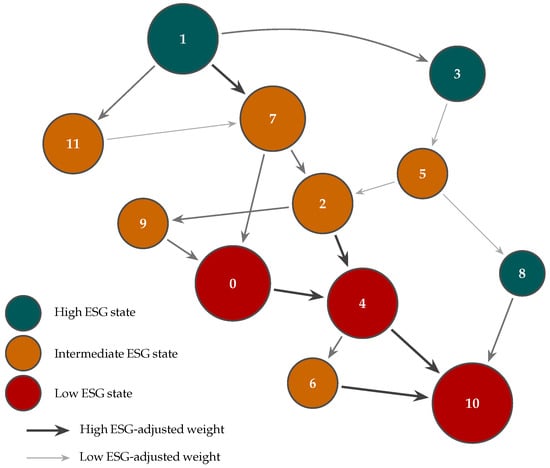
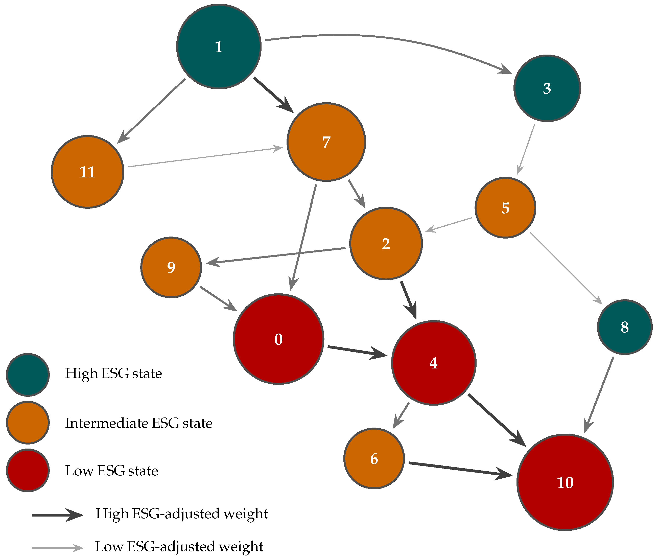
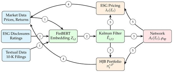
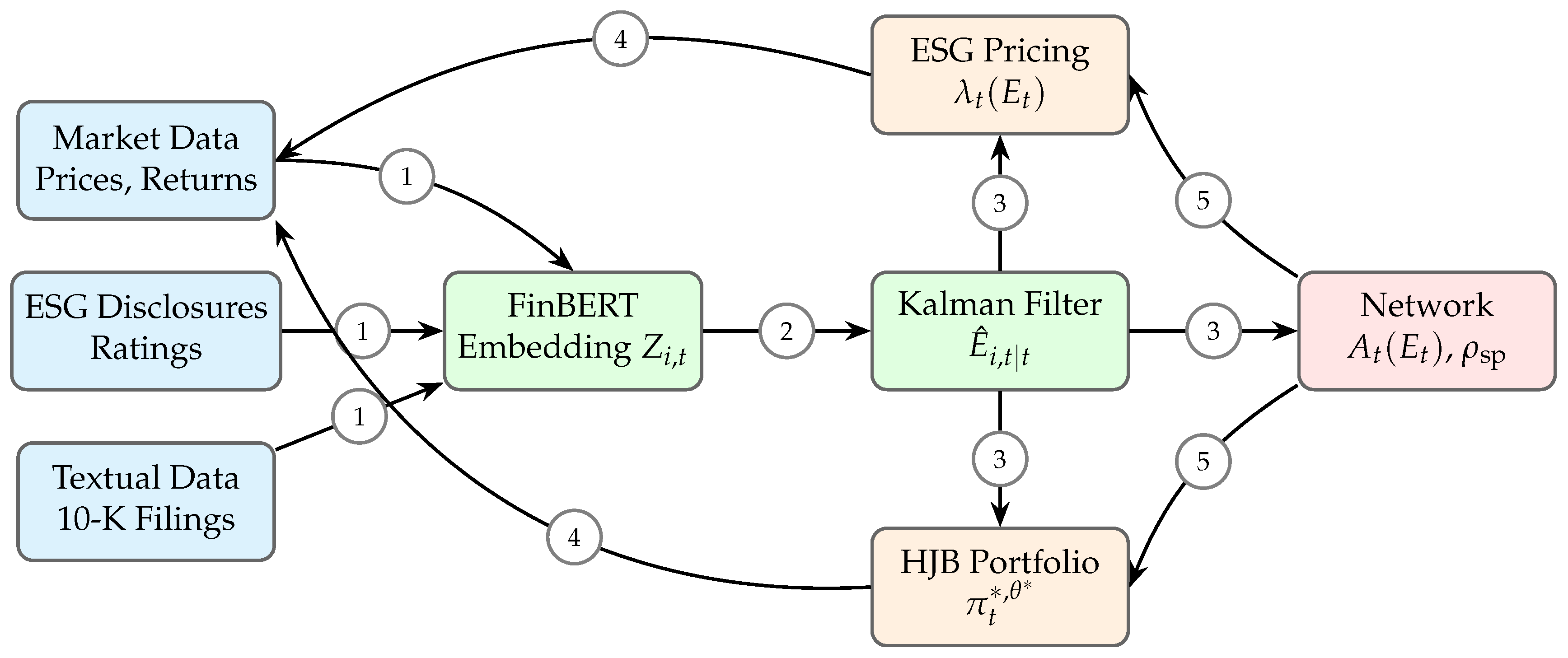

Disclaimer/Publisher’s Note: The statements, opinions and data contained in all publications are solely those of the individual author(s) and contributor(s) and not of MDPI and/or the editor(s). MDPI and/or the editor(s) disclaim responsibility for any injury to people or property resulting from any ideas, methods, instructions or products referred to in the content. |
© 2026 by the author. Licensee MDPI, Basel, Switzerland. This article is an open access article distributed under the terms and conditions of the Creative Commons Attribution (CC BY) license.