Volatility Specification and Deep Learning Anomaly Detection: Robustness of Transformer Architectures to GARCH Model Choice

Abstract

Modern financial risk management increasingly relies on transformer-based anomaly detection, although the sensitivity of these methods to the underlying volatility model specifications remains unexplored. This study thoroughly compares four GARCH variants—symmetric GARCH and asymmetric specifications (EGARCH, GJR-GARCH, APARCH)—across two state-of-the-art transformer architectures (TranAD for point anomalies, VTT for regime detection) using S&P 500 returns spanning 1980 to 2026. The investigation addresses a fundamental question for practitioners integrating econometric and deep learning methods: does the additional complexity of asymmetric volatility modeling yield meaningfully different anomaly detection when passed through transformer architectures? The analysis reveals that the GARCH specification affects anomaly severity rankings rather than detection consensus, with high cross-model agreement (minimum Jaccard of 0.88 for TranAD and 0.76 for VTT) despite statistically significant differences in score distributions. Asymmetric models exhibit extended post-crisis sensitivity, driven by their stronger response to negative shocks—the leverage effect captured by the GJR-GARCH threshold term—rather than by greater persistence; indeed, the symmetric GARCH exhibits the longest half-life. This enables specification selection based on risk philosophy: conservative monitoring via GJR-GARCH or efficient normalization via symmetric specifications. The choice of detection method—point versus regime identification—proves more consequential for anomaly detection performance than volatility model specification.

1. Introduction

Deep learning-based anomaly detection is central to contemporary financial risk management, with transformer architectures representing the current state of the art (Kang & Kang, 2024; Tuli et al., 2022). These approaches require conditional volatility estimates as input features, which are traditionally obtained from GARCH-family models (Bollerslev, 1986; Glosten et al., 1993; Nelson, 1991). Recent studies have demonstrated the successful integration of GARCH and transformer architectures for volatility prediction (Petrosino et al., 2025), yet the sensitivity of transformer-based anomaly detection to underlying GARCH specification remains unexplored. This gap is consequential: GARCH variants encode fundamentally different stylized facts—symmetric GARCH assumes equal volatility responses to positive and negative shocks, whereas asymmetric specifications (EGARCH, GJR-GARCH, APARCH) explicitly capture leverage effects, in which adverse shocks increase volatility more than positive shocks (Black, 1976; Campbell & Hentschel, 1992). When transformer architectures learn patterns from GARCH-derived features, does specification choice materially affect which market periods are flagged as anomalous?

This study systematically compares anomaly detection performance across four GARCH specifications (GARCH, EGARCH, GJR-GARCH, APARCH) using two state-of-the-art transformer methods—TranAD for point anomaly detection and VTT for regime-level detection—on S&P 500 daily returns spanning four decades (1980–2026). Three methodological considerations are addressed. First, volatility persistence parameters determine the speed of normalization following shocks, with half-lives ranging from roughly 37 to 74 trading days across specifications. This variation may affect the duration for which recovery phases are flagged as anomalous. Second, asymmetric models capture economically meaningful dynamics such as leverage effects, shock persistence, and threshold responses, which symmetric GARCH models abstract into higher unconditional volatility parameters. Third, percentile-based anomaly thresholds may exhibit differential sensitivity to nuances in volatility estimation. If the choice of GARCH specification affects score distributions more than relative rankings, detection sets may remain robust despite differences in specifications. Detection thresholds are set at the 95th percentile of validation-period scores, adapting the peak-over-threshold principle of Siffer et al. (2017) to a fixed validation quantile, which we found to be more stable for the heavy-tailed score distributions in this study, and ensuring consistent exceedance rates across specifications.

Both detection methods analyze standardized residuals and conditional volatility across all four GARCH specifications. This approach enables direct assessment of the impact of specification choice on detection consensus, temporal concentration patterns, and economic interpretation. The test period encompasses multiple market regimes, including the COVID-19 pandemic, the 2022 inflation spike, and the 2025 “Liberation Day” tariff crisis, providing diverse stress scenarios to assess cross-model stability. Such episodes are known to reshape volatility dynamics, and GARCH-family models have been used to study how volatility behaves and propagates during periods of financial stress (Nogueira & Madaleno, 2022).

This research makes three principal contributions. Methodologically, it provides the first systematic comparison of the impact of GARCH specifications on deep learning-based anomaly detection, assessing whether advanced volatility modeling influences machine learning outputs or whether simpler specifications suffice. This addresses a fundamental question for practitioners integrating econometric and machine learning methods: does the additional complexity of asymmetric GARCH models, including leverage parameters, threshold effects, and power transformations, lead to meaningfully different anomaly detection when filtered through transformer architectures? Empirically, the study determines whether detection consensus or method-specific sensitivity prevails when combining volatility modeling with deep learning, with implications for model selection and validation strategies in financial surveillance systems. In practice, the framework supports informed specification choices by quantifying the trade-offs among model complexity, economic interpretability, and detection performance, thereby providing actionable guidance for risk management applications.

The findings complement recent research on anomaly classification by investigating whether specifying input volatility influences which periods are identified for classification. Understanding this relationship is essential for developing robust financial monitoring systems that maintain reliability across varying modeling choices.

The paper proceeds as follows. Section 2 presents the volatility modeling framework, detailing the mathematical specifications and estimation procedures for the four GARCH variants. Section 3 describes the TranAD architecture for point anomaly detection. Section 4 presents the VTT framework for regime detection. Section 5 reports empirical results, comparing detection performance across specifications and providing economic interpretation of detected events. Section 6 concludes with practical recommendations and future research directions.

2. Volatility Modeling Framework

We employ four GARCH-family models to estimate conditional volatility: GARCH(1,1) (Bollerslev, 1986), EGARCH(1,1) (Nelson, 1991), GJR-GARCH(1,1) (Glosten et al., 1993), and APARCH(1,1,1) (Ding et al., 1993). These models offer distinct capabilities for capturing volatility asymmetry and enable a comprehensive comparison between symmetric and asymmetric specifications, with mixed empirical evidence across several markets (Bose & Rahman, 2022).

2.1. GARCH(1,1) Model Specification

2.1.1. Mathematical Foundation and Model Specification

Building on the autoregressive conditional heteroskedasticity (ARCH) model of Engle (1982), the GARCH(1,1) model, first introduced by Bollerslev (1986) and further developed by Francq and Zakoïan (2019), belongs to the family of observation-driven models, which assume that volatility ${\sigma }_t$ is conditionally determined by past information and driven by observed returns $r_t=log(P_t)-log(P_{t-1})$ for an asset price series $(P_t)$ as follows:

$$\begin{array}{cc}\hfill r_t& =\mu +{ϵ}_t\hfill \\ \hfill {ϵ}_t& ={\sigma }_t{z}_t,z_t\sim \mathrm{iid}(0,1)\hfill \\ \hfill {\sigma }_t^2& =\omega +\alpha {ϵ}_{t-1}^2+\beta {\sigma }_{t-1}^2\hfill \end{array}$$

(1)

where $\mu$ denotes the unconditional mean parameter, ${ϵ}_t$ represents the innovation process, and ${\sigma }_t$ is the conditional standard deviation. The variable $z_t$ refers to standardized residuals. The parameters $\omega$, $\alpha$, and $\beta$ are real parameters with constraints $\omega >0$, $\alpha \ge 0$, $\beta \ge 0$, and $\alpha +\beta <1$.

This specification ensures that ${\sigma }_t>0$ and provides stationarity, making the model robust in capturing volatility clustering and heteroskedasticity. Moreover, as an observation-driven model, the GARCH(1,1) model conditions on past observable data, making it computationally efficient and suitable for financial time series analysis (Francq & Zakoïan, 2019).

2.1.2. Quasi-Maximum Likelihood Estimation

Following Francq and Zakoïan (2019), the model employs quasi-maximum likelihood estimation, which yields consistent and asymptotically normal parameter estimates without imposing strict distributional assumptions on the innovation process $z_t$. The quasi-log-likelihood function for the observed sample $(r_1,r_2,\dots ,r_T)$ is defined as follows:

$${\mathcal{L}}_T^{\mathrm{GARCH}}(\mathit{\theta })=-{\displaystyle \frac{1}{2}}{\displaystyle \sum _{t=1}^T}{\ell }_t(\mathit{\theta })$$

(2)

where $\mathit{\theta }={(\mu ,\omega ,\alpha ,\beta )}^{\prime }$ denotes the parameter vector, T is the sample size, and ${\ell }_t(\mathit{\theta })$ indicates the individual log-likelihood contribution at time t, defined as

$${\ell }_t(\mathit{\theta })=ln(2\pi )+ln({\sigma }_t^2(\mathit{\theta }))+{\displaystyle \frac{{(r_t-\mu )}^2}{{\sigma }_t^2(\mathit{\theta })}}$$

(3)

where ${\sigma }_t^2(\mathit{\theta })$ denotes the conditional variance as a function of the parameter vector $\mathit{\theta }$, computed recursively via Equation (1). The QMLE estimator is obtained by maximizing the quasi-log-likelihood function:

$${\widehat{\mathit{\theta }}}_T=arg\underset{\mathit{\theta }\in \mathrm{\Theta }}{max}{\mathcal{L}}_T^{\mathrm{GARCH}}(\mathit{\theta })$$

(4)

where $\mathrm{\Theta }$ represents the parameter space that satisfies the stationarity and positivity constraints.

2.1.3. Robust Variance Initialization Strategy

Following Fiorentini et al. (1996) and Francq and Zakoïan (2019), the methodology implements a hierarchical variance initialization strategy to guarantee numerical stability. The initial conditional variance ${\sigma }_1^2$ is computed using a three-tier approach for the recursive computation ${\sigma }_t^2=\omega +\alpha {ϵ}_{t-1}^2+\beta {\sigma }_{t-1}^2$, starting at $t=2$:

$${\sigma }_1^2=\left\{\begin{array}{cc}{\displaystyle \frac{\omega }{1-\alpha -\beta }}\hfill & \mathrm{if}\alpha +\beta <0.999\mathrm{and}{\displaystyle \frac{\omega }{1-\alpha -\beta }}>0\hfill \\ {\displaystyle \frac{1}{T-1}}{\displaystyle {\sum }_{t=1}^T}{(r_t-\overline{r})}^2\hfill & \mathrm{if}\mathrm{first}\mathrm{condition}\mathrm{fails}\hfill \\ max\{{(r_1-\mu )}^2,{10}^{-6}\}\hfill & \mathrm{otherwise}\hfill \end{array}\right.$$

(5)

where $\overline{r}={\displaystyle \frac{1}{T}}{\sum }_{t=1}^T{r}_t$ is the sample mean, and ${10}^{-6}$ is a numerical stability constant.

2.2. EGARCH(1,1) Model Specification

2.2.1. Mathematical Foundation and Model Specification

The Exponential GARCH model introduced by Nelson (1991) allows for asymmetric volatility responses through a loglinear specification. For observed returns defined as $r_t=log(P_t)-log(P_{t-1})$, the EGARCH(1,1) model is specified as follows:

$$\begin{array}{cc}\hfill r_t& =\mu +{ϵ}_t\hfill \\ \hfill {ϵ}_t& ={\sigma }_t{z}_t,z_t\sim \mathrm{iid}(0,1)\hfill \\ \hfill log({\sigma }_t^2)& =\omega +\beta log({\sigma }_{t-1}^2)+g(z_{t-1})\hfill \end{array}$$

(6)

where the innovation function $g(z_{t-1})$ is given by

$$g(z_{t-1})=\gamma z_{t-1}+\alpha \left[|z_{t-1}|-\mathbb{E}|z_{t-1}|\right]$$

(7)

Under the normality assumption, $\mathbb{E}|z_{t-1}|=\sqrt{2/\pi }\approx 0.7979$. The parameter $\gamma$ captures asymmetry; $\gamma <0$ indicates the leverage effect, whereby negative shocks increase volatility more than positive shocks. The stationarity condition is $\left|\beta \right|<1$.

2.2.2. Quasi-Maximum Likelihood Estimation

The EGARCH quasi-log-likelihood function is

$${\mathcal{L}}_T^{\mathrm{EGARCH}}(\mathit{\theta })=-{\displaystyle \frac{1}{2}}{\displaystyle \sum _{t=1}^T}{\ell }_t(\mathit{\theta })$$

(8)

where $\mathit{\theta }={(\mu ,\omega ,\alpha ,\gamma ,\beta )}^{\prime }$ and ${\ell }_t(\mathit{\theta })$ is given by

$${\ell }_t(\mathit{\theta })=ln(2\pi )+log({\sigma }_t^2)+{\displaystyle \frac{{(r_t-\mu )}^2}{{\sigma }_t^2}}$$

(9)

where ${\sigma }_t^2=exp(log({\sigma }_t^2))$ with $log({\sigma }_t^2)$ computed via the EGARCH recursion in Equation (6). The QMLE estimator is

$${\widehat{\mathit{\theta }}}_T=arg\underset{\mathit{\theta }\in \mathrm{\Theta }}{max}{\mathcal{L}}_T^{\mathrm{EGARCH}}(\mathit{\theta })$$

(10)

2.2.3. Variance Initialization Strategy

For the EGARCH model, the initial log-variance is computed as

$$log({\sigma }_1^2)=log\left({\displaystyle \frac{1}{T-1}}{\displaystyle \sum _{t=1}^T}{(r_t-\overline{r})}^2\right)$$

(11)

The log-variance specification ensures ${\sigma }_t^2>0$ for all t without requiring explicit positivity constraints.

2.3. GJR-GARCH(1,1) Model Specification

2.3.1. Mathematical Foundation and Model Specification

The threshold GARCH model, as introduced by Glosten et al. (1993), incorporates asymmetric volatility responses by employing an indicator function that accounts for negative shocks:

$$\begin{array}{cc}\hfill r_t& =\mu +{ϵ}_t\hfill \\ \hfill {ϵ}_t& ={\sigma }_t{z}_t,z_t\sim \mathrm{iid}(0,1)\hfill \\ \hfill {\sigma }_t^2& =\omega +\alpha {ϵ}_{t-1}^2+\gamma I_{t-1}{ϵ}_{t-1}^2+\beta {\sigma }_{t-1}^2\hfill \end{array}$$

(12)

where $I_{t-1}=⊮({ϵ}_{t-1}<0)$ denotes an indicator function that equals one when a negative shock occurs and zero otherwise. The parameter $\gamma >0$ signifies that negative shocks exert a greater influence on volatility. The stationarity condition is $\alpha +\beta +\gamma /2<1$.

2.3.2. Quasi-Maximum Likelihood Estimation

The GJR-GARCH quasi-log-likelihood function is defined as follows:

$${\mathcal{L}}_T^{\mathrm{GJR}}(\mathit{\theta })=-{\displaystyle \frac{1}{2}}{\displaystyle \sum _{t=1}^T}{\ell }_t(\mathit{\theta })$$

(13)

where $\mathit{\theta }={(\mu ,\omega ,\alpha ,\gamma ,\beta )}^{\prime }$, and ${\ell }_t(\mathit{\theta })$ is given by

$${\ell }_t(\mathit{\theta })=ln(2\pi )+ln({\sigma }_t^2(\mathit{\theta }))+{\displaystyle \frac{{(r_t-\mu )}^2}{{\sigma }_t^2(\mathit{\theta })}}$$

(14)

where ${\sigma }_t^2(\mathit{\theta })$ is computed via the GJR-GARCH recursion specified in Equation (12). The QMLE estimator is given by

$${\widehat{\mathit{\theta }}}_T=arg\underset{\mathit{\theta }\in \mathrm{\Theta }}{max}{\mathcal{L}}_T^{\mathrm{GJR}}(\mathit{\theta })$$

(15)

2.3.3. Variance Initialization Strategy

The GJR-GARCH model adopts the same three-tier variance initialization strategy as the standard GARCH model, but applies the modified stationarity condition:

$${\sigma }_1^2=\left\{\begin{array}{cc}{\displaystyle \frac{\omega }{1-\alpha -\beta -\gamma /2}}\hfill & \mathrm{if}\alpha +\beta +\gamma /2<0.999\hfill \\ {\displaystyle \frac{1}{T-1}}{\displaystyle {\sum }_{t=1}^T}{(r_t-\overline{r})}^2\hfill & \mathrm{if}\mathrm{first}\mathrm{condition}\mathrm{fails}\hfill \\ max\{{(r_1-\mu )}^2,{10}^{-6}\}\hfill & \mathrm{otherwise}\hfill \end{array}\right.$$

(16)

2.4. APARCH(1,1,1) Model Specification

2.4.1. Mathematical Foundation and Model Specification

The Asymmetric Power ARCH model, as introduced by Ding et al. (1993), enables flexible power transformations and asymmetric responses:

$$\begin{array}{cc}\hfill r_t& =\mu +{ϵ}_t\hfill \\ \hfill {ϵ}_t& ={\sigma }_t{z}_t,z_t\sim \mathrm{iid}(0,1)\hfill \\ \hfill {\sigma }_t^{\delta }& =\omega +\alpha (|{ϵ}_{t-1}{|-\gamma {ϵ}_{t-1})}^{\delta }+\beta {\sigma }_{t-1}^{\delta }\hfill \end{array}$$

(17)

where $\delta >0$ denotes the power parameter, which is estimated from the data, and $-1<\gamma <1$ represents the asymmetry parameter. This specification encompasses several well-known models: setting $\delta =2$ and $\gamma =0$ recovers the standard GARCH model, while $\delta =1$ and $\gamma =0$ yields the Taylor/Schwert GARCH model.

2.4.2. Quasi-Maximum Likelihood Estimation

The quasi-log-likelihood function for the APARCH model is defined as follows:

$${\mathcal{L}}_T^{\mathrm{APARCH}}(\mathit{\theta })=-{\displaystyle \frac{1}{2}}{\displaystyle \sum _{t=1}^T}{\ell }_t(\mathit{\theta })$$

(18)

where $\mathit{\theta }={(\mu ,\omega ,\alpha ,\gamma ,\beta ,\delta )}^{\prime }$ denotes the parameter vector, and ${\ell }_t(\mathit{\theta })$ is specified as

$${\ell }_t(\mathit{\theta })=ln(2\pi )+ln({\sigma }_t^2(\mathit{\theta }))+{\displaystyle \frac{{(r_t-\mu )}^2}{{\sigma }_t^2(\mathit{\theta })}}$$

(19)

Here, ${\sigma }_t^2(\mathit{\theta })={({\sigma }_t^{\delta })}^{2/\delta }$, where ${\sigma }_t^{\delta }$ is computed using the APARCH recursion from Equation (17). The QMLE estimator is defined as

$${\widehat{\mathit{\theta }}}_T=arg\underset{\mathit{\theta }\in \mathrm{\Theta }}{max}{\mathcal{L}}_T^{\mathrm{APARCH}}(\mathit{\theta })$$

(20)

2.4.3. Variance Initialization Strategy

The initial powered conditional variance ${\sigma }_1^{\delta }$ is computed as

$${\sigma }_1^{\delta }={\left({\widehat{\sigma }}^2\right)}^{\delta /2}$$

(21)

Here, ${\widehat{\sigma }}^2={\displaystyle \frac{1}{T-1}}{\sum }_{t=1}^T{(r_t-\overline{r})}^2$ represents the sample variance, where $\overline{r}={\displaystyle \frac{1}{T}}{\sum }_{t=1}^T{r}_t$. Raising the sample variance to the power $\delta /2$ ensures that the initialization is consistent with the estimated power parameter $\delta \in (0.1,5.0)$ while maintaining ${\sigma }_1^{\delta }>0$. The numerical bounds ${\sigma }_1^{\delta }\in [{10}^{-10},{10}^{10}]$ are imposed to prevent computational underflow or overflow during optimization. The conditional variance at time t is subsequently recovered as ${\sigma }_t^2={({\sigma }_t^{\delta })}^{2/\delta }$ for use in the quasi-log-likelihood evaluation (18).

2.5. Numerical Optimization and Parameter Estimation

All model parameters are estimated numerically by maximizing their respective quasi-log-likelihood functions (Equations (2)–(18)). The following section details the optimization algorithm, constraint handling, initialization strategy, and convergence criteria, each of which is applied uniformly across all model specifications.

Across all specifications, the conditional mean is fixed at the training-sample mean, $\widehat{\mu }=\overline{r}$, and only the variance parameters are estimated numerically; this is asymptotically equivalent to jointly estimating a constant mean (Francq & Zakoïan, 2004).

2.5.1. Optimization Algorithm

We employ Sequential Least Squares Programming (SLSQP) (Kraft, 1988), a sequential quadratic programming method for nonlinear optimization with inequality constraints. Unlike bound-only quasi-Newton methods, SLSQP enforces the nonlinear stationarity inequalities (Section 2.5.2) directly during optimization rather than relying on box constraints alone, which is essential for the persistence restrictions of the GARCH-family specifications.

Before estimation, returns are rescaled to percentage units ($r_t\times 100$). In decimal units, the intercept $\omega$ (≈${10}^{-6}$) and the persistence parameters (≈$0.9$) differ by roughly six orders of magnitude, which ill-conditions the quasi-log-likelihood surface and can cause the optimizer to terminate at its starting values; rescaling equalizes the parameter magnitudes and restores the well-conditioned curvature. The intercept is converted back to the original return scale after estimation ($\omega \leftarrow \omega /{100}^2$ for the variance-level models, and $\omega \leftarrow \omega /{100}^{\delta }$ for APARCH).

At each iteration n, SLSQP obtains a search direction ${\mathbf{d}}_n$ by solving the quadratic-programming subproblem

$$\underset{\mathbf{d}}{min}\frac{1}{2}{\mathbf{d}}^{\top }{B}_n\mathbf{d}+\nabla F{({\mathit{\theta }}_n)}^{\top }\mathbf{d}\mathrm{s}.\mathrm{t}.g_j({\mathit{\theta }}_n)+\nabla g_j{({\mathit{\theta }}_n)}^{\top }\mathbf{d}\ge 0,j=1,\dots ,m,$$

(22)

and updates the parameter vector as

$${\mathit{\theta }}_{n+1}={\mathit{\theta }}_n+{\alpha }_n{\mathbf{d}}_n.$$

(23)

Here $F(\mathit{\theta })=-{\mathcal{L}}_T(\mathit{\theta })$ is the negative quasi-log-likelihood being minimized, $\left\{g_j\right\}$ are the stationarity inequality constraints (Section 2.5.2), $B_n$ is a positive-definite BFGS approximation to the Hessian of the Lagrangian $\mathcal{L}(\mathit{\theta },\lambda )=F(\mathit{\theta })-{\sum }_j{\lambda }_j{g}_j(\mathit{\theta })$, and ${\alpha }_n\in (0,1]$ is a step length obtained by line search on an $L_1$ merit function. The quadratic subproblem (22) is solved at each iteration, and $B_n$ is updated by the BFGS formula. Gradients of F and $g_j$ are computed numerically via forward finite differences, which provide sufficient accuracy for the smooth quasi-log-likelihood functions in GARCH specifications and avoid the complexity of implementing analytical derivatives.

2.5.2. Constraint Implementation

For models with explicit stationarity conditions, these constraints are imposed via the optimizer’s inequality-constraint mechanism instead of penalty methods. This approach ensures smooth optimization without discontinuities in the objective function near constraint boundaries. The specific implementations include

$$g_{\mathrm{GARCH}}(\mathit{\theta })=0.9999-\alpha -\beta >0$$

(24)

where the bound is slightly below unity ($0.9999$ rather than $1.0$) to ensure numerical stability as well as avoid boundary solutions.

EGARCH Constraints

The EGARCH model reaches stationarity when $\left|\beta \right|<1$. This condition is enforced through parameter bounds:

$$-0.9999<\beta <0.9999$$

(25)

The log-variance specification naturally ensures ${\sigma }_t^2>0$ for all t without requiring explicit positivity constraints on $\omega$, $\alpha$, or $\gamma$.

GJR-GARCH Constraints

The GJR-GARCH stationarity condition $\alpha +\beta +\gamma /2<1$ is implemented as

$$g_{\mathrm{GJR}}(\mathit{\theta })=0.9999-\alpha -\beta -{\displaystyle \frac{\gamma }{2}}>0$$

(26)

APARCH Constraints

The APARCH model imposes parameter bounds to maintain stable variance dynamics: $\delta \in [0.1,5.0]$ and $\gamma \in [-1,1]$, along with standard positivity constraints on $\omega$, $\alpha$, and $\beta$.

2.5.3. Multi-Start Optimization Strategy

To mitigate sensitivity to initial parameter values and increase the probability of locating the global maximum of the quasi-log-likelihood function, we use a multi-start optimization strategy described by Snyman and Fatti (1987). For each model, we select K candidate starting points ${\left\{{\mathit{\theta }}_0^{(k)}\right\}}_{k=1}^K$ based on sample moments and typical parameter intervals observed in financial return data. The number of starting points depends on model complexity: $K=3$ for symmetric models (GARCH) and $K=4$ for asymmetric models (EGARCH, GJR-GARCH, APARCH).

GARCH Starting Values

For the GARCH model with parameter vector $\mathit{\theta }={(\mu ,\omega ,\alpha ,\beta )}^{\prime }$, the three initialization strategies are

$$\begin{array}{cc}\hfill \mathrm{Strategy}1:& {\alpha }^{(1)}=0.05,{\beta }^{(1)}=0.90,{\omega }^{(1)}={\widehat{\sigma }}^2(1-{\alpha }^{(1)}-{\beta }^{(1)})\hfill \\ \hfill \mathrm{Strategy}2:& {\alpha }^{(2)}=0.03,{\beta }^{(2)}=0.94,{\omega }^{(2)}={\widehat{\sigma }}^2(1-{\alpha }^{(2)}-{\beta }^{(2)})\hfill \\ \hfill \mathrm{Strategy}3:& {\alpha }^{(3)}=0.10,{\beta }^{(3)}=0.85,{\omega }^{(3)}={\widehat{\sigma }}^2(1-{\alpha }^{(3)}-{\beta }^{(3)})\hfill \end{array}$$

(27)

where ${\widehat{\sigma }}^2={\displaystyle \frac{1}{T-1}}{\sum }_{t=1}^T{(r_t-\overline{r})}^2$ is the sample variance of the percentage-scaled training returns used for estimation (Section 2.5.1). The intercept seeds ${\omega }^{(k)}$ are therefore expressed in the same scaled units, while the $\alpha ,\beta ,\gamma ,\delta$ starting values are scale-invariant and ${\mu }^{(k)}=\overline{r}$ for all strategies.

EGARCH Starting Values

For the EGARCH model with parameter vector $\mathit{\theta }={(\mu ,\omega ,\alpha ,\gamma ,\beta )}^{\prime }$, EGARCH specifies the logarithm of the conditional variance, so its intercept $\omega$ lies on a log scale rather than the variance scale of the other models—hence, the starting values are built from $log({\widehat{\sigma }}^2)$, scaled by small empirical factors to span a plausible range of initial levels. As multi-start seeds, these values leave the final estimates unchanged. The four initialization strategies are

$$\begin{array}{cc}\hfill \mathrm{Strategy}1:& {\alpha }^{(1)}=0.1,{\gamma }^{(1)}=-0.1,{\beta }^{(1)}=0.95,{\omega }^{(1)}=log({\widehat{\sigma }}^2)\times 0.005\hfill \\ \hfill \mathrm{Strategy}2:& {\alpha }^{(2)}=0.2,{\gamma }^{(2)}=-0.05,{\beta }^{(2)}=0.90,{\omega }^{(2)}=log({\widehat{\sigma }}^2)\times 0.01\hfill \\ \hfill \mathrm{Strategy}3:& {\alpha }^{(3)}=0.15,{\gamma }^{(3)}=-0.3,{\beta }^{(3)}=0.88,{\omega }^{(3)}=log({\widehat{\sigma }}^2)\times 0.02\hfill \\ \hfill \mathrm{Strategy}4:& {\alpha }^{(4)}=0.3,{\gamma }^{(4)}=-0.1,{\beta }^{(4)}=0.75,{\omega }^{(4)}=log({\widehat{\sigma }}^2)\times 0.05\hfill \end{array}$$

(28)

These strategies span a range of persistence levels and leverage effect magnitudes commonly observed in equity return volatility.

GJR-GARCH Starting Values

For the GJR-GARCH model with parameter vector $\mathit{\theta }={(\mu ,\omega ,\alpha ,\gamma ,\beta )}^{\prime }$, the three initialization strategies are

$$\begin{array}{cc}\hfill \mathrm{Strategy}1:& {\alpha }^{(1)}=0.04,{\gamma }^{(1)}=0.05,{\beta }^{(1)}=0.88,{\omega }^{(1)}={\widehat{\sigma }}^2(1-{\alpha }^{(1)}-{\gamma }^{(1)}/2-{\beta }^{(1)})\hfill \\ \hfill \mathrm{Strategy}2:& {\alpha }^{(2)}=0.05,{\gamma }^{(2)}=0.08,{\beta }^{(2)}=0.90,{\omega }^{(2)}={\widehat{\sigma }}^2(1-{\alpha }^{(2)}-{\gamma }^{(2)}/2-{\beta }^{(2)})\hfill \\ \hfill \mathrm{Strategy}3:& {\alpha }^{(3)}=0.06,{\gamma }^{(3)}=0.10,{\beta }^{(3)}=0.85,{\omega }^{(3)}={\widehat{\sigma }}^2(1-{\alpha }^{(3)}-{\gamma }^{(3)}/2-{\beta }^{(3)})\hfill \end{array}$$

(29)

APARCH Starting Values

For the APARCH model with parameter vector $\mathit{\theta }={(\mu ,\omega ,\alpha ,\gamma ,\beta ,\delta )}^{\prime }$, the four initialization strategies explore different power parameter values:

$$\begin{array}{cc}\hfill \mathrm{Strategy}1:& {\alpha }^{(1)}=0.05,{\gamma }^{(1)}=0.3,{\beta }^{(1)}=0.85,{\delta }^{(1)}=1.5,{\omega }^{(1)}=0.01{\widehat{\sigma }}^{{\delta }^{(1)}}\hfill \\ \hfill \mathrm{Strategy}2:& {\alpha }^{(2)}=0.08,{\gamma }^{(2)}=0.5,{\beta }^{(2)}=0.88,{\delta }^{(2)}=1.8,{\omega }^{(2)}=0.02{\widehat{\sigma }}^{{\delta }^{(2)}}\hfill \\ \hfill \mathrm{Strategy}3:& {\alpha }^{(3)}=0.10,{\gamma }^{(3)}=0.7,{\beta }^{(3)}=0.90,{\delta }^{(3)}=2.0,{\omega }^{(3)}=0.05{\widehat{\sigma }}^{{\delta }^{(3)}}\hfill \\ \hfill \mathrm{Strategy}4:& {\alpha }^{(4)}=0.12,{\gamma }^{(4)}=0.4,{\beta }^{(4)}=0.80,{\delta }^{(4)}=1.2,{\omega }^{(4)}=0.001{\widehat{\sigma }}^{{\delta }^{(4)}}\hfill \end{array}$$

(30)

where $\widehat{\sigma }=\sqrt{{\widehat{\sigma }}^2}$ is the sample standard deviation.

Selection Criterion

For each model, the optimization procedure is executed from all K starting points, and the final parameter estimate is selected based on the highest achieved quasi-log-likelihood value:

$${\widehat{\mathit{\theta }}}_T={\mathit{\theta }}^{(k^{*})},\mathrm{where}{k}^{*}=arg\underset{k\in \{1,\dots ,K\}}{max}{\mathcal{L}}_T({\mathit{\theta }}^{(k)})$$

(31)

where ${\mathit{\theta }}^{(k)}$ denotes the converged parameter vector obtained from starting point ${\mathit{\theta }}_0^{(k)}$ and ${\mathcal{L}}_T(·)$ is the model-specific quasi-log-likelihood function defined in Equations (2)–(18).

2.5.4. Convergence Criteria

Optimization terminates when the relative change in the quasi-log-likelihood between successive iterations falls below a specified tolerance,

$${\displaystyle \frac{|{\mathcal{L}}_T({\mathit{\theta }}_n)-{\mathcal{L}}_T({\mathit{\theta }}_{n-1})|}{|{\mathcal{L}}_T({\mathit{\theta }}_{n-1})|}}<\mathrm{ftol},$$

(32)

with $\mathrm{ftol}={10}^{-10}$, at which point the Karush–Kuhn–Tucker conditions of the constrained problem are satisfied to within this tolerance.

Maximum iteration limits are set to 3000 for the symmetric GARCH model and 5000 for the asymmetric models to accommodate their more complex likelihood surfaces; in practice, convergence is typically achieved within 200–500 iterations.

2.6. Standard Errors and Inference

Standard errors are computed from a numerical approximation of the Hessian matrix of the negative quasi-log-likelihood at ${\widehat{\mathit{\theta }}}_T$, obtained by central finite differences. Since the standardized residuals are non-normal, the information-matrix equality fails, and the inverse Hessian alone understates the sampling uncertainty—we therefore report Bollerslev–Wooldridge robust standard errors (Bollerslev & Wooldridge, 1992), with asymptotic covariance

$$\widehat{\mathrm{Var}}({\widehat{\mathit{\theta }}}_T)=H^{-1}({\widehat{\mathit{\theta }}}_T)\widehat{B}({\widehat{\mathit{\theta }}}_T)H^{-1}({\widehat{\mathit{\theta }}}_T),$$

(33)

where H is the Hessian of the negative quasi-log-likelihood and $\widehat{B}={\sum }_t{\widehat{s}}_t{\widehat{s}}_t^{\top }$ collects the outer products of the per-observation scores. Under correct specification, $\widehat{B}=H$ and the covariance collapses to the inverse Hessian; under the documented non-normality, it retains asymptotic validity (Huber, 1981; White, 1982), and the standard errors are the square roots of its diagonal. The Hessian and score are evaluated in the percentage-scaled parameterization used for estimation, in which the problem is well-conditioned; the intercept standard error is transformed back to the original return scale (by a factor of ${100}^2$, or ${100}^{\delta }$ for APARCH), while the remaining parameters are scale-invariant. Inference rests on the asymptotic normality of the QMLE (Bollerslev & Wooldridge, 1992; Francq & Zakoïan, 2004).

2.7. Model Selection Criteria

We employ three complementary criteria for model selection.

• Likelihood Ratio Tests

For nested model comparisons, we use

$$\mathrm{LR}=2[{\mathcal{L}}_T({\widehat{\mathit{\theta }}}_{\mathrm{unrestricted}})-{\mathcal{L}}_T({\widehat{\mathit{\theta }}}_{\mathrm{restricted}})]\sim {\chi }^2(q)$$

(34)

where q is the difference in the number of parameters.

• Information Criteria

We compute

$$\begin{array}{cc}\hfill \mathrm{AIC}& =2k-2{\mathcal{L}}_T({\widehat{\mathit{\theta }}}_T)\hfill \end{array}$$

(35)

$$\begin{array}{cc}\hfill \mathrm{BIC}& =klog(T)-2{\mathcal{L}}_T({\widehat{\mathit{\theta }}}_T)\hfill \end{array}$$

(36)

where k is the number of parameters and T is the training-sample size.

2.8. Volatility Extraction for Anomaly Detection

Using the parameters estimated on the training sample, conditional-variance recursion is applied forward over the full sample $t=1,\dots ,T$ to generate the conditional volatility sequence ${\left\{{\widehat{\sigma }}_t\right\}}_{t=1}^T$ and the standardized residuals

$${\widehat{z}}_t={\displaystyle \frac{r_t-\widehat{\mu }}{{\widehat{\sigma }}_t}},$$

(37)

where $\widehat{\mu }=\overline{r}$ is the fixed training-sample mean. Because the parameters are estimated solely from the training data and then held fixed, the extracted volatility and residual series contain no look-ahead bias during the validation and test periods. These series provide the time-varying features for the transformer-based detectors: TranAD for point anomaly detection (Section 3) and VTT for regime-level detection (Section 4).

3. TranAD: Transformer-Based Point Anomaly Detection

3.1. Architectural Framework and Motivation

TranAD (Tuli et al., 2022) is a transformer-based architecture designed for unsupervised anomaly detection in multivariate time series through adversarial reconstruction learning. In contrast to recurrent models such as LSTM and GRU, which require sequential inference and are prone to vanishing gradients on long sequences, TranAD uses self-attention mechanisms. This approach enables parallel processing of entire temporal windows and captures both short-term and long-term dependencies using positional encoding (Hochreiter & Schmidhuber, 1997; Vaswani et al., 2017).

The architecture addresses three fundamental challenges in financial anomaly detection: (1) computational effectiveness, as transformers parallelize inference across GPU cores and reduce training time by up to 99% compared to recurrent baselines (Tuli et al., 2022); (2) extended dependencies, since self-attention weights allow the model to relate observations separated by arbitrary temporal distances within the input window; (3) amplification of slight anomalies, because adversarial training between dual decoders increases reconstruction errors for observations that deviate from learned normal patterns, thereby preventing the model from smoothing over mild outliers.

3.2. Multivariate Feature Construction and GARCH Integration

TranAD operates on multivariate time series, where each observation ${\mathbf{x}}_t\in {\mathbb{R}}^D$ has D features. For financial anomaly detection, a three-dimensional feature space is constructed to capture complementary aspects of return dynamics and volatility structure. Given the raw price series ${\left\{P_t\right\}}_{t=1}^T$ and GARCH-family conditional volatility estimates ${\left\{{\sigma }_t\right\}}_{t=1}^T$ from Section 2, the feature vector at timestamp t is defined as follows:

$${\mathbf{x}}_t=\left[\begin{array}{c}{r}_t\\ {\sigma }_t\\ z_t\end{array}\right]\in {\mathbb{R}}^3$$

(38)

where

$$r_t=log(P_t)-log(P_{t-1})$$

(39)

$$z_t={\displaystyle \frac{r_t-\mu }{{\sigma }_t}}$$

(40)

In this context, $r_t$ denotes log returns that represent directional price movements, ${\sigma }_t$ is the standard deviation from the GARCH model, and $z_t$ measures volatility-adjusted shocks (standardized residuals). This multivariate representation enables TranAD to detect anomalies that occur simultaneously across return magnitude, volatility level, and standard shock dimensions.

• GARCH-TranAD Interaction

The choice of a GARCH-family model directly influences anomaly detection through the conditional volatility component ${\sigma }_t$. Asymmetric specifications, such as EGARCH, GJR-GARCH, and APARCH, incorporate leverage effects: negative shocks produce higher subsequent volatility than positive shocks of equal magnitude. During market crashes, asymmetric models yield elevated estimates ${\sigma }_t$, which, in turn, reduce the magnitude of the standardized residuals $z_t={\displaystyle \frac{r_t-\mu }{{\sigma }_t}}$. This volatility normalization may lead TranAD to assign lower anomaly scores to crash events, since the corresponding high conditional volatility explains the large negative return.

Conversely, a symmetric GARCH(1,1) treats positive and negative shocks identically, potentially yielding lower ${\sigma }_t$ estimates during periods of asymmetric market stress. This results in larger $|z_t|$ values for crash events, thereby increasing their anomaly scores. Whether asymmetric volatility modeling enhances or impedes crash detection through TranAD constitutes a central empirical question of this study.

• Data Preprocessing

Each feature dimension is standardized to zero mean and unit variance using statistics computed on the training windows only, which are then applied unchanged to the validation and test windows:

$${\tilde{x}}_{t,d}={\displaystyle \frac{x_{t,d}-{\widehat{\mu }}_d^{\mathrm{train}}}{{\widehat{\sigma }}_d^{\mathrm{train}}}},d\in \{1,2,3\}$$

(41)

where ${\widehat{\mu }}_d^{\mathrm{train}}$ and ${\widehat{\sigma }}_d^{\mathrm{train}}$ denote the mean and standard deviation of feature d over the training windows. Computing the normalization statistics on the training set alone prevents information from the validation and test periods from leaking into the scaling. The standardized features ${\tilde{\mathbf{x}}}_t$ then undergo the sliding window transformation described below.

3.3. Dual Encoder–Decoder Architecture

TranAD employs two transformer encoders and two decoders trained through an adversarial game. Given the preprocessed feature time series ${\left\{{\tilde{\mathbf{x}}}_t\right\}}_{t=1}^T$ where ${\tilde{\mathbf{x}}}_t\in {\mathbb{R}}^3$, the model constructs sliding windows of length K:

$$W_t=\{{\tilde{\mathbf{x}}}_{t-K+1},\dots ,{\tilde{\mathbf{x}}}_t\}\in {\mathbb{R}}^{K\times 3}$$

(42)

yielding $T-K+1$ overlapping windows. The complete sequence until timestamp t is denoted $C_t=\{{\tilde{\mathbf{x}}}_1,\dots ,{\tilde{\mathbf{x}}}_t\}$, providing broader temporal context to the encoder. The corrected sequence-to-time mapping (Keogh & Lin, 2005) ensures position j in window $W_i$ corresponds to timestamp $i+j$:

$$\mathrm{TimeIndex}(i,j)=i+j,j\in \{0,1,\dots ,K-1\}$$

(43)

This correction prevents off-by-one errors when translating window-level anomaly scores back to daily timestamps—a subtle but critical implementation detail.

• Encoder Architecture

The first encoder processes the complete sequence C concatenated with a focus score matrix F (initially zero, purpose explained in Section 3.4). After positional encoding, the input undergoes multi-head self-attention:

$$I_1^{(1)}=\mathrm{LayerNorm}(I_1+\mathrm{MultiHeadAtt}(I_1,I_1,I_1))$$

(44)

$$I_1^{(2)}=\mathrm{LayerNorm}(I_1^{(1)}+\mathrm{FeedForward}(I_1^{(1)}))$$

(45)

where the multi-head self-attention mechanism (Vaswani et al., 2017) is defined as

$$\mathrm{MultiHeadAtt}(Q,K,V)=\mathrm{Concat}(H_1,\dots ,H_h)W^O$$

(46)

with each attention head computing

$$H_i=\mathrm{Attention}(Q{W}_i^Q,K{W}_i^K,V{W}_i^V)=\mathrm{softmax}\left({\displaystyle \frac{Q{W}_i^Q{(K{W}_i^K)}^T}{\sqrt{d_k}}}\right)V{W}_i^V$$

(47)

Here, $W_i^Q,W_i^K,W_i^V\in {\mathbb{R}}^{d_{model}\times d_k}$ are learnable projection matrices, $d_k=d_{model}/h$ is the dimension per attention head, and $h=8$ is the number of heads. The scaling factor $1/\sqrt{d_k}$ prevents dot products from growing excessively large, stabilizing gradient magnitudes during training.

The window encoder processes the input window W with masked self-attention to prevent information leakage from future timestamps during parallel training:

$$I_2^{(1)}=\mathrm{Mask}(\mathrm{MultiHeadAtt}(I_2,I_2,I_2))$$

(48)

$$I_2^{(2)}=\mathrm{LayerNorm}(I_2+I_2^{(1)})$$

(49)

$$I_2^{(3)}=\mathrm{LayerNorm}(I_2^{(2)}+\mathrm{MultiHeadAtt}(I_1^{(2)},I_1^{(2)},I_2^{(2)}))$$

(50)

The cross-attention operation in Equation (50) uses the complete sequence encoding $I_1^{(2)}$ as keys and values, while the masked window encoding $I_2^{(2)}$ serves as queries. This design enables the model to contextualize local patterns within broader temporal trends—a critical capability for distinguishing genuine anomalies from benign volatility fluctuations.

• Decoder Architecture

Two identical decoders produce independent reconstructions through a linear output layer:

$$O_i=\mathrm{FeedForward}(I_2^{(3)}),i\in \{1,2\}$$

(51)

A linear output is used rather than the sigmoid of the original TranAD formulation: the standardized features are zero-centered and unbounded, so a sigmoid’s $[0,1]$ range could not reconstruct standardized values (which take negative and greater-than-one magnitudes) and would discard the sign information in returns and residuals on which the asymmetric volatility models depend.

3.4. Two-Phase Adversarial Training

• Phase 1: Initial Reconstruction

In the first phase, both decoders independently reconstruct the input window W with focus score $F={\mathbf{0}}_{K\times 3}$:

$$O_1^{(1)},O_2^{(1)}={\mathrm{Decoder}}_1(\mathrm{Encoder}(W,\mathbf{0})),{\mathrm{Decoder}}_2(\mathrm{Encoder}(W,\mathbf{0}))$$

(52)

The reconstruction loss for each decoder measures deviation via the $L_2$-norm:

$${\mathcal{L}}_1^{(1)}=|O_1^{(1)}{-W|}_2^2,{\mathcal{L}}_2^{(1)}={|O_2^{(1)}-W|}_2^2$$

(53)

• Phase 2: Focus-Conditioned Reconstruction

In the second phase, the reconstruction error from Decoder 1 serves as a focus score that reweights attention in the encoder:

$$F=|O_1^{(1)}{-W|}_2^2$$

(54)

The model reruns inference with this focus score to produce a refined reconstruction from Decoder 2:

$${\widehat{O}}_2^{(2)}={\mathrm{Decoder}}_2(\mathrm{Encoder}(W,F))$$

(55)

This self-conditioning mechanism amplifies reconstruction errors for anomalous subsequences. High focus scores increase attention weights on specific input regions, forcing the encoder to prioritize potentially anomalous patterns that were poorly reconstructed in Phase 1.

• Adversarial Loss Formulation

The adversarial training objective is

$$\underset{{\mathrm{Decoder}}_1}{min}\underset{{\mathrm{Decoder}}_2}{max}{|{\widehat{O}}_2^{(2)}-W|}_2^2$$

(56)

Decoder 1 intends to minimize reconstruction error (producing focus score $F\approx \mathbf{0}$ for normal data), while Decoder 2 maximizes reconstruction error for focus-conditioned output. This adversarial game prevents the model from trivially reconstructing anomalies by forcing Decoder 1 to generate near-perfect reconstructions to “fool” Decoder 2.

To maintain training consistency, the combined loss employs an evolutionary weighting scheme:

$${\mathcal{L}}_1={\displaystyle \frac{1}{n}}|O_1^{(1)}{-W|}_2^2+\left(1-{\displaystyle \frac{1}{n}}\right){|{\widehat{O}}_2^{(2)}-W|}_2^2$$

(57)

$${\mathcal{L}}_2={\displaystyle \frac{1}{n}}|O_2^{(1)}{-W|}_2^2-\left(1-{\displaystyle \frac{1}{n}}\right){|{\widehat{O}}_2^{(2)}-W|}_2^2$$

(58)

where n is the training epoch. At the first epoch ($n=1$), the reconstruction term dominates ($1/n=1$), ensuring stable learning while reconstructions are still poor; as training progresses ($1/n\to 0$), the adversarial term gains weight, enabling the model to amplify anomaly reconstruction errors.

3.5. Anomaly Scoring and Threshold Selection

During inference, the anomaly score at timestamp t combines reconstruction errors from both phases:

$$A_t={\displaystyle \frac{1}{2}}|O_1^{(1)}-W_t{|}_2^2+{\displaystyle \frac{1}{2}}{|{\widehat{O}}_2^{(2)}-W_t|}_2^2$$

(59)

Days with scores exceeding a fixed threshold are flagged as outliers. The threshold $\tau$ is set as the 95th percentile of the anomaly scores computed on the validation set, and then applied without modification to the test set:

$${\mathrm{Outlier}}_t=⊮\{A_t>\tau \},\tau =Q_{0.95}\left({\left\{A_v\right\}}_{v\in \mathrm{val}}\right)$$

(60)

Calibrating the threshold on a held-out validation period, rather than on the test scores themselves, ensures that the cutoff is not tuned to the evaluation data and yields a consistent nominal detection rate across GARCH specifications. This adapts the peak-over-threshold principle of Siffer et al. (2017), used in Tuli et al. (2022), to a fixed, validation-based quantile, which we found to be more stable for the heavy-tailed financial score distributions in this study.

3.6. Interpretation as Point Anomaly Detector

TranAD’s daily-level anomaly scoring and short $K=30$ day sliding window make it a point anomaly detector: it assigns a score to each day and flags specific calendar dates, rather than labeling an entire window as anomalous. This temporal precision allows it to identify the exact days of acute market stress. Because each day is scored relative to its preceding 30-day window, extreme events remain influential for as long as they remain within that look-back window. During a crisis, consecutive days are therefore flagged individually while the shock persists, so the point-level detections naturally cluster into sustained episodes.

4. VTT-Based Anomaly Detection Framework

4.1. VTT Architecture

The Variable Temporal Transformer (VTT) is a deep learning architecture developed for multivariate time series anomaly detection via variable and temporal attention mechanisms (Kang & Kang, 2024). In contrast to recurrent models, VTT processes entire windows simultaneously using multi-head self-attention, enabling efficient capture of both intervariable dependencies and temporal patterns.

The VTT architecture consists of three components: (1) a dilated causal embedding layer that extracts multi-scale temporal features; (2) stacked VTT layers that apply variable and temporal attention in sequence; and (3) a reconstruction head that maps the learned representation back to the input space. Days are scored by reconstruction error, as detailed in Section 4.1.5.

4.1.1. Multi-Scale Feature Extraction via Dilated Convolutions

For an input window ${\mathbf{W}}_t\in {\mathbb{R}}^{N\times V}$ with $N=100$ timesteps and $V=5$ variables, VTT embeds each variable through parallel depthwise dilated causal convolutions (van den Oord et al., 2016) that capture patterns at multiple temporal scales. For each variable v, three depthwise 1D convolutions with increasing kernel size and dilation extract local, medium-, and long-range dependencies:

$${\mathbf{h}}_v^{(j)}={\mathrm{Conv}1\mathrm{D}}_{\mathrm{causal}}\left({\mathbf{W}}_t[:,v];k_j,d_j\right)\in {\mathbb{R}}^N,j=1,2,3,$$

(61)

with kernel sizes $(k_1,k_2,k_3)=(2,3,3)$ and dilation rates $(d_1,d_2,d_3)=(1,2,4)$. Each convolution is causal, implemented by left-padding the input by $(k_j-1)d_j$ so that the representation at time i depends only on times $\le i$. The three branch outputs are stacked and mapped to the model dimension by a shared linear projection:

$${\mathbf{e}}_v={\mathbf{W}}_{\mathrm{proj}}[{\mathbf{h}}_v^{(1)}\oplus {\mathbf{h}}_v^{(2)}\oplus {\mathbf{h}}_v^{(3)}]+{\mathbf{b}}_{\mathrm{proj}}\in {\mathbb{R}}^{N\times d_{\mathrm{model}}},$$

(62)

where $d_{\mathrm{model}}=16$. This dimension is kept deliberately modest: the variable attention below operates on tokens of dimension $N·d_{\mathrm{model}}$, so with a 100-day window, a large $d_{\mathrm{model}}$ is computationally intractable. The embeddings for all variables are stacked to form $\mathbf{E}\in {\mathbb{R}}^{N\times V\times d_{\mathrm{model}}}$.

4.1.2. Positional Encoding

To preserve temporal ordering, sinusoidal positional encodings are added:

$$\mathbf{PE}(i,2j)=sin\left({\displaystyle \frac{i}{{10000}^{2j/d_{\mathrm{model}}}}}\right)$$

(63)

$$\mathbf{PE}(i,2j+1)=cos\left({\displaystyle \frac{i}{{10000}^{2j/d_{\mathrm{model}}}}}\right)$$

(64)

where $i\in \{1,\dots ,N\}$ indexes the time position and $j\in \{0,\dots ,d_{\mathrm{model}}/2-1\}$ indexes the embedding dimension. The encoded representation becomes

$${\mathbf{X}}^{(0)}=\mathbf{E}+\mathbf{PE}$$

(65)

4.1.3. Variable and Temporal Attention

Each VTT layer applies variable attention and temporal attention in sequence, each wrapped in a residual connection and layer normalization, followed by a position-wise feed-forward network.

Variable Attention: To model intervariable relationships, the input ${\mathbf{X}}^{(\ell )}\in {\mathbb{R}}^{N\times V\times d_{\mathrm{model}}}$ is reshaped to treat the V variables as sequence elements, each represented by an $N·d_{\mathrm{model}}$ vector, and multi-head self-attention is applied across variables:

$${\mathbf{Z}}_{\mathrm{var}}=\mathrm{MultiHead}({\mathbf{X}}_{\mathrm{var}},{\mathbf{X}}_{\mathrm{var}}{\mathbf{X}}_{\mathrm{var}}),$$

(66)

$${\mathbf{X}}_{\mathrm{var}}=\mathrm{Reshape}({\mathbf{X}}^{(\ell )})\in {\mathbb{R}}^{V\times (N·d_{\mathrm{model}})}.$$

(67)

Temporal Attention: The variable-attention output is then reshaped to treat the N timesteps as sequence elements, each represented by a $V·d_{\mathrm{model}}$ vector, and multi-head self-attention is applied across time:

$${\mathbf{Z}}_{\mathrm{temp}}=\mathrm{MultiHead}({\mathbf{Z}}_{\mathrm{var}},{\mathbf{Z}}_{\mathrm{var}},{\mathbf{Z}}_{\mathrm{var}}),$$

(68)

$${\mathbf{Z}}_{\mathrm{var}}\in {\mathbb{R}}^{N\times (V·d_{\mathrm{model}})}.$$

(69)

A residual connection and layer normalization wrap the paired attention operations, and a position-wise feed-forward network produces the layer output:

$${\mathbf{X}}^{(\ell +1)}=\mathrm{LayerNorm}\left({\mathbf{X}}_{\mathrm{attn}}^{(\ell )}+\mathrm{FFN}({\mathbf{X}}_{\mathrm{attn}}^{(\ell )})\right),$$

(70)

where ${\mathbf{X}}_{\mathrm{attn}}^{(\ell )}$ denotes the input after the residual-wrapped variable and temporal attention, and $\mathrm{FFN}(\mathbf{x})={\mathbf{W}}_2\mathrm{GELU}({\mathbf{W}}_1\mathbf{x}+{\mathbf{b}}_1)+{\mathbf{b}}_2$.

4.1.4. Feature Construction and GARCH Integration

The original VTT is designed for generic multivariate sensor data—its benchmarks include industrial and physical systems such as water treatment and spacecraft telemetry (Kang & Kang, 2024). We adapt its feature space to financial time series by combining GARCH-family volatility estimates with range-based information from intraday highs and lows, the latter capturing volatility that close-to-close returns miss. For each GARCH-family model $m\in \{\mathrm{GARCH},\mathrm{EGARCH},\mathrm{GJR}\text{-}\mathrm{GARCH},\mathrm{APARCH}\}$, we construct a five-dimensional feature vector at each timestamp t:

$${\mathbf{x}}_t={\left[\begin{array}{ccccc}{r}_t& {\sigma }_{t,m}& z_{t,m}& h_t& {\ell }_t\end{array}\right]}^{\top },$$

(71)

where $r_t=log(P_t/P_{t-1})$ is the log return, ${\sigma }_{t,m}$ the conditional volatility from model m, $z_{t,m}=(r_t-\widehat{\mu })/{\sigma }_{t,m}$ the standardized residual, $h_t=(H_t-C_t)/C_t$ the normalized intraday high, and ${\ell }_t=(L_t-C_t)/C_t$ the normalized intraday low. The intraday range features $(h_t,{\ell }_t)$ capture volatility patterns beyond GARCH estimates, such as flash crashes or intraday reversals masked in close-to-close returns.

4.1.5. Reconstruction and Anomaly Scoring

After $L=2$ VTT layers, a linear reconstruction head maps the learned representation back to the input space:

$${\widehat{\mathbf{W}}}_t={\mathbf{W}}_{\mathrm{dec}}{\mathbf{X}}^{(L)}+{\mathbf{b}}_{\mathrm{dec}}.$$

(72)

A linear output is used rather than the bounded decoder of the original formulation, because the standardized features are zero-centered and unbounded, and a squashing nonlinearity could neither reconstruct their range nor preserve the sign information on which the volatility features depend.

The 100-day window and 50-day stride follow the original VTT formulation (Kang & Kang, 2024), which adopts these values in line with the Anomaly Transformer and related anomaly detection studies. Although VTT operates on this windowed input, it produces a score for each day rather than a single label per window. Every overlapping window is reconstructed, and the per-day reconstruction error—the mean squared error across the five variables at each timestamp—is accumulated and averaged over all windows covering that day:

$$s_t={\displaystyle \frac{1}{|{\mathcal{W}}_t|}}\sum _{w\in {\mathcal{W}}_t}\parallel {\mathbf{x}}_t^{(w)}-{\widehat{\mathbf{x}}}_t^{(w)}{\parallel }_2^2,$$

(73)

where ${\mathcal{W}}_t$ is the set of windows that cover day t, $|{\mathcal{W}}_t|$ is their number, and ${\mathbf{x}}_t^{(w)}$ and ${\widehat{\mathbf{x}}}_t^{(w)}$ are the true and reconstructed five-variable vectors for day t within window w. A day whose averaged score exceeds the 95th percentile of the validation-period scores is flagged. VTT therefore differs from TranAD not in flagging windows rather than days, but in the horizon over which each day is judged: its 100-day receptive field makes it sensitive to sustained volatility regimes, whereas TranAD’s 30-day window responds to sharper, more localized shocks.

5. Empirical Results and Discussion

5.1. Dataset Description

Our analysis employs daily closing prices for the S&P 500 index spanning 3 January 1980 through 31 March 2026, comprising 11,655 trading days. Data were sourced from Yahoo Finance (ticker^GSPC), retrieved via the yfinance library in Python 3.13. We compute continuously compounded returns as

$$r_t=ln(P_t)-ln(P_{t-1})$$

(74)

where $P_t$ denotes the closing price on day t. Additionally, we utilize daily high and low prices to construct normalized intraday range measures:

$$h_t={\displaystyle \frac{H_t-C_t}{C_t}},{\ell }_t={\displaystyle \frac{L_t-C_t}{C_t}}$$

(75)

where $H_t$, $L_t$, and $C_t$ represent the high, low, and closing prices on day t, respectively. These intraday measures capture volatility information beyond close-to-close returns and serve as additional features for the VTT model.

5.2. Computational Implementation

All four GARCH-family models were implemented from scratch in Python (NumPy/SciPy) rather than relying on packaged estimators, and their parameters were estimated by quasi-maximum likelihood estimation using Sequential Least Squares Programming (SLSQP) on the training period only, as detailed in Section 2. Each VTT model trains in under one minute on an NVIDIA T4 GPU, whereas each TranAD model requires approximately 7.5 min on a CPU; TranAD follows Tuli et al. (2022) with a sequence length $L=30$, and is trained for 40 epochs with the Adam optimizer (learning rate ${10}^{-3}$, batch size 64). VTT follows Kang and Kang (2024) with a window length $N=100$ and a 50-day stride, model dimension $d_{\mathrm{model}}=16$, trained for 80 epochs with the Adam optimizer (learning rate $3\times {10}^{-4}$, batch size 16, gradient-norm clipping at 1.0) with best-epoch early stopping. For both detectors, feature normalization statistics are computed only on the training windows and applied unchanged to the validation and test sets. Anomaly thresholds are set at the 95th percentile of each model’s validation-period day scores (19 September 2007 to 19 December 2016) and applied without modification to the test set, giving a consistent nominal exceedance rate across GARCH specifications.

5.3. Descriptive Statistics

Table 1 presents summary statistics for the S&P 500 returns series. The sample exhibits a mean daily return of 0.0354% (8.91% annualized) and a standard deviation of 1.13% (17.92% annualized). The returns demonstrate pronounced negative skewness (−1.05) and substantial excess kurtosis (21.23), which are characteristic of equity return distributions and are consistent with well-documented stylized facts (Cont, 2001). The Jarque–Bera test decisively rejects normality ($p<0.001$), motivating our use of GARCH-family models to capture time-varying volatility and heavy tails.

Table 1. Descriptive statistics: S&P 500 daily returns (1980–2026).

Statistic	Value
Panel A: Sample Characteristics
Start date	3 January 1980
End date	31 March 2026
Total observations	11,655
Sample period	46.2 years
Panel B: Return Distribution (Daily)
Mean (%)	0.0354
Median (%)	0.0591
Std Dev (%)	1.1288
Minimum (%)	$-22.90$
Maximum (%)	$+10.96$
Panel C: Annualized Metrics
Mean return (%)	8.91
Volatility (%)	17.92
Sharpe ratio a	0.497
Panel D: Higher Moments
Skewness	$-1.0457$
Excess kurtosis	21.23 b
Jarque–Bera	286,992 c
Panel E: Extreme Events
Largest drop	$-22.90\%$ (19 October 1987)
Largest gain	$+10.96\%$ (13 October 2008)

Returns computed as log-returns as defined in Section 2. ^a Sharpe ratio assumes zero risk-free rate. ^b Excess kurtosis = kurtosis − 3. ^c Jarque–Bera test rejects normality at the 1% level ($p<0.001$).

The sample encompasses several major market shocks, such as the 1987 Black Monday crash (the largest single-day drop of −22.90%), the 2008 Global Financial Crisis (the largest single-day gain of +10.96% during the recovery), the 2020 COVID-19 pandemic, the 2022 inflation and rate-tightening cycle, and market events extending through early 2026. This 46-year span provides a comprehensive evaluation period for anomaly detection methods across diverse market conditions.

5.4. Experimental Setup

We partitioned the 11,655-observation sample into three non-overlapping subsets following standard machine learning practice and the evaluation protocol of Tuli et al. (2022):

• Training set (60%): This comprised 6993 observations, covering 3 January 1980 to 18 September 2007, and was used to estimate GARCH model parameters and train TranAD and VTT neural network architectures.
• Validation set (20%): This comprised 2331 observations, covering 19 September 2007, to 19 December 2016. It was used for calibrating the 95th-percentile anomaly detection threshold for both methods. This period includes the 2008 Global Financial Crisis, supplying a diverse validation environment.
• Test set (20%): This comprised 2331 observations, covering 20 December 2016, to 31 March 2026. It was a held-out sample for final performance evaluation, encompassing the COVID-19 pandemic (2020), the 2022 inflation and rate-tightening cycle, and market events through early 2026. This set was never used for training the model or threshold calibration, ensuring genuine out-of-sample evaluation.

For TranAD with a 30-day sequence length, this partitioning yielded 6964 training sequences, 2331 validation sequences, and 2331 test sequences. For VTT with a 100-day window size and a 50-day stride, this yielded 138 training windows, 47 validation windows, and 47 test windows: a window was assigned to a partition by the position of its final observation and counted toward training only if it lay entirely within the training region, which is why these counts are smaller than a naive division of the sample would suggest. VTT was trained solely on these fully contained training windows, so no validation or test observation entered its fitting; only the scoring of days immediately adjacent to a partition boundary may draw on a window spanning that boundary. The use of 60/20/20 rather than the more common 80/20 split is deliberate: it provides a separate held-out test set, allowing us to calibrate thresholds on validation data and report final performance on truly unseen data. This addresses a major limitation of many anomaly detection studies that report performance on the same data used to select thresholds.

All GARCH-family models (GARCH, EGARCH, GJR-GARCH, APARCH) were estimated on the training set only (6993 observations) via quasi-maximum likelihood with SLSQP optimization. The estimated parameters were then held fixed and the conditional-variance recursion was rolled forward over the full sample to produce the conditional volatility estimates ${\left\{{\widehat{\sigma }}_t\right\}}_{t=1}^{11655}$ and standardized residuals ${\{{\widehat{z}}_t=(r_t-\widehat{\mu })/{\widehat{\sigma }}_t\}}_{t=1}^{11655}$, where $\widehat{\mu }=\overline{r}$ is the fixed training-sample mean. Because only training-period information enters the estimates, these features carry no look-ahead over the validation and test periods. The volatility estimates and standardized residuals were used to construct feature vectors for both anomaly detection methods:

• TranAD features (3D): $(r_t,{\widehat{\sigma }}_t,{\widehat{z}}_t)$ representing returns, conditional volatility, and standardized residuals.
• VTT features (5D): $(r_t,{\widehat{\sigma }}_t,{\widehat{z}}_t,h_t,{\ell }_t)$ augmenting TranAD features with normalized intraday high–low measures.

Critically, all feature normalization statistics (means and standard deviations for feature scaling) were computed exclusively from the training set and applied identically to the validation and test sets, preventing information leakage. Both TranAD and VTT were trained for 40 and 80 epochs, respectively, with early stopping based on validation loss. Detection thresholds were set as the 95th percentile of anomaly scores on the validation set, then applied without modification to the test set. All reported detection results in the following sections reflect performance on the held-out test period (December 2016—March 2026).

5.5. GARCH Model Estimation

We estimated four GARCH-family models to capture time-varying volatility dynamics: the symmetric GARCH(1,1) (Bollerslev, 1986) and three asymmetric specifications—EGARCH(1,1) (Nelson, 1991), GJR-GARCH(1,1) (Glosten et al., 1993), and APARCH(1,1,1) (Ding et al., 1993). All models were estimated using the quasi-maximum likelihood method. Table 2 reports parameter estimates and model selection criteria. All models exhibit high volatility persistence (between 0.98 and 0.99), consistent with long memory in equity volatility. The asymmetry parameters ($\gamma$) are statistically significant and economically meaningful across all three asymmetric specifications. For EGARCH, $\gamma =-0.078$ (negative, as in Nelson’s specification) captures the leverage effect. In the GJR-GARCH model, $\gamma =0.092$ indicates that negative shocks have a volatility impact that is approximately 5.1 times that of positive shocks. In APARCH, the substantial asymmetry coefficient ($\gamma =0.588$) combined with the power parameter ($\delta =1.18$, significantly less than 2), indicates a preference for absolute-value-type volatility dynamics with a strong asymmetric response.

Table 2. GARCH-family model estimation and comparison (training-period sample).

	GARCH	EGARCH	GJR-GARCH	APARCH
Panel A: Estimated Parameters
$\widehat{\omega }$	$1.17\times {10}^{-6}$ *	$-0.1704$ **	$1.64\times {10}^{-6}$ *	$7.40\times {10}^{-5}$ **
	$(5.36\times {10}^{-7})$	$(0.0566)$	$(6.64\times {10}^{-7})$	$(2.64\times {10}^{-5})$
$\widehat{\alpha }$	0.0698 **	0.1282 ***	0.0226 ***	0.0688 ***
	(0.0234)	(0.0279)	(0.0062)	(0.00156)
$\widehat{\beta }$	0.9209 ***	0.9814 ***	0.9154 ***	0.9269 ***
	(0.0245)	(0.0062)	(0.0217)	(0.0186)
$\widehat{\gamma }$	—	$-0.0776$ ***	0.0922 **	0.5877 ***
	—	(0.0196)	(0.0309)	(0.0817)
$\widehat{\delta }$	—	—	—	1.18 ***
	—	—	—	(0.1736)
Panel B: Persistence Metrics
Persistence a	0.991	0.981	0.984	— b
Half-life (days)	73.7	36.8	43.2	— b
Panel C: Model Fit Statistics
Log-likelihood	23,003	23,083	23,065	23,086
AIC	$-\mathrm{46,001}$	$-\mathrm{46,158}$	$-\mathrm{46,123}$	$-\mathrm{46,162}$
BIC	$-\mathrm{45,980}$	$-\mathrm{46,131}$	$-\mathrm{46,095}$	$-\mathrm{46,128}$
Panel D: Model Comparison
LR statistic vs. GARCH	—	—	124.03 ***	165.71 ***
Degrees of freedom	—	—	1	2
Panel E: Asymmetry Assessment
$\gamma$ significant?	No	Yes ***	Yes ***	Yes ***
Leverage effect	No	Yes	Yes	Yes

The conditional mean is fixed at the training-sample mean ($\widehat{\mu }=\overline{r}$); only the variance parameters are estimated. Bollerslev–Wooldridge robust standard errors are reported in parentheses (Bollerslev & Wooldridge, 1992); see Section 2.6. ***, **, and * indicate significance at the 1%, 5%, and 10% levels, respectively; all reported parameters remain statistically significant. Estimation via QMLE with SLSQP optimization, training period only. ^a Persistence: $\alpha +\beta$ (GARCH), $\beta$ (EGARCH), $\alpha +\beta +\gamma /2$ (GJR-GARCH); half-life $=ln(0.5)/ln(\mathrm{persistence})$. ^b APARCH persistence not directly comparable due to $\delta =1.18\ne 2$. LR tests apply only to the nested GJR-GARCH and APARCH ($p<0.01$); EGARCH is compared by AIC/BIC.

The estimated half-lives reveal economically significant differences in volatility dynamics across models. The standard GARCH model exhibits the longest half-life at 73.7 days, indicating that volatility shocks decay slowly. The GJR-GARCH and EGARCH models show faster mean reversion, with half-lives of 43.2 and 36.8 days, respectively. This reversal relative to the asymmetric models is consistent with the plain GARCH absorbing, through its ARCH and GARCH terms, persistence that the asymmetric specifications attribute to leverage. Models with longer half-lives assign elevated conditional volatility to more observations following a shock, which may reduce the number of periods flagged as anomalous once standardized by ${\widehat{z}}_t=(r_t-\widehat{\mu })/{\widehat{\sigma }}_t$. The APARCH half-life is not directly comparable due to its power transformation ($\delta =1.18\ne 2$).

Likelihood ratio tests decisively reject the symmetric GARCH model in favor of each asymmetric alternative (all LR statistics $>124$, $p<0.001$). APARCH attains the lowest AIC ($-\mathrm{46,162}$), with EGARCH essentially tied ($-\mathrm{46,158}$); under BIC, which penalizes APARCH’s additional power parameter more heavily, EGARCH is marginally preferred ($-\mathrm{46,131}$ versus APARCH’s $-\mathrm{46,128}$). The spread across the asymmetric models is small (AIC range $\approx 40$ points), indicating that they offer comparable improvements over GARCH and differ mainly in functional form.

Table 3 presents diagnostic tests verifying model adequacy. Ljung–Box tests on squared standardized residuals and ARCH-LM tests consistently fail to reject the null hypothesis of no remaining autocorrelation or ARCH effects (all $p>0.5$), indicating that each model effectively captures the observed volatility clustering. The standardized residuals exhibit near-zero means and unit variances as expected; however, all models retain pronounced negative skewness (≈$-0.5$ to $-0.6$) and substantial excess kurtosis (≈4 to 5), reflecting the extreme events in the training period—most notably the 1987 crash—and the inherent non-normality of equity returns. Relative to the raw returns, whose excess kurtosis reaches 21.23 (Table 1), the GARCH filtering absorbs the large majority of the unconditional tail heaviness over the same sample, yet the residuals remain distinctly non-normal. This non-normality is precisely what motivates quasi-maximum likelihood estimation, which remains consistent under distributional misspecification.

Table 3. GARCH model diagnostic tests.

Test	GARCH	EGARCH	GJR-GARCH	APARCH
Panel A: Standardized Residual Statistics
Mean	$-0.004$	$-0.005$	$-0.005$	$-0.005$
Std. dev.	0.9997	0.9997	1.0000	0.9998
Skewness	$-0.597$	$-0.545$	$-0.493$	$-0.524$
Excess kurtosis	5.28	4.40	3.95	4.21
Panel B: Ljung–Box Test (Squared Standardized Residuals)
$Q(10)$	6.09	2.92	1.78	2.91
p-value	0.808	0.983	0.998	0.983
$Q(20)$	11.07	6.19	5.30	6.07
p-value	0.944	0.999	1.000	0.999
Panel C: ARCH-LM Test
$\mathrm{LM}(5)$	4.24	1.36	0.30	1.43
p-value	0.515	0.928	0.998	0.920
$\mathrm{LM}(10)$	6.02	2.93	1.79	2.92
p-value	0.813	0.983	0.998	0.983

Ljung–Box Q-statistics test serial correlation in squared standardized residuals ${\widehat{z}}_t^2$. ARCH-LM tests for remaining ARCH effects. High p-values (>0.05) indicate no significant misspecification. All models adequately capture volatility dynamics.

While these four models produce highly correlated conditional volatility estimates (pairwise correlations $>0.95$), they differ systematically in how they treat extreme shocks due to their asymmetric specifications. These differences in volatility modeling propagate to the standardized residuals ${\widehat{z}}_t=(r_t-\widehat{\mu })/{\widehat{\sigma }}_t$, which serve as inputs to TranAD and VTT. The following analysis assesses whether these differences in volatility modeling influence the identification of anomalous market events.

5.6. Anomaly Detection Performance

5.6.1. TranAD Results

Table 4 presents TranAD detection results across the four GARCH specifications. Detection rates range narrowly from 3.43% (EGARCH) to 3.90% (GARCH), all below the 5% design level implied by the 95th-percentile threshold, indicating that the validation-calibrated threshold transfers stably to the test period without inflating the flagging rate.

Table 4. TranAD anomaly detection performance by GARCH model (test set: 2016–2026).

	GARCH(1,1)	EGARCH(1,1)	GJR-GARCH(1,1)	APARCH(1,1,1)
Panel A: Detection Performance
Outliers detected	91	80	87	87
Detection rate (%)	3.90	3.43	3.73	3.73
Threshold (95th percentile)	0.248	0.267	0.249	0.308
Panel B: Temporal Distribution (Consensus Days)
Episode 1: COVID-19 (2020)	9 March–2 June 2020    (50 consensus days)
Episode 2: 2025 tariff crisis	8 April–21 May 2025    (30 consensus days)
Panel C: Cross-Model Agreement
Jaccard index vs. GARCH	1.000	0.879	0.956	0.956
Spearman $\rho$ vs. GARCH	1.000	0.878	0.908	0.864
Common to all four models	80 dates (88% of GARCH’s 91)
Unique to model only	4	0	0	0
Panel D: Statistical Tests
Kruskal–Wallis H	129.73 ($p<0.001$)
Friedman ${\chi }^2$	816.86 ($p<0.001$)

Test set: 2331 overlapping 30-day windows. Thresholds calibrated at the 95th percentile of validation scores (2007–2016). The Jaccard index measures detection overlap (1.0 = perfect, 0 = none); Spearman $\rho$ measures rank correlation. The Kruskal–Wallis and Friedman tests confirm that score distributions differ significantly across models despite high detection consensus. Detections cluster into two sustained episodes: the COVID-19 crash and recovery (2020) and the 2025 tariff crisis. A 30-day window carries shock forward, so consecutive flagged days within an episode reflect a single continuous period of stress rather than independent anomalies.

Near-Perfect Detection Consensus: The four GARCH specifications exhibit remarkably high agreement in anomaly identification. Jaccard indices range from 0.879 to 1.000, with 88% of detected outliers (80 dates) common to all four models. GJR-GARCH and APARCH produce identical detection sets (Jaccard = 1.00), flagging the same 87 days. Only GARCH identifies four unique outliers that are not detected by any other specification. This near-consensus suggests that, for point anomaly detection with attention-based transformers, the GARCH asymmetry specification has minimal impact on which market periods are identified as anomalous. However, modest differences in ranking emerge (Spearman $\rho$ = 0.86–0.91).

Statistical Validation: To formally test whether score distributions differ across models, we conducted non-parametric tests on the anomaly scores. The Kruskal-Wallis test (Kruskal & Wallis, 1952) rejects the null hypothesis of identical distributions ($H=129.73$, $p<0.001$), confirming that GARCH specifications produce significantly different score distributions despite high detection overlap. The Friedman test (Friedman, 1937), which accounts for repeated measures within the same observations, similarly rejects the null of rank equality (${\chi }^2=816.86$, $p<0.001$). These results indicate that while models agree on which dates are anomalous (Jaccard $>0.87$), they disagree on severity rankings, a direct consequence of differing volatility estimates. For instance, GJR-GARCH’s longer half-life (43.2 days) maintains elevated volatility deeper into June, slightly dampening anomaly scores for later dates relative to EGARCH’s faster mean reversion (36.8 days).

Severity Hierarchy: The Post-Crash Window Dominates Top Rankings: Although detections span two episodes, the most severe anomalies are sharply concentrated in time: for every GARCH specification, the 10 highest-scored days fall within a single four-week window in April 2020 (collectively spanning 31 March to 27 April), immediately following the COVID-19 crash. Notably, these peak-severity days are not the largest-return days themselves—they include days with small returns (e.g., April 16, $+0.5\%$), but days whose preceding 30-day window is saturated with the extreme March crash observations, making them the hardest to reconstruct. The severity peak thus lags the crash by two to four weeks, a direct consequence of the 30-day look-back: reconstruction error is maximized when the window is fullest of crash data, then declines as the crash scrolls out of view through May and June. The four models consistently locate this peak window (all top-ten sets fall within late March–April 2020), though they do not rank the same days: GARCH, EGARCH, and APARCH peak in early April, and GJR-GARCH a week later.

Temporal Scope and Model Sensitivity: Across the 9.4-year test period, detections concentrate into two sustained episodes: the COVID-19 crash and recovery (March to June 2020) and a 2025 tariff crisis episode (April to May 2025). The 2020 cluster is more pronounced, with consensus detections beginning at the crash’s onset, including the $-10.0\%$ single-day drop on March 12 and the $-12.0\%$ drop on March 16, and persisting through the recovery into early June. The 2025 episode, flagged by all four specifications, opens with the $+9.0\%$ rebound of 9 April 2025. That detections compress into these two windows, leaving other test period events unflagged, underscores the exceptional nature of both periods, each combining high volatility with rapid directional swings in a pattern not replicated elsewhere in the sample. The modest threshold variation across models (range: 0.248 to 0.308) reflects differences in their validation-period score distributions, arising from the distinct volatility dynamics of each specification.

5.6.2. VTT Detection and Cross-Model Robustness

Table 5 presents VTT detection results across the four GARCH specifications. As VTT reconstructs 100-day windows and scores each day by its contribution to the window error, it responds to sustained regime structure rather than isolated spikes, yielding detection rates from 2.62% (GJR-GARCH) to 3.39% (GARCH). The four specifications share a common core of 57 days, but their overall agreement is lower than under TranAD: the minimum pairwise Jaccard index is 0.760 (between GJR-GARCH and EGARCH) and the mean is 0.807. To confirm that this level reflects the method rather than a single initialization, we repeated the analysis across random seeds; the minimum Jaccard was stable at 0.73 ± 0.01. This seed-stable consensus constitutes the most robust detection set, invariant to both the choice of volatility model and random initialization.

Table 5. VTT anomaly detection performance by GARCH model (test set: 2016–2026; primary run, seed 4).

	GARCH(1,1)	EGARCH(1,1)	GJR-GARCH(1,1)	APARCH(1,1,1)
Panel A: Detection Performance
Outliers detected	79	71	61	72
Detection rate (%)	3.39	3.05	2.62	3.09
Threshold (95th percentile)	0.959	0.896	0.920	0.902
Panel B: Cross-Model Agreement
Jaccard index vs. GARCH	1.000	0.786	0.772	0.841
Spearman $\rho$ vs. GARCH	1.000	0.789	0.578	0.818
Common to all four models	57 consensus dates
Unique to model only	7	2	0	0
Panel C: Statistical Tests
Kruskal–Wallis H	1291.40 ($p<0.001$)
Friedman ${\chi }^2$	1915.36 ($p<0.001$)

Test set: 2331 days (December 2016–March 2026). VTT scores each day by its averaged reconstruction error across the overlapping 100-day windows (50-day stride) that cover it; thresholds are calibrated at the 95th percentile of the validation-period day scores (19 September 2007 to 19 September 2016) and applied unchanged to the test set. The Jaccard index measures the overlap of flagged days (1 = identical, 0 = disjoint); Spearman $\rho$ measures rank correlation of day scores. Kruskal-Wallis and Friedman tests confirm that the score distributions differ significantly despite high consensus in detection.

The lower agreement is itself informative. VTT’s 100-day window draws on the conditional-volatility feature over a long horizon, so differences between GARCH specifications accumulate, producing greater divergence in the flagged days than under TranAD’s shorter window. EGARCH, the only log-variance specification, diverges most from the others, while the two power-type models cluster together. Robustness to volatility-model choice therefore depends on the detector’s temporal scope: the longer the reconstruction window, the more the choice of GARCH specification shapes which days are flagged.

5.6.3. Economic Interpretation of Detected Events

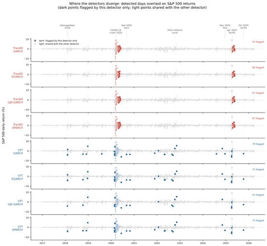
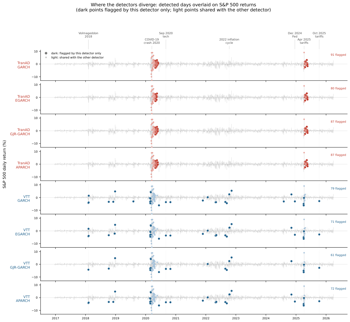
Figure 1 overlays the detections of both methods on S&P 500 returns, showing at a glance that TranAD concentrates on the two acute episodes of March 2020 and April 2025, while VTT flags a substantially wider set of days spanning the 2018 volatility shocks, the 2022 inflation cycle, and the 2024 monetary shock, with the panel counts confirming that this behavior is stable across GARCH specifications. Each date in the VTT consensus corresponds to a documented episode of market turbulence, which we review chronologically to ensure the detections are economically meaningful rather than statistical artifacts.

Figure 1. Detected anomalies overlaid on S&P 500 daily returns, by detector and GARCH specification (test period December 2016 to March 2026). Dark points are flagged by that detector alone; light points are shared with the other detector. TranAD concentrates on the 2020 and 2025 episodes, while VTT spans a broader sequence of stress events.

VTT’s long window allows it to register a broader sequence of stress than the two acute crashes, and every consensus date corresponds to a documented episode of market turbulence. The earliest, 5 February 2018 ($-4.22\%$), is the Volmageddon episode, in which the collapse of short-volatility products drove the S&P 500 to its sharpest fall since 2011. VTT further flags 10 October 2018 ($-3.38\%$), the autumn rate-driven selloff, and 26 December 2018 ($+4.80\%$), the historic rebound from the Christmas Eve low. The densest cluster is the COVID-19 crash and recovery, whose consensus spans the extreme sequence of March 2020—including 12 March ($-10.03\%$) and 16 March ($-12.80\%$), the sharpest single-day moves in the sample outside 1987—and persists into the summer, capturing the 3 September 2020 technology selloff ($-3.61\%$) and the 28 October 2020 ($-3.63\%$) pre-election drop as the recovery matured.

Beyond the crashes, VTT identifies the macroeconomic inflection points of the 2022 inflation cycle that a purely crash-focused detector would miss. It flags the early-2022 turn into monetary tightening (24 January 2022) and the hawkish Jackson Hole address of 26 August 2022 ($-3.46\%$), and then the core of the inflation cycle: 13 September 2022 ($-4.46\%$), the worst session since June 2020 after a hot inflation print; 13 October 2022 ($+2.53\%$), the intraday reversal from the bear-market low; and 10 November 2022 ($+5.36\%$), the largest rally in two years on cooler inflation data. The later consensus tracks policy-driven volatility, culminating in the 6 November 2024 ($+2.46\%$) post-election move, the April 2025 tariff shock—triggered by the U.S. administration’s announcement of broad ”reciprocal” import tariffs, which sparked a sharp global selloff and an abrupt rebound once partial exemptions were signalled—captured in full from 4 April ($-6.20\%$) through the $+9.05\%$ rebound of 9 April, and closing with 10 October 2025 ($-2.79\%$) as tensions between the United States and China over rare-earth controls resurfaced. That the four specifications agree on this economically coherent sequence, and that the agreement is seed-stable, indicates the detections are features of the data rather than artifacts of a particular volatility model.

6. Conclusions

This study investigates whether the choice of GARCH model specification materially affects anomaly detection performance when deep learning architectures rely on conditional volatility estimates as input features. Applying two state-of-the-art transformer-based methods—TranAD for point anomaly detection (Tuli et al., 2022) and VTT for detection through intervariable attention (Kang & Kang, 2024)—to S&P 500 returns with volatility estimates from four GARCH specifications, we find that the identification of major market crises is robust to specification choice. At the same time, the degree of that robustness depends on the detector’s temporal scope.

Both detectors flag the same core crisis days across all four volatility models; cross-model agreement is high, with a minimum Jaccard index of 0.879 for TranAD and 0.760 for VTT, the latter stable at $0.73\pm 0.01$ across random seeds. Statistical tests confirm that although score distributions differ significantly across specifications ($p<0.001$ for both detectors), the identity of flagged periods is largely preserved. Specification choice therefore influences the severity with which periods are scored rather than determining which periods warrant investigation, which supports the use of diverse GARCH specifications in machine learning research.

Asymmetric GARCH specifications capture economically meaningful stylized facts that have measurable consequences for post-crisis monitoring. GJR-GARCH exhibits systematic, extended sensitivity during recovery phases across both methodologies, flagging two additional dates in TranAD and one additional window in VTT (April to August 2020), with a cumulative return of $+38.37\%$ despite persistently elevated volatility. This pattern reflects the model’s asymmetric response rather than its persistence: GJR-GARCH’s half-life is moderate (43.2 trading days, against 36.8 to 73.7 across specifications), yet its stronger reaction to negative shocks ($\gamma =0.0922$) captures the well-documented leverage effect (Black, 1976; Campbell & Hentschel, 1992; Glosten et al., 1993), so heightened vigilance follows adverse returns even as volatility decays faster than under the symmetric model. Empirical evidence for news asymmetry nonetheless varies across markets (Bose & Rahman, 2022). The choice between symmetric and asymmetric specifications therefore reflects risk tolerance rather than detection accuracy: GJR-GARCH is suited to conservative tail-risk assessment with extended vigilance during recoveries, while GARCH or EGARCH facilitate efficient capital deployment with faster normalization.

The two detectors are complementary in temporal scope rather than competing in accuracy, and this distinction carries economic meaning. TranAD, over a short window, concentrates on the sharpest episodes, including the March 2020 crash and the April 2025 tariff shock, in which consecutive days of extreme moves signal a breakdown of orderly price discovery. These are events of deep Knightian uncertainty (Knight, 1921): the COVID-19 crash was a fundamental repricing in response to an exogenous shock, demanding defensive retrenchment. VTT, through its longer window, additionally captures a broader sequence of stress—the 2018 volatility shocks, the 2022 inflation cycle, and the policy-driven moves of 2024 and 2025—in which volatility is elevated, but markets remain orderly, and shocks are reversible. The 2025 tariff episode exemplifies this bounded, reversible kind of disruption: imposed under emergency economic powers and later struck down by the Supreme Court in February 2026, it was a period of policy uncertainty with recoverable parameters rather than fundamental wealth destruction. Such episodes call for tactical hedging and gradual repositioning rather than liquidation. The two detectors thus span a spectrum from acute-crash detection to sustained-regime identification, characterizing market stress at different resolutions rather than one superseding the other, and a monitoring system may profitably combine them.

Limitations and Future Research

This study focuses on S&P 500 equity returns with GARCH-family volatility models and transformer-based anomaly detection methods. Several methodological boundaries warrant acknowledgment and suggest productive directions for research.

Scope and generalization: The analysis examines a single equity index in a developed, liquid market with GARCH-family specifications. Extensions to alternative asset classes—fixed-income markets with term-structure volatility, currency pairs subject to intervention regimes, or commodities with seasonal patterns—would test whether high cross-model detection consensus generalizes beyond equity indices. Similarly, alternative volatility frameworks merit investigation: stochastic volatility models that treat volatility as latent; realized volatility from high-frequency data; and multivariate specifications (e.g., DCC, BEKK) for portfolio analysis. Whether observed robustness extends beyond conditional heteroskedasticity models remains an open empirical question.

Methodological extensions: Our focus on transformer architectures (TranAD, VTT) reflects state-of-the-art performance but excludes variational autoencoders, generative adversarial networks, and diffusion models. A systematic comparison across architectures would determine whether attention mechanisms specifically drive robustness to GARCH specification. Furthermore, while this study identifies complementary detection patterns across temporal scales—TranAD concentrating on acute episodes and VTT spanning a broader range of stress events—formal integration frameworks that weight outputs based on market microstructure conditions would enhance practical implementation. The finding that the choice of detection method dominates the choice of specification suggests that research prioritizing architectural diversity over the refinement of volatility models may yield greater marginal benefits for anomaly detection applications.

References

- Black, F. (1976). Studies of stock price volatility changes. In Proceedings of the 1976 meetings of the American Statistical Association, business and economic statistics section (pp. 177–181). American Statistical Association. [Google Scholar]
- Bollerslev, T. (1986). Generalized autoregressive conditional heteroskedasticity. Journal of Econometrics, 31(3), 307–327. [Google Scholar] [CrossRef] [Scilit]
- Bollerslev, T., & Wooldridge, J. M. (1992). Quasi-maximum likelihood estimation and inference in dynamic models with time-varying covariances. Econometric Reviews, 11(2), 143–172. [Google Scholar] [CrossRef] [Scilit]
- Bose, S., & Rahman, H. (2022). Are news effects necessarily asymmetric? Evidence from Bangladesh stock market. SAGE Open, 12(4), 21582440221127157. [Google Scholar] [CrossRef] [Scilit]
- Campbell, J. Y., & Hentschel, L. (1992). No news is good news: An asymmetric model of changing volatility in stock returns. Journal of Financial Economics, 31(3), 281–318. [Google Scholar]
- Cont, R. (2001). Empirical properties of asset returns: Stylized facts and statistical issues. Quantitative Finance, 1(2), 223–236. [Google Scholar] [CrossRef]
- Ding, Z., Granger, C. W., & Engle, R. F. (1993). A long memory property of stock market returns and a new model. Journal of Empirical Finance, 1(1), 83–106. [Google Scholar] [CrossRef] [Scilit]
- Engle, R. F. (1982). Autoregressive conditional heteroscedasticity with estimates of the variance of United Kingdom inflation. Econometrica, 50(4), 987–1007. [Google Scholar] [CrossRef] [Scilit]
- Fiorentini, G., Calzolari, G., & Panattoni, L. (1996). Analytic derivatives and the computation of GARCH estimates. Journal of Applied Econometrics, 11(4), 399–417. [Google Scholar] [CrossRef] [Scilit]
- Francq, C., & Zakoïan, J.-M. (2004). Maximum likelihood estimation of pure GARCH and ARMA-GARCH processes. Bernoulli, 10(4), 605–637. [Google Scholar] [CrossRef] [Scilit]
- Francq, C., & Zakoïan, J.-M. (2019). GARCH models: Structure, statistical inference and financial applications (2nd ed.). John Wiley & Sons. [Google Scholar] [CrossRef] [Scilit]
- Friedman, M. (1937). The use of ranks to avoid the assumption of normality implicit in the analysis of variance. Journal of the American Statistical Association, 32(200), 675–701. [Google Scholar] [CrossRef]
- Glosten, L. R., Jagannathan, R., & Runkle, D. E. (1993). On the relation between the expected value and the volatility of the nominal excess return on stocks. The Journal of Finance, 48(5), 1779–1801. [Google Scholar] [CrossRef]
- Hochreiter, S., & Schmidhuber, J. (1997). Long short-term memory. Neural Computation, 9(8), 1735–1780. [Google Scholar] [CrossRef] [Scilit] [PubMed]
- Huber, P. J. (1981). Robust statistics. Wiley Series in Probability and Statistics. John Wiley & Sons. [Google Scholar] [CrossRef] [Scilit]
- Kang, H., & Kang, P. (2024). Transformer-based multivariate time series anomaly detection using inter-variable attention mechanism. Knowledge-Based Systems, 290, 111507. [Google Scholar] [CrossRef] [Scilit]
- Keogh, E., & Lin, J. (2005). Clustering of time-series subsequences is meaningless: Implications for previous and future research. Knowledge and Information Systems, 8(2), 154–177. [Google Scholar] [CrossRef] [Scilit]
- Knight, F. H. (1921). Risk, uncertainty and profit. Houghton Mifflin. [Google Scholar]
- Kraft, D. (1988). A software package for sequential quadratic programming (Tech. Rep. No. DFVLR-FB 88-28). DLR German Aerospace Center, Institute for Flight Mechanics.
- Kruskal, W. H., & Wallis, W. A. (1952). Use of ranks in one-criterion variance analysis. Journal of the American Statistical Association, 47(260), 583–621. [Google Scholar] [CrossRef] [Scilit]
- Nelson, D. B. (1991). Conditional heteroskedasticity in asset returns: A new approach. Econometrica, 59(2), 347–370. [Google Scholar] [CrossRef] [Scilit]
- Nogueira, M. C., & Madaleno, M. (2022). Are sustainability indices infected by the volatility of stock indices? Analysis before and after the COVID-19 pandemic. Sustainability, 14(22), 15434. [Google Scholar] [CrossRef] [Scilit]
- Petrosino, L., Bacco, L., Salvati, G., Merone, M., & Papi, M. (2025). A GARCH-temporal fusion transformer model for the volatility prediction of exchange traded funds. Neural Computing and Applications, 37, 21435–21458. [Google Scholar] [CrossRef] [Scilit]
- Siffer, A., Fouque, P.-A., Termier, A., & Largouët, C. (2017). Anomaly detection in streams with extreme value theory. In Proceedings of the 23rd ACM SIGKDD international conference on knowledge discovery and data mining (pp. 1067–1075). Association for Computing Machinery. [Google Scholar] [CrossRef] [Scilit]
- Snyman, J. A., & Fatti, L. P. (1987). A multi-start global minimization algorithm with dynamic search trajectories. Journal of Optimization Theory and Applications, 54, 121–141. [Google Scholar] [CrossRef] [Scilit]
- Tuli, S., Casale, G., & Jennings, N. R. (2022). TranAD: Deep transformer networks for anomaly detection in multivariate time series data. Proceedings of the VLDB Endowment, 15(6), 1201–1214. [Google Scholar]
- van den Oord, A., Dieleman, S., Zen, H., Simonyan, K., Vinyals, O., Graves, A., Kalchbrenner, N., Senior, A., & Kavukcuoglu, K. (2016). WaveNet: A generative model for raw audio. arXiv. [Google Scholar] [CrossRef] [Scilit]
- Vaswani, A., Shazeer, N., Parmar, N., Uszkoreit, J., Jones, L., Gomez, A. N., Kaiser, Ł., & Polosukhin, I. (2017). Attention is all you need. Advances in Neural Information Processing Systems, 30, 6000–6010. [Google Scholar]
- White, H. (1982). Maximum likelihood estimation of misspecified models. Econometrica, 50(1), 1–25. [Google Scholar] [CrossRef] [Scilit]
Disclaimer/Publisher’s Note: The statements, opinions and data contained in all publications are solely those of the individual author(s) and contributor(s) and not of MDPI and/or the editor(s). MDPI and/or the editor(s) disclaim responsibility for any injury to people or property resulting from any ideas, methods, instructions or products referred to in the content. |
© 2026 by the authors. Licensee MDPI, Basel, Switzerland. This article is an open access article distributed under the terms and conditions of the Creative Commons Attribution (CC BY) license.