


Abstract
Using 2143 daily observations from January 2018 to March 2026, this study examines risk transmission among European Union Allowance (EUA) prices, green-bond indices, environmental, social, and governance (ESG) equity indices, conventional financial assets, and digital assets. The empirical design combines vector autoregression with an exogenous variable and generalised forecast-error variance decomposition (VAR-X/GFEVD) for the full-sample and rolling analyses with quantile vector autoregression with an exogenous variable and GFEVD (QVAR-X/GFEVD) for the quantile-specific analysis. The preferred eight-asset VAR-X specification produces a full-sample Total Connectedness Index (TCI) of 39.31%, while the corresponding 100-day rolling VAR-X analysis produces a mean TCI of 43.03%. The rolling TCI reaches a maximum of 54.17% on 20 July 2022 and a COVID-19-period maximum of 48.80% on 8 June 2020, indicating that system-wide connectedness increases during periods of market stress. The Cboe Volatility Index (VIX), S&P 500, and ESG equity index are consistently the dominant net transmitters, whereas EUAs, Bitcoin, crude oil, and green bonds are net receivers. The EUA net-receiver position becomes less negative after 2024, but this temporal association should not be interpreted as evidence that strengthened Phase IV provisions caused greater carbon-market stability. The quantile-specific results reveal non-monotonic state dependence, with the TCI ranging from 18.28% at τ = 0.6 to 23.52% at τ = 0.4 rather than increasing uniformly toward the lower tail.
Keywords:
carbon allowances; EU ETS; green finance; ESG; quantile VAR; connectedness; Bitcoin; geopolitical risk; climate finance; spillovers JEL Classification:
G11; G12; G14; Q54; C58; F31
1. Introduction
The interaction among climate policy, financial innovation, and cross-asset integration has created a financial environment in which environmental risk is shaped not only by regulation but also by transmission through financial markets. European Union Allowances (EUAs), which underpin the European Union Emissions Trading System (EU ETS), have consequently evolved from compliance instruments into actively traded financial assets. Their role is determined both by regulatory design and by their allocation and trading by financial intermediaries and investors. This financialisation is consistent with evidence that macrofinancial conditions and investor behaviour influence carbon prices (Chevallier, 2009; Koch et al., 2016) and that carbon risk is increasingly priced in financial markets (Bolton & Kacperczyk, 2021; Ilhan et al., 2021). Identifying the direction, magnitude, and state dependence of these spillovers is important because regulators need to assess whether external financial shocks weaken the reliability of carbon-price signals, while investors need to determine whether nominally sustainable and digital assets transmit or absorb systemic risk (Almansour et al., 2023).
A joint analysis is required because the risk role of an asset cannot be inferred solely from its bilateral correlation with another market. An asset may transmit shocks within a narrowly defined system but absorb shocks when embedded in a broader network containing equity, volatility, commodity, fixed-income, climate-finance, and digital-market variables. Moreover, average relationships may conceal materially different transmission patterns in bearish, normal, and bullish market conditions. A framework capable of identifying directional, dynamic, and quantile-dependent connectedness is therefore needed to determine which markets transmit shocks, which markets receive them, and whether these roles change across market states and regulatory periods.
The unified asset system is motivated by four complementary transmission channels. First, EUAs and WTI crude oil are linked through energy costs, emissions intensity, compliance demand, and carbon-price expectations, allowing energy-market shocks to affect the financial environment in which allowances are priced (Balcılar et al., 2016). Second, green bonds and ESG equities connect climate-related information with fixed-income and equity pricing, although their exposures differ because green bonds retain duration and credit-market characteristics whereas ESG indices remain exposed to broad equity-market repricing (Broadstock & Cheng, 2019; Reboredo, 2018). Third, the S&P 500 and VIX capture broad equity-market and risk-aversion channels, while gold and EUR/USD capture safe-haven and currency-valuation channels that may matter for a euro-denominated carbon market. Fourth, Bitcoin adds energy, environmental, global-liquidity, and continuous-trading channels through which digital-asset valuations may interact with energy prices, investor risk appetite, and sustainable-finance markets. These mechanisms do not imply causal relationships in every period; rather, they provide the economic rationale for estimating the selected assets jointly and allowing the magnitude and direction of connectedness to vary across time and market states.
Despite the growth of the connectedness literature, three limitations remain. First, carbon allowances, green bonds, ESG equities, conventional financial assets, and digital assets are commonly examined in separate or only partially overlapping systems. Second, limited evidence is available on how EUA connectedness changed following the commencement of EU ETS Phase IV in 2021 and the implementation of strengthened Phase IV provisions from 2024. Third, studies using Bitcoin frequently generalise their findings to the wider digital-asset market without establishing whether the results are robust to broader digital-market proxies.
Against this background, this study examines return-shock transmission among EUAs, green bonds, ESG equities, conventional financial assets, and digital assets from January 2018 to March 2026. It addresses three research questions. First, how are shocks transmitted among carbon, green-finance, conventional-finance, and digital-asset markets? Second, how does connectedness vary across return quantiles and over time? Third, are the principal findings robust to alternative digital-asset proxies, rolling-window lengths, lag orders, forecast horizons, and the alternative treatment of the euro/U.S. dollar (EUR/USD) exchange rate as an endogenous network node rather than as an exogenous conditioning variable?
This study makes specific contributions. First, it identifies the network position of EUAs within a jointly estimated climate-finance, conventional-finance, and digital-asset system rather than examining isolated bilateral relationships. Second, it separates pooled full-sample connectedness, local rolling dynamics, and quantile-specific state dependence, thereby distinguishing temporal variation from distributional variation. Third, it evaluates changes in EUA connectedness using statistically identified structural breaks while explicitly avoiding causal attribution to overlapping regulatory and market events. Fourth, it tests whether Bitcoin’s transmitter–receiver role remains stable under alternative digital-asset representations and alternative treatment of EUR/USD. Collectively, these features extend the contribution beyond a broader asset universe by testing the stability of network roles across time, market states, asset-system definitions, and modelling choices.
The remainder of the paper is organised as follows. Section 2 reviews the literature and develops the research gap. Section 3 describes the data and variables. Section 4 presents the methodology. Section 5 reports the empirical findings. Section 6 presents the robustness analyses. Section 7 discusses the findings, and Section 8 concludes with implications, limitations, and directions for future research.
2. Literature Review
The relevant literature can be organised into four connected themes: the financialisation and regulatory sensitivity of carbon markets; the integration of green bonds and ESG equities with conventional financial markets; the transmission channels linking digital assets with climate finance; and methodological developments in quantile and dynamic connectedness. This thematic organisation distinguishes the economic mechanisms underlying the asset relationships from the empirical methods used to measure them.
2.1. Carbon Markets, Regulatory Risk, and Financial Spillovers
From a theoretical perspective, the change can be understood in the framework of asset pricing under the influence of regulatory uncertainty and systemic risk transmission. Theoretical extensions of the intertemporal capital asset pricing model and arbitrage pricing theory indicate that climate transition risks and carbon regulatory uncertainty can be systemic risks, which impact expected returns (Bolton & Kacperczyk, 2021). The literature on financial contagion and the interconnectedness of markets also points out the role of interconnectedness in the transmission of risks across markets, especially during periods of stress, as the interconnectedness of markets enables the transmission of shocks via the dynamic network of markets (Diebold & Yilmaz, 2012, 2014).
Comparative evidence across multiple crises further shows that the intensity and direction of equity-market spillovers are strongly regime-dependent, with developed markets typically acting as dominant transmitters and geopolitically exposed markets as receivers (Shojaei et al., 2025). Taken together, this literature suggests that carbon markets, green financial instruments, and digital assets form an interconnected system in which macrofinancial and regulatory shocks may propagate asymmetrically. However, the position of individual assets within this broader transmission network remains insufficiently examined.
The empirical literature has also progressed in establishing the financial significance of carbon risk, although the literature is fragmented in terms of the asset classes and approaches used. The pioneering studies of Koch et al. (2016) reveal the critical role of regulatory actions in the formation of carbon prices in the EU ETS, whereas the study of Chevallier (2009) reveals the systematic link between EUA prices and various macroeconomic risks, including equity market volatility. Following this literature, the study of Bolton and Kacperczyk (2021) reveals the evidence of the priced risk premium of carbon emissions in the equity markets, whereas the study of Ilhan et al. (2021) reveals the evidence of the inclusion of carbon tail risk in the prices of options. With regard to firm-level effects, Nguyen and Phan (2020) report that carbon risk affects capital structure decisions. Jung et al. (2018) report an increase in the cost of debt for firms facing high levels of carbon risk. Additionally, Seltzer et al. (2021) report that climate-related regulatory pressure contributes to an increase in corporate bond spreads in environmentally stringent jurisdictions. While these papers provide further support that carbon risk is pervasive in financial markets, they do so by examining individual channels of transmission without providing an overview of all interactions between carbon permits and other financial instruments.
Recent research has begun to shed new light on the role of regulatory uncertainty as an important transmission mechanism through which carbon markets and financial valuation interact. Dewaelheyns et al. (2023) demonstrate that policy-induced carbon risk can lead to substantial valuation discounts for firms within the EU ETS, even in times of relatively low carbon prices. This supports the view that uncertainty rather than price is relevant for financial effects. This finding is further supported by Kim et al. (2015) through the cost-of-equity channel. Naegele and Zaklan (2019) demonstrate that carbon leakage adds another layer of complexity to the systemic effects of carbon pricing. The theoretical framework developed by Lian et al. (2026) advances this debate by highlighting the effects of market design and liquidity on the emergence of cooperative or fragmented pricing patterns in the carbon markets. Fragmented pricing structures may be more exposed to external financial shocks, whereas stronger regulatory design may mitigate that exposure.
Taken together, this literature demonstrates that EUA prices are influenced not only by compliance demand and abatement costs but also by regulatory uncertainty, financial-market conditions, and the design and liquidity of the carbon market. However, these studies generally examine individual pricing or financing channels rather than the position of EUAs within a broader multi-asset risk-transmission network. Earlier evidence also documents substantial return and volatility spillovers between energy and carbon markets, reinforcing the importance of analysing carbon risk within a broader financial and commodity network (Balcılar et al., 2016). Climate-related information is also reflected in asset prices and hedging demand across multiple financial markets (Engle et al., 2020; Giglio et al., 2021).
2.2. Green Bonds, ESG Equities, and Climate-Aligned Portfolios
The literature on green finance adds another layer of complexity, and results regarding the integration of sustainability-linked instruments into the financial system are inconclusive. Flammer (2021) reports that green bonds seem to be priced similarly to traditional fixed-income securities, suggesting a lack of direct link to carbon pricing mechanisms. Zerbib (2019) reports on the existence of a green bond premium, driven by investors’ preferences for sustainable investments. For instance, in equity markets, Liu et al. (2022) established that green commitments reduce stock price crash risk. Oestreich and Tsiakas (2015) proved that carbon efficiency is associated with better financial performance during EU ETS phases. Matsumura et al. (2014) established that carbon emissions disclosure has a negative effect on firm value. Brouwers et al. (2018) emphasized the role of carbon cost pass-through in financial performance. Andersson et al. (2016) proposed carbon efficiency as a hedge for climate transition risk. Despite all these contributions to climate finance literature, there is still ambiguity on whether green bonds, ESG equities, and carbon allowances constitute a cohesive market system or partially segmented markets, mainly because there is no unified analytical framework. This evidence also suggests that green bonds and ESG equities should not be treated as economically equivalent climate-finance instruments. Green bonds retain fixed-income and credit-market characteristics, whereas ESG indices remain equity instruments exposed to broad stock-market risk. Their transmitter or receiver roles may therefore differ substantially within a connectedness network. Prior evidence indicates that green bonds exhibit time-varying relationships with conventional bond and equity benchmarks and may provide distinct but state-dependent co-movement properties (Broadstock & Cheng, 2019; Reboredo, 2018). The corporate-finance literature further shows that green-bond issuance can affect shareholder value and firms’ environmental performance (Tang & Zhang, 2020).
2.3. Digital Assets and Climate-Finance Transmission Channels
The emerging literature on digital assets adds another dimension of complexity because connectedness among cryptocurrencies, decentralised finance (DeFi) instruments, and non-fungible tokens (NFTs) is heterogeneous and state-dependent. The spillovers of the volatility of Bitcoin become more pronounced during periods of financial stress, as demonstrated by Bouri et al. (2021), while the role of digital assets as transmitters or receivers of spillovers differs depending on the crisis regime, as shown by Alnafisah et al. (2025). The dynamic interdependencies within the digital asset universe are also supported by the findings of Yousaf and Yarovaya (2022) and Kumar et al. (2023), while the role of sentiment spillovers is demonstrated by Gunay et al. (2023). The interdependencies between digital assets, as demonstrated by Karim et al. (2022), Umar et al. (2022), and Corbet et al. (2022), are substantial, while Aharon and Demir (2022) and Dowling (2022) further document the relatively independent role of NFTs within the broader financial system. Moreover, the study of Naeem et al. (2021) further highlights the asymmetric efficiency of cryptocurrencies during crises. Overall, the above literature suggests that the field of digital assets is fragmented and in the process of development, with the level of integration with conventional and environmental finance markets not well understood. This state dependence is consistent with evidence that return and volatility spillovers within cryptocurrency markets intensify during periods of market stress (Koutmos, 2018).
Bitcoin may interact with carbon and green-finance markets through two principal structural channels. The first is an energy and environmental channel associated with electricity-intensive blockchain activity and the sensitivity of mining economics to energy prices and environmental regulation. The second is a global-liquidity channel through which changes in risk appetite, monetary conditions, and speculative capital flows affect both cryptocurrency and sustainable-asset valuations. These channels provide a theoretical basis for examining Bitcoin jointly with carbon allowances, green bonds, and ESG equities rather than treating its inclusion as merely exploratory.
Recent studies provide increasingly direct evidence of interactions between digital assets and environmental financial markets. Cifuentes-Faura et al. (2026) examine dynamic spillovers among carbon finance, Bitcoin, and green-energy markets. Li et al. (2023) identify quantile-dependent connectivity among equity markets, green commodities, and Bitcoin, while Hedhili Zaier et al. (2025) demonstrate that connectedness among blockchain-based assets, conventional assets, and clean and dirty energy equities strengthens under extreme market conditions. Naifar (2025) extends the literature to tokenised carbon assets, and Sahiner et al. (2026) show that financial-technology (FinTech) and equity-market shocks can propagate to blockchain-related and green-finance variables. This evidence supports the use of a multi-asset, quantile-sensitive framework but also indicates that Bitcoin-specific findings should not automatically be generalised to the entire digital-asset market.
2.4. Quantile Connectedness and Research Gap
Methodological improvements in measuring interconnectedness in finance have created a promising tool to address these issues. The connectedness approach by Diebold and Yilmaz (2012, 2014) allows for the quantification of directional spillovers between asset classes based on forecast error variance decompositions. Antonakakis et al. (2020) extend this approach to the quantile domain to allow for state-dependent interconnectedness by considering different states of the return distribution and potential asymmetries between tranquil and crisis periods. However, the evidence is not entirely uniform regarding the location, persistence, and direction of connectedness. Chatziantoniou et al. (2022) report stronger connectedness among green bonds, green equities, sustainable investments, and clean-energy markets at lower quantiles, while Khalfaoui et al. (2023) document pronounced extreme spillovers to green bonds during the COVID-19 period. Barunik et al. (2017), in turn, show that the frequency composition of spillovers changes under financial stress, with short-horizon transmission becoming particularly important. Evidence from digital-asset markets further indicates that transmitter–receiver roles can vary across crisis regimes and according to the composition of the asset system (Alnafisah et al., 2025; Hedhili Zaier et al., 2025). These findings imply that neither monotonic tail amplification nor stable transmitter–receiver classifications should be assumed a priori. The unresolved questions are therefore whether connectedness changes non-monotonically across return states, whether network roles persist through time and regulatory periods, and whether those roles remain stable when the asset universe changes. The present study advances beyond existing quantile-connectedness applications by addressing these questions jointly within a system that incorporates EU carbon allowances, green bonds, ESG equities, conventional financial assets, and alternative representations of digital assets.
Alternative dynamic approaches include dynamic conditional correlation generalized autoregressive conditional heteroskedasticity (DCC-GARCH), time-varying parameter vector autoregression (TVP-VAR) connectedness, and frequency-domain connectedness. DCC-GARCH models time-varying conditional correlations but does not directly provide the directional GFEVD measures required here (Engle, 2002). TVP-VAR connectedness allows coefficients to evolve smoothly over time but does not, by itself, identify heterogeneity across conditional return quantiles (Antonakakis et al., 2020). Frequency-domain connectedness separates short- and long-horizon transmission (Baruník & Křehlík, 2018). Because the research questions require both directional transmitter–receiver measures and heterogeneity across conditional return states within a common framework, VAR-X/GFEVD and QVAR-X/GFEVD are preferred here. The former provides interpretable directional forecast-error-variance shares for the full-sample and dynamic analyses, while the latter preserves those connectedness measures across return quantiles. Rolling-window sensitivity, structural-break identification, alternative asset universes, and frequency-domain decomposition are then used to assess whether the resulting network architecture depends on specific temporal, modelling, or frequency assumptions.
2.5. Synthesis of the Research Gap and Methodological Response
The literature establishes that carbon, green-finance, conventional-finance, and digital-asset markets are interconnected, but three issues remain insufficiently resolved. First, it is unclear whether EUAs retain the same network position across market states and over time. Second, changes observed around regulatory and crisis periods are frequently based on researcher-defined event windows rather than statistically identified shifts. Third, Bitcoin-specific conclusions may depend on the composition of the digital-asset universe and the treatment of exchange-rate movements. The empirical design addresses these gaps through full-sample VAR-X/GFEVD estimation, rolling-window analysis, quantile-specific QVAR-X/GFEVD estimation, Bai–Perron structural-break identification, alternative digital-asset systems, alternative treatment of EUR/USD, and frequency-domain decomposition. Each identified research gap is therefore linked to a corresponding empirical test. These considerations motivate both the composition of the asset system described in Section 3 and the connectedness framework developed in Section 4.
3. Data and Variables
The daily sample covers 2 January 2018 to 19 March 2026 and contains 2143 observations for each series. Major regulatory, geopolitical, monetary, and energy-market developments are used only as descriptive annotations in the rolling figures. Formal subperiod boundaries are identified statistically from the rolling connectedness series using the Bai–Perron procedure described in Section 4.4. Any temporal correspondence between an estimated break and a particular event is interpreted descriptively and does not establish causality.
The preferred specification contains eight endogenous market assets and EUR/USD as an exogenous macrofinancial conditioning variable. The EU Allowance (EUA) carbon-price series represents EU allowances traded on the European Energy Exchange and spans both Phase III and Phase IV of the EU ETS. The Bloomberg MSCI Green Bond Total Return Index tracks investment-grade debt securities issued for explicit environmental purposes by sovereigns, supranationals, and corporates. The S&P 500 Composite Index and the CBOE Volatility Index (VIX) are conventional gauges of equity market performance and aggregate investor uncertainty. The gold spot price is included as a safe-haven and inflation-hedging asset, consistent with the literature documenting gold’s properties during crisis periods (Baur & Lucey, 2010). The MSCI World ESG Leaders Index tracks the performance of companies selected according to ESG criteria, thus making it possible to directly compare ESG equity markets with dedicated carbon markets. West Texas Intermediate (WTI) crude-oil spot prices obtained from the U.S. Energy Information Administration (EIA) represent the energy-market transmission channel linking fossil fuels to carbon markets. Bitcoin is used as the baseline digital-asset proxy because it is the largest and most liquid cryptocurrency and provides a continuous daily series covering the complete sample period. However, Bitcoin alone cannot represent the heterogeneity of the wider digital-asset market. Section 6.3 therefore assesses the robustness of the findings using two alternative representations: a market-capitalisation-weighted composite of the ten largest cryptocurrencies and an expanded multi-cryptocurrency system that includes Ethereum, XRP, and Solana alongside Bitcoin. Accordingly, the baseline findings are interpreted as Bitcoin-specific unless they are reproduced across the alternative digital-asset specifications.
EUR/USD returns are included as a macrofinancial conditioning variable because EUA prices are denominated in euros, whereas several other sampled assets are quoted in US dollars. In the preferred VAR-X specification, lagged EUR/USD returns enter each equation as an exogenous conditioning variable and are excluded from the GFEVD connectedness matrix. The preferred connectedness network therefore contains eight endogenous market assets: EUAs, green bonds, the S&P 500, gold, the VIX, Bitcoin, WTI crude oil, and the ESG index. As a robustness test, Section 6.4 re-estimates the model with EUR/USD included as a ninth endogenous network node. This alternative specification evaluates whether the principal transmitter–receiver classifications depend on the treatment of exchange-rate innovations.
All price series are transformed into continuously compounded daily log returns before analysis. Table 1 reports descriptive statistics and stationarity tests for the resulting series. All series exhibit positive excess kurtosis, ranging from 1.220 for EUR/USD to 6.095 for Bitcoin, confirming the heavy-tailed nature of the return distributions. Bitcoin has the highest excess kurtosis, followed by the green bond index (5.216) and the VIX (4.555). EUA returns are modestly negatively skewed (−0.225), whereas gold displays the strongest positive skewness (0.300). The Jarque–Bera test rejects normality for every series at the 1% level. The Augmented Dickey–Fuller tests also reject the unit-root null at the 1% level under an intercept-only specification, with lag length selected using the Akaike information criterion (AIC), confirming that all log-return series are stationary. Figure 1 presents the normalized price evolution of the nine assets included in the analysis over the 2018–2026 period.
Table 1.
Descriptive Statistics and Stationarity Tests.
Figure 1.
Normalized Asset Price Evolution (2018–2026). All series rebased to 100 at 2 January 2018. Crisis shading: COVID-19 (red), Russia–Ukraine Conflict (blue), EU ETS Phase IV (green). Legend entries shown below figure. Source: Authors’ calculations based on EEX, Bloomberg, Cboe, COMEX, EIA, CoinMarketCap, ECB, and MSCI.
Table 2 reports Kendall’s rank-correlation coefficients, which are less sensitive than Pearson correlations to outliers and heavy-tailed observations. The strongest positive association is between the S&P 500 and the ESG index (), whereas the strongest negative association is between the S&P 500 and the VIX (), followed by the ESG index and the VIX (). EUA returns are positively associated with EUR/USD (), WTI crude oil (), the ESG index (), and the S&P 500 (), and negatively associated with the VIX (). The EUA–Bitcoin association is positive but comparatively weak (). The Gold–WTI crude oil correlation is the only statistically insignificant pairwise association (, ). These unconditional rank correlations describe average co-movement and do not establish directional, causal, or state-dependent connectedness.
Table 2.
Kendall Rank-Correlation Matrix of Daily Log Returns, 2018–2026.
4. Methodology
4.1. Quantile Vector Autoregression
The empirical design combines a conventional VAR-X/GFEVD model for the full-sample, rolling-window, structural-break, and robustness analyses with a QVAR-X/GFEVD extension for the quantile-specific analysis. This distinction prevents the conditional-mean VAR-X results from being conflated with the quantile-specific QVAR-X estimates. The quantile-specific analysis follows the quantile-connectedness framework of Ando et al. (2022), while the connectedness measures are constructed using the generalised forecast-error variance-decomposition approach of Diebold and Yilmaz (2012, 2014). The QVAR-X extension addresses two major limitations of the conventional ordinary-least-squares (OLS)-based VAR approach for financial returns. Firstly, OLS estimates are subject to the influence of the heavy-tailed outliers that are a feature of financial return series, as a result of the heteroscedastic and leptokurtic distributional properties of financial returns, as indicated by the results of Table 1. Secondly, OLS estimates only allow for the estimation of conditional mean relationships, which are unable to capture the asymmetric co-movement patterns that are a feature of the tails of the return distribution, which are the relevant regions for systemic risk evaluation, as indicated by the results of Table 1. Our results for the digital asset markets are consistent with the results of Alnafisah et al. (2025), while our results for the green bond markets are consistent with the results of Khalfaoui et al. (2023). The same quantile-connectedness architecture has been applied to commodity and exchange-rate systems across the COVID-19, Russia–Ukraine, and Israel–Palestine episodes, confirming its suitability for capturing regime-dependent, cross-asset transmission (Almansour et al., 2024). Intuitively, the connectedness framework measures how much of each asset’s future return uncertainty is attributable to shocks originating in the other assets in the system. The quantile extension evaluates this transmission separately under weak-return, typical-return, and strong-return states rather than assuming that the same relationships hold throughout the return distribution. An asset is classified as a net transmitter when the shocks it contributes to the rest of the system exceed the shocks it receives, whereas it is classified as a net receiver when the reverse occurs. The Total Connectedness Index summarises the average proportion of forecast-error variance attributable to cross-market shocks rather than each asset’s own innovations.
The preferred QVAR-X() specification for the vector of endogenous asset returns at quantile is expressed as:
where is an vector of endogenous asset returns; denotes lagged EUR/USD returns; is the quantile-specific coefficient vector associated with the exogenous currency variable; is the quantile-specific intercept vector; is the matrix of lag coefficients for lag ; and is the quantile-specific innovation vector. In the preferred QVAR-X specification, EUR/USD conditions the estimated relationships but is excluded from the GFEVD connectedness matrix. Each QVAR-X equation is estimated separately by linear quantile regression using the Koenker–Bassett check-loss function (Koenker & Bassett, 1978). For each conditional quantile τ, the coefficient estimates minimise the asymmetrically weighted absolute residuals associated with that quantile. The analysis uses nine equally spaced quantiles, τ ∈ {0.1, 0.2, …, 0.9}, to represent lower-tail, central, and upper-tail market states while avoiding the limited effective sample sizes associated with more extreme quantiles. Quantile-specific residuals are subsequently used to construct the innovation covariance matrix required for the GFEVD. All eight endogenous equations include one lag of the endogenous asset vector and one lag of EUR/USD returns as an exogenous conditioning variable. The QVAR-X system can be written in its quantile vector moving-average (QVMA) form as:
where Zh (τ) are the quantile-specific moving average coefficient matrices at lag h, which are recursively calculated using the QVAR coefficients. This infinite-order QVMA representation delivers the impulse responses needed for the variance decomposition.
4.2. Generalised Forecast Error Variance Decomposition
The generalized forecast error variance decomposition (GFEVD) at quantile τ and forecast horizon H, adapted from Pesaran and Shin (1998) to the quantile setting by Antonakakis et al. (2020), is:
where is an selection vector with unity in position and zeros elsewhere; is the th diagonal element of the quantile-specific innovation covariance matrix ; and is defined analogously with unity in position . A critical design feature of this decomposition is the use of generalised—rather than Cholesky-based orthogonalised—impulse responses. Because the generalised approach is order-invariant, it eliminates the requirement to impose a theory-grounded recursive causal ordering on the eight-asset endogenous connectedness system, an ordering that would be arbitrary and potentially misleading given the heterogeneous nature of the included instruments. Row-normalisation ensures that each row of the GFEVD matrix sums to unity, so that the elements may be interpreted as percentage contributions to forecast error variance.
The baseline lag order is set at p = 1 to maintain a parsimonious daily-return specification that can also be estimated reliably within the rolling windows. Because the system contains eight endogenous assets, additional lags would substantially increase the number of locally estimated coefficients and reduce the effective degrees of freedom without necessarily improving the measurement of short-horizon transmission. The forecast horizon is set at H = 10 trading days, corresponding approximately to two trading weeks and providing sufficient scope for short-run shocks to propagate through the system without placing excessive weight on distant-horizon extrapolation. These choices are not assumed to be uniquely optimal: Section 6.1 explicitly assesses p ∈ {1, 2, 3} and H ∈ {5, 10, 20}, and the resulting TCI varies by less than 0.11 percentage points across the nine specifications. The baseline choices therefore provide a parsimonious reference specification while the robustness analysis establishes that the principal conclusions do not depend materially on them.
4.3. Directional Connectedness Measures
Following Diebold and Yilmaz (2014), three scalar connectedness measures are derived from the normalised GFEVD matrix for each asset i in the system. The total directional connectedness to others, denoted TOi, aggregates the fraction of the forecast error variance of all variables j ≠ i that is attributable to shocks originating in variable i. It measures the risk that asset i propagates to the rest of the system.
The total directional connectedness from others, denoted FROMi, captures the fraction of asset i’s own forecast error variance that is explained by shocks emanating from all other assets j ≠ i. It quantifies the degree to which asset i absorbs external systemic risk.
Net total directional connectedness is defined as NETi = TOi − FROMi. When NETi > 0, asset i exports more risk to the system than it absorbs, classifying it as a net transmitter of shocks. When NETi < 0, the asset absorbs more risk than it generates and is classified as a net receiver. The system-wide Total Connectedness Index (TCI) is:
where is the number of endogenous assets in the connectedness system and is the total directional connectedness transmitted by asset to the remaining assets. The TCI is therefore the arithmetic mean of the asset-level measures. Because the directional measures are expressed as percentages, the TCI is also reported as a percentage. Values close to zero indicate near-complete market segmentation, while values approaching 100% indicate full systemic integration. All connectedness measures are computed for each return quantile τ ∈ {0.1, 0.2, …, 0.9}, enabling a comprehensive characterisation of how the risk transmission architecture varies across market states ranging from extreme bearish conditions (low τ) to extreme bullish conditions (high τ).
To capture temporal variation, the conventional VAR-X(1) model is re-estimated using a 100-trading-day rolling window that advances by one observation at each iteration. A 100-day window, corresponding to approximately five trading months, provides a compromise between local responsiveness and estimation reliability in an eight-endogenous-asset system: substantially shorter windows respond more rapidly to market movements but rely on fewer observations, whereas longer windows provide greater smoothing at the cost of obscuring shorter-lived changes in connectedness. Every window contains the same eight endogenous assets, includes lagged EUR/USD returns as an exogenous conditioning variable, and uses a 10-step forecast horizon. The 100-day choice is also consistent with established practice in the connectedness literature (Antonakakis et al., 2020; Chatziantoniou et al., 2022; Khalfaoui et al., 2023). Section 6.2 evaluates 80-, 100-, and 120-day windows and confirms that the principal transmitter–receiver classifications are not materially dependent on this choice. The full-sample quantile analysis is separate: it estimates QVAR-X models at τ ∈ {0.1, 0.2, …, 0.9} using all 2143 observations. Thus, “quantile” identifies the conditional location of the return distribution, whereas “rolling window” identifies the local time span over which the conventional VAR-X model is estimated.
4.4. Structural-Break Identification
To assess whether changes in dynamic connectedness coincide with statistically identifiable shifts rather than only researcher-defined event windows, the Bai–Perron global least-squares procedure is applied separately to the 100-day rolling TCI and rolling EUA NET series (Bai & Perron, 1998, 2003). A piecewise-linear specification allows both the intercept and deterministic time trend to change across segments. A 15% trimming parameter is imposed, corresponding to a minimum segment length of 307 rolling estimates. To retain a parsimonious structure and avoid treating short-lived fluctuations generated by overlapping rolling windows as separate regimes, the TCI specification permits a maximum of two breaks and the EUA NET specification permits one break. Break dates are obtained by globally minimising the residual sum of squares, and 95% confidence intervals are calculated using the profile-likelihood criterion. The estimated dates are used to validate and contextualise the event-based subperiod analysis; temporal correspondence with economic or regulatory events is interpreted descriptively and does not establish causality. The Bai–Perron analysis therefore serves as a formal stability diagnostic for the rolling TCI and EUA NET series. It tests for changes in the trajectories of these connectedness measures rather than coefficient-by-coefficient stability in every individual VAR-X or QVAR-X equation. Taken together, these procedures provide complementary evidence on average, state-dependent, time-varying, and structural-break-defined connectedness, which is reported in the following section.
5. Empirical Results
5.1. Full-Sample VAR-X Connectedness
Table 3 reports full-sample connectedness estimates from the preferred eight-asset VAR-X(1) specification, using a 10-step forecast horizon and lagged EUR/USD returns as an exogenous conditioning variable. The estimated TCI is 39.31%, indicating that approximately two-fifths of the forecast-error variance in the eight endogenous assets is attributable to cross-market shocks. The VIX, S&P 500, and ESG index are the principal net transmitters, whereas EUAs, green bonds, gold, Bitcoin, and WTI crude oil are net receivers. These classifications describe the relative directional position of each asset within the specified network and should not be interpreted as structural causal effects.
Table 3.
Full-Sample VAR-X Connectedness Measures (, H = 10, 2018–2026).
The VIX records the strongest net-transmitter position (NET = +18.47%), followed by the S&P 500 (+14.85%) and the ESG index (+10.77%). The dominance of the VIX is consistent with its role as a broad indicator of market uncertainty, while the transmitter positions of the S&P 500 and ESG index reflect the substantial integration of ESG equities with conventional equity-market dynamics. The ESG result qualifies the assumption that ESG screening necessarily insulates a portfolio from general financial-market shocks. It concerns directional spillover exposure and does not provide direct evidence concerning portfolio volatility, optimal asset weights, or hedge effectiveness.
Among the net receivers, WTI crude oil records the strongest negative position (NET = −10.72%), followed by Bitcoin (−10.58%), green bonds (−9.39%), EUAs (−7.58%), and gold (−5.82%). The EUA receiver position indicates that carbon-price returns absorb more forecast-error variance from the wider financial network than they transmit to it. Bitcoin’s receiver classification similarly reflects its position relative to the larger equity, volatility, commodity, and climate-finance markets included in the system; it should not be interpreted as an invariant characteristic of Bitcoin across all possible asset universes.
5.2. Dynamic Total Connectedness
Figure 2 reports the 100-day rolling TCI estimated from the preferred eight-asset VAR-X(1) specification, with lagged EUR/USD returns included as an exogenous conditioning variable and a 10-step forecast horizon. The mean rolling TCI is 43.03%, compared with the full-sample VAR-X TCI of 39.31%. These statistics measure related but different quantities. The full-sample TCI is obtained from one constant-parameter model estimated using all observations, whereas the rolling mean is the average of locally estimated 100-day models whose coefficients and innovation covariance matrices can change over time. The 3.72-percentage-point difference should therefore not be interpreted as an inconsistency between the models; rather, it indicates that average connectedness within local market environments is higher than the connectedness estimated after pooling the complete sample. The rolling TCI ranges from 30.25% to 54.17%. During the COVID-19 period, it reaches 48.80% on 8 June 2020, while its full-sample maximum of 54.17% occurs on 20 July 2022 during overlapping energy-market disruption and global monetary tightening. It subsequently reaches a minimum of 30.25% on 20 May 2025 before recovering toward the end of the sample. The shaded event periods are descriptive temporal annotations and do not identify the causal effects of individual events.
Figure 2.
Dynamic Total Connectedness Index—100-Day Rolling Window (2018–2026). The y-axis shows the percentage of each variable’s forecast-error variance explained by cross-market shocks. Shaded bands denote COVID-19 (red), Carbon Market Reform (green), the Russia–Ukraine Conflict (purple), and EU ETS Phase IV (orange). Source: Authors’ calculations.
5.3. Structural-Break and Subperiod Heterogeneity
Table 4 reports structural breaks in the rolling connectedness series. Rolling TCI breaks are identified on 7 July 2021 and 15 September 2022, while rolling EUA NET connectedness records a break on 3 June 2024. These dates coincide with the early Phase IV period, the Russia–Ukraine energy shock and monetary tightening, and strengthened Phase IV implementation, respectively. These temporal correspondences are descriptive and do not establish causal effects.
Table 4.
Bai–Perron Structural-Break Results.
Using these break dates, the sample is divided into four mutually exclusive subperiods. System-wide connectedness is highest during the second subperiod, from 7 July 2021 to 14 September 2022, when the TCI reaches 42.62%. EUAs, Bitcoin, and WTI crude oil remain net receivers throughout all four subperiods, although the magnitudes of their NET connectedness vary over time. Table 5 presents the connectedness measures across the structural-break-defined subperiods.
Table 5.
Connectedness across Structural-Break-Defined Subperiods.
Figure 3 visualises asset-level NET connectedness across the four structural-break-defined subperiods using the preferred eight-endogenous-asset VAR-X(1) specification. The S&P 500, VIX, and ESG index remain net transmitters throughout all four subperiods, whereas EUAs, green bonds, gold, Bitcoin, and WTI crude oil remain net receivers. EUR/USD is excluded because lagged EUR/USD returns enter the model as an exogenous conditioning variable. Although the magnitude of NET connectedness varies across the subperiods, the principal transmitter–receiver classifications remain stable.
Figure 3.
Net Directional Connectedness across Structural-Break-Defined Subperiods. Green cells indicate positive NET values and net-transmitter positions, red cells indicate negative NET values and net-receiver positions, and yellow cells indicate values closer to zero. The estimates are obtained from the preferred eight-endogenous-asset VAR-X(1) specification, with lagged EUR/USD returns included as an exogenous conditioning variable and a 10-step forecast horizon. Source: Authors’ calculations.
5.4. Quantile Connectedness Analysis
Table 6 and Figure 4 show that connectedness varies non-monotonically across conditional return quantiles, ranging from 18.28% at τ = 0.6 to 23.52% at τ = 0.4. The lower-tail TCI at τ = 0.1 is 23.03%, compared with 21.01% at the median quantile, τ = 0.5, and 20.55% at τ = 0.9. The lower-tail estimate is therefore moderately higher than the median and most upper-quantile estimates, but the maximum occurs at τ = 0.4. The results indicate state-dependent heterogeneity rather than a uniformly monotonic increase in connectedness toward the lower tail.
Table 6.
Quantile-Specific Total Connectedness Index.
Figure 4.
Total Connectedness Index across Return Quantiles (τ = 0.1–0.9). The figure reports the full-sample QVAR-X TCI estimated separately at each conditional return quantile. Differences across quantiles represent state-dependent connectedness and should not be interpreted as separate crisis-period subsamples. Source: Authors’ calculations.
5.5. Asset-Level Dynamics
Figure 5 reports the evolution of rolling NET connectedness for the eight endogenous assets. The transmitter–receiver positions vary over time, although the VIX, S&P 500, and ESG index generally occupy transmitter positions, while EUAs, green bonds, gold, Bitcoin, and WTI crude oil generally occupy receiver positions. EUA NET connectedness is predominantly negative, indicating that carbon-price returns generally absorb more shocks from the wider financial system than they transmit. Changes observed after 2024 coincide with strengthened Phase IV implementation but should not be interpreted as evidence of a causal regulatory effect.
Figure 5.
Dynamic Net Directional Connectedness by Asset 100—Day Rolling Window (2018–2026). Shaded bands denote COVID–19 (red), Carbon Market Reform (green), the Russia–Ukraine Conflict (purple), and EU ETS Phase IV (orange). Source: Authors’ calculations.
Bitcoin is a net receiver in the preferred broad asset system and across the four structural-break-defined subperiods, but it becomes a net transmitter when the system is expanded to include several smaller cryptocurrency assets. This difference indicates that Bitcoin’s transmitter–receiver classification depends on the composition of the connectedness network: it may absorb shocks from larger equity, volatility, commodity, and climate-finance markets while transmitting shocks within a more narrowly defined digital-asset bloc. These findings describe directional connectedness and do not establish Bitcoin’s diversification benefits, hedge effectiveness, or optimal portfolio role.
Figure 6 presents the full-sample VAR-X connectedness network corresponding to Table 3. The VIX, S&P 500, and ESG index are net transmitters, whereas EUAs, green bonds, gold, Bitcoin, and WTI crude oil are net receivers. EUR/USD is excluded because lagged EUR/USD returns enter the preferred VAR-X specification as an exogenous conditioning variable.
Figure 6.
Static Connectedness Network—Full Sample (2018–2026). Nodes coloured blue represent net transmitters, whereas nodes coloured red represent net receivers. Node size is proportional to the absolute value of NET, edge thickness reflects pairwise GFEVD strength, and the values inside the nodes report NET (%). Source: Authors’ calculations.
6. Robustness Tests
To assess whether the principal findings depend on particular modelling choices, five robustness exercises are conducted. These examine sensitivity to the lag order and forecast horizon, the rolling-window length, the representation of the digital-asset class, the treatment of EUR/USD, and the frequency horizon over which connectedness is measured.
6.1. Lag-Order and Forecast-Horizon Sensitivity
Table 7 examines the sensitivity of the preferred full-sample VAR-X results to alternative lag orders and forecast horizons. For VAR-X(1), the TCI is 39.30959% at , , and . For VAR-X(2), it ranges only from 39.20115% to 39.20116%, while for VAR-X(3), it ranges from 39.25235% to 39.25352%. The limited variation across forecast horizons indicates that the cumulative GFEVD has largely converged by . Across all nine specifications, the TCI varies by less than 0.11 percentage points, and the VIX, S&P 500, and ESG index remain net transmitters, while EUAs, green bonds, gold, Bitcoin, and WTI crude oil remain net receivers.
Table 7.
Robustness—Sensitivity to Lag Order and Forecast Horizon.
6.2. Rolling-Window Sensitivity
The dynamic connectedness analysis is re-estimated using rolling windows of 80, 100, and 120 trading days under the preferred eight-asset VAR-X specification. Table 8 shows that the mean rolling TCI decreases from 44.17% under the 80-day window to 43.03% under the 100-day window and 42.34% under the 120-day window, reflecting the greater smoothing associated with longer estimation windows. The maximum TCI is 56.42% for the 80-day window, 54.17% for the 100-day window, and 52.72% for the 120-day window. The dates of these maxima are 2 June 2021, 20 July 2022, and 11 August 2022, respectively. EUAs remain net receivers under all three window lengths, with mean NET connectedness ranging from −8.64% to −7.88%. Classification stability relative to the full-sample transmitter–receiver positions increases from 92.86% under the 80-day window to 97.17% under the 120-day window. The principal directional classifications are therefore robust to alternative rolling-window lengths.
Table 8.
Robustness to Alternative Rolling-Window Lengths under the Preferred VAR-X Specification.
6.3. Alternative Digital-Asset Specifications
A natural concern is that Bitcoin, although the largest and most liquid digital asset, may not adequately represent the broader digital-asset market. We therefore estimate two alternative specifications. First, Bitcoin is replaced with a market-capitalisation-weighted composite of the ten largest cryptocurrencies, while the remaining seven endogenous assets are retained. Second, Ethereum, XRP, and Solana are added alongside Bitcoin, producing an eleven-endogenous-asset system. In both specifications, lagged EUR/USD returns remain an exogenous conditioning variable and are excluded from the GFEVD connectedness matrix.
Table 9 reports the composite-substitution results. Replacing Bitcoin with the market-capitalisation-weighted digital-asset composite produces a TCI of 39.30% and composite NET connectedness of −11.00%. The composite therefore remains a net receiver, preserving the baseline digital-asset classification. However, this result is specific to the broad composite representation because Bitcoin becomes a net transmitter when smaller cryptocurrency assets are added to the system, as reported in Table 10.
Table 9.
Robustness—Digital-asset composite substitution under the preferred VAR-X specification (, ). TCI = 39.30%.
Table 10.
Robustness—Expanded multi-cryptocurrency system under the preferred VAR-X specification (, ). TCI = 49.44%.
Table 10 reports the expanded multi-cryptocurrency system. Bitcoin becomes a net transmitter (NET = +14.78%), whereas Ethereum (−1.48%), XRP (−6.35%), and Solana (−2.69%) remain net receivers. This sign reversal confirms that Bitcoin’s network position depends on the composition of the asset universe. In the preferred eight-endogenous-asset baseline system, Bitcoin absorbs shocks from larger equity, volatility, commodity, and climate-finance markets; in the expanded eleven-endogenous-asset system, it becomes the dominant transmitter within the digital-asset bloc. The TCI increases to 49.44%, while the principal non-digital transmitter–receiver classifications remain unchanged.
Table 11 reports lag-order and forecast-horizon sensitivity under the two alternative digital-asset specifications. The composite-system TCI ranges from 39.30027% to 39.46503%, while the expanded multi-cryptocurrency-system TCI ranges from 49.44430% to 49.73068%. Forecast-horizon differences remain extremely small for a given lag order, indicating rapid convergence of the cumulative GFEVD. The transmitter–receiver classifications remain unchanged across all specifications.
Table 11.
Robustness—TCI (%) sensitivity to lag order and forecast horizon across asset-universe specifications.
6.4. Alternative Endogenous Treatment of EUR/USD
The preferred specification treats lagged EUR/USD returns as an exogenous conditioning variable and excludes the exchange rate from the GFEVD connectedness matrix. To assess whether the results depend on this modelling choice, the system is re-estimated with EUR/USD included as a ninth endogenous network node. Under the alternative endogenous specification, the TCI is 37.45%. The VIX, S&P 500, and ESG index remain net transmitters, whereas EUAs, green bonds, gold, Bitcoin, WTI crude oil, and EUR/USD are net receivers. EUA NET connectedness changes from −7.58% in the preferred VAR-X specification to −6.45% in the alternative endogenous specification, while Bitcoin NET changes from −10.58% to −10.47%. The principal transmitter–receiver architecture is therefore robust to the alternative endogenous treatment of EUR/USD.
6.5. Frequency-Domain Robustness
As an additional robustness exercise, the frequency decomposition is applied to the alternative nine-node endogenous VAR(1) specification described in Section 6.4. Following Baruník and Křehlík (2018), connectedness is decomposed into short-run and long-run frequency components. The short-run component captures cycles of 1–5 trading days, whereas the long-run component captures cycles exceeding 5 trading days. As reported in Table 12, short-run connectedness accounts for a TCI of 22.56%, compared with 14.89% for the long-run component. The two components sum to the full-sample TCI of 37.45%. The VIX, S&P 500, and ESG index remain the principal net transmitters at both frequency horizons. EUAs remain net receivers, with NET connectedness of −1.98% in the short run and −4.47% in the long run. Bitcoin is also a net receiver at both horizons, although its receiver position is substantially stronger in the short run, with NET connectedness of −8.15%, compared with −2.33% in the long run. These findings indicate that the transmitter–receiver classifications are not confined to a single frequency horizon and that the majority of system-wide connectedness is concentrated within the 1–5-day component.
Table 12.
Frequency-Domain Connectedness.
7. Discussion
The results provide a multi-layered account of the position of carbon allowances and green-finance instruments within the broader financial-risk network. Across the full-sample, rolling, quantile-specific, and structural-break-defined analyses, EUAs generally occupy a net-receiver position, indicating that carbon-price returns absorb more forecast-error variance from the wider system than they transmit. This finding extends firm-level evidence on policy-induced carbon risk by showing that part of the forecast-error variance in EUA returns is associated with innovations originating in equity, volatility, commodity, and climate-finance markets. Because the connectedness framework measures predictive forecast-error variance rather than structural causality, the results do not establish that these external channels cause changes in carbon prices or abatement investment.
From a financial economics perspective, the transmitter positions of the VIX and S&P 500 are consistent with market-wide risk-aversion, liquidity, discount-rate, and common-factor channels through which shocks propagate across asset classes. The ESG index behaves similarly because it remains an equity portfolio whose constituents are exposed to broad market repricing, global risk sentiment, sector rotation, and changes in expected corporate cash flows. ESG screening may alter the composition of the index, but it does not isolate the index from common equity-market shocks. Green bonds, by contrast, retain fixed-income characteristics and are more directly exposed to interest-rate, duration, credit-spread, and issuer-quality factors. Their partial segmentation from broad equity markets is consistent with previous evidence that their co-movement with conventional markets is time-varying and state-dependent (Broadstock & Cheng, 2019; Reboredo, 2018). These economic characteristics provide plausible mechanisms consistent with the observed transmitter–receiver positions of ESG equities and green bonds, but the connectedness estimates do not identify those mechanisms causally. In systemic-risk terms, these positions identify sources and recipients of forecast-error variance within the specified network rather than structural causal contagion (Billio et al., 2012; Diebold & Yilmaz, 2014; Whaley, 2000).
The structural-break results indicate that the magnitude of system-wide and EUA-specific connectedness changes over time, but they do not identify the causal effect of a particular regulatory reform. System-wide connectedness is highest during the second subperiod, from 7 July 2021 to 14 September 2022, when the TCI reaches 42.62%, compared with 38.71% in the final subperiod. Economically, this 3.91-percentage-point spread represents a moderate change in the share of forecast-error variance attributable to cross-market shocks rather than a fundamental reconfiguration of the system. EUAs likewise remain net receivers in all four subperiods: their NET position ranges from −8.62% in the second subperiod to −6.33% after 3 June 2024, a 2.29-percentage-point reduction in net receiver exposure. The change is therefore economically relevant as evidence of reduced external variance absorption, but it is not sufficiently large to reverse the EUA’s network classification. The same distinction applies to the robustness results: the less-than-0.11-percentage-point variation across lag and forecast-horizon specifications and the 1.83-percentage-point spread in mean rolling TCI between the 80- and 120-day windows are economically modest and are primarily informative as evidence of specification stability rather than separate market regimes. Finally, the June 2024 break coincides with strengthened Phase IV implementation as well as concurrent monetary, energy-market, geopolitical, and financial developments. The temporal correspondence therefore supports further investigation of regulatory resilience but does not demonstrate that Phase IV provisions caused the observed change.
Bitcoin remains a net receiver across the four structural-break-defined subperiods and in the broad baseline asset system. However, it becomes a net transmitter when the system is expanded to include several smaller cryptocurrency assets. This difference indicates that Bitcoin’s transmitter–receiver classification depends on the composition of the connectedness network: it may absorb shocks from larger equity, volatility, commodity, and climate-finance markets while transmitting shocks within a more narrowly defined digital-asset bloc. These results describe directional connectedness and do not establish Bitcoin’s diversification benefits, hedge effectiveness, or optimal portfolio role.
These findings also have practical implications for market oversight and investment decision making. For policymakers, the persistent net-receiver position of EUAs indicates that carbon-market surveillance should incorporate external equity, volatility, energy, and liquidity conditions alongside allowance supply and compliance demand. The less negative post-2024 EUA position may be used as a monitoring signal, but not as evidence of a causal policy effect. For institutional investors, the net-transmitter positions of the VIX, S&P 500, and ESG index suggest that stress testing of climate-aligned portfolios should account for common equity and volatility shocks rather than treating ESG exposure as insulated from broad market risk. For portfolio managers, the weaker transmitter role of green bonds and the asset-universe dependence of Bitcoin’s classification imply that diversification assessments should be conditional on the complete portfolio network and prevailing market state. These connectedness measures are therefore most useful as inputs to scenario analysis, risk monitoring, and exposure mapping rather than as direct estimates of optimal portfolio weights or hedge ratios.
8. Conclusions
8.1. Principal Conclusions
This study examines connectedness among EU carbon allowances, green bonds, ESG equities, conventional financial assets, and digital assets using full-sample, rolling, quantile-specific, and structural-break-based connectedness measures. The findings indicate that cross-market connectedness is time-varying and state-dependent, with the VIX, S&P 500, and ESG index generally occupying the principal net-transmitter positions, while EUAs, green bonds, gold, Bitcoin, and crude oil generally receive shocks from the wider endogenous asset system. The structural-break analysis identifies statistically significant changes in rolling connectedness, including a change in EUA NET connectedness in June 2024; however, the temporal correspondence between this break and strengthened Phase IV provisions should not be interpreted as evidence of a causal regulatory effect. The alternative digital-asset specifications further demonstrate that Bitcoin’s transmitter or receiver role depends on the composition of the asset universe. Three levels of interpretation should therefore be distinguished. The connectedness estimates provide statistical evidence on predictive forecast-error-variance sharing across the asset system; risk appetite, energy costs, liquidity conditions, and regulatory uncertainty provide economically plausible mechanisms consistent with those patterns; and causal attribution would require a separate identification strategy that is beyond the scope of the present design.
8.2. Policy and Investment Implications
The practical implications follow from the estimated network architecture rather than from causal policy effects. For policymakers, the principal implication is that external financial conditions should be monitored alongside allowance supply, compliance demand, liquidity, and price stability when assessing carbon-market vulnerability. For institutional investors and portfolio managers, the findings support stress testing climate-aligned portfolios against broad equity and volatility shocks and evaluating digital-asset exposures conditional on the composition of the overall portfolio network. These implications concern risk monitoring and scenario design rather than optimal portfolio weights, hedge ratios, or the causal effects of regulatory interventions, and they should not be generalised beyond the EU ETS without comparative evidence.
8.3. Limitations
This study has several limitations. First, Bitcoin is used as the baseline digital-asset proxy and cannot by itself represent the heterogeneous cryptocurrency, stablecoin, decentralised-finance, and tokenised-asset markets. Alternative digital-asset specifications reduce but do not eliminate this limitation. Second, connectedness estimates depend on the composition of the asset system, rolling-window length, forecast horizon, and treatment of conditioning variables. Third, major regulatory, geopolitical, monetary, and energy-market developments overlap in time; consequently, changes in connectedness around particular dates cannot be interpreted as causal effects of individual events. Fourth, the VAR-X/GFEVD and QVAR-X/GFEVD frameworks measure predictive forecast-error variance connectedness rather than structural causality. Finally, the study uses daily market-level data and does not capture intraday transmission, trading liquidity, investor heterogeneity, trading volumes, or institution-level exposures.
8.4. Future Research
Future research should extend the present framework in three directions. The incorporation of the Climate Policy Uncertainty index (Gavriilidis, 2021), as an additional exogenous conditioning variable, will enable a direct test of whether policy ambiguity can be considered a separate driver of EUA receiver sensitivity, in addition to the equity and commodity channels. The calculation of network-theoretic centrality measures from the time-varying connectedness matrices will enable the identification of the systemically most impactful instruments within the carbon-green finance network, i.e., those whose disruption has the greatest systemic impact.
The extension of the VAR-X/GFEVD and QVAR-X/GFEVD frameworks to the realm of voluntary carbon offset markets and Article 6 instruments arising from the Paris Agreement will enable a test of whether the systemic stability properties of well-functioning mandatory carbon markets generalise to voluntary/hybrid markets, a question of increasing policy interest as corporate net-zero pledges drive the voluntary offset market. Future studies could also compare the present framework with graphical and dynamic Bayesian networks, nonlinear or regime-switching dependence models, copula-based approaches, multivariate heavy-tailed or skewed specifications, and optimal-transport or Wasserstein-distance measures to assess whether alternative representations of nonlinear and distributional dependence yield different conclusions regarding network structure.
Author Contributions
Conceptualization, S.A.S. and B.Y.A.; methodology, S.A.S.; software, S.A.S.; validation, S.A.S., J.C.T.G. and A.Y.A.; formal analysis, S.A.S.; investigation, B.Y.A.; resources, J.C.T.G.; data curation, S.A.S.; writing—original draft preparation, S.A.S.; writing—review and editing, B.Y.A.; visualization, S.A.S.; supervision, B.Y.A.; project administration, B.Y.A.; funding acquisition, J.C.T.G. All authors have read and agreed to the published version of the manuscript.
Funding
This research was funded by Tecnológico de Monterrey.
Institutional Review Board Statement
Not applicable.
Informed Consent Statement
Not applicable.
Data Availability Statement
Data were obtained from the European Energy Exchange (EUA carbon prices), the U.S. Energy Information Administration (WTI crude oil, publicly available at https://www.eia.gov, last accessed on 30 June 2026), and Bloomberg (green bond index, ESG index, S&P 500, VIX, gold, Bitcoin, EUR/USD). Data are available from the corresponding authors upon reasonable request.
Conflicts of Interest
The authors declare no conflict of interest.
References
- Aharon, D. Y., & Demir, E. (2022). NFTs and asset class spillovers: Lessons from the period around the COVID-19 pandemic. Finance Research Letters, 47, 102515. [Google Scholar] [CrossRef] [Scilit]
- Almansour, B. Y., Shojaei, S. A., & Elkrghli, S. (2024). Examining market synchronicity: Spillover connectedness among commodity markets and exchange rates during crisis periods. Edelweiss Applied Science and Technology, 8(5), 1322–1347. [Google Scholar] [CrossRef] [Scilit]
- Almansour, B. Y., Uddin, M. M., Elkrghli, S., & Almansour, A. Y. (2023). The dynamic connectedness between cryptocurrencies and foreign exchange rates: Evidence by TVP-VAR approach. Industrial Engineering & Management Systems, 22(3), 349–362. [Google Scholar] [CrossRef] [Scilit]
- Alnafisah, H., Almansour, B. Y., Elabed, W., & Jeribi, A. (2025). Spillover dynamics of digital assets during economic and political crises. Research in International Business and Finance, 75, 102770. [Google Scholar] [CrossRef] [Scilit]
- Andersson, M., Bolton, P., & Samama, F. (2016). Hedging climate risk. Financial Analysts Journal, 72(3), 13–32. [Google Scholar] [CrossRef] [Scilit]
- Ando, T., Greenwood-Nimmo, M., & Shin, Y. (2022). Quantile connectedness: Modeling tail behavior in the topology of financial networks. Management Science, 68(4), 2401–2431. [Google Scholar] [CrossRef] [Scilit]
- Antonakakis, N., Chatziantoniou, I., & Gabauer, D. (2020). Refined measures of dynamic connectedness based on time-varying parameter vector autoregressions. Journal of Risk and Financial Management, 13(4), 84. [Google Scholar] [CrossRef] [Scilit]
- Bai, J., & Perron, P. (1998). Estimating and testing linear models with multiple structural changes. Econometrica, 66(1), 47–78. [Google Scholar] [CrossRef] [Scilit]
- Bai, J., & Perron, P. (2003). Computation and analysis of multiple structural change models. Journal of Applied Econometrics, 18(1), 1–22. [Google Scholar] [CrossRef] [Scilit]
- Balcılar, M., Demirer, R., Hammoudeh, S., & Nguyen, D. K. (2016). Risk spillovers across the energy and carbon markets and hedging strategies for carbon risk. Energy Economics, 54, 159–172. [Google Scholar] [CrossRef] [Scilit]
- Barunik, J., Kocenda, E., & Vacha, L. (2017). Asymmetric volatility connectedness on the forex market. Journal of International Money and Finance, 77, 39–56. [Google Scholar] [CrossRef] [Scilit]
- Baruník, J., & Křehlík, T. (2018). Measuring the frequency dynamics of financial connectedness and systemic risk. Journal of Financial Econometrics, 16(2), 271–296. [Google Scholar] [CrossRef] [Scilit]
- Baur, D. G., & Lucey, B. M. (2010). Is gold a hedge or a safe haven? An analysis of stocks, bonds and gold. Financial Review, 45(2), 217–229. [Google Scholar] [CrossRef] [Scilit]
- Billio, M., Getmansky, M., Lo, A. W., & Pelizzon, L. (2012). Econometric measures of connectedness and systemic risk in the finance and insurance sectors. Journal of Financial Economics, 104(3), 535–559. [Google Scholar] [CrossRef] [Scilit]
- Bolton, P., & Kacperczyk, M. (2021). Do investors care about carbon risk? Journal of Financial Economics, 142(2), 517–549. [Google Scholar] [CrossRef] [Scilit]
- Bouri, E., Gabauer, D., Gupta, R., & Tiwari, A. K. (2021). Volatility connectedness of major cryptocurrencies: The role of investor happiness. Journal of Behavioral and Experimental Finance, 30, 100463. [Google Scholar] [CrossRef] [Scilit]
- Broadstock, D. C., & Cheng, L. T. W. (2019). Time-varying relation between black and green bond price benchmarks: Macroeconomic determinants for the first decade. Finance Research Letters, 29, 17–22. [Google Scholar] [CrossRef] [Scilit]
- Brouwers, R., Schoubben, F., & Van Hulle, C. (2018). The influence of carbon cost pass through on the link between carbon emission and corporate financial performance in the context of the European Union Emission Trading Scheme. Business Strategy and the Environment, 27(8), 1422–1436. [Google Scholar] [CrossRef] [Scilit]
- Chatziantoniou, I., Abakah, E. J. A., Gabauer, D., & Tiwari, A. K. (2022). Quantile time-frequency price connectedness between green bond, green equity, sustainable investments and clean energy markets. Journal of Cleaner Production, 361, 132088. [Google Scholar] [CrossRef] [Scilit]
- Chevallier, J. (2009). Carbon futures and macroeconomic risk factors: A view from the EU ETS. Energy Economics, 31(4), 614–625. [Google Scholar] [CrossRef] [Scilit]
- Cifuentes-Faura, J., Alofaysan, H., Radulescu, M., & Doğan, B. (2026). Dynamic spillover effect among carbon finance, Bitcoin, and green energy markets: A novel decomposed connectedness and portfolio analysis. Financial Innovation, 12, 109. [Google Scholar] [CrossRef] [Scilit]
- Corbet, S., Goodell, J. W., & Gunay, S. (2022). What drives DeFi prices? Investigating the effects of investor attention. Finance Research Letters, 48, 102883. [Google Scholar] [CrossRef] [Scilit]
- Dewaelheyns, N., Schoubben, F., Struyfs, K., & Van Hulle, C. (2023). The influence of carbon risk on firm value: Evidence from the European Union Emission Trading Scheme. Journal of Environmental Management, 344, 118293. [Google Scholar] [CrossRef] [Scilit] [PubMed]
- Diebold, F. X., & Yilmaz, K. (2012). Better to give than to receive: Predictive directional measurement of volatility spillovers. International Journal of Forecasting, 28(1), 57–66. [Google Scholar] [CrossRef] [Scilit]
- Diebold, F. X., & Yilmaz, K. (2014). On the network topology of variance decompositions: Measuring the connectedness of financial firms. Journal of Econometrics, 182(1), 119–134. [Google Scholar] [CrossRef] [Scilit]
- Dowling, M. (2022). Is non-fungible token pricing driven by cryptocurrencies? Finance Research Letters, 44, 102097. [Google Scholar] [CrossRef] [Scilit]
- Engle, R. F. (2002). Dynamic conditional correlation: A simple class of multivariate generalized autoregressive conditional heteroskedasticity models. Journal of Business & Economic Statistics, 20(3), 339–350. [Google Scholar] [CrossRef] [Scilit]
- Engle, R. F., Giglio, S., Kelly, B., Lee, H., & Stroebel, J. (2020). Hedging climate change news. The Review of Financial Studies, 33(3), 1184–1216. [Google Scholar] [CrossRef] [Scilit]
- Flammer, C. (2021). Corporate green bonds. Journal of Financial Economics, 142(2), 499–516. [Google Scholar] [CrossRef] [Scilit]
- Gavriilidis, K. (2021). Measuring climate policy uncertainty (SSRN working paper). SSRN. [Google Scholar] [CrossRef] [Scilit]
- Giglio, S., Kelly, B., & Stroebel, J. (2021). Climate finance. Annual Review of Financial Economics, 13, 15–36. [Google Scholar] [CrossRef] [Scilit]
- Gunay, S., Goodell, J. W., Muhammed, S., & Kirimhan, D. (2023). Frequency connectedness between FinTech, NFT and DeFi: Considering linkages to investor sentiment. International Review of Financial Analysis, 90, 102925. [Google Scholar] [CrossRef] [Scilit]
- Hedhili Zaier, L., Raggad, B., & Arfaoui, M. (2025). Financial connectedness and portfolio management across market segments: A Q-VAR analysis of blockchain-digital assets, conventional assets, and clean-dirty energy stocks. International Journal of Emerging Markets, 21(4), 1270–1295. [Google Scholar] [CrossRef] [Scilit]
- Ilhan, E., Sautner, Z., & Vilkov, G. (2021). Carbon tail risk. Review of Financial Studies, 34(3), 1540–1571. [Google Scholar] [CrossRef] [Scilit]
- Jung, J., Herbohn, K., & Clarkson, P. (2018). Carbon risk, carbon risk awareness and the cost of debt financing. Journal of Business Ethics, 150(4), 1151–1171. [Google Scholar] [CrossRef] [Scilit]
- Karim, S., Lucey, B. M., Naeem, M. A., & Uddin, G. S. (2022). Examining the interrelatedness of NFTs, DeFi tokens and cryptocurrencies. Finance Research Letters, 47, 102696. [Google Scholar] [CrossRef] [Scilit]
- Khalfaoui, R., Mefteh-Wali, S., Dogan, B., & Ghosh, S. (2023). Extreme spillover effect of COVID-19 pandemic-related news and cryptocurrencies on green bond markets: A quantile connectedness analysis. International Review of Financial Analysis, 86, 102496. [Google Scholar] [CrossRef] [Scilit] [PubMed]
- Kim, Y. B., An, H. T., & Kim, J. D. (2015). The effect of carbon risk on the cost of equity capital. Journal of Cleaner Production, 93, 279–287. [Google Scholar] [CrossRef] [Scilit]
- Koch, N., Grosjean, G., Fuss, S., & Edenhofer, O. (2016). Politics matters: Regulatory events as catalysts for price formation under cap-and-trade. Journal of Environmental Economics and Management, 78, 121–139. [Google Scholar] [CrossRef] [Scilit]
- Koenker, R., & Bassett, G. (1978). Regression quantiles. Econometrica, 46(1), 33–50. [Google Scholar] [CrossRef] [Scilit]
- Koutmos, D. (2018). Return and volatility spillovers among cryptocurrencies. Economics Letters, 173, 122–127. [Google Scholar] [CrossRef] [Scilit]
- Kumar, S., Patel, R., Iqbal, N., & Gubareva, M. (2023). Interconnectivity among cryptocurrencies, NFTs, and DeFi: Evidence from the Russia-Ukraine conflict. North American Journal of Economics and Finance, 68, 101983. [Google Scholar] [CrossRef] [Scilit]
- Li, J., Liang, H., & Ni, L. (2023). Quantile VAR network evidence for spillover effects and connectivity between China’s stock markets, green commodities, and Bitcoin. Environmental Science and Pollution Research, 30(34), 82353–82371. [Google Scholar] [CrossRef] [Scilit] [PubMed]
- Lian, X., Liu, X., Pei, T., & Wang, W. (2026). Carbon trading strategies for thermal power enterprises to cope with carbon market illiquidity: Independent pricing vs joint pricing. Energy Strategy Reviews, 63, 102065. [Google Scholar] [CrossRef] [Scilit]
- Liu, H., Wang, Y., Xue, R., Linnenluecke, M., & Cai, C. W. (2022). Green commitment and stock price crash risk. Finance Research Letters, 47, 102646. [Google Scholar] [CrossRef] [Scilit]
- Matsumura, E. M., Prakash, R., & Vera-Muñoz, S. C. (2014). Firm-value effects of carbon emissions and carbon disclosures. Accounting Review, 89(2), 695–724. [Google Scholar] [CrossRef] [Scilit]
- Naeem, M. A., Bouri, E., Peng, Z., Shahzad, S. J. H., & Vo, X. V. (2021). Asymmetric efficiency of cryptocurrencies during COVID-19. Physica A, 565, 125562. [Google Scholar] [CrossRef] [Scilit] [PubMed]
- Naegele, H., & Zaklan, A. (2019). Does the EU ETS cause carbon leakage in European manufacturing? Journal of Environmental Economics and Management, 93, 125–147. [Google Scholar] [CrossRef] [Scilit]
- Naifar, N. (2025). Biodiversity finance, green bonds, and tokenized carbon: A quantile-on-quantile connectedness analysis. Finance Research Letters, 85, 108009. [Google Scholar] [CrossRef] [Scilit]
- Nguyen, J. H., & Phan, H. V. (2020). Carbon risk and corporate capital structure. Journal of Corporate Finance, 64, 101713. [Google Scholar] [CrossRef] [Scilit]
- Oestreich, A. M., & Tsiakas, I. (2015). Carbon emissions and stock returns: Evidence from the EU emissions trading scheme. Journal of Banking & Finance, 58, 294–308. [Google Scholar] [CrossRef] [Scilit]
- Pesaran, H. H., & Shin, Y. (1998). Generalized impulse response analysis in linear multivariate models. Economics Letters, 58(1), 17–29. [Google Scholar] [CrossRef] [Scilit]
- Reboredo, J. C. (2018). Green bond and financial markets: Co-movement, diversification and price spillover effects. Energy Economics, 74, 38–50. [Google Scholar] [CrossRef] [Scilit]
- Sahiner, M., Sung, S., & Devlin, J. F. (2026). Dynamic spillovers between FinTech, blockchain, and green finance: A quantile connectedness approach. Business Strategy and the Environment. Advance online publication. [Google Scholar] [CrossRef] [Scilit]
- Seltzer, L., Starks, L. T., & Zhu, Q. (2021). Climate regulatory risks and corporate bonds. SSRN Electronic Journal. [Google Scholar] [CrossRef] [Scilit]
- Shojaei, S. A., Almansour, A. Y., Abdelazeem, M. A. L., & Elkrghli, S. (2025). From crisis to contagion: Exploring the threads of market connectedness. Industrial Engineering & Management Systems, 24(3), 396–410. [Google Scholar] [CrossRef] [Scilit]
- Tang, D. Y., & Zhang, Y. (2020). Do shareholders benefit from green bonds? Journal of Corporate Finance, 61, 101427. [Google Scholar] [CrossRef] [Scilit]
- Umar, Z., Abrar, A., Zaremba, A., Teplova, T., & Vo, X. V. (2022). The return and volatility connectedness of NFT segments and media coverage. Finance Research Letters, 49, 103031. [Google Scholar] [CrossRef] [Scilit] [PubMed]
- Whaley, R. E. (2000). The investor fear gauge. Journal of Portfolio Management, 26(3), 12–17. [Google Scholar] [CrossRef] [Scilit]
- Yousaf, I., & Yarovaya, L. (2022). Static and dynamic connectedness between NFTs, DeFi and other assets: Portfolio implication. Global Finance Journal, 53, 100719. [Google Scholar] [CrossRef] [Scilit]
- Zerbib, O. D. (2019). The effect of pro-environmental preferences on bond prices: Evidence from green bonds. Journal of Banking & Finance, 98, 39–60. [Google Scholar] [CrossRef] [Scilit]
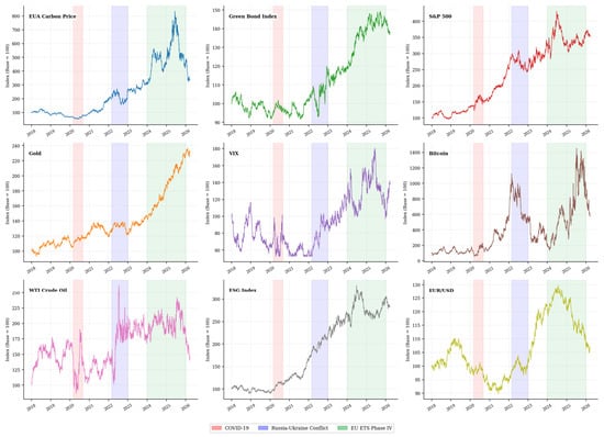
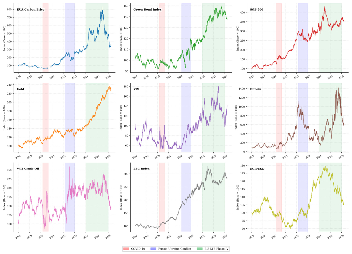
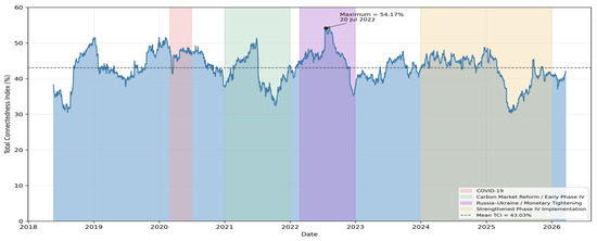
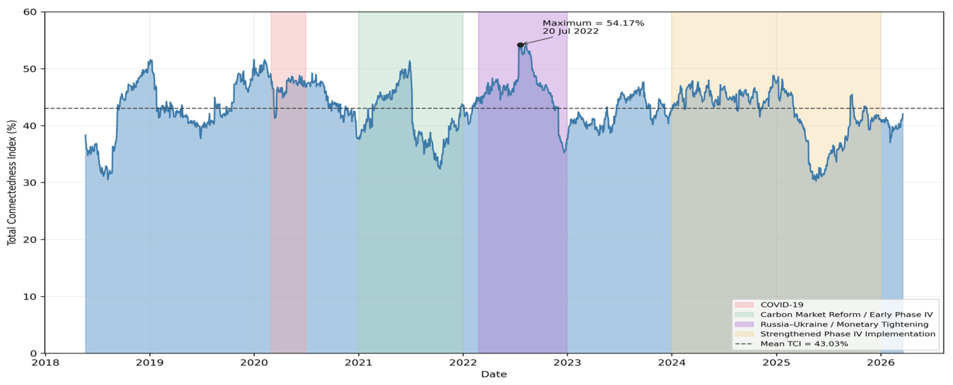
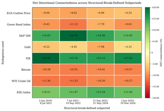
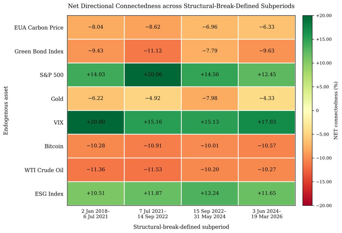
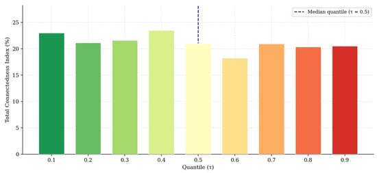
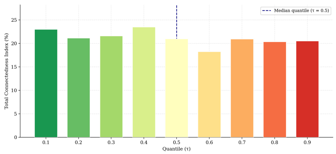
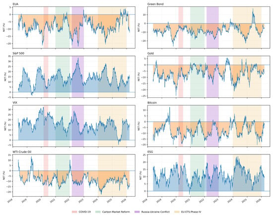
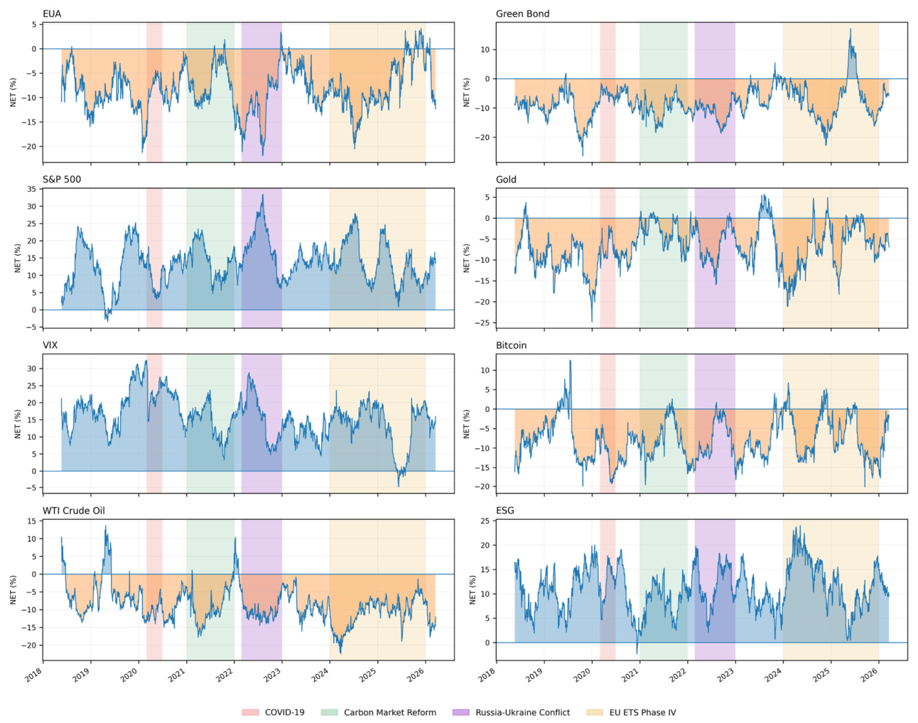
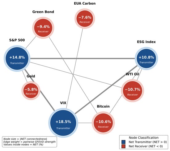
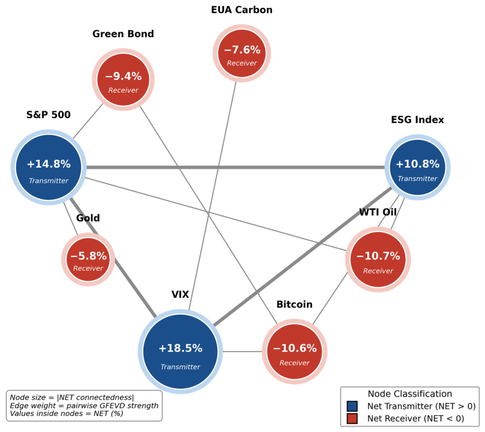

Disclaimer/Publisher’s Note: The statements, opinions and data contained in all publications are solely those of the individual author(s) and contributor(s) and not of MDPI and/or the editor(s). MDPI and/or the editor(s) disclaim responsibility for any injury to people or property resulting from any ideas, methods, instructions or products referred to in the content. |
© 2026 by the authors. Licensee MDPI, Basel, Switzerland. This article is an open access article distributed under the terms and conditions of the Creative Commons Attribution (CC BY) license.