


Abstract
This paper develops a queueing-organized framework for within-venue monitoring of BTC/USDT liquidity, signed-flow pressure, and resiliency on Binance. The model treats latent buy and sell pressure as occupancy processes and organizes three empirical diagnostics: the variance-per-BTC liquidity measure , the mean-reversion rate , and the companion signed-flow proxy . Using Binance trade data from 2020–2025, the empirical results show a pooled first-order variance–volume regularity away from the highest-volume tail, material rolling variation in liquidity and resiliency, and stronger next-day risk sorting from rolling than from Amihud illiquidity or a Kyle-style minute-impact benchmark. In overlapping 30-day windows, is positive by point estimate in roughly two-thirds of windows but clearly positive in only about two-fifths under a simple uncertainty buffer, implying that local recovery is often fragile or ambiguous. The one-hour symmetric benchmark is useful as a coarse center benchmark, but the heaviest tails require a Student-t VaR overlay. The framework is intended for risk managers, execution desks, market makers, and exchange surveillance teams that need indicators of thinning liquidity, weakening recovery, and one-sided signed flow. Queueing is useful because it turns those signals into one monitoring dashboard for market quality and short-horizon risk.
1. Introduction
Binance spot BTC/USDT is a useful venue for studying short-horizon liquidity and resiliency because it combines continuous high-turnover trading with auditable trade prints and aggressor-side information. Those features support venue-level diagnostics built directly from transaction data and make it possible to track how trading activity, signed flow, and recovery conditions evolve through time inside a single market.
This paper develops a queueing-organized monitoring framework for three linked objects: the variance-per-BTC liquidity diagnostic , the effective mean-reversion rate , and the companion signed-flow proxy . The queueing layer models latent buy and sell pressure as occupancy processes. Customer-level queues are not directly observed, but this state-space view places liquidity, signed-flow pressure, and recovery on one common stock-flow accounting system instead of treating them as unrelated reduced-form measures. The practical question is simple: when do trade prints suggest that this venue is liquid and resilient, and when do they instead suggest that it is becoming thin, one-sided, and fragile?
The paper sits at the intersection of four areas in the literature: queueing and inventory-based market models (Cont & de Larrard, 2013; Garriott et al., 2025), order-flow and price-impact models (Amihud & Mendelson, 1980; Ho & Stoll, 1981; Kim & Stoll, 2014; Kyle, 1985; Stoll, 1978), cryptocurrency market microstructure (Alexander et al., 2023; Anastasopoulos et al., 2026; Dimpfl, 2017), and short-horizon market-risk monitoring (Foucault et al., 2013). The contribution is a transparent single-venue monitoring framework for a continuously traded and fully auditable market, together with a direct comparison showing that its main liquidity diagnostic is related to, but not redundant with, feasible standard trade-based benchmarks.
- Who should care and why?
The natural audience includes market makers adjusting inventory, execution desks assessing trading conditions, exchange risk and surveillance teams watching for one-sided markets, and researchers who want auditable market-quality measures. What matters to those users is whether the venue is becoming thin, whether directional pressure is unwinding quickly or only weakly, and whether stressed states are followed by worse near-term risk conditions. The aim is to show that a simple queueing state space can organize those questions using observables that are available in Binance trade data.
The framework models latent buy-pressure and sell-pressure queues as two independent systems. New directional pressure arrives stochastically, existing pressure unwinds after random holding times, and the resulting net imbalance is mapped into price changes through a linear imbalance-to-price mapping. Throughout the paper, “long” and “short” label latent directional pressure rather than directly observed leveraged financing positions, and the queues should be read as BTC-normalized latent occupancy units rather than as observed limit-order-book queues. These primitives yield a stationary Skellam distribution for net inventory, a variance–volume relation, and a local feedback extension that motivates the observable monitoring diagnostics used below.
Empirically, three results largely underpin this paper. First, variance per traded BTC shows a pooled first-order regularity across volume bins, strongest away from the highest-volume tail, and the rolling series shows that liquidity conditions move materially over time. Second, lagged hourly return autocorrelation yields a rolling effective mean-reversion estimate whose point estimate is positive in roughly two-thirds of 30-day windows but clearly positive in only about two-fifths under a simple uncertainty buffer. Third, the rolling diagnostics are not only contemporaneous summaries: high- days are followed by worse next-day variance and tail outcomes than low- days, non-positive resiliency windows are followed by worse next-day tail outcomes than clearly mean-reverting ones, and rolling sorts those outcomes more sharply than rolling Amihud illiquidity or a closely matched Kyle-style minute-impact benchmark. The appendix recovery event study points in the same direction for large isolated hourly shocks.
- What is genuinely learned from queueing here?
Queueing earns its place here for three reasons. First, it makes , , and measurements on one common stock-flow state space rather than three separate alarms. Second, it gives a recovery-timescale interpretation in terms of latent pressure unwinding. Third, under the symmetric special case it supplies one concrete turnover-versus-recovery translation. The empirical core remains observable: and are directly estimated, and is a companion proxy. The one-hour symmetry-based translations are kept for interpretation rather than presented as stand-alone structural estimates. For the intended audience, the payoff is that the same framework answers three operational questions at once: how much liquidity the venue is delivering per traded BTC, how quickly it appears to recover from directional pressure, and whether signed flow is becoming one-sided enough to treat current conditions as more fragile.
Table 1 makes that added value concrete. The queueing layer does not replace reduced-form evidence; it organizes that evidence and tells the reader how the main diagnostics fit together.
Table 1.
The table shows what the queueing layer adds beyond reduced-form monitoring. The table reports the observable objects used in the main paper and the queueing interpretation attached to them.
The layered assumption stack is summarized once in Table A1. The empirical discipline is simple: and are directly estimated from hourly variance, volume, and lag-1 autocorrelation; is a companion splice built from minute directional impact and one-hour signed BTC flow; and symmetry-based quantities such as , , and are reported in the appendix as contingent arithmetic. The empirical case for the paper therefore rests on three observable margins: a pooled variance-per-BTC regularity, a rolling resiliency classification built from , and a companion signed-flow measure that helps organize market phases. The symmetric one-hour increment benchmark is a coarse center check, and the heaviest tails require the Student-t mixture overlay reported in Appendix E. A full-sample contingent queueing illustration still helps interpretation: under the nearby symmetric one-hour splices reported in Appendix B.4, the observed liquidity and resiliency bundle maps to indicative mean holding times of about 5.20–7.63 h and total latent occupancy of about 8524–12,510 BTC-normalized units.
- Scope and limitations
This is a focused single-venue paper. It is implemented on Binance spot BTC/USDT, uses a linear impact approximation, and does not run an exhaustive comparison with alternative microstructure models. Those choices are deliberate: they keep the framework transparent, auditable, and easy to implement on continuously updated trade data. The paper should therefore be read as a venue-level monitoring contribution. The central question is whether the observable diagnostics—, , and —remain jointly interpretable and practically useful inside one bookkeeping system.
Table 2 summarizes the main outputs of the framework and their empirical implementation. Section 2 presents the queueing-theoretic framework, the feedback mechanism, the data, and the empirical implementation. Section 3 reports the main results, including variance–volume evidence, directional impact triangulation, distributional fit, rolling stability, and a brief pragmatic tail-risk overlay. Section 4 discusses the implications for short-horizon price formation, liquidity, and market monitoring. Section 5 concludes.
Table 2.
Baseline monitoring dashboard for the main paper (BTC/USDT, Binance, 2020–2025). The table emphasizes directly estimated quantities and one companion proxy used in the paper’s main claims.
Additional derivations, extensions, and robustness checks are reported in the appendix.
2. Materials and Methods
2.1. Core Assumptions and Notation
- (M1)
- Independent Poisson arrivals of long () and short () latent occupancy units, BTC-normalized by bookkeeping convention.
- (M2)
- I.i.d. holding times with finite means ( queues).
- (M3)
- Linear imbalance-to-price mapping with .
All subsequent sections build directly on these three postulates. In the present trade-print dataset they are used as organizing modeling assumptions rather than as separately identified latent facts. Appendix B.5 and Appendix B.6 sketch nonlinear and finite-depth alternatives to (M3); the main text keeps the linear form because it is the clearest implementation of the monitoring system.
2.1.1. Notation and Scale Conventions
Table 3 collects the core symbols and dimensions used throughout the paper. Throughout, denotes the observable returns-scale variance-per-BTC moment computed from one-hour return increments and one-hour traded BTC volume, and its associated variance scale. The structural return-impact slope is , with units ; once the one-hour holding-time correction is introduced below, the symmetry-based special-case translation is . Price-scale variance-per-BTC is . Numerical illustrations in USD set ; all calibrations and tests use returns units, so no reported estimate depends on the choice of . For empirical bookkeeping, queue occupancies are BTC-normalized latent occupancy units throughout: one latent unit corresponds by normalization to 1 BTC. This is a bookkeeping convention for the latent state, not a claim that literal customer orders are observed in exact 1-BTC blocks. A marked or compound-Poisson generalization with random chunk sizes would be the natural extension, but the present paper uses unit-normalized occupancies to keep the monitoring diagnostics tractable. Operationally, the latent state is tied to executed BTC turnover only at the first-moment level: the normalization is chosen so that expected openings and closures of latent occupancy units match expected executed BTC volume in the bookkeeping identity used below. A marked extension would preserve that first-moment bridge while changing higher moments and tail behavior. The stationary occupancy law is the general result; the one-hour increment bridge used later for contingent structural translation is the narrower symmetric special case.
Table 3.
Core symbols and dimensions.
2.1.2. Queueing Mapping
Queueing notation treats latent occupancy-unit openings as arrivals and holding times as service; for an queue the steady-state occupancy is Poisson with mean , yielding a Skellam distribution for the long–short difference. A brief primer and the mapping from queueing language to trading pressure are provided in Appendix A.
2.2. Queueing-Theoretic Framework
2.2.1. Model Setup and Intuition
The central modeling idea is to treat the market as a system of queues in which price pressure emerges from the imbalance between outstanding long and short latent occupancy units.
Consider a Bitcoin market populated by two latent directional-pressure types: those contributing buy pressure (“longs”) and those contributing sell pressure (“shorts”). At any point in time, there are outstanding long-side occupancy units and outstanding short-side occupancy units. These are not directly observed financing books; they are state variables summarizing net pressure that remains active in the market. The key state variable is the net inventory imbalance:
Over short horizons, local price deviations are determined by this inventory imbalance through a linear imbalance-to-price mapping:
where is a slowly moving local reference level and measures the local price effect per unit of net inventory.
Impact-Kernel Interpretation
Let latent occupancy-unit openings arrive at times with sign and holding time . Then
and, taking expectations, the mean price follows
This is a shot-noise/propagator representation of latent directional pressure with kernel G given by the holding-time survival function (Bouchaud et al., 2009). It is not a one-to-one mapping from public trade prints to literal queue openings and exits; executed BTC enters the empirical implementation only through the first-moment bookkeeping bridge in Equation (12). In this interpretation, the price effect persists while latent pressure survives and decays as occupancy exits. The mean holding time is therefore an effective resiliency timescale of latent order-flow pressure; in the present implementation that timescale is inferred from lagged hourly return autocorrelation and then translated into under symmetry (Section 2.5).
The dynamics of long and short occupancy units follow queueing processes. New long-side units arrive at rate and each unit is held for a random time drawn from distribution . Similarly, new short-side units arrive at rate with holding times drawn from . The heterogeneity in trader horizons is captured by the entire distribution of holding times rather than a single parameter.
The model is applied to Binance BTC/USDT spot transactions over the period 1 January 2020–9 July 2025. The empirical work does not directly estimate customer-level arrivals, exits, or holding times from minute buckets, nor does it observe order-book queue position. Instead, it estimates an observable variance scale, a minute directional-impact proxy, and an effective mean-reversion rate, then translates those objects into contingent structural quantities under symmetry for interpretation. Data conventions and empirical estimates are reported in Section 2.4 and Section 3.
These assumptions are most appropriate when trading is continuous, turnover is high, and short-horizon price adjustment is strongly influenced by order flow; BTC/USDT fits those conditions reasonably well over the sample horizon (see Appendix A).
2.2.2. Stationary Inventories and Skellam Law
Outstanding long and short occupancy units each follow an queueing system. New units arrive according to Poisson processes with rates and , and holding times are drawn from and with means and .
A standard queueing result is Palm’s theorem (Palm, 1943), which characterizes the steady-state distribution of an system:
Lemma 1
(Palm’s Theorem). In an queueing system with arrival rate λ and service time distribution with mean , the steady-state occupancy is Poisson distributed with parameter .
Applied to this setting, steady-state occupancies are
with and .
Under the maintained baseline specification, the long and short queues are independent even though they operate in the same market. This independence is imposed through independent Poisson arrivals and independent holding periods across traders.
The steady-state net inventory is therefore
This stationary result should be read as a local law for price deviations around the reference level , not as a literal unconditional law for the full Bitcoin price path over 2020–2025. The Skellam distribution—previously applied to tick-level price changes by Koopman et al. (2017)—emerges here as the stationary distribution of net inventory from explicit queueing primitives, linking arrival rates and holding times directly to local price-deviation moments.
Illustrative symmetry-based translations for and the associated Skellam parameters are reported only in Appendix B.3.
2.2.3. Price Distribution and Over-Dispersion
The Skellam distribution has probability mass function:
where is the modified Bessel function of the first kind of order n.1
From Equation (2), the local price-deviation distribution is:
All moments of the local price-deviation distribution are available in closed form:
These formulas reveal several important insights.
- (i)
- First, the expected local price deviation is proportional to the difference between long and short pressure , formalizing the sign of the local price effect from net order imbalance.
- (ii)
- Second, local price-deviation volatility scales with the sum of these pressures , so intense activity on either side widens the stationary distribution of price deviations.
- (iii)
- Third, under the baseline Poisson specification the excess kurtosis iswhich vanishes as order-flow intensity grows, implying asymptotically normal tails.
Empirically, hourly returns display extreme excess kurtosis (≈47.29), while the hourly buy-count and sell-count series are strongly over-dispersed relative to a Poisson benchmark. Fitting Gamma-mixed Poisson models to the hourly count series gives full-sample dispersion parameters and . These are trade-count burstiness proxies rather than BTC-commensurate structural calibrations of the latent queues, so the count-space extension below is retained only as a supplementary burstiness benchmark.
2.2.4. Negative–Binomial Over-Dispersion
Observed hourly buy and sell trade counts are substantially more bursty than a pure Poisson benchmark. To document that without overloading the main paper, a Gamma-mixed Poisson extension is used only as a count-space burstiness proxy. Under a common-rate approximation for the buy and sell count mixtures, the hourly increment’s excess kurtosis can be decomposed into a tiny Poisson benchmark term plus a much larger over-dispersion term. For Binance, the Poisson term is only while the over-dispersion contribution is , which is why the paper treats burstiness as a real feature of the count data. The exact common-rate derivation and parameterization are deferred to Appendix H; in the main paper this point is only supplementary and does not change the interpretation of the core liquidity and resiliency diagnostics.
2.2.5. Variance–Volume Relation
At the first-moment level, the queueing framework implies a disciplined link between trading volume and the ex ante variance in price changes. Under the BTC-normalized latent-unit convention, observed executed BTC volume is bookkept by expected openings and expected closures of latent occupancy units. No event-level one-to-one mapping from public trades to literal latent queue openings or closures is being claimed. Because each side of the book is an queue with mean inventory and exit rate , the BTC-normalized first-moment bookkeeping rate for executed volume is
where the first term captures arrivals and the second departures. The last equality follows by substituting . Under this normalization, each latent occupancy unit contributes one BTC when opened and one BTC when closed in the first-moment bookkeeping. Equation (12) is a bookkeeping identity under the BTC-normalized latent-unit convention, not direct observation of literal queue openings and closures. The model therefore does not independently predict venue volume. Instead, it uses a BTC-normalized first-moment convention to place observed turnover and latent occupancy on a common scale. The paper’s falsifiable content begins at the observable level: the variance-per-BTC moment , the effective mean-reversion estimate , the proxy feedback diagnostic , and the success or failure of the symmetric increment benchmarks. It does not begin at literal queue openings or at the contingent symmetry translations reported later only for interpretation.
Sample Mean Executed Volume
Given the hour-by-hour executed BTC volume , the long-run mean hourly executed BTC volume is estimated by
where T is the number of hourly bars in the sample.
Empirical Calibration
Section 3.2 reports the empirical estimates of , its square-root scale , and the contingent structural translation for Binance BTC/USDT. Table 2 summarizes the main outputs.
Returns form (used in all calibrations and Q–Q plots): with and ,
2.3. Feedback, Stability, and Resiliency Mechanism
At intraday horizons, signed-flow intensities can respond to recent price movements. This extension adds a local state-dependent splice to motivate a proxy-based resiliency classifier within the queueing framework. In the empirical sections below, the object carried forward is the local pair , not a claim of direct structural estimation of the latent queue-stability boundary.
2.3.1. State-Dependent Arrivals
The model is extended to allow arrival rates that depend on recent price changes, capturing local return-following or contrarian signed-flow behavior in a latent queueing splice.
Standing Assumptions
- A1
- (Queueing) Arrivals of long- and short-side latent occupancy units are independent Poisson with baseline rates ; holding times are independent and identically distributed (i.i.d.) with finite means .
- A2
- (Linear price impact) Price obeys with constant .
- A3
Linear Feedback Specification
Let denote the aggregate exit intensity [] and define the rescaled latent feedback coefficient
To avoid confusion with observed close-to-close one-hour return increments, let
denote the model’s local latent price-deviation state in returns units. The feedback equations in this subsection are written in terms of , whereas the empirical sections reserve for observed one-hour close-to-close returns and estimate the separate proxy coefficient from lagged returns and signed BTC flow. Let arrival rates respond linearly to the recent (left-limit) local price-deviation state :
where are baseline arrival rates and measures the strength of state dependence in the latent price-deviation state. When , positive recent deviations are associated with return-following latent pressure; when , positive deviations are associated with contrarian latent pressure. Because is -measurable, this specification is predictable and introduces no simultaneity. Equations (14) and (15) are interpreted as a local linearisation, with rates truncated at zero if needed; under the full-sample symmetry translation summarized in Appendix B.3, the implied perturbation is small relative to the baseline intensities , so truncation does not bind in practice.
Linearized Dynamics
For the local OU approximation in this subsection, symmetric exits are additionally imposed. Substituting into the net arrival rate gives feedback proportional to , so the drift of the expected net inventory is
Whenever the local effective mean-reversion rate
is positive, the corresponding local mean level is
Defining the centered state , the local linearized dynamics take the Ornstein–Uhlenbeck form
where is the baseline event intensity and is a standard Wiener process. The continuous-time stability condition is therefore
Stability Analysis
The centered local linearization is mean-reverting only when the drift coefficient is positive, i.e., when , equivalently under the symmetric-exit splice. This inequality is best read as a latent heuristic for the sign logic behind the observed pair rather than as a directly identified latent stability boundary. Baseline asymmetry shifts the local mean level but does not by itself change that local sign condition. Empirically, the paper uses this splice only to organize local regime classification through and the companion proxy ; the corresponding contingent symmetry summary for is reported only in Appendix C.10.
Metrics
The implied resiliency half-life—the time for the centered state to decay halfway back toward its local mean after a shock—is , where is the effective mean-reversion rate from (18). Because the structural is not directly observed, the main text focuses on the directly estimated pair and treats any further translation into , , , or as contingent on the symmetric proxy mapping summarized only in the appendix. For the calibrated parameters (Table 4), this yields the descriptive full-sample contingent illustration h. The empirical role of this subsection is therefore local and fragile by design: it supplies a queueing-organized interpretation for observed resiliency diagnostics, not a claim that the latent queue boundary is directly estimated from venue data.
Table 4.
Technical pooled-baseline input table for the main empirical implementation (BTC/USDT, Binance, 2020–2025). Table 2 is the baseline monitoring dashboard; this table records the directly estimated and proxy-based ingredients behind it.
2.4. Data
The empirical implementation uses Binance BTC/USDT trade data from 1 January 2020 through 9 July 2025, a window that spans the 2021 bull market, the FTX collapse, and the 2024 exchange-traded fund (ETF) launch period. The working sample contains 48,374 hourly bars over 2017 Coordinated Universal Time (UTC) days. A complete UTC grid over that span would contain 48,408 h; the realized panel contains 48,374 because 34 h are missing on 15 UTC days. Those missing hours come from gaps in the source hourly summary files that feed the canonical hourly panel, not from discretionary filtering or from the later aggressor-side merge. The analysis retains those partial UTC days and computes daily variance and volume from the observed hourly bars. Dropping the 15 incomplete UTC days changes the headline variance-per-BTC estimate by less than 1% and leaves the lag-1 return autocorrelation essentially unchanged, so the main results are not driven by those omissions. For each UTC day, the workflow uses the raw tick file to construct minute-level signed BTC flow and returns, the workflow-generated hourly summary file for close-to-close returns and traded BTC volume, and the workflow-generated aggressor-side summary file to build an hourly panel of buyer-initiated BTC volume. All timestamps are converted to UTC. Binance spot BTC/USDT is used as a first venue because it combines deep continuous trading with directly auditable trade-print and aggressor-side records, which makes it a practical setting for a queueing-based monitoring exercise even though the broader Bitcoin market is multi-venue.
All data processing, estimation, figure generation, and Monte Carlo validation were performed in Python 3.9.6 using NumPy 1.26.4, SciPy 1.13.1, pandas 2.2.2, and matplotlib 3.9.4. full Python code that produces these results is provided as Supplementary Materials.
The empirical pipeline therefore uses three aligned objects: an hourly return/volume panel, a day-level minute-regression panel, and an hourly signed-BTC-flow panel. The first supports the variance–volume and mean-reversion estimates, the second provides a directional-impact scale in BTC units, and the third provides the signed-flow input for the feedback and rolling-diagnostic results.
Sign convention. Signed order flow uses the taker side: a trade has sign if the aggressor is the buyer and if the aggressor is the seller. Concretely, the convention takes isBuyerMaker=False as and True as . Buyer-initiated and seller-initiated BTC volume are therefore observed directly at the trade level and then aggregated to minute or hourly frequency as needed.
Cleaning and alignment. The construction is deliberately mechanical. The canonical hourly panel retains only rows with finite hourly close, traded BTC volume, and close-to-close return values, then sorts by UTC timestamp. In the minute regressions, raw trade records with non-finite price, quantity, or timestamp fields are dropped, timestamps are normalized to milliseconds, and signed BTC flow is aggregated within exact UTC minutes before minute returns are computed from the first and last trade in each occupied minute. The hourly BTC-flow panel is then matched hour-by-hour to the workflow-generated aggressor-side summary files; the workflow stops if any required day is missing or if the merge produces missing hourly buy quantities. No manual winsorization or discretionary outlier deletion is applied in these steps.
2.5. Empirical Implementation
The framework is implemented at the one-hour horizon unless stated otherwise. The empirical procedure distinguishes four objects. First, is an observable variance scale identified from the variance–volume moment condition. Second, is an effective mean-reversion rate identified from return autocorrelation. Third, is a minute directional-impact slope in BTC units. Fourth, is a proxy-based feedback rate obtained by combining with one-hour signed BTC flow. Structural quantities such as , , , , and are reported only as model-implied translations under the symmetry mapping. Throughout this section, all bar-level observables are one-hour totals: price-scale variance satisfies and returns-scale variance satisfies .
2.5.1. Observable Variance Scale
The variance–volume identity yields the one-hour variance scale
This is an observable variance coefficient, not a directional-impact slope. Standard errors are computed with a block bootstrap using 10,000 resamples of 24 h blocks.
2.5.2. Effective Mean-Reversion
The aggregate mean-reversion rate is identified from the lag-1 autocorrelation of hourly returns. Under the OU linearisation (18), the lag-1 autocorrelation coefficient satisfies . The estimate is
which follows because the lag-1 autocorrelation of the OU increment is , and is well-defined when , i.e., . Applied to simple hourly returns, this is a local short-horizon approximation rather than an exact identity for the full return process. The resiliency half-life follows as , and the structural exit rate is implied under the proxy mapping as . Because is identified from a single autocorrelation coefficient (SE ), the half-life is imprecisely estimated; a two-standard-error band spans roughly 10–25 h.
2.5.3. Directional-Impact Scale
To obtain a unit-consistent flow-feedback diagnostic, the implementation first estimates day-by-day minute regressions of one-minute returns on contemporaneous signed BTC flow:
where is signed BTC volume (buyer-initiated minus seller-initiated) computed directly from trade records. The directional-impact scale used in the feedback mapping is
This scale has units and is reported descriptively in Section 3.3. The day intercepts are estimated but not interpreted.
2.5.4. Feedback
Hourly signed BTC flow is then constructed from buyer-initiated minus seller-initiated BTC volume, and the estimated regression is
where is measured in BTC within hour t, so has units BTC per unit return. A short discrete-time bridge makes the sign-and-units convention explicit. Let h and define the excess signed flow over hour t by
where the second step is the local left-endpoint approximation under (14) and (15). Using the lagged one-hour return as the empirical proxy for the local deviation and as the minute-scale BTC-to-return slope proxy gives
With h, this reduces to (23). This bridge is used only as a latent sign-and-units heuristic. Because is an observed increment proxy for the unobserved latent state rather than the state itself, the resulting object is reported as , not as a direct estimate of the structural quantity and not as a mapped latent feedback rate. The minute/hour splice is a deliberate technical compromise: minute regressions stabilize the directional-impact slope, whereas hourly aggregation yields a less noisy signed-BTC-flow slope. That choice is useful for extracting a directional monitoring signal, but it leaves the absolute proxy level splice-sensitive; nearby-frequency robustness is reported in Appendix C.9. In the rolling 30-day results below, the signed-flow slope is re-estimated within each rolling window and combined with the same-window rolling median of daily directional-impact slopes, with the observed missing UTC hours carried through the hourly grid rather than filled. When the flow is contrarian; when it is return-following.
2.5.5. Workflow and Units
The proxy construction is intentionally mechanical. Step 1: estimate the minute directional scale in units . Step 2: estimate the hourly signed-flow slope in units BTC per unit return. Step 3: apply the one-hour discrete approximation above so that is an hourly signed-flow monitoring proxy in . This makes the splice transparent, but it does not turn into a directly identified arrival-rate parameter.
2.5.6. Model-Implied Structural Translation
Under the symmetric special-case translation used for interpretation, the structural holding time is . For one-hour return increments, Appendix B.2 shows that the holding-time correction factor is
so the structural return-impact slope follows as . This bridge is exact for the symmetric exponential-holding-time mapping; it is not a nonparametric identification result. Additional occupancy translations, including and under the same symmetry calibration, are reported only in Appendix B.3. All such quantities are reported as contingent model translations for interpretation, not as directly estimated facts.
A related distinction matters for the empirical results below. The stationary Skellam law from Section 2.2.2 concerns the level of latent imbalance , whereas the distributional diagnostics in Section 3.4 benchmark one-hour return increments generated from that same core.
3. Results
3.1. Main Parameter Estimates
The empirical quantities are estimated as described in Section 2.5. See Appendix F for a Monte Carlo confirmation that the variance-scale estimator based on is effectively unbiased in finite samples.
The empirical mapping uses three observables: variance per traded BTC for , lag-1 hourly return autocorrelation for , and the pair for . These are the main empirical objects; any further translation into , , , , or is reported only in the appendix and remains contingent on the symmetric bridge. Table 4 records the headline inputs. The full-sample values are , , implying a descriptive half-life of 14.54 h, and baseline-splice . Nearby-frequency alternatives, and , show that the proxy sign is stable while the exact level is splice-sensitive. Additional tail and supplementary diagnostics are reported in Appendix C. Public OHLCV aggregates are not used for calibration because the implementation relies on trade-print volume and aggressor-side information; brief reconciliation notes appear in Appendix D.
3.2. Variance–Volume Evidence
Figure 1 is a visual summary of the empirical relationship between within-day variance and daily trading volume. The grouped scatter averages days within rounded daily volume-percentile bins labeled , so the two endpoint bins contain 101 days each and the interior bins contain about 201–202 days each. Within-day variance is computed from hourly close-to-close simple returns within each day; daily volume is total executed BTC volume that day. Log returns are not used anywhere in this test. The heavier evidentiary work comes from the day-level ratio contrast below, the compact grouped-slope companion, and the within-bin dispersion evidence in Appendix C.1. Because that grouped-slope companion is built from daily observations rather than hourly bars, its uncertainty uses a 7-day moving-block bootstrap rather than the 24 h block bootstrap used for the hourly variance coefficient.
Figure 1.
Variance–volume evidence for BTC/USDT, 2020–2025. The (left) panel shows within-day variance in simple hourly returns against same-day executed BTC volume; gray points are daily observations and blue points are grouped averages formed from rounded daily volume-percentile bins over the 2017 UTC trading days in the sample. The (right) panel reports the within-bin daily variance-per-BTC ratio with median and interquartile range by volume bin. The main takeaway is a pooled first-order rise of variance with volume together with a more stable middle-bin ratio pattern and visible attenuation only in the highest-volume endpoint bin.
The visual deviation in Figure 1 is concentrated in the high-volume tail. In the grouped scatter, the highest-volume endpoint bin is visibly attenuated; in a separate day-level contrast, the mean daily ratio in the top 10% of days is only 0.569 times the corresponding ratio in the middle 60% of days. A compact quantitative companion (Table 5) gives the same message: excluding the highest-volume endpoint bin, the grouped n-weighted through-origin slope is with 95% block-bootstrap interval [, ], versus the theoretical slope . The qualitative message is unchanged if all grouped bins are retained () or if the top two bins are excluded (), which is why the endpoint exclusion is best read as a transparent display choice rather than an after-the-fact search for significance. The variance–volume evidence is therefore used as a descriptive first-order compatibility check rather than as a sharp invariance test. Appendix C.1 reports the within-bin dispersion of the daily variance-per-BTC ratio across volume bins, and Table 6 shows that the reduced-form moment also shifts across broad sub-periods. Taken together, those checks support a pooled liquidity-monitoring regularity rather than a time-invariant liquidity law.
Table 5.
Compact quantitative companion to the variance–volume figure. The grouped slope excludes only the highest-volume endpoint bin and uses a 7-day moving-block bootstrap.
Table 6.
Broad sub-sample reduced-form checks. Including the intermediate 2023 phase shows directly that the reduced-form liquidity and resiliency moments move across major market phases, which is why the paper treats as a pooled first-order diagnostic rather than as a constant law. Hours are reported so the pooled baseline benchmarks are not read as stable venue constants. Each sub-period estimate is computed from the same pooled formulas used for the full-sample benchmarks, restricted only to observations inside that sub-period.
Figure 2 makes that liquidity movement visible at the same rolling horizon used later for the resiliency diagnostics. The rolling series is noisier than the pooled estimate, but it confirms that the liquidity moment itself is time-varying rather than merely a full-sample summary. The paper therefore treats as a monitorable liquidity diagnostic whose pooled estimate remains useful for benchmarking, not as a constant law of the venue. In the daily variance–volume scatter, each day d has x-coordinate equal to total daily BTC volume and y-coordinate equal to the within-day sample variance in hourly returns. Since while , the model’s variance–volume identity implies a predicted slope
With the full-sample moments in Table 4, this yields a predicted daily scatter slope of . Empirically, the day-by-day ratios have mean , which is the primary estimate under the constant-ratio hypothesis. The day-level OLS slope through the origin is lower at because it effectively volume-weights. High-volume days exhibit attenuated ratios when gross two-sided trading rises faster than the net directional pressure that drives prices. That gross-versus-net reading is plausible, but it should be treated as an interpretation of the attenuation rather than as a separately established result. This attenuation is especially pronounced in the highest-volume endpoint bin (mean BTC/day, days). In the median-based right panel of Figure 1, the endpoint-bin median is only about 14% of the overall mean ratio; at the day-level mean ratio, the same endpoint bin averages about times the overall mean. One plausible reading is that gross two-sided activity rises faster than net directional pressure on those days, but the paper treats that only as an interpretation of the attenuation rather than as a separate empirical result. The fitted reference line in Figure 1 uses the theoretical slope ; the empirical OLS-through-origin slope is overlaid as a secondary comparison.
Figure 2.
Rolling 30-day estimate of the one-hour variance-per-BTC moment for BTC/USDT, sampled once per UTC day. The line is computed from hourly returns and hourly executed BTC volume inside each trailing 30-day window, and the dashed line marks the full-sample estimate. The main takeaway is that the liquidity diagnostic itself moves over time, so the paper’s monitoring interpretation is explicitly dynamic rather than purely pooled.
3.3. Directional Impact Cross-Check
As an independent empirical cross-check on price impact, the analysis uses day-by-day minute signed-flow regressions only as descriptive triangulation and as a normalization device for the feedback proxy, not as a causal impact design or as structural identification. The day-by-day minute-level regressions relate one-minute returns to contemporaneous signed BTC order flow. For each day d, the regression is
where is signed BTC volume (buyer-initiated minus seller-initiated) computed directly from trade records as , with qty the Binance base-asset quantity in BTC and indicating trade direction; hence has units . The daily intercept is estimated but not used elsewhere in the paper. Across 2017 days, the median is with interquartile range , and the median is . The absolute-median summary is used only to obtain a positive directional-impact scale for the feedback proxy. In the present sample this choice is not driving the result mechanically: the median signed slope is also , and negative daily slopes occur on fewer than 0.05% of days. These minute-level slopes are about smaller than the observable variance scale , which is expected because is a variance coefficient while is a directional slope in BTC units. The moderate median of suggests that minute signed flow carries economically meaningful price information, but the regression is used only to supply the directional normalization in . The separate variance–volume moment condition provides the variance-consistent scale used in the diffusion calculations.
3.4. Variance-Matched One-Hour Skellam Benchmark and Falsification Check
This subsection is intentionally a falsification check rather than a validation exercise. Figure 3 compares empirical hourly returns to a variance-matched one-hour Skellam benchmark. The object benchmarked here is not the exact increment law of the general framework. Rather, it is the symmetric special-case reference distribution obtained after fixing the one-hour horizon, replacing realized volume by the sample mean one-hour BTC volume, and matching the observed one-hour variance scale . This benchmark intentionally switches off feedback and regime variation so the symmetric core can be judged on its own. Specifically, the theoretical quantiles are generated from
where is the sample mean hourly return and is the sample mean hourly traded BTC volume. Figure 3 therefore benchmarks one-hour return increments under a symmetric variance-matched reference distribution; it does not fit the stationary price-level law from Section 2.2.2 directly, and it should be read as an unconditional benchmark rather than as a fully volume-conditioned fit. Sharper evidence appears in Table 7, which conditions on realized one-hour volume. After standardizing returns by , the model-implied central 80% and 50% bands cover 85.3% and 60.7% of standardized observations, with empirical/model width ratios 0.862 and 0.756. Ratios below one mean that the model-implied central bands are wider than the empirical center. These results reject the symmetric benchmark as a full descriptive model for hourly spot BTC/USDT returns, but that does not make the framework useless: the practical value of the paper lies in monitoring liquidity per traded BTC, local recovery timescales, and signed-flow pressure, while the benchmark still serves as a transparent center-of-distribution reference that shows exactly where an additional tail overlay is needed. Additional burstiness and tail diagnostics are deferred to Appendix C.2 and Appendix C.4.
Figure 3.
Q–Q comparison of empirical hourly BTC simple returns with a variance-matched Skellam benchmark. Blue circles are empirical sample quantiles plotted against the variance-matched Skellam theoretical quantiles; the dashed line is the 45-degree reference indicating perfect agreement with the Skellam benchmark. The symmetric reference provides only a coarse description of the center and understates the most extreme moves. Table 7 contains the sharper evidence after conditioning on realized one-hour volume.
Table 7.
Volume-conditioned middle-quantile check for standardized one-hour returns. Conditioning on realized one-hour BTC volume improves the center-fit comparison relative to the unconditional Q–Q benchmark, but the symmetric core still remains too dispersed. Width ratios below one imply that the model-implied central bands are wider than the empirical center.
Even after conditioning on realized one-hour volume, the single-regime symmetric core remains too wide in the center and too thin in the far tails. Appendices Appendix C.2 and Appendix C.4 report the supplementary burstiness and tail diagnostics.
3.5. Rolling Regime Classification Under the Proxy Mapping
The full-sample one-hour signed-BTC-flow slope is , and combining it with the directional-impact scale yields a positive companion signed-flow proxy of baseline-splice with propagated 95% interval . The interval construction is simulation-based: 200,000 draws combine a HAC-normal approximation for with the bootstrap distribution of , so it should be read as sampling uncertainty conditional on the baseline splice. The effective mean-reversion rate remains positive at , with interval , implying a descriptive full-sample resiliency half-life of 14.54 h. A positive by itself does not imply instability: under the local OU splice, the key question is whether mean reversion remains strong enough for to stay positive. Nearby-frequency checks leave the sign intact but move the point estimate to and , so the broad practical range across the baseline and nearby alternatives is closer to than to the conditional propagated interval alone. In that sense, the sign of is more credible than its exact level. The nearby-frequency checks are therefore used only to show that the splice is not sign-fragile; they do not convert into a directly identified structural parameter. Any summary remains secondary and is left to the appendix.
Rolling estimation sharpens that interpretation. The rolling analysis uses overlapping 30-day windows as a compromise between local stationarity and enough hourly observations to estimate the return autocorrelation and signed-flow slope without excessive noise. After the initial window-fill period, this yields 47,655 non-missing 30-day window estimates.2 In the baseline overlapping 30-day scheme, 66.2% of windows have by point estimate alone. That point-sign share is informative but too optimistic to stand on its own. Using a simple one-standard-error autocorrelation buffer of around zero, 39.2% of overlapping 30-day windows are clearly mean-reverting, 49.4% are ambiguous, and 11.5% are non-positive. This buffer is a heuristic monitoring rule rather than a formal confidence interval under heteroskedastic, serially dependent returns. A more conservative doubled companion buffer leaves only 17.2% of overlapping windows clearly mean-reverting and 79.9% ambiguous. Across those two heuristic buffers, the clearly mean-reverting share therefore lies in a range of roughly 17.2–39.2%, with ambiguity dominant under either rule. The daily-sampled and non-overlapping companion splits are similar: (39.2%, 49.4%, 11.4%) and (38.8%, 49.3%, 11.9%). Appendix C.6 reports the full sensitivity tables, including shorter 15-day and longer 60-day windows and the conservative companion buffer. The rolling feedback proxy remains economically meaningful, but the central regime-classification result is the sign and magnitude of , not the behavior of any derived boundary ratio.
Figure 4 reports the rolling feedback and mean-reversion diagnostics. The figure should be read first as a regime-classification device based on , with the rolling feedback proxy shown alongside it. Taken together, the full-sample and rolling results are consistent with return-following signed-flow pressure in BTC/USDT, but the mean-reverting component dominates only in a subset of windows once a near-zero heuristic buffer is imposed. The windows with ambiguous or non-positive are economically important precisely because they identify periods in which the baseline queueing interpretation becomes unreliable.
Figure 4.
Rolling feedback and mean-reversion diagnostics for BTC/USDT, Binance, 2020–2025. The underlying estimates are computed in overlapping 30-day windows updated each hour after the initial 30-day fill period, but the figure samples one end-of-day point per UTC day for display clarity. Panel (a) reports the rolling companion proxy , and panel (b) reports the rolling effective mean-reversion estimate . Under the baseline heuristic buffer, the hourly-updated 30-day split is 39.2% clear positive, 49.4% ambiguous, and 11.5% non-positive. Hatched amber shading marks ambiguous windows and cross-hatched gray shading marks non-positive windows, where the local OU interpretation is not used.
3.6. Simple Next-Day Monitoring-Value Check
To check whether the rolling diagnostics do more than summarize the same-day sample, the analysis runs a deliberately simple day-ahead sort. For each UTC day d, the end-of-day 30-day rolling liquidity diagnostic is paired with the end-of-day rolling regime label from Figure 4, then compared with realized outcomes on day . The matched sample starts only once both predictors are fully filled 30-day end-of-day diagnostics. The outcomes are next-day realized variance in hourly returns, the next-day maximum absolute hourly return, and a tail-day indicator equal to one when the next-day maximum absolute hourly return falls in the top decile of the matched sample. This is not a forecast horse race and does not claim optimal monitoring thresholds; it is a descriptive check of whether the rolling outputs sort meaningfully different next-day risk conditions.
Table 8 shows that the rolling liquidity diagnostic carries the clearest next-day signal. Moving from the low to the high rolling- tercile raises next-day realized variance from 0.000026 to 0.000072, increases the next-day mean maximum absolute hourly return from 1.31% to 1.98%, and raises the next-day tail-day rate from 6.5% to 15.1%. The resiliency classification adds a weaker but directionally similar signal: non-positive windows are followed by larger next-day maximum hourly moves and higher tail-day rates than clearly mean-reverting windows (13.3% versus 8.9%). Under the doubled companion buffer from Appendix C.6, the clearly classified sample shrinks sharply (347 clear-positive days and 59 non-positive days), but the same tail-rate ordering remains directionally intact (15.3% versus 6.9%). These patterns do not validate a trading rule or establish predictive superiority over a generic volatility-persistence monitor, but they do show that the rolling diagnostics carry useful next-day monitoring information rather than functioning only as contemporaneous summaries.
Table 8.
Simple next-day monitoring-value check based on end-of-day 30-day rolling diagnostics. Predictors are measured at the end of UTC day d, and outcomes are computed from the observed hourly returns on day . The matched sample contains 1987 predictor–outcome day pairs, running from 30 January 2020 through 8 July 2025. The first 29 UTC days are omitted so that both end-of-day predictors are fully filled 30-day diagnostics, and the final sample day is omitted because it has no outcome; 15 matched days contain fewer than 24 hourly returns because of the observed missing UTC hours. “Tail day” means that the next-day maximum absolute hourly return lies in the top decile of the matched sample, with threshold 2.89%. Because the predictors are persistent rolling states, this table is included only as a descriptive relevance check and does not establish incremental forecast evidence over generic volatility persistence.
To see whether rolling is only a relabeling of familiar trade-based liquidity measures, Appendix C.8 applies the same 30-day day-ahead design to two feasible public-data benchmarks: rolling Amihud illiquidity and a rolling Kyle-style minute signed-flow impact slope. Because the Amihud series requires 30 non-missing daily return-volume pairs, that benchmark comparison begins one day later than Table 8. Rolling is positively related to both, with correlations 0.304 and 0.630, but it sorts next-day tail outcomes more sharply. The high-minus-low tail-day spread is 8.6 percentage points for rolling , versus 4.7 for rolling Amihud and 1.1 for the Kyle-style minute-impact slope. That does not make a universal winner in every application, but it does show that the queueing-organized liquidity diagnostic is not redundant with these feasible trade-based benchmarks in the same day-ahead design.
3.7. Secondary One-Hour Tail Overlay
For the empirical risk application, the analysis stays in reduced-form observable notation and at the one-hour horizon only. Let denote average one-hour BTC volume, and let denote the observed one-hour return variance. The core one-hour benchmark is therefore the Normal approximation with variance . To monitor the most extreme tail events, the analysis adds a threshold-split Normal-plus-Student-t overlay re-fit every 24 h inside trailing 2160 h windows. Over 46,214 hourly forecasts, the rolling Gaussian benchmark breaches at 1.80% and the stress-state overlay at 1.13%. That overlay is included as a supporting parametric tail monitor; fuller benchmark comparisons and backtesting details remain in Appendices Appendix E and Appendix C.11.
4. Discussion
4.1. Short-Horizon Price Formation and Liquidity Interpretation
The results support a market-microstructure interpretation in which inventory and trade imbalances shape short-horizon BTC/USDT price variation on Binance. The variance–volume relation shows that gross trading activity and short-horizon variance move together in a disciplined way. At the same time, the BTC-flow diagnostics are consistent with positive returns being followed, on average, by additional buyer-initiated BTC flow at the hourly horizon. In practical terms, this means that high activity can raise volatility through both gross two-sided trading and directional signed-flow pressure, even though full-sample return autocorrelation remains negative.
The queueing formulation is useful because, inside the model, arrival and holding-time assumptions organize occupancies, occupancies organize net imbalance, and net imbalance organizes the local price-deviation state. Empirically, the paper identifies monitoring diagnostics tied to that structure rather than the underlying queue primitives themselves. That decomposition explains what would be lost without queueing: the observable bundle would no longer live in one stock-flow state space, the recovery interpretation of would lose its turnover counterpart, and the pooled occupancy translation would disappear. The model adds value by providing a disciplined accounting system that connects observable market states to short-horizon price formation, volatility, and resiliency.
4.2. Market Monitoring and Risk Application
From a monitoring perspective, the strongest outputs are the rolling liquidity path in Figure 2, the rolling resiliency classification in Figure 4, and the next-day descriptive sort in Table 8. A rising rolling indicates more variance per traded BTC, a longer descriptive half-life indicates slower local recovery, and ambiguous or non-positive flags periods in which resiliency is weaker or harder to classify. Appendix C.7 points in the same direction for isolated large hourly shocks: clear-positive windows reverse more over the next 24 h than ambiguous or non-positive windows. Appendix C.8 adds the benchmark point directly: rolling is related to rolling Amihud illiquidity and a Kyle-style minute signed-flow impact slope, but it sorts next-day tail risk more sharply in that closely matched day-ahead benchmark sample.
The rolling series is best read as a companion signed-flow gauge rather than as a stand-alone stability estimate. Its role is to sit beside and help distinguish momentum-heavy from more resilient market phases. Queueing matters here because it forces the rolling liquidity, resiliency, and signed-flow diagnostics to live on one occupancy-accounting scale rather than as separate alarms.
Who Uses This Dashboard?
The practical use is concrete. A market maker or execution desk can use to see whether the venue is delivering less turnover-adjusted liquidity than usual, to judge whether directional pressure appears to unwind quickly or only weakly, and to distinguish quiet deterioration from visibly one-sided flow. An exchange risk or surveillance team can use the same trio to separate ordinary busy trading from states in which liquidity is thin, resiliency is fragile, and next-day risk outcomes are worse. That is why the framework remains useful even though the heaviest unconditional tails call for an additional overlay.
The tail lesson is separate and simple: the queueing core is useful for liquidity interpretation, resiliency monitoring, and a transparent benchmark for the center of one-hour returns, while the heaviest tails require an additional overlay.
4.3. Limitations
The paper has several limitations. It is a single-venue Binance spot study even though Bitcoin trading is multi-venue; it uses a linear impact approximation rather than richer nonlinear or finite-depth dynamics; it assumes independent latent arrivals and i.i.d. holding times; and its feedback layer uses a minute-impact and hourly-flow splice as a proxy for latent directional pressure rather than directly observing customer-level queues. Those latent-arrival and holding-time assumptions are imposed organizing approximations rather than separately tested features of the trade-print sample. On smaller venues with materially different maker/taker fee schedules, the signed-flow slope could also reflect fee-induced routing or inventory behavior differently, so any cross-venue comparison would require venue-specific fee controls rather than direct coefficient transfer. The stationary core is also designed for normal and moderately stressed periods rather than every crisis tail event, which is why the tail overlay remains separate. These choices keep the framework transparent and implementable, but they also bound the scope of the claims. Natural extensions include multi-venue implementations, nonlinear impact, and marked or compound-Poisson queueing generalizations.
What Would Weaken the Framework?
Three empirical patterns would materially weaken the interpretation advanced here. First, the framework would lose credibility if the variance-per-BTC relation became persistently unstable across volume bins or over rolling windows after using the same data construction. Second, it would be harder to maintain the resiliency interpretation if proxy-based feedback remained persistently strong while repeatedly became small or non-positive across rolling windows. Third, the queueing core would be too restrictive if it failed not only in the far tails but also in the middle quantiles of one-hour return increments once realized volume and horizon were fixed. Those are direct ways in which future evidence could narrow or overturn the usefulness of the present specification.
5. Conclusions
This paper develops a queueing-organized framework for within-venue monitoring of BTC/USDT liquidity and resiliency on Binance. The practical outputs are three linked diagnostics: the variance-per-BTC liquidity measure , the effective mean-reversion rate , and the companion signed-flow proxy . Using Binance trade data from 2020–2025, the empirical results show a pooled first-order variance–volume regularity away from the highest-volume tail, rolling liquidity and resiliency measures that change materially across market phases, and a next-day descriptive sort in which high- days and non-positive resiliency windows are followed by worse risk outcomes than quieter and clearly mean-reverting states. In a closely matched day-ahead benchmark sample, rolling also sorts next-day tail risk more sharply than rolling Amihud illiquidity or a Kyle-style minute-impact benchmark.
The paper’s contribution is to place those diagnostics inside one stock-flow bookkeeping system. Queueing is useful here because it ties liquidity, signed-flow pressure, and recovery timescales to the same occupancy accounting logic. That common state space is what turns three separate reduced-form monitors into one interpretable venue-level monitoring framework. The intended audience is any reader who must monitor venue conditions from trade prints: market makers, execution desks, exchange surveillance teams, and short-horizon risk managers. For that audience, the payoff is a compact dashboard with a coherent economic interpretation rather than three disconnected time series. The symmetric one-hour benchmark and the tail overlay are supporting checks; the core contribution is the linked interpretation of , , and .
Scope and Falsifiability
The paper remains deliberately focused. It is a single-venue study, it uses a linear-impact approximation, and it does not attempt an exhaustive comparison with alternative microstructure models. Within that scope, the framework should stand or fall on observable margins: a persistent breakdown of the variance-per-BTC relation, repeated failure of effective mean reversion in rolling windows, or severe failure of the queueing core even as a center benchmark once realized one-hour volume is fixed would all count against the specification rather than as minor calibration noise.
Supplementary Materials
The following supporting information can be downloaded at: https://www.mdpi.com/article/10.3390/jrfm19050372/s1, a Python code package that reproduces all empirical
outputs reported in this paper.
Funding
This research received no external funding.
Institutional Review Board Statement
Not applicable.
Informed Consent Statement
Not applicable.
Data Availability Statement
Raw Binance BTC/USDT trade data are publicly available through the Binance historical data portal https://data.binance.vision/?prefix=data/spot/daily/trades/BTCUSDT/ (accessed on 28 July 2025). The empirical results in this paper are generated from those public trade data using a local workflow that constructs hourly and aggressor-side summaries and then reproduces the reported panels, figures, and macro files. Two public code archives are available. The broader project code base is archived at https://doi.org/10.5281/zenodo.18644286 (accessed on 28 July 2025). A code-only workflow archive from this project is archived at https://doi.org/10.5281/zenodo.19742219 (accessed on 28 July 2025); it contains workflow scripts and documentation from this project, but it does not include manuscript files, compiled PDFs, generated outputs, or raw Binance trade files.
Acknowledgments
The author is grateful for computing resources provided by VS Asset Management, LLC.
Conflicts of Interest
The author is a co-founder, Chief Investment Officer, and managing member of VS Asset Management, LLC. The author declares no conflicts of interest.
Appendix A. Additional Discussion
Appendix A.1. Queueing Theory Primer
| Queueing Theory Essentials |
Queueing theory studies systems where units arrive randomly, receive service, and depart. In finance, these elements are reinterpreted as follows:
|
The notation describes the system used here:
|
| Key Result: In steady state, if latent occupancy units arrive at rate and are held for average time , then outstanding occupancy follows a Poisson law with mean (Palm’s occupancy result for queues; Little’s Law gives the same mean). In the manuscript, occupancies are BTC-normalized, so one latent unit corresponds by normalization to 1 BTC. |
Poisson Arrivals See Time Averages (PASTA) ensures that sample-path observations of arrivals match time averages in systems; see Wolff (1982). This framework naturally captures how latent buy- and sell-side occupancy accumulates and dissipates in markets, providing the mathematical foundation for the pricing model.
Table A1.
Assumption ladder used in the paper. Each layer adds one extra assumption and delivers a narrower object than the layer above it.
Appendix A.2. Applicability of Queueing Assumptions to Bitcoin
The queueing framework is most useful when four conditions are approximately present: (1) limited direct intraday anchoring to externally observed fundamentals; (2) order-flow-dominated trading at intraday horizons; (3) a homogeneous traded asset; (4) continuous high-turnover trading. Bitcoin is a reasonable, though not unique, empirical setting for those conditions.
Appendix B. Additional Model Extensions
The extensions in this section are supplementary heuristic sketches and are not used in the empirical implementation reported in the paper. They indicate only how the baseline queueing framework could be generalized without changing the observable monitoring strategy used in the paper.
Overview. This section first records the one-hour bridge, contingent symmetry translations, splice sensitivity, and reduced-form variance benchmark used elsewhere in the paper, and then adds three brief illustrative extensions: discrete time and price grids in Appendix B.1, together with nonlinear or finite-depth impact sketches in Appendices Appendix B.5 and Appendix B.6. All of these items are supplementary and do not add separate calibrated claims.
Appendix B.1. Discrete Time and Price Grids
Real-world trading is discrete in both time and price. The results derived in continuous time survive intact once (i) clock time is sliced into short intervals of length and (ii) prices are snapped to the nearest exchange tick.
Appendix B.1.1. Discrete Time
Fix a step of s ( h).3 At tick n, the numbers of newly opened long- and short-side latent occupancy units, and , are independent Poisson variates:
where the BTC-normalized contingent symmetry translation in Appendix B.3 implies for the 2020–2025 Binance sample (Binance, 2025).
Because the mean holding time is h, an existing occupancy unit survives one minute with probability
These dynamics define a queue whose steady-state occupancies equal those of the continuous-time model:
Running Example
In the BTC-normalized contingent symmetry translation used throughout the appendix, discretisation leaves unchanged, so the net inventory remains and the same variance–volume relations continue to hold.
Appendix B.1.2. Price Grid
Let USD be the BTC/USDT tick size and BTC the minimum trade lot. Grid-aligned impact is implemented as
where denotes rounding to the nearest integer and with the structural impact slope (so for $50,000). At USD, one tick is a mere bp, so linearisation error is negligible: an inventory change of BTC (using ) contracts moves the mid-price by exactly one tick.
Summary
Discretising time at one-minute intervals and snapping prices to the one-cent grid leaves the Poisson–Skellam backbone largely intact. In the present calibration, the continuous-time formulas remain adequate local approximations and any grid effects are second-order.
Appendix B.2. One-Hour Increment Bridge
The main text maps the observable variance-per-BTC moment into a structural return-impact slope . This subsection gives the one-hour bridge explicitly under the symmetric mapping used for that contingent translation. The general occupancy result from Palm’s theorem still underlies the stationary inventory law; the extra step here is narrower because the increment covariance formula below uses exponential holding times.
Let and denote stationary long and short occupancies with common mean holding time and common mean occupancy . For an queue,
Therefore, for the net imbalance ,
Using and the symmetric executed-volume identity , the return increment satisfies
At the one-hour horizon used in the paper (),
Equation (A7) is the bridge used for the symmetry-based structural translation in the main text and in the running examples in the appendix. The occupancy units in this bridge are latent and BTC-normalized. The bridge should therefore not be read as a one-to-one mapping from public trades to literal queue openings or exits; executed BTC enters only through the first-moment bookkeeping identity for .
Appendix B.3. Additional Contingent Symmetry Translations
Under the same symmetric special-case translation used in the main text, mean executed one-hour volume implies baseline directional intensities
Combining this with the translated holding time h yields contingent occupancies
where queue occupancies are BTC-normalized throughout, so one latent inventory unit corresponds by normalization to 1 BTC. The bridge to executed BTC volume is only a first-moment bookkeeping convention: the normalization is chosen so that expected openings and closures of latent occupancy units match expected executed BTC turnover in the symmetric identity above. A marked or compound-Poisson extension would preserve that first-moment bridge while changing higher moments. These values are reported here only to make the symmetry arithmetic transparent. They are not separately identified empirical estimates.
Appendix B.4. Splice Sensitivity of the Contingent Translation
Because the contingent symmetry translation inherits the minute/hour proxy splice, the implied holding times and occupancies move when nearby-frequency alternatives are substituted into . Table A2 reports the baseline splice together with the 5 min directional and 2 h flow alternatives. The point is only interpretive: the contingent translation remains useful for separating turnover from recovery, but the exact queue numbers should not be read as stable estimates when the proxy splice itself shifts. Across these nearby variants, the implied holding time ranges from about 5.20 to 7.63 h and the total latent occupancy from about 8524 to 12,510 BTC-normalized units.
Table A2.
Sensitivity of the contingent symmetry translation to nearby-frequency proxy-splice alternatives. These values are illustrative arithmetic under the symmetric bridge, not directly identified structural estimates.
Appendix B.5. Illustrative Nonlinear Price Impact
The linear price impact assumption can be relaxed to accommodate realistic order book dynamics while maintaining substantial analytical tractability.
Appendix B.5.1. Exponential Impact
For multiplicative price effects, the illustrative extension uses:
Since , all moments of remain closed-form. The k-th moment is:
The log-price has variance , preserving the volume–volatility relationship for log-returns. Note: This section discusses log-prices only; all empirical returns used elsewhere are arithmetic.
Appendix B.5.2. Saturating Impact (Hyperbolic Tangent)
For bounded price impact that saturates at extreme inventory levels:
where controls the saturation scale.
Moments exist as finite sums over the Skellam support:
For , a Taylor expansion yields:
The cubic correction can introduce additional kurtosis relative to the linear model. Under the Binance full-sample calibration, these nonlinear transforms mainly matter in larger imbalance states and are therefore kept here only as illustrative alternatives rather than as separate empirical objects.
Appendix B.6. Illustrative Finite Order Book Depth
Real order books have finite depth, leading to state-dependent price impact. This extension models that feature through piecewise-linear impact functions that remain analytically tractable.
Appendix B.6.1. Piecewise Linear Impact Schedule
Define the impact function:
with reflecting deeper impact at higher inventory levels.
Appendix B.6.2. Price Distribution with Depth Tiers
The price variance decomposes as:
where , , and .
Each truncated sum uses the Skellam PMF. For efficient evaluation, use the stable ratio recursion
with the symmetric formula for negative k.
Under the Binance full-sample calibration, this finite-depth illustration leaves the effective linear impact close to the top-of-book slope because most stationary mass remains in the first two depth tiers. The main implication is therefore qualitative: finite depth matters primarily in larger imbalance states and is not separately estimated in the paper.
Appendix B.7. Reduced-Form One-Hour Variance Benchmark
The main text now keeps the risk application at the one-hour horizon only. The relevant observable object is therefore
which is the directly observed one-hour return variance used to normalize both the Gaussian benchmark and the threshold-split stress overlay. The local OU approximation and remain useful as resiliency diagnostics, but the paper no longer treats them in the appendix as a separate multi-horizon return-law derivation.
Using the Binance calibration, the one-hour benchmark standard deviation is (about at ), and the corresponding descriptive half-life from the local mean-reversion estimate remains h. This is the only variance object required by the one-hour VaR overlay used in the paper.
Appendix C. Additional Empirical Results and Robustness
Appendix C.1. Volume-Conditioned Dispersion of the Variance-per-BTC Ratio
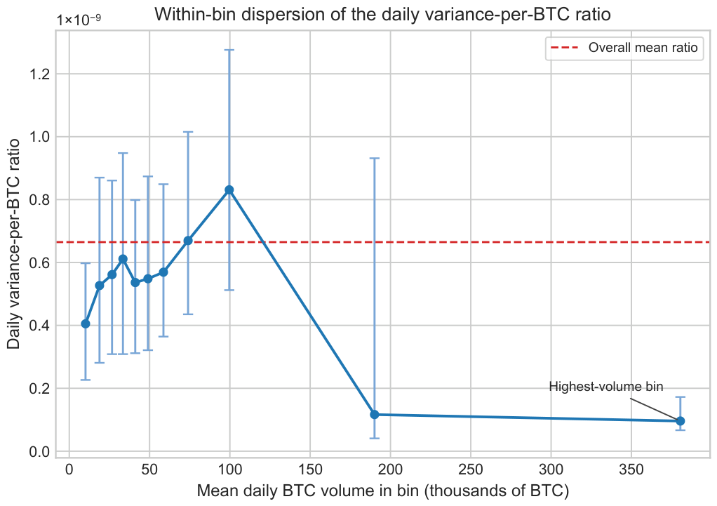
Figure A1 reports the within-bin dispersion of the daily variance-per-BTC ratio across the same volume bins used in the main paper’s scatter plot. The central bins cluster around the overall mean ratio, while the highest-volume bin is visibly attenuated. This is why the main text describes the variance–volume evidence as first-order compatibility rather than as a literal invariance result.
Figure A1.
Within-bin dispersion of the daily variance-per-BTC ratio across volume bins for BTC/USDT, Binance, 2020–2025. Points show the within-bin median ratio and bars show the interquartile range. The dashed line is the overall mean ratio. The main takeaway is that the central bins cluster around a fairly stable ratio, while the highest-volume bin shows clear attenuation.
Appendix C.2. Volume-Conditioned Variance-Matched Increment Benchmark
The main text’s Q–Q plot fixes only the horizon and the sample-average hourly volume. Here the analysis conditions more tightly on realized one-hour volume. This subsection still studies a variance-matched benchmark rather than the exact increment law of the general framework. For each hour t, define the standardized increment
where is the simple one-hour return, is the sample mean one-hour return, is the observable variance-per-BTC moment, and is realized one-hour BTC volume. Under the symmetric queueing benchmark, the corresponding conditional law is
Using the observed sequence over 48,374 hourly bars and 8 simulated draws per hour, the empirical standardized middle quantiles are
versus model-implied quantiles
The model-implied central 80% band therefore covers 85.3% of standardized observations, and the model-implied central 50% band covers 60.7%. The corresponding empirical/model width ratios are 0.862 for the 80% band and 0.756 for the 50% band. Ratios below one mean that the model-implied central bands are wider than the empirical center. Volume conditioning thus improves the middle-quantile comparison relative to the unconditional benchmark in the main text, but the symmetric variance-matched core still overstates central dispersion somewhat and does not eliminate tail misspecification.
Appendix C.3. Sub-Sample Reduced-Form Checks
The main paper now reports 2020–2022, 2023, and 2024–2025 side by side so the reader can see directly that the reduced-form liquidity and resiliency moments move across major market phases. This appendix keeps the earlier endpoint contrast only as a compact descriptive comparison between the pre-transition window and the later ETF-era window; 2023 is treated in the main paper as the transition year rather than excluded from the evidentiary record.
Interpretation
The earlier sub-sample windows show somewhat heavier trading intensity (3986 BTC versus 1305 BTC per one-hour bar), while the later window shows a larger variance-per-BTC estimate ( the 2020–2022 value) together with slower effective mean reversion ( versus ). Those comparisons are descriptive rather than structural. Once the symmetry mapping is re-imposed on short sub-samples, contingent quantities such as , , and can move substantially even when the directly observed moments change only moderately. For that reason, the main text keeps the structural translations at the full-sample level and uses the sub-sample checks only to show that the reduced-form diagnostics remain regime-dependent.
Appendix C.4. Addressing the Tail Risk Challenge
Appendix C.4.1. Scope
The Skellam (or NB–Skellam) core provides a useful baseline for normal trading periods and a coarse description of the center of the unconditional one-hour increment distribution. The far tails during stress periods necessarily require an additional component—such as a core–Normal/tail–Student-t mixture—to improve tail coverage relative to the Gaussian benchmark.
The one-hour return series has empirical excess kurtosis . By comparison, the count-space Poisson term is only and the count-space NB approximation rises only to . Rather than invalidating the baseline interpretation, this gap delineates the domain over which the core specification is useful:
What the Model Captures Well (the bulk of central observations):
- Normal market conditions with continuous order flow.
- Gradual order-flow shifts across descriptive market phases.
- Routine volatility from imbalanced arrival rates.
- Mean-reversion from latent occupancy unwinding.
What Requires Extensions (stress-period tail events):
- Exchange hacks or policy shocks.
- Coordinated whale movements.
- Cascading liquidations from leveraged positions.
- Technological disruptions (forks, 51% attacks).
Appendix C.4.2 shows that a two-component mixture improves unconditional tail coverage materially relative to a rolling Gaussian benchmark, but still falls short of exact 99% unconditional coverage and continues to show violation clustering during stress episodes. In that specification, the queueing-motivated core benchmark describes normal times while a heavy-tailed Student-t component captures crisis periods. The core model provides the baseline; practitioners must still add a stress-state layer for tail-risk work.
This parallels established practice in equity markets, where models capture normal volatility but require separate treatment of crashes (Bates, 2000). The paper’s narrower contribution is to characterize normal order-flow dynamics before turning to extreme events.
Appendix C.4.2. Heavy-Tail Regime Switch
Pure Skellam dynamics capture normal order-flow fluctuations but miss the extreme tails seen in realised returns. The hourly return is therefore modeled as a two-component mixture described in Appendix E. This subsection uses a 1 h VaR overlay based on a core-Normal/tail-Student-t mixture with threshold at , estimated by a threshold split rather than by full EM-MLE.
where the core component is fit on the in-threshold observations and is only queueing-motivated rather than queueing-imposed, while the stress component adds a near-zero-mean Student-t shock with scale and degrees of freedom .4
Parameter Estimation
Equation (A16) is fit descriptively to the 2020–2025 Binance hourly close-to-close returns. The full-sample parameter estimates are
For risk management, however, the paper evaluates this specification in a rolling out-of-sample backtest rather than relying on the full-sample fit alone. The intent is pragmatic tail augmentation, not structural identification from the queueing model.
Risk Metrics
The one-hour 99% Value-at-Risk is the 1% quantile of the mixture. In the rolling backtest used in the main text, the average one-hour forecast is
Back-Test
Using trailing 2160 h estimation windows and re-fitting every 24 h, the mixture produces VaR breaches over n = 46,214 out-of-sample hourly forecasts (1.13%). The Kupiec unconditional-coverage statistic is
yielding a p-value of 0.008. Relative to the rolling Gaussian benchmark (breach rate 1.80%), the mixture improves unconditional coverage materially. It nevertheless still misses exact 99% unconditional coverage at conventional levels, whereas rolling historical simulation (1.07%) is slightly closer to nominal unconditional coverage in this sample. The mixture is retained because it is a compact parametric monitoring overlay tied to the same one-hour variance normalization as the core benchmark, not because it dominates nonparametric forecasting. Violation clustering remains visible in stress episodes even after the unconditional fit improves.
Interpretation
Only 4.8% of the time does the market enter the stress state, but in that regime the scale of shocks () is roughly five times the core Skellam standard deviation (), contributing substantially to the empirical excess kurtosis of reported in the main paper’s empirical summary table.
This appendix evidence sharpens the paper’s risk interpretation by the following:
- Separating the descriptive full-sample fit from the rolling out-of-sample evaluation;
- Showing that the stress-state layer improves on a Gaussian benchmark for unconditional 99% coverage without fully solving it;
- Quantifying how much additional tail thickness is needed beyond the queueing core.
Appendix C.5. Parameter Evolution and Stability
The main paper reports rolling estimates of the feedback proxy and the effective mean-reversion rate across 30-day windows. The informative empirical result is the variation in those directly monitored quantities: the full-sample proxy is positive, while rolling mean reversion weakens materially and sometimes turns negative. Any accompanying symmetry-based quantities remain secondary descriptive translations rather than additional sources of identification.
Appendix C.6. Rolling-Window-Length Sensitivity
Because the 30-day rolling share of windows with is a visible headline number in the main paper, Table A3 checks the same descriptive statistic under shorter and longer overlapping windows and under more conservative sampling schemes for the 30-day window. The point of that table is modest: it does not create new identification, but it shows that the point-sign summary is not unique to a single exact window length or a single exact overlap convention. Table A4 then adds the uncertainty-aware 30-day classification used in the main text. The baseline classification uses a one-standard-error buffer in the lag-1 autocorrelation, , which corresponds to the near-zero region around zero in the autocorrelation scale. This is a heuristic monitoring rule rather than a formal confidence interval under heteroskedastic, serially dependent returns. As a more conservative companion heuristic, doubling the buffer to leaves 17.2% of overlapping windows clear positive, 79.9% ambiguous, and 2.9% non-positive. The main qualitative message is unchanged: ambiguity dominates once one moves away from the raw point-sign share.
Table A3.
Sensitivity of the rolling sign summary for to window length. The shares remain descriptive because the windows overlap heavily.
Table A4.
Heuristic uncertainty-aware classification for the 30-day rolling summary. “Clear positive” means the implied lag-1 autocorrelation is below , “non-positive” means it is above , and the middle region is classified as ambiguous. The rule is a monitoring buffer, not a formal dependence-robust interval.
In the day-ahead monitoring exercise reported in the main paper, this doubled companion buffer leaves 347 clear-positive predictor days and 59 non-positive predictor days, with corresponding next-day tail-day rates of 6.9% and 15.3%, respectively. The doubled-buffer comparison is therefore kept only as a directional companion check rather than as a primary classification result.
Appendix C.7. Post-Shock Recovery by Rolling Resiliency Regime
The main paper interprets only as a local descriptive recovery-timescale diagnostic. To connect that language to realized paths, this appendix reports one narrow event study using the existing hourly returns and the existing rolling 30-day regime labels. Isolated large shocks are identified as the top 97.5% of absolute one-hour returns among hours with valid 30-day classifications, with only local maxima within ±6 h retained and candidate shocks de-overlapped within the following 24 h. This leaves 497 events. For an event at hour t with return and sign , define the aligned remaining displacement after h hours as
By construction, . Lower values indicate more reversal of the initial shock, and corresponds to a full reversal by horizon h.
Table A5 and Figure A2 show a clear ordering for these rare isolated shocks. Mean initial shock magnitudes are similar across regimes (about 3% of price), but the subsequent paths differ. After 6 h, the mean aligned remaining displacement is 0.907 in clear-positive windows, versus 0.946 in non-positive windows and 1.025 in ambiguous windows. After 24 h, the same ordering remains: 0.795 in clear-positive windows, 0.890 in non-positive windows, and 1.017 in ambiguous windows. The corresponding mean 24 h reversal shares are 20.5%, 11.0%, and %. This is still only a threshold-specific descriptive check, but it gives a direct path-based complement to the next-day sorting exercise in the main text: the rolling resiliency classification is associated not only with next-day risk levels, but also with visibly different recovery paths after large isolated shocks.
Table A5.
Post-shock recovery by rolling 30-day resiliency regime for isolated large hourly shocks on Binance BTC/USDT, 2020–2025. Shocks are the top 97.5% of absolute one-hour returns among hours with valid rolling classifications, restricted to local maxima within ±6 h and de-overlapped within the following 24 h. Lower remaining displacement indicates faster reversal of the initial shock.
Figure A2.
Aligned post-shock recovery paths by rolling 30-day resiliency regime for isolated large hourly shocks on Binance BTC/USDT, 2020–2025. Event hours are the top 97.5% of absolute hourly returns among observations with valid rolling classifications, restricted to local maxima within ±6 h and de-overlapped within the next 24 h. The vertical axis reports aligned remaining displacement, normalized so the shock hour starts at 1; lower paths indicate faster reversal, and the dotted zero line corresponds to full reversal of the initial shock. Clear-positive windows recover more over the next 24 h than ambiguous or non-positive windows in this narrow descriptive check; event counts by regime appear in Table A5.
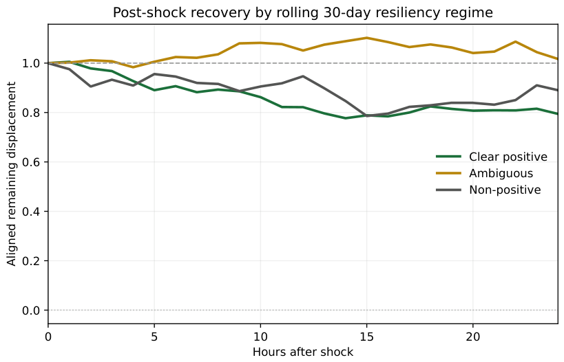
Appendix C.8. Comparison with Standard Trade-Based Liquidity Benchmarks
To see whether the rolling liquidity monitor is just a renamed version of standard trade-based measures, this subsection compares rolling with two benchmarks that can be constructed from the same public Binance trade-print data. Both benchmarks are constructed from the identical public Binance trade-print panel used for the main diagnostics. The first is a rolling 30-day Amihud illiquidity proxy, defined as the 30-day mean of daily , where is the UTC-day close-to-close return and is daily dollar volume. The second is a rolling 30-day median of the absolute daily minute signed-flow slope from the day-by-day directional-impact regressions, used here as a trade-print-feasible Kyle-style minute signed-flow impact benchmark. The benchmark comparison follows the same 30-day day-ahead design as the monitoring exercise reported in the main paper, but it begins one day later because the rolling Amihud series needs 30 non-missing daily return-volume observations. The resulting matched benchmark sample contains 1986 predictor days from 31 January 2020 through 8 July 2025, with 15 matched days containing fewer than 24 hourly returns because of the observed missing UTC hours.
Table A6 shows two things. First, rolling is related to these familiar trade-based measures but not identical to them: its correlation is 0.304 with rolling Amihud illiquidity and 0.630 with the Kyle-style minute signed-flow impact benchmark. Second, rolling sorts next-day stress more sharply in this matched benchmark sample. The high-minus-low next-day tail-day spread is 8.6 percentage points for rolling , compared with 4.7 for rolling Amihud and 1.1 for the Kyle-style minute-impact benchmark. The corresponding high/low next-day realized-variance ratios are 2.76, 1.68, and 1.04. This still falls short of a formal forecast horse race, but it addresses the narrow benchmark question directly: the queueing-organized liquidity monitor is positively related to feasible standard trade-based measures while not being redundant with either of them in the same day-ahead design.
Order-book depth measures are not added in this comparison because the public Binance data used here contain trade prints and aggressor-side information, not synchronized order-book snapshots. A depth comparison would require a different data source and a different reconstruction pipeline.
Table A6.
Matched benchmark-sample comparison of rolling with standard trade-based liquidity benchmarks. All predictors are measured at the end of UTC day d using trailing 30-day windows and are compared with the realized outcomes on day . Correlations with rolling are reported in the text; the table concentrates on the day-ahead stress-sorting comparisons.
Appendix C.9. Nearby-Frequency Robustness of the Feedback Splice
The headline proxy combines a directional-impact scale from signed-flow regressions with a lagged signed-BTC-flow slope. Because those ingredients are estimated at different frequencies, two nearby alternatives are reported here. The first replaces the baseline 1 min directional scale with a 5 min directional scale computed by the same day-by-day procedure on 5 min buckets. The second replaces the baseline 1 h flow regression with a non-overlapping 2 h block regression and rescales the resulting cumulative signed-flow slope back to a per-hour feedback coefficient.
Table A7.
Nearby-frequency robustness for the proxy feedback coefficient. All three full-sample variants remain positive and stay within the same order of magnitude as the baseline estimate.
The 5 min directional alternative is 0.914 times the baseline value, while the 2 h flow alternative is 0.576 times the baseline. These checks do not transform the splice into a directly identified structural estimate, but they do show that the positive sign and rough magnitude of the proxy are not tied to a single exact pair of sampling choices.
Appendix C.10. Secondary ρ Summary
The ratio
remains available as a compact symmetry-based summary. In the full sample, the contingent structural translation gives and . Those quantities are kept in the appendix rather than the main text because they do not add independent identifying information beyond the directly monitored pair . Near the regime boundary, small movements in can make move sharply, which is why the main paper treats it as secondary.
Appendix C.11. Risk Management Performance
This appendix backtests rolling one-hour 99% VaR forecasts rather than a fixed in-sample threshold. The pure queueing/Gaussian benchmark implies an average VaR of 1.51% and yields a breach rate of 1.80%, materially above the 1% target. The stress-state mixture raises the average forecast to 1.84% and lowers the breach rate to 1.13%, while rolling historical simulation gives 1.87% and 1.07%. The main text therefore uses the mixture only as a pragmatic parametric tail overlay: it improves materially on the Gaussian benchmark, but its Kupiec p-value of 0.008 still rejects exact unconditional 99% coverage. Historical simulation remains slightly closer to nominal unconditional coverage in this sample.
Appendix C.12. Robustness Tests
The appendix robustness notes are kept short because the main paper already reports the core reduced-form evidence. Two points matter most. First, the rolling estimates reported in the main paper show local variation rather than a single stable resiliency regime: a non-trivial minority of windows have and are better interpreted as local momentum or stress windows than as mean-reverting calibrations. Second, the auxiliary robustness material here is meant only to show that reasonable specification changes leave the paper’s descriptive hierarchy intact: the main evidence remains the observable liquidity, signed-flow, and resiliency diagnostics reported in the main text.
Exchange-specific data requirement: The present implementation relies on Binance trade-print files together with aggressor-side information recoverable from the Binance schema (including isBuyerMaker). Extending the workflow to other venues would require rebuilding venue-specific trade-print and aggressor-side panels, so multi-venue replication is left to future work rather than asserted as cross-venue equivalence here.
Appendix C.13. Limitations and Future Data Work
A dedicated cross-venue robustness study would require harmonised fill-level data and aggressor-side reconstruction across heterogeneous APIs. That exercise is therefore left to future work.
Appendix D. Coverage and Reconciliation of Public OHLCV Feeds
Public OHLCV aggregates (e.g., Binance “klines” and widely mirrored third-party files) do not provide the trade-print and aggressor-side fields required for the present calibration. The narrower point is that the present manuscript calibrates on full trade-print data rather than on public OHLCV aggregates, because the queueing, signed-flow, and aggressor-side diagnostics require fields that OHLCV files do not retain.
Appendix E. Estimation Details for the Core/Stress Mixture
The estimator uses a threshold split rather than full EM-MLE. The threshold is , and the mixture weights are and . The estimation procedure is as follows:
- Compute the empirical hourly return standard deviation ; set the stress threshold .
- Core sample → fit via maximum-likelihood estimation.
- Tail sample → fit Student-, same optimisation call.
- Mixture weights .
- 99% one-period VaR is .
- Back-test: 520 breaches out of 46,214 one-hour forecasts ⇒ unconditional coverage 1.13%.
The identical numerical values are reported in Appendix C.4.2 (, ).
Appendix F. Monte Carlo Validation of the Variance-Scale Estimator
The Monte Carlo experiment simulates 1000 independent paths with illustrative parameters , h and (chosen for computational tractability; the bias test is scale-invariant). In each path, the variance-scale coefficient is estimated from the same sample ratio used in the main paper’s empirical-implementation subsection. Table A8 summarizes bias and dispersion.
Table A8.
Finite-sample performance of the variance-scale estimator (1000 replications).
Bias is statistically indistinguishable from zero and the RMSE follows the benchmark, confirming practical unbiasedness for sample windows of a few weeks or longer (see Figure A3).
Figure A3.
Finite-sample precision of the variance-scale estimator. Natural-log plot of sample length T (hours) versus the standard deviation of obtained from 1000 Monte Carlo replications (blue dots). The red line is the OLS fit: , , confirming the expected rate.
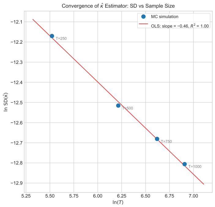
Appendix G. Occupancy of a Discrete-Time GI/Geo/∞ Queue
Let be the time tick. In tick the numbers of new long- and short-side latent occupancy units are independent
An existing long-side occupancy unit survives to the next tick with probability ; a short-side occupancy unit survives with .
Let and denote the outstanding long- and short-side occupancies at the start of tick n and define .
Proposition A1.
In steady state
Moreover, and are independent. Consequently, .
Proof.
Consider the long-side queue; the short-side queue follows identically. Given , the number of long-side occupancy units that survive to the next tick is . Thus
With , independence of gives the recursion . A stationary solution must satisfy . The unique pgf with is provided , establishing the Poisson law.
Independence of and follows from independent arrivals and services together with the PASTA property of Poisson processes (Wolff, 1982). The Skellam result is the difference of two independent Poisson variates. □
Appendix H. Piecewise Linear Depth and Price Moments
Partition the inventory space into three symmetric regions
and define the impact schedule
Let and define .
Proposition A2.
The first two unconditional moments of are
Each truncated sum involves a finite number of Skellam probabilities
Proof.
Derivation of the Count-Space Burstiness Approximation
The main text’s count-space burstiness formula is an approximation for the excess kurtosis of the hourly increment . This subsection first records the exact common-rate Gamma–Poisson cumulant ratio and then shows the simpler proxy reported in the main text.
Let
where the buy and sell counts may have different shape parameters but share a common Gamma rate , matching the main text’s Negative-Binomial parameterization . Write , so . Under this single shape–rate parameterization, the cumulant generating function of is
For the difference ,
Because odd cumulants change sign under while even cumulants do not, the second and fourth cumulants of are just the sums of the side-specific even cumulants:
Writing , the exact common-rate excess kurtosis becomes
The main text uses the simpler proxy
which preserves the familiar Poisson benchmark term plus the over-dispersion term . The approximation is therefore not an exact common-rate identity; it replaces the smaller exact remainder by the Poisson benchmark to keep the decomposition transparent. In the paper, this is used only as a burstiness proxy for hourly buy/sell trade counts. It is not presented as a fully general return-law derivation.
Appendix I. NB–Skellam Distribution
When long- and short-side occupancy counts follow Negative-Binomial distributions (arising from Gamma-mixed Poisson processes), their difference follows a NB–Skellam distribution.
Note on empirical relevance. With the empirical dispersion parameters and (Gamma–Poisson mixing), the NB–Skellam does not collapse to the standard Skellam. The arrival-rate coefficients of variation are and , and the corresponding burstiness proxy contributes about to the excess-kurtosis decomposition under the approximation above, both materially different from the Poisson–Skellam benchmark. In the Binance data, however, NB–Skellam still understates the extreme tails in hourly returns, which is why this count-space extension is retained only as a supplementary burstiness note alongside the separate stress overlay.
Notes
| 1 | The modified Bessel function of the first kind arises naturally in circular statistics and here characterizes the difference of Poisson variates. |
| 2 | “Non-missing” means windows for which the rolling return autocorrelation and signed-flow regression are both computable once the observed missing UTC hours are carried through the hourly grid. The count therefore differs slightly from the purely mechanical number of overlapping 30-day calendar windows. The sample contains 34 missing UTC hours overall, so a small number of windows lose one or more hourly observations even though the rolling clock continues to advance. |
| 3 | s keeps the Poisson means in the low teens, striking a good balance between numerical accuracy and computational speed. If finer granularity is desired, set s; all formulas below continue to apply after replacing accordingly. |
| 4 | Because the empirically estimated Negative-Binomial shape parameters are small (, ), their contribution to excess kurtosis is small relative to the stress-state Student-t term. Hence the queueing variance is best read here as motivation and comparison for , not as a hard estimation constraint. |
References
- Alexander, C., Deng, J., Feng, J., & Wan, H. (2023). Net buying pressure and the information in bitcoin option trades. Journal of Financial Markets, 63, 100764. [Google Scholar] [CrossRef] [Scilit]
- Amihud, Y., & Mendelson, H. (1980). Dealership market: Market-making with inventory. Journal of Financial Economics, 8(1), 31–53. [Google Scholar] [CrossRef] [Scilit]
- Anastasopoulos, A., Gradojevic, N., Liu, F., Maynard, A., & Tsiakas, I. (2026). Order flow and cryptocurrency returns. Journal of Financial Markets, 101047, Advance online publication. [Google Scholar] [CrossRef] [Scilit]
- Bates, D. S. (2000). Post-’87 crash fears in the s&p 500 futures option market. Journal of Econometrics, 94, 181–238. [Google Scholar] [CrossRef] [Scilit]
- Binance. (2025). Historical spot market data: Btcusdt daily trades. Available online: https://data.binance.vision/?prefix=data/spot/daily/trades/BTCUSDT/ (accessed on 28 July 2025).
- Bouchaud, J.-P., Farmer, J. D., & Lillo, F. (2009). How markets slowly digest changes in supply and demand. In T. Hens, & K. R. Schenk-Hoppe (Eds.), Handbook of financial markets: Dynamics and evolution (pp. 57–160). Elsevier. [Google Scholar] [CrossRef] [Scilit]
- Cont, R., & de Larrard, A. (2013). Price dynamics in a markovian limit order market. SIAM Journal on Financial Mathematics, 4(1), 1–25. [Google Scholar] [CrossRef] [Scilit]
- Dimpfl, T. (2017). Bitcoin market microstructure. SSRN Electronic Journal. [Google Scholar] [CrossRef] [Scilit]
- Foucault, T., Pagano, M., & Röell, A. (2013). Market liquidity: Theory, evidence, and policy. Oxford University Press. [Google Scholar] [CrossRef] [Scilit]
- Garriott, C., van Kervel, V., & Zoican, M. (2025). Queuing and inventories in limit order markets. Journal of Financial Markets, 75, 100982. [Google Scholar] [CrossRef] [Scilit]
- Ho, T., & Stoll, H. R. (1981). Optimal dealer pricing under transactions and return uncertainty. Journal of Financial Economics, 9(1), 47–73. [Google Scholar] [CrossRef] [Scilit]
- Kim, S. T., & Stoll, H. R. (2014). Are trading imbalances indicative of private information? Journal of Financial Markets, 20, 151–174. [Google Scholar] [CrossRef] [Scilit]
- Koopman, S. J., Lit, R., & Lucas, A. (2017). Intraday stochastic volatility in discrete price changes: The dynamic skellam model. Journal of the American Statistical Association, 112(520), 1490–1503. [Google Scholar] [CrossRef] [Scilit]
- Kyle, A. S. (1985). Continuous auctions and insider trading. Econometrica, 53(6), 1315–1336. [Google Scholar] [CrossRef] [Scilit]
- Palm, C. (1943). Intensitätsschwankungen im fernsprechverkehr. Ericsson Technics, 44, 1–189. [Google Scholar]
- Stoll, H. R. (1978). The supply of dealer services in securities markets. Journal of Finance, 33(4), 1133–1151. [Google Scholar] [CrossRef]
- Wolff, R. W. (1982). Poisson arrivals see time averages. Operations Research, 30, 223–231. [Google Scholar] [CrossRef] [Scilit]
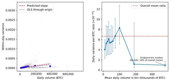
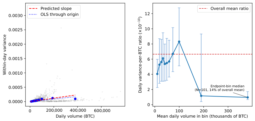
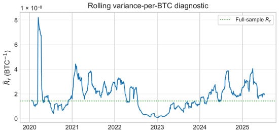
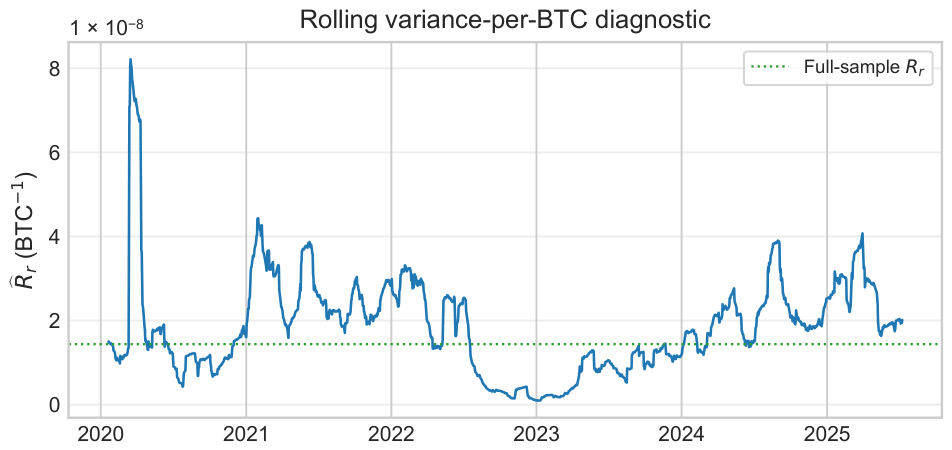
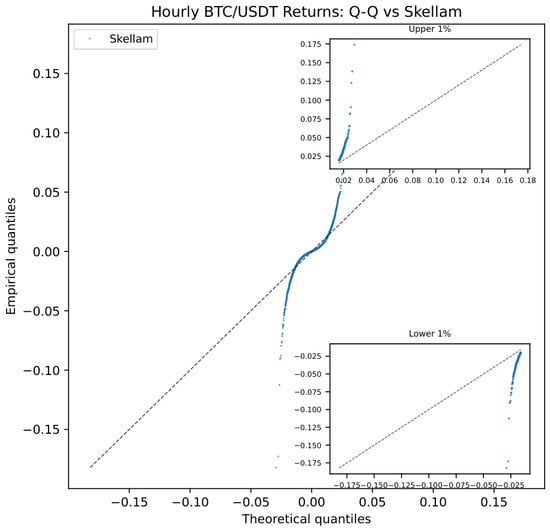
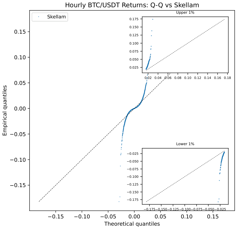
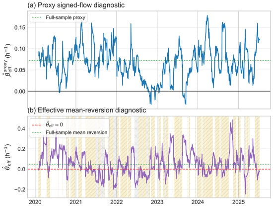
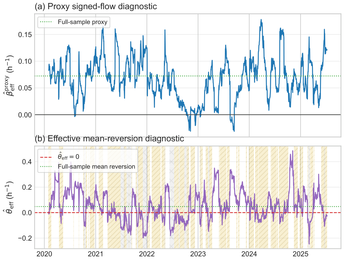

Disclaimer/Publisher’s Note: The statements, opinions and data contained in all publications are solely those of the individual author(s) and contributor(s) and not of MDPI and/or the editor(s). MDPI and/or the editor(s) disclaim responsibility for any injury to people or property resulting from any ideas, methods, instructions or products referred to in the content. |
© 2026 by the author. Licensee MDPI, Basel, Switzerland. This article is an open access article distributed under the terms and conditions of the Creative Commons Attribution (CC BY) license.