Carbon Exposure and Corporate Cash Holdings: International Evidence from the Paris Agreement

Abstract

We ask whether an increase in the salience of climate-transition risk changes corporate liquidity policy. Using the December 2015 Paris Agreement as a global shock, we estimate a difference-in-differences model using 1745 listed non-financial firms from 55 countries over 2010–2025. Firms in the top quartile of pre-treatment carbon intensity (CO₂ emissions scaled by revenue in 2015) are classified as treated. In our preferred specification, which includes firm fixed effects and industry-by-year fixed effects with standard errors two-way clustered by firm and year, the cash-to-net-assets ratio of treated firms rises by 2.17 percentage points relative to less carbon-intensive peers after 2015. This effect is equivalent to approximately 14.9% of the full-sample mean and is statistically significant at the 10% level. In the event study, the five pre-treatment coefficients for 2010–2014 are small and individually insignificant, but their joint test rejects the null under two-way clustering, so the evidence on parallel pre-trends is sensitive to the inference procedure; the post-treatment coefficients turn positive around 2019 and remain positive through 2025. In a 500-replication randomisation-inference placebo test, the actual estimate lies toward the upper tail of the placebo distribution (empirical two-sided p = 0.0978). The coefficient remains positive under propensity-score matching, country-by-year fixed effects, alternative sample windows, an alternative scaling of the cash variable, a 50th-percentile treatment cut-off, and the exclusion of potential post-treatment controls, although several of these estimates are only marginally significant. The level of cash does not increase, so the result concerns the cash ratio rather than cash accumulation. Exploratory analysis using the Whited–Wu index is consistent with, but does not establish, a financing-constraints channel. Because the design cannot separate the Agreement itself from subsequent implementation and other post-2015 developments, we interpret the result as an association between the post-Paris transition-policy environment and a relative rise in the cash ratios of carbon-intensive firms, which we regard as suggestive rather than conclusive evidence of a precautionary response to climate-policy uncertainty.

1. Introduction

Climate change reaches corporate balance sheets through two distinct channels. Physical risk operates through the direct damage that a changing climate inflicts on assets, supply chains, and markets. Transition risk operates through the policy, technological, and preference shifts that accompany decarbonisation, and it bites hardest for firms whose production processes are carbon-intensive. Because transition risk is fundamentally a policy risk, it is unusually sensitive to discrete political events. The Paris Agreement, adopted on 12 December 2015 and signed by 195 parties, is the single most visible event of this kind in the past two decades; for the first time, essentially every major economy committed to a long-run decarbonisation trajectory, and carbon-intensive business models acquired an explicit, internationally coordinated expiry horizon.

A substantial body of literature now documents that capital markets have priced this risk. Carbon-intensive firms earn a return premium (Bolton & Kacperczyk, 2021, 2023), carry fatter left tails in their option-implied return distributions (Ilhan et al., 2021), pay more for bank credit (Delis et al., 2024; Javadi & Masum, 2021), and attract closer scrutiny from institutional investors concerned with regulatory exposure (Krueger et al., 2020). What remains less well understood is how managers respond. If the cost and availability of external finance deteriorate for carbon-intensive firms, and if the timing and severity of future climate regulations are themselves uncertain, then the classic precautionary motive for holding cash (Opler et al., 1999; Bates et al., 2009; Han & Qiu, 2007) predicts that these firms should build liquidity buffers. Cash is the most flexible response available to a firm facing a risk whose arrival date is unknown: it can be accumulated quietly; held indefinitely; and deployed against compliance costs, abatement investment, or refinancing gaps as they materialise.

This paper tests that prediction. We assemble an international panel of 1745 listed non-financial firms from 55 countries with pre-Paris carbon-emissions information and non-missing carbon intensity in 2015, and we estimate a difference-in-differences (DiD) specification in which treatment status is determined by a firm’s carbon intensity in 2015, the last full year before the Agreement. Firms in the top quartile of the 2015 distribution of CO₂ emissions per unit of revenue are treated; the remainder form the control group. Because treatment status is fixed at a pre-event value and the shock is a single global event date, the design avoids the negative-weighting problems that afflict staggered adoption settings, and it allows firm and year fixed effects to absorb time-invariant heterogeneity and common macroeconomic shocks.

Three findings emerge. First, in our preferred specification with firm fixed effects, industry-by-year fixed effects, and standard errors two-way clustered by firm and year, the cash-to-net-assets ratio of carbon-intensive firms rises by 2.17 percentage points relative to their peers after 2015. The estimate is statistically significant at the 10% level and corresponds to approximately 14.9% of the full-sample mean. Second, the timing is informative. An event-study specification shows five pre-treatment coefficients for 2010–2014 that are small and individually insignificant. Their joint test does not reject the null under robust or firm-clustered standard errors, but it does under two-way clustering, so the evidence on parallel pre-trends is sensitive to the inference procedure and should be read with caution. The post-treatment coefficients remain flat through 2018, turn positive from 2019 onward, peak in 2022, and remain significantly positive through 2025. The delayed response is consistent with a slow-moving adjustment to a policy signal whose concrete national implementation—including carbon pricing schemes, disclosure mandates, and sectoral phase-out timetables—arrived only gradually after 2016, although the design cannot separate the Agreement itself from this later implementation or from other contemporaneous developments. Third, the coefficient remains positive across the reported checks: the actual estimate lies toward the upper tail of the 500 placebo estimates (empirical two-sided p = 0.0978), and the coefficient stays positive under propensity-score matching, country × year fixed effects, the exclusion of COVID-19 years, a shortened sample window, an alternative cash measure, a 50th-percentile treatment cut-off, and the exclusion of potential post-treatment controls, although several of these estimates are only marginally significant. Because the logarithm of cash does not increase, the evidence concerns a relative rise in the cash ratio rather than an accumulation of cash.

We then explore a financing-friction channel. A bootstrapped mediation test using the Whited and Wu (2006) financial constraints index yields a positive indirect effect. Because the index is a composite proxy rather than a direct observation of credit conditions, and because the proportion mediated is imprecisely estimated, we treat this analysis as exploratory evidence that is consistent with, but does not establish, a financing-constraints channel (Section 5.2).

The paper is closely related to recent studies linking climate risk to corporate cash holdings. Wu et al. (2025) showed that high-carbon emitters increased their cash holdings relative to low-carbon emitters after the Paris Agreement and attributed this response to a precautionary motive; Tran et al. (2025) examined carbon emissions, firm-level climate change exposure, and cash reserves in 51 countries and used the Paris Agreement in a difference-in-differences robustness design; and Wang et al. (2026) used the Agreement as an exogenous shock to study how perceived climate risk affects cash holdings. We therefore do not claim originality for the link between climate risk and cash holdings, for the post-Paris rise in cash among carbon-intensive firms, or for cross-country evidence as such. Our contribution is narrower and mainly concerns the design. First, treatment is assigned from a single pre-event cross-section of carbon intensity measured in 2015, and entry into the sample does not depend on post-event disclosure, so the estimates do not condition on a post-treatment variable. Second, the preferred specification absorbs industry-by-year shocks, so the estimate compares firms in the same industry and year that differ in pre-event carbon intensity rather than emission-intensive and asset-light industries. Third, we trace the full dynamic path through 2025 under clustered inference, with a joint pre-trend test and randomisation inference that preserves the actual treated share; the relative rise in cash ratios emerges only from 2019 and persists for several years. Fourth, we examine whether measured financing constraints move with cash holdings while treating this analysis as exploratory. More broadly, the findings complement evidence that carbon-risk exposure is associated with lower leverage (Nguyen & Phan, 2020) by documenting a parallel adjustment in the cash ratio.

The remainder of the paper is organised as follows. Section 2 develops the hypotheses. Section 3 describes the data, variables, and identification strategy. Section 4 presents the results. Section 5 discusses the findings and their limitations and implications. Section 6 concludes the paper.

2. Literature Review and Hypothesis Development

2.1. Carbon Risk and the Cost of Capital

Transition risk enters firm value through expected cash flows and discount rates. On the cash-flow side, carbon-intensive firms face the prospect of explicit carbon prices, tightening emissions caps, compulsory abatement investment and, in the limit, the stranding of long-lived assets. On the discount-rate side, investors who anticipate these outcomes require compensation for bearing them. Bolton and Kacperczyk (2021) showed that US firms with higher emissions levels and higher emissions growth earn higher returns, a premium they attributed to transition-risk compensation rather than to unpriced ESG preferences, and Bolton and Kacperczyk (2023) extended the result to a cross-section of 77 countries. Ilhan et al. (2021) documented that the cost of protecting against downside tail risk is markedly higher for carbon-intensive firms, and that this wedge widens after events that raise climate-policy salience.

Credit markets respond similarly. Javadi and Masum (2021) found that firms exposed to greater climate risk pay higher spreads on bank loans, and Delis et al. (2024) showed that lenders began pricing fossil-fuel reserves as a stranded-asset risk after the Paris Agreement specifically. Seltzer et al. (2022) reported that bonds of firms with poor environmental profiles carry lower credit ratings and higher yields, with effects concentrated in states with stricter regulation. Taken together, this evidence establishes that after 2015, carbon-intensive firms faced a costlier and less certain external financing environment.

2.2. Precautionary Savings and Policy Uncertainty

The precautionary motive is the dominant explanation for the secular rise in corporate cash. Opler et al. (1999) showed that firms with riskier cash flows and poorer access to capital markets hold more cash. Almeida et al. (2004) formalised the idea that financially constrained firms systematically save out of cash flow in order to preserve future investment capacity, whereas unconstrained firms do not. Han and Qiu (2007) demonstrated that cash-flow volatility raises cash holdings precisely for constrained firms, and Bates et al. (2009) attributed the doubling of US cash ratios between 1980 and 2006 largely to rising idiosyncratic risk. Denis and Sibilkov (2010) showed that the marginal value of a dollar of cash is higher for constrained firms, confirming that these buffers are value-relevant rather than a symptom of agency problems.

Policy uncertainty is a natural source of the risk that drives this motive. Phan et al. (2019) and Duong et al. (2020) both found that US firms increase cash holdings when economic policy uncertainty rises, and that the effect is strongest among financially constrained firms and those with limited access to external capital. Climate policy is a particularly acute instance of this general phenomenon. Unlike a monetary or fiscal shock, the transition is a multi-decade process whose intermediate path—the timing of carbon prices, the stringency of sectoral mandates, and the speed of technological substitution—is deeply uncertain, even though its direction is not. For a carbon-intensive firm, the Paris Agreement did not resolve uncertainty; it announced that a costly adjustment was coming without specifying when, how much, or through which instrument. This is the configuration under which precautionary saving is most valuable.

This reasoning yields our primary hypothesis.

H1. 

Following the Paris Agreement, firms with high pre-treatment carbon intensity increase their cash holdings relative to firms with low carbon intensity.

2.3. The Financing-Constraints Channel

If the mechanism is precautionary, the effect should operate through the financing environment that the firm faces. Two readings are possible, and they generate opposite signs, which is why the channel deserves explicit testing rather than assertion. Under a tightening reading, carbon-intensive firms find external finance scarcer and dearer after 2015, measured constraints rise, and cash is accumulated as a substitute for impaired market access. Under an adjustment reading, carbon-intensive firms respond to the transition signal by deleveraging and by shifting their asset mix toward liquidity, so that composite constraint indices—most of which load heavily on leverage, size, and payouts—fall mechanically as the firm becomes more conservatively financed, with cash accumulation and measured constraint relief being two expressions of the same underlying balance-sheet adjustment.

Because the two readings cannot be distinguished by sign alone, we state the channel hypothesis in a neutral form and return to its interpretation in Section 5.

H2 (exploratory).

Following the Paris Agreement, the relative change in the cash holdings of carbon-intensive firms is accompanied by changes in measured financing constraints.

Bartram et al. (2022) provided the closest antecedent, showing that carbon-constrained US firms reallocate real activity and that financial constraints govern the size of that reallocation. Nguyen and Phan (2020) showed that carbon-risk exposure reduces leverage, whereas Ginglinger and Moreau (2023) documented a similar response to forward-looking physical climate risk, which is distinct from the transition risk studied here. Our analysis complements this evidence by examining the cash ratios of carbon-intensive firms; Section 1 sets out how our design relates to recent studies of climate risk and cash holdings.

3. Data and Methodology

3.1. Sample Construction

Firm-level financial and carbon intensity data were obtained from LSEG Workspace (London Stock Exchange Group plc, London, UK), while the macroeconomic variables (real GDP growth and CPI inflation) were obtained from the World Bank World Development Indicators. Carbon intensity is obtained directly from LSEG Workspace, and is defined as the sum of Scope 1 and Scope 2 CO₂ emissions scaled by total revenue. The underlying emissions data include both firm-disclosed values and values estimated by LSEG. We begin with an international panel of listed non-financial firms with firm-level environmental disclosure. The raw sample covers 10,510 firms and 85,866 firm-year observations over 2010–2025 after deleting observations before 2010 and the incomplete 2026 fiscal year. Requiring firms to report carbon emissions in at least one year before 2016 reduces the sample to 1930 firms and 28,481 firm-year observations. We then require non-missing carbon intensity data in 2015, the year used to determine treatment status, resulting in 1749 firms and 25,791 firm-year observations. Finally, after requiring non-missing values for all model variables, the estimation sample comprises 25,624 firm-year observations for 1745 firms from 55 countries. All firm-level continuous variables are winsorised at the 1st and 99th percentiles of the pooled 2010–2025 sample after the financial ratios are constructed. Appendix A (Table A1) presents the industry composition of the treated and control firms, providing additional evidence on the sectoral distribution of the two groups.

The sample requirement is restrictive by construction and introduces a survivorship dimension; firms that began disclosing emissions only after the Agreement, or that did not report a 2015 carbon intensity, are excluded. Firms are not required to report emissions after 2015, so continued post-event disclosure does not determine sample entry. We regard this as the correct trade-off. Assigning treatment from post-event emissions would contaminate the design, since the emission intensity observed after 2015 is itself an outcome of the treatment. Appendix B (Table A2) compares the pre-2016 characteristics of included and excluded firms. Included firms are significantly larger than excluded firms (difference = 0.412, t = 3.80, p < 0.001), while no statistically significant differences are observed in leverage, cash holdings, profitability, or book-to-market ratios. Section 5 discusses the external-validity consequences.

Table 1 defines the variables, Table 2 summarises the sample selection and attrition process, and Table 3 reports the geographic composition of the estimation sample.

Table 1. Variable definitions.

Variable	Definition
Dependent variables
CASHNO	Cash and cash equivalents divided by net assets (total assets − cash and cash equivalents). Primary dependent variable.
CASHAS	Cash and cash equivalents divided by total assets. Alternative dependent variable.
Independent variables
DID	TREATED × POST. Coefficient of interest.
TREATED	Indicator equal to one if a firm’s 2015 CO2 emission intensity, measured as total CO2 emissions scaled by total revenue, is at or above the 75th percentile of the 2015 cross-sectional distribution, and zero otherwise.
POST	Indicator equal to one for fiscal years 2016 onward, and zero otherwise.
Mediating variables
WW	Whited and Wu (2006) financial constraints index: WW = −0.091(CF/TA) − 0.062(DIVPOS) + 0.021(LTD/TA) − 0.044Ln(TA) + 0.102(ISG) − 0.035(SG) where CF/TA is cash flow divided by total assets; DIVPOS is a dummy variable equal to 1 if the firm pays dividends and 0 if otherwise; LTD/TA is long-term debt divided by total assets; Ln(TA) is the natural logarithm of total assets; ISG is industry sales growth; and SG is firm sales growth. Higher WW values indicate more severe financial constraints.
Control variables
AGE	Natural logarithm of firm age in years.
ROE	Net income divided by total equity.
GRO	Revenue growth, (Revenuet − Revenuet−1)/Revenuet−1.
BOARDSIZE	Natural logarithm of the number of board members.
LEV	Total liabilities divided by total assets.
CAPEXTA	Capital expenditures scaled by total assets.
BM	Book value of equity divided by market value of equity.
GDP	Annual real gross domestic product (GDP) growth rate of the country of headquarters.
CPI	Annual change in the Consumer Price Index of the country of headquarters.

Notes: All firm-level continuous variables are winsorised at the 1st and 99th percentiles. Country-level macroeconomic controls are matched to the firm’s country of headquarters.

Table 2. Sample selection and attrition.

Sample Selection Step	Firms	Observations
Initial sample of carbon-disclosing firms	10,510	85,866
Firms with carbon data before 2016	1930	28,481
Firms with carbon intensity data in 2015	1749	25,791
Final estimation sample with complete data for all model variables	1745	25,624

Table 3. Sample composition by region.

Region	Firms	Firm-Years	% of Firm-Years	Countries
Africa	61	891	3.48	3
Americas	481	6904	26.94	8
Asia	557	8340	32.55	19
Europe	565	8301	32.40	23
Oceania	81	1188	4.64	2
Total	1745	25,624	100.00	55

Notes: The four largest national contributors are the United States (334 firms; 18.73% of firm-years), Japan (257 firms; 15.38%), the United Kingdom (180 firms; 10.31%), and Canada (68 firms; 3.82%).

3.2. Treatment Assignment

Treatment is assigned from the 2015 cross-section of carbon intensity. The 2015 distribution of CO₂ emissions per unit of revenue is heavily right-skewed (mean 536.8, median 68.4, skewness 9.86 across 1749 firms), which is why we use a distributional cut-off rather than a level. A firm is treated if its 2015 carbon intensity is at or above the 75th percentile of that distribution, namely a threshold of 364.9. The threshold is computed over all 1749 firms with a non-missing 2015 carbon intensity; four of these firms are lost because of missing values for model variables, so every firm in the estimation sample of 1745 firms has a 2015 carbon intensity value. Treatment status is then held fixed for the firm across the entire panel so that the interaction term DID switches on for treated firms from 2016 onward. The mean of DID is 0.154, consistent with roughly one quarter of firms being treated over the ten post-event years of a sixteen-year panel.

Fixing treatment at a pre-event value is essential. Emission intensity after 2015 responds to the very policy environment whose effect we wish to measure, so a contemporaneous assignment rule would build reverse causality into the treatment indicator. The design also has the advantage of a single common treatment date, so the heterogeneity-weighting concerns raised in the recent staggered DiD literature do not apply.

3.3. Empirical Specification

The baseline specification is a two-way fixed-effects difference-in-differences regression:

CASHNO_i,t = β₀ + β₁DID_i,t + γ′ X_i,t + μ_i + θ_t + ε_i,t

(1)

where i indexes firms; t indexes years; X is the vector of controls comprising AGE, ROE, GRO, BOARDSIZE, LEV, CAPEXTA, BM, GDP, and CPI; μ_i denotes firm fixed effects; and θ_t year fixed effects. The firm fixed effects absorb TREATED and all other time-invariant firm characteristics; the year fixed effects absorb POST and all common shocks, including global credit conditions and the pandemic. The coefficient of interest is β₁, which identifies the differential change in cash holdings for carbon-intensive firms after the Paris Agreement. Estimation is by the absorbing-fixed-effects estimator of Correia (2016). All estimations were performed in Stata 17 (StataCorp LLC, College Station, TX, USA) using the reghdfe command (Correia, 2016). Throughout, “DiD” abbreviates the difference-in-differences design, whereas “DID” denotes the interaction term TREATED × POST.

Inference deserves explicit attention. Because treatment status is assigned at the firm level and cash ratios are strongly serially correlated within firms, heteroskedasticity-robust standard errors that ignore within-firm dependence may understate uncertainty in this setting (Bertrand et al., 2004). We therefore report heteroskedasticity-robust, firm-clustered, and two-way firm-and-year clustered standard errors for the conventional firm-and-year fixed-effects specification. Our preferred specification additionally absorbs industry-by-year fixed effects and uses standard errors two-way clustered at the firm and year levels; this specification is reported in column (4) of the baseline results (Section 4.2) and provides the benchmark estimate for the subsequent event-study, placebo, and mediation analyses. Two-way clustering raises a separate concern because the panel contains only 16 year clusters, and cluster-robust variance estimators can be unreliable when the number of clusters is small (Cameron et al., 2011; Cameron & Miller, 2015). For the event study, we therefore report results under heteroskedasticity-robust, firm-clustered, and two-way clustered standard errors side by side; under two-way clustering, the confidence intervals use the t distribution with G − 1 = 15 degrees of freedom, where G is the number of year clusters, and the joint pre-trend test uses the F(5, 15) distribution. Conclusions that depend on two-way clustered inference should be read with this limitation in mind.

To assess the parallel-trend assumption and the dynamics of the response, we estimate an event-study specification:

$${\mathit{CASHNO}}_{i,t}={\beta }_0+{\displaystyle \sum _{k=-6,k\ne -1}^9}{\delta }_k(D_{i,t}^k\times {\mathit{TREATED}}_i)+{\gamma }^{\prime }{X}_{i,t}+{\mu }_i+{\theta }_t+{\epsilon }_{i,t}$$

(2)

where D^k_i,t is an indicator equal to one if year t = 2016 + k and zero otherwise, and 2015 (k = −1) is the omitted reference period. Accordingly, each δ_k captures the difference between the treated group and the control group in year 2016 + k relative to the corresponding difference in 2015. In the event-study results reported in Section 4.3, Pre_j, Current, and Post_j denote k = −j (year 2016 − j), k = 0 (2016), and k = j (year 2016 + j), respectively. The model estimates five coefficients for the pre-event period from 2010 to 2014 and ten coefficients for the post-event period from 2016 to 2025, with the coefficient for 2015 normalised to zero.

Finally, the mediation analysis follows the standard three-equation decomposition with bootstrapped inference (Preacher & Hayes, 2008). We estimate the effect of DID on the mediator M (the WW index), the effect of M on CASHNO conditional on DID, and the total effect of DID on CASHNO, using firm fixed effects, industry × year fixed effects, the full control vector, and the identical estimation sample. Standard errors are two-way clustered at the firm and year levels, while 500 bootstrap replications are used to estimate the indirect effect and the proportion mediated:

M_i,t = α₀ + α₁DID_i,t + γ′ X_i,t + μ_i + θ_t + ε_i,t

(3)

CASHNO_i,t = δ₀ + δ₁DID_i,t + δ₂M_i,t + γ′ X_i,t + μ_i + θ_t + ε_i,t

(4)

with 500 bootstrap replications used to construct standard errors and confidence intervals for the indirect effect and the proportion mediated.

4. Results

4.1. Descriptive Statistics and Correlations

Table 4 reports summary statistics. The average firm in the sample holds cash equal to 14.55% of net assets and 11.51% of total assets. The WW index ranges from −1.2052 to −0.7105. Firm age averages just over twenty years and boards average approximately ten members. The macroeconomic environment is unremarkable, with mean real GDP growth of 2.16% and mean inflation of 2.47%.

Table 4. Descriptive statistics.

Variable	Obs.	Mean	Std. Dev.	Min.	Max.
CASHNO	25,624	0.1455	0.1465	0.0013	0.6905
CASHAS	25,624	0.1151	0.0946	0.0013	0.4085
DID	25,624	0.1538	0.3608	0.0000	1.0000
WW	25,624	−1.0606	0.0689	−1.2052	−0.7105
AGE	25,624	3.0503	0.3972	1.0986	3.7136
ROE	25,624	0.1143	0.3261	−2.4885	1.6475
GRO	25,624	0.0518	0.2421	−0.7204	2.4633
BOARDSIZE	25,624	2.3268	0.2903	1.3863	2.9444
LEV	25,624	0.5788	0.1951	0.0553	1.3302
CAPEXTA	25,624	0.0572	0.0858	−0.1688	0.6655
BM	25,624	0.7134	0.6405	0.0218	4.7317
GDP	25,624	2.1649	2.6664	−7.4406	9.6896
CPI	25,624	2.4712	2.3030	−0.7259	15.5344

Notes: The estimation sample comprises 1745 firms from 55 countries over 2010–2025. All firm-level continuous variables are winsorised at the 1st and 99th percentiles. Variables are defined in Table 1. Obs. = number of observations; Std. Dev. = standard deviation; Min. = minimum; Max. = maximum.

Table 5 reports the Pearson correlation matrix. Pairwise correlations among the explanatory variables are modest, with the largest absolute correlation equal to 0.289 between revenue growth and CAPEXTA. Variance inflation factors computed from the pooled specification have a mean of 1.05 and a maximum of 1.15, so multicollinearity is not a concern. Notably, the unconditional correlation between DID and CASHNO is negative (−0.036), and a pooled OLS regression without fixed effects returns a negative coefficient on DID. This reversal relative to the fixed-effects estimates is instructive rather than troubling: carbon-intensive firms are, on average, capital-intensive incumbents that hold structurally less cash than the asset-light firms that populate the control group. The pooled comparison is therefore contaminated by exactly the cross-sectional heterogeneity that the firm fixed effects are designed to remove, and only the within-firm variation identifies the treatment effect.

Table 5. Pearson correlation matrix.

	(1)	(2)	(3)	(4)	(5)	(6)	(7)	(8)	(9)	(10)	(11)	VIF
(1) CASHNO	1.0000
(2) DID	−0.0362	1.0000										1.06
(3) AGE	−0.0585	0.1212	1.0000									1.07
(4) ROE	0.0284	−0.0387	0.0143	1.0000								1.05
(5) GRO	0.0321	0.0332	−0.0702	0.0972	1.0000							1.15
(6) BOARDSIZE	−0.0914	0.0219	0.1354	0.0272	−0.0263	1.0000						1.05
(7) LEV	−0.1500	0.0097	0.1041	−0.0167	−0.0509	0.1694	1.0000					1.05
(8) CAPEXTA	−0.0139	0.0567	−0.0656	0.0685	0.2889	−0.0185	−0.0295	1.0000				1.11
(9) BM	−0.0843	0.1633	−0.0312	−0.1798	−0.0885	−0.0292	−0.0854	−0.0994	1.0000			1.09
(10) GDP	0.0177	−0.0105	−0.0934	0.0761	0.1670	−0.0274	−0.0314	0.0210	−0.0798	1.0000		1.09
(11) CPI	−0.0389	0.0953	0.0729	0.0562	0.1311	0.0065	0.0194	0.0145	0.0147	0.2032	1.0000	1.08

Notes: N = 25,624. The mean variance inflation factor across the explanatory variables is 1.05, with a maximum of 1.15. Variables are defined in Table 1. VIF = variance inflation factor.

4.2. Baseline Results

Table 6 presents the baseline results. Columns (1)–(3) use firm and year fixed effects and differ only in the treatment of standard errors, yielding a DID coefficient of 0.0308. These columns provide a conventional benchmark. Our preferred specification is column (4), which adds industry-by-year fixed effects while retaining firm fixed effects and two-way clustering by firm and year. In column (4), the DID coefficient is 0.0217 (t = 1.74), implying that carbon-intensive firms increased their cash-to-net-assets ratio by 2.17 percentage points relative to control firms following the Paris Agreement. Relative to the full-sample mean of CASHNO (0.1455), this corresponds to approximately 14.9%.

Table 6. Baseline difference-in-differences estimates.

	(1) CASHNO	(2) CASHNO	(3) CASHNO	(4) CASHNO
DID	0.0308 ***	0.0308 **	0.0308 *	0.0217 *
	(0.0065)	(0.0148)	(0.0162)	(0.0125)
	[4.75]	[2.09]	[1.90]	[1.74]
AGE	0.0455	0.0455	0.0455	0.0311
	(0.0331)	(0.0789)	(0.0769)	(0.0334)
ROE	0.0140	0.0140	0.0140	0.0145
	(0.0099)	(0.0188)	(0.0190)	(0.0103)
GRO	0.0083	0.0083	0.0083	0.0030
	(0.0208)	(0.0156)	(0.0155)	(0.0233)
BOARDSIZE	−0.0682 ***	−0.0682 ***	−0.0682 **	−0.0616 ***
	(0.0113)	(0.0249)	(0.0248)	(0.0115)
LEV	−0.1697 ***	−0.1697 ***	−0.1697 **	−0.1683 ***
	(0.0354)	(0.0598)	(0.0611)	(0.0384)
CAPEXTA	−0.0835 ***	−0.0835 ***	−0.0835 ***	−0.0868 **
	(0.0298)	(0.0265)	(0.0281)	(0.0345)
BM	−0.0218 ***	−0.0218 ***	−0.0218 **	−0.0221 ***
	(0.0041)	(0.0078)	(0.0079)	(0.0047)
GDP	−0.0002	−0.0002	−0.0002	0.0002
	(0.0008)	(0.0012)	(0.0013)	(0.0008)
CPI	0.0002	0.0002	0.0002	0.0010
	(0.0010)	(0.0015)	(0.0015)	(0.0010)
Firm FE	Yes	Yes	Yes	Yes
Year FE	Yes	Yes	Yes	No
Industry × Year FE	No	No	No	Yes
Standard Errors	Robust	Cluster (firm)	Cluster (firm, year)	Cluster (firm, year)
Observations	25,624	25,624	25,624	25,549
Firms	1745	1745	1745	1741
Adjusted R2	0.5041	0.5041	0.5041	0.5078

Notes: The number of observations in column (4) is lower than that in columns (1)–(3), as 75 singleton observations are automatically excluded when firm and industry-by-year fixed effects are absorbed. Standard errors are in parentheses ( ), and t-statistics for DID are in square brackets [ ]. *, **, and *** denote significance at the 10%, 5%, and 1% levels, respectively. Variables are defined in Table 1. FE = fixed effects.

The first three columns show that the point estimate is unchanged at 0.0308 when inference moves from heteroskedasticity-robust errors to firm clustering and two-way firm-and-year clustering, although precision declines. Column (4), our preferred specification, yields a smaller coefficient of 0.0217 after absorbing industry-specific time-varying shocks. The estimate remains positive and statistically significant at the 10% level under two-way clustering.

Among the controls, board size, leverage, capital expenditures, and book-to-market enter negatively and are statistically significant across the baseline specifications, whereas AGE, ROE, GRO, GDP, and CPI are not statistically significant. Relative to the 0.0308 coefficient in columns (1)–(3), the preferred estimate of 0.0217 is about 29.5% smaller, indicating that industry-specific time-varying shocks explain part, but not all, of the estimated post-Paris differential in cash holdings.

4.3. Parallel Trends and Dynamic Effects

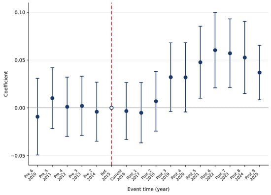
The credibility of Equation (1) rests on the counterfactual assumption that, in the absence of the Paris Agreement, treated and control firms would have followed parallel paths in cash holdings. Table 7 and Figure 1 report the event-study estimates from Equation (2). Table 7 additionally reports results using firm-level and two-way (firm and year) clustered standard errors to assess the sensitivity of statistical inference. Appendix C, Appendix D, and Appendix E (Table A3, Table A4 and Table A5) report the corresponding standard errors, t-statistics and 95% confidence intervals under each procedure.

Table 7. Event-study estimates.

Event Time	Year	(1) CASHNO	(2) CASHNO	(3) CASHNO
Pre_6	2010	−0.0092	−0.0092	−0.0092
Pre_5	2011	0.0102	0.0102	0.0102
Pre_4	2012	0.0011	0.0011	0.0011
Pre_3	2013	0.0021	0.0021	0.0021
Pre_2	2014	−0.0041	−0.0041	−0.0041
Current	2016	−0.0034	−0.0034	−0.0034
Post_1	2017	−0.0051	−0.0051	−0.0051
Post_2	2018	0.0069	0.0069	0.0069
Post_3	2019	0.0321 *	0.0321	0.0321
Post_4	2020	0.0319 *	0.0319	0.0319
Post_5	2021	0.0477 **	0.0477 **	0.0477 **
Post_6	2022	0.0604 ***	0.0604 ***	0.0604 ***
Post_7	2023	0.0571 ***	0.0571 ***	0.0571 **
Post_8	2024	0.0527 ***	0.0527 **	0.0527 **
Post_9	2025	0.0369 **	0.0369 ***	0.0369 ***
Standard Errors		Robust	Cluster (firm)	Cluster (firm, year)
Joint pre-trend test (F; p-value)		F(5, 23840) = 0.26; p = 0.9357	F(5, 1744) = 1.70; p = 0.1324	F(5, 15) = 6.89; p = 0.0016

Notes: The dependent variable is CASHNO. Coefficients are those on the interactions between TREATED and the year indicators, with 2015 omitted as the reference year. Pre_j, Current, and Post_j denote event time k = −j, 0, and j relative to 2016 (Equation (2)). All specifications include firm fixed effects, industry × year fixed effects, and the full control vector. *, **, and *** denote statistical significance at the 10%, 5%, and 1% levels, respectively.

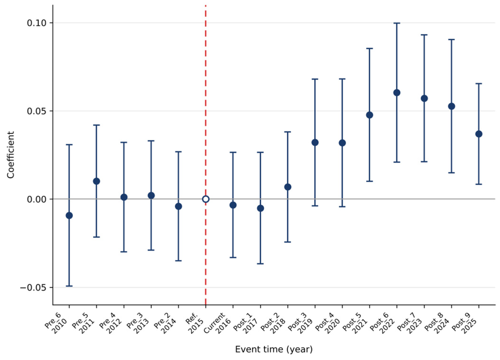
Figure 1. Event-study estimates of the effect of carbon exposure on cash holdings. Navy points are the coefficients on TREATED × year from Equation (2), and vertical bars are 95% confidence intervals based on heteroskedasticity-robust standard errors. The red vertical dashed line marks the Paris Agreement (December 2015); 2015 is the omitted reference year, with its coefficient normalised to zero. The grey horizontal line marks zero.

The pre-treatment coefficients are small in magnitude. None of the five estimable pre-event coefficients (2010 through 2014) approach conventional significance; the largest in absolute value is 0.0102 in 2011 (t = 0.63), while the remaining coefficients are also close to zero. The joint test fails to reject the null that all five pre-treatment coefficients are zero under robust standard errors (F(5, 23,840) = 0.26, p = 0.9357) and firm-level clustering (F(5, 1744) = 1.70, p = 0.1324). However, the joint test becomes significant under two-way clustering (F(5, 15) = 6.89, p = 0.0016), indicating that the evidence supporting parallel trends is sensitive to the clustering approach. Because the two-way clustered covariance matrix of the five pre-treatment coefficients is estimated from only 16 year clusters, and because the pre-treatment coefficients are individually small and show no drift toward the treatment date, we do not read this rejection as clear evidence of a differential pre-trend. Equally, the data cannot be said to confirm the parallel-trends assumption, and the event-study evidence should be interpreted with corresponding caution.

The post-treatment dynamics are more interesting than a simple step change. The coefficients for 2016, 2017, and 2018 are indistinguishable from zero. The response turns positive in 2019 (0.0321, t = 1.75) and 2020 (0.0319, t = 1.73), both significant at the 10% level under robust standard errors but insignificant under firm-level and two-way clustering. The estimated effect strengthens in 2021 (0.0477, t = 2.48) and peaks in 2022 at 0.0604 (t = 3.00). It remains positive in 2023 (0.0571), 2024 (0.0527), and 2025 (0.0369). Under robust standard errors, the 2021 and 2025 coefficients are significant at the 5% level, while those for 2022–2024 are significant at the 1% level. The coefficients from 2021 onward also remain statistically significant under both clustering approaches, although significance levels vary slightly. The delayed and persistent profile is consistent with a gradual response to the implementation of climate-policy commitments, but the single-date design cannot separate this from the initial shock of the Agreement or from other developments over the same period.

4.4. Placebo Test

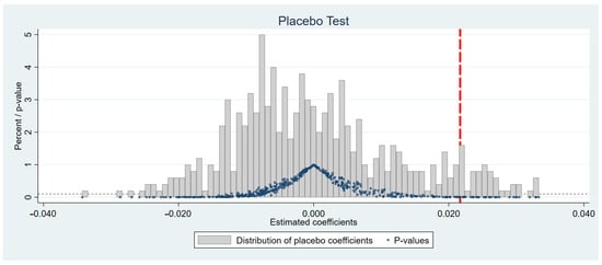
A natural concern is that the estimated effect may reflect unobserved sample-specific features rather than the treatment itself. To address this concern, we conduct a randomisation-inference placebo test. In each of 500 replications, the treatment status is randomly reassigned across firms while preserving the actual proportion of treated firms (approximately 25%, consistent with the top-quartile treatment definition). We then construct the placebo DID term by interacting the randomly assigned treatment indicator with the actual POST indicator and re-estimate Equation (1) using the same specification as in the baseline analysis. The resulting distribution of placebo coefficients is centred around zero. Of the 500 placebo replications, 48 produce coefficient estimates that are at least as extreme in absolute value as the actual DID estimate of 0.0217. Following the randomisation-inference adjustment, the corresponding empirical two-sided p-value is (48 + 1)/(500 + 1) = 0.0978. Thus, the actual estimate lies toward the upper tail of the placebo distribution, although the placebo evidence is statistically significant only at the 10% level. Figure 2 presents the distribution of placebo coefficients together with the corresponding p-values.

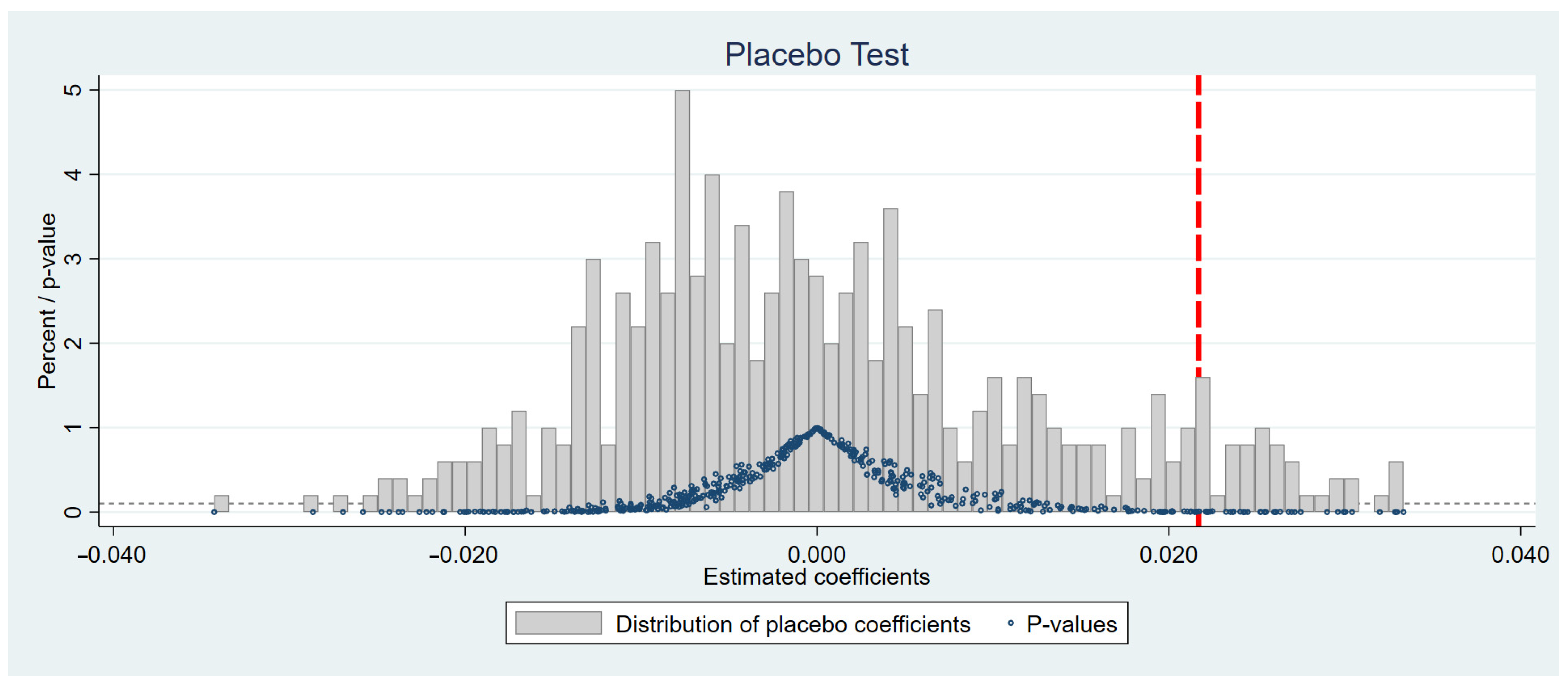
Figure 2. Placebo test. Grey bars show the distribution (in percent) of the DID coefficients across 500 replications in which treatment is randomly reassigned across firms; blue circles plot the corresponding p-values against the left axis. The red vertical dashed line marks the actual estimate of 0.0217, and the grey horizontal dashed line marks p = 0.10.

4.5. Propensity-Score-Matched Difference-in-Differences

Treated and control firms differ systematically along observable characteristics. To improve covariate comparability, we estimate the propensity score at the firm level using only pre-treatment information. Specifically, the matching covariates SIZE_TA, AGE, ROE, GRO, BOARDSIZE, LEV, CAPEXTA, BM, GDP, and CPI are averaged from 2010 to 2015, meaning that each firm contributes a single pre-treatment observation to the propensity score estimation. The treatment indicator remains determined by the firm’s carbon intensity in 2015. Treated firms are then matched one to one with control firms using nearest-neighbour matching within the common support. The matched firms are subsequently merged back into the full 2010–2025 panel on which the DiD model is re-estimated. No post-2015 information is used in the matching procedure.

Table 8 reports the balance diagnostics. Before matching, absolute standardised biases range from 0.8% to 59.5%. After matching, most covariates are closely balanced, with absolute standardised biases ranging from 0.1% to 7.8%. Although leverage retains a standardised bias of −5.9%, the difference between treated and control firms is not statistically significant (p = 0.402). The mean absolute bias falls from 23.8% to 3.1%, Rubin’s B decreases from 94.3% to 13.2%, Rubin’s R changes from 1.22 to 0.91, and the pseudo-R² of the treatment model declines from 0.136 to 0.003. The post-matching likelihood-ratio test is statistically insignificant (χ² = 3.69, p = 0.960), indicating a substantial improvement in covariate balance following matching.

Table 8. Covariate balance before and after propensity-score matching.

Variable	Sample	Treated	Control	% Bias	% Bias Red.	p-Value
SIZE_TA	Unmatched	22.925	22.634	21.4		0.000
	Matched	22.925	22.820	7.8	63.7	0.268
AGE	Unmatched	2.7728	2.8081	−8.1		0.148
	Matched	2.7728	2.7642	2.0	75.8	0.767
ROE	Unmatched	0.06850	0.13489	−35.8		0.000
	Matched	0.06850	0.06945	−0.5	98.6	0.941
GRO	Unmatched	0.04922	0.05055	−0.8		0.870
	Matched	0.04922	0.05028	−0.7	20.3	0.930
BOARDSIZE	Unmatched	2.3731	2.3174	19.2		0.001
	Matched	2.3731	2.3647	2.9	84.9	0.683
LEV	Unmatched	0.56175	0.57096	−5.1		0.364
	Matched	0.56175	0.57244	−5.9	−16.1	0.402
CAPEXTA	Unmatched	0.07513	0.04954	39.6		0.000
	Matched	0.07513	0.07521	−0.1	99.7	0.988
BM	Unmatched	0.87313	0.59188	59.5		0.000
	Matched	0.87313	0.86251	2.2	96.2	0.794
GDP	Unmatched	2.6789	2.4328	16.5		0.003
	Matched	2.6789	2.6071	4.8	70.8	0.490
CPI	Unmatched	2.4280	1.8177	32.3		0.000
	Matched	2.4280	2.3576	3.7	88.5	0.600

Notes: One-to-one nearest-neighbour propensity-score matching with replacement, imposing common support. Summary diagnostics: mean absolute standardised bias decreases from 23.8% (unmatched) to 3.1% (matched); Rubin’s B decreases from 94.3% to 13.2%; Rubin’s R changes from 1.22 to 0.91; pseudo-R² decreases from 0.136 to 0.003 (post-matching LR χ² = 3.69, p = 0.960). SIZE_TA is the natural logarithm of total assets; other variables are defined in Table 1. % Bias = standardised percentage bias; % Bias Red. = percentage reduction in absolute bias.

Re-estimating Equation (1) on the 10,180 matched firm-year observations yields a DID coefficient of 0.0309 (t = 2.39), statistically significant at the 5% level as reported in Table 9. This estimate is approximately 42.4% larger than the preferred full-sample estimate of 0.0217, but it remains positive and economically comparable. The matched result therefore supports the direction of the main finding while reducing observable differences between treated and control firms.

Table 9. Robustness checks.

Specification	(1) PSM-DiD	(2) Country × Year FE	(3) 2010–2022	(4) Excluding 2020–2021	(5) CASHAS	(6) 50th Percentile	(7) Ln(Cash)	(8) Excluding LEV, CAPEXTA, and BM
DID	0.0309 **	0.0367 **	0.0251 *	0.0286 **	0.0077 *	0.0092 **	−0.0684	0.0208 *
	(0.0129)	(0.0178)	(0.0139)	(0.0131)	(0.0046)	(0.0040)	(0.0555)	(0.0125)
	[2.39]	[2.06]	[1.80]	[2.18]	[1.70]	[2.29]	[−1.23]	[1.68]
Controls	Yes	Yes	Yes	Yes	Yes	Yes	Yes	Yes
Firm FE	Yes	Yes	Yes	Yes	Yes	Yes	Yes	Yes
Observations	10,180	25,497	21,639	22,171	25,549	25,549	25,549	25,549
Adjusted R2	0.3904	0.5174	0.4960	0.4839	0.7338	0.5083	0.8678	0.5728

Notes: Columns (1) and (3)–(8) include firm and industry-by-year fixed effects; column (2) includes firm and country-by-year fixed effects. Standard errors are two-way clustered by firm and year. Column (1) uses matched observations and matching weights. Column (6) uses the 50th-percentile treatment cut-off. Column (7) uses the natural logarithm of cash and cash equivalents as the dependent variable. Column (8) excludes leverage (LEV), capital expenditures (CAPEXTA), and the book-to-market ratio (BM) to assess sensitivity to potential post-treatment controls. Standard errors are in parentheses ( ), and t-statistics are in square brackets [ ]. * and ** indicate significance at the 10% and 5% levels, respectively. PSM-DiD = propensity-score-matched difference-in-differences; FE = fixed effects; other variables are defined in Table 1.

4.6. Additional Robustness Checks

Table 9 reports the matched estimate together with seven additional robustness checks.

Country-by-year fixed effects. The most serious threat to identification is that treated and control firms are unevenly distributed across countries whose climate and macroeconomic policies diverged after 2015. Replacing year fixed effects with country × year fixed effects absorbs country-specific time-varying shocks. Under this demanding specification, the DID coefficient is 0.0367 (t = 2.06), significant at the 5% level with two-way clustered standard errors. The estimate is about 69.1% larger than the preferred coefficient of 0.0217, suggesting that the positive coefficient is not driven by cross-country composition.

Shorter window. Restricting the sample to 2010–2022 removes the three most recent years. The DID coefficient is 0.0251 (t = 1.80), which remains positive and statistically significant at the 10% level and is approximately 15.7% larger than the preferred estimate of 0.0217.

Excluding the pandemic. Because the estimated effect strengthens around the COVID-19 period, an alternative explanation is that carbon-intensive firms simply hoarded cash more aggressively during the liquidity shock. Dropping 2020 and 2021 yields a DID coefficient of 0.0286 (t = 2.18), significant at the 5% level. This estimate is approximately 31.8% larger than the preferred coefficient of 0.0217, suggesting that the pandemic years do not generate the main result.

Alternative dependent variable. Replacing CASHNO with CASHAS, the ratio of cash to total assets, yields a coefficient of 0.0077 (t = 1.70), which is significant at the 10% level. Relative to the CASHAS sample mean of 0.1151, this corresponds to an increase of approximately 6.7%. The coefficient therefore remains positive under the alternative scaling of cash holdings, although its statistical significance is weaker.

Alternative treatment cut-off. Column (6) redefines treatment using the 50th percentile of the 2015 carbon intensity distribution rather than the baseline 75th-percentile cut-off. The DID coefficient remains positive at 0.0092 (t = 2.29) and is statistically significant at the 5% level. Although the estimate is approximately 57.6% smaller than the preferred coefficient of 0.0217, the positive and statistically significant result suggests that the main finding is not driven solely by the top-quartile treatment threshold.

Level of cash. Because CASHNO has non-cash assets in the denominator, a higher ratio could reflect slower growth in non-cash assets rather than additional cash. We therefore re-estimate the preferred specification with the natural logarithm of cash and cash equivalents as the dependent variable. The DID coefficient is −0.0684 (t = −1.23) and is not statistically significant. Because the level of cash does not rise, the higher cash ratio may reflect slower growth in non-cash assets rather than additional cash. We therefore describe the main result as a relative rise in the cash ratio rather than as an accumulation of cash.

Excluding potential post-treatment controls. Leverage, capital expenditures, and the book-to-market ratio are included in the baseline as standard determinants of cash holdings (Opler et al., 1999; Bates et al., 2009) to control for differences in financial structure, investment and valuation. Because deleveraging and changes in asset allocation are themselves possible responses to the post-Paris environment, these contemporaneous controls may absorb part of the effect. Column (8) therefore re-estimates the preferred specification without them. The DID coefficient is 0.0208 (t = 1.68), significant at the 10% level, and is nearly identical to the preferred estimate of 0.0217, which indicates that the three controls absorb little of the estimated effect.

4.7. Exploratory Mediation Analysis

Table 10 reports the mediation analysis using the financial constraints index of Whited and Wu (2006) (WW index). The results show that DID is positively associated with WW (a = 0.0049, p < 0.01), while WW is positively associated with CASHNO conditional on DID (b = 1.4803, p < 0.01). The estimated indirect effect is positive (0.0072) and statistically significant at the 1% level, accounting for approximately 33.4% of the total effect (0.0217). In contrast, the direct effect (0.0144) is not statistically significant.

Table 10. Mediation analysis: the financing-constraints channel.

	WW Index
	Coefficient	Std. Error
Path a: DID → Mediator	0.0049 ***	(0.0010)
Path b: Mediator → CASHNO	1.4803 ***	(0.3177)
Indirect effect (a × b)	0.0072 ***	(0.0025)
Direct effect	0.0144	(0.0117)
Total effect	0.0217 *	(0.0125)
Proportion mediated	0.3338	(5.3385)
Bootstrap replications	500
Observations	25,549

Notes: All specifications include firm fixed effects, industry-by-year fixed effects, and the full set of control variables. Standard errors are two-way clustered at the firm and year levels. The indirect effect and the proportion mediated are estimated using 500 bootstrap replications. * and *** indicate statistical significance at the 10% and 1% levels, respectively. WW = Whited and Wu (2006) financial constraints index; other variables are defined in Table 1.

However, the estimated proportion mediated should be interpreted cautiously. Its bootstrap standard error is substantial (5.3385), while the total effect is statistically significant only at the 10% level. Moreover, identifying a causal mediation effect requires strong assumptions that may not hold for the WW index, which is constructed from multiple firm-level financial characteristics, including cash flow, dividend policy, leverage, firm size, and sales growth. Accordingly, the results are interpreted as exploratory evidence that changes in measured financial constraints accompany the post-Paris relative increase in corporate cash ratios, rather than as conclusive evidence of a causal mediation mechanism.

5. Discussion

5.1. Interpreting the Main Effect

The central result is that, after the Paris Agreement, the cash ratios of carbon-intensive firms rose relative to those of less carbon-intensive peers in the same industry and year. The point estimate—roughly 15% of the average cash ratio—is economically meaningful and plausible as a cumulative adjustment over several years, although it is not accompanied by an increase in the level of cash. The event-study profile shows no differential change in 2016–2018 and a relative rise from 2019 onward. One plausible reading is that national implementation, disclosure frameworks and investor pressure gradually gave the commitment operational content. Our single-date design, however, cannot separate the initial shock of the Agreement from this later implementation or from other developments over the same period, so the timing is consistent with, but does not establish, a response to implementation rather than to the announcement.

This interpretation relates our findings to the policy-uncertainty branch of the cash-holdings literature. Phan et al. (2019) and Duong et al. (2020) showed that generic policy uncertainty raises corporate cash, and recent studies link climate risk and the Paris Agreement to higher cash holdings (Wu et al., 2025; Tran et al., 2025; Wang et al., 2026). Our estimates are consistent with this evidence. Because the incidence of climate-policy uncertainty varies with a measurable pre-event characteristic, carbon intensity, it can be studied with a difference-in-differences design; we do not claim this feature as a contribution of the present study.

The result also complements the capital-structure evidence. Nguyen and Phan (2020) documented that carbon-risk exposure reduces leverage. Our finding is consistent with a broader balance-sheet adjustment in which the share of cash in the assets of carbon-intensive firms rises relative to peers. Because the level of cash does not increase, this adjustment may reflect slower growth in non-cash assets rather than additional cash.

5.2. Interpreting the Constraints Channel

The mediation results indicate that the post-Paris period is associated with higher values of the WW financial constraints index (Whited & Wu, 2006) among treated firms, and that higher WW values are positively associated with corporate cash ratios. The estimated indirect effect is positive and statistically significant, accounting for approximately 33.4% of the total effect. However, this proportion is imprecisely estimated, and the total effect itself is statistically significant only at the 10% level. These findings are consistent with a precautionary-liquidity interpretation, but do not establish that financing constraints causally drive the observed relative increase in cash ratios.

The WW index combines cash flow, dividend status, long-term debt, firm size, industry sales growth, and firm sales growth. Because it is a composite measure rather than a direct observation of credit availability, changes in the index may partly reflect broader adjustments in firms’ financial characteristics. Moreover, causal mediation analysis requires strong identification assumptions that cannot be fully verified in the present setting. Accordingly, the estimated indirect effect should be interpreted as exploratory evidence consistent with a financing-constraints channel rather than as a structural causal parameter.

We therefore treat Table 10 as suggestive evidence that changes in measured financing constraints accompany the post-Paris relative increase in corporate cash ratios. A more direct test would compare the estimated treatment effects across firms with different levels of financial constraints measured before 2016. Establishing the mechanism more convincingly would require complementary indicators, such as credit ratings, credit-line availability, loan spreads, or other market-based measures of external financing conditions. These measures provide a useful direction for future research.

5.3. Limitations

Five limitations bound the interpretation. First, the sample is restricted to firms with carbon data before 2016 and non-missing carbon intensity in 2015, which may tilt the estimation sample toward larger and more transparent issuers; the estimated effect therefore applies to firms for which pre-treatment carbon exposure can be identified rather than to the full population of listed firms. Second, emissions data are measured with error. Aswani et al. (2024) showed that vendor-estimated emissions differ systematically from disclosed figures and are highly correlated with financial fundamentals. To the extent that estimated values enter treatment assignment, the error is unlikely to be classical, so it need not bias the estimates toward zero and could bias them in either direction. Third, the Paris Agreement was not the only global shock in the post-2015 window; while country × year and industry × year fixed effects and the exclusion of the pandemic years mitigate this concern, they cannot rule out every contemporaneous shock with an emissions-correlated incidence. Fourth, the DiD estimand is a relative effect. We identify how carbon-intensive firms changed their behaviour relative to peers, not the level effect of the Agreement on aggregate corporate liquidity, and because the outcome is a ratio, the estimate describes a relative change in the cash ratio. Fifth, two-way clustered inference rests on only 16 year clusters. The joint pre-trend test rejects the null under this procedure but not under robust or firm-clustered standard errors, so the support for the parallel-trend assumption depends on the inference procedure, and the evidence should be regarded as suggestive rather than conclusive.

5.4. Implications

For investors, the finding suggests that carbon-intensive firms carry relatively higher cash ratios after the Paris Agreement, which may matter for valuation multiples and for the interpretation of return spreads. For lenders and credit analysts, a rising cash ratio among carbon-intensive borrowers may signal anticipated transition costs, although our evidence does not show that these borrowers hold more cash in absolute terms. For policymakers, the delayed onset of the differential response is suggestive: if it reflects implementation, framework commitments may change behaviour mainly once they are translated into instruments with dates and prices attached, although our design cannot confirm this. For managers and boards, the results suggest that transition risk may bear on liquidity management and on disclosure.

6. Conclusions

Using the Paris Agreement as a shock to the salience of climate-transition risk, this paper finds thatin our preferred specification with firm fixed effects, industry-by-year fixed effects, and standard errors two-way clustered by firm and year, the cash-to-net-assets ratio of carbon-intensive firms rises by approximately 2.17 percentage points relative to less carbon-intensive peers. This magnitude is approximately 14.9% of the full-sample mean and is statistically significant at the 10% level. The pre-treatment event-study coefficients are small and individually insignificant, but their joint test rejects the null under two-way clustering, so the support for parallel pre-trends depends on the inference procedure; the post-treatment profile becomes positive from 2019 and persists through 2025. The placebo test places the actual estimate toward the upper tail of the randomisation distribution (empirical two-sided p = 0.0978), and the coefficient remains positive under propensity-score matching, country × year fixed effects, the exclusion of the pandemic years, an alternative cash measure, a 50th-percentile treatment cut-off, and the exclusion of potential post-treatment controls, although several of these estimates are only marginally significant. The level of cash does not rise, so the result concerns the cash ratio rather than the accumulation of cash. An exploratory decomposition shows that the WW financing-constraints index moves with cash ratios, but it does not establish a causal mediating channel. Because the design cannot separate the Agreement from later implementation and other post-2015 developments, the evidence is best read as suggestive of an association between the post-Paris transition-policy environment and a relative rise in the cash ratios of carbon-intensive firms.

The broader message is that the post-Paris climate-policy environment may be associated with changes in corporate liquidity management. Future research should extend the analysis in three directions: examining whether the higher cash ratios reflect changes in cash itself or in non-cash assets, such as reduced investment; exploiting within-country variation in carbon-pricing stringency to sharpen the policy interpretation; and testing whether the marginal value of cash differs for carbon-intensive firms in the way that a precautionary account would predict.

References

- Almeida, H., Campello, M., & Weisbach, M. S. (2004). The cash flow sensitivity of cash. The Journal of Finance, 59(4), 1777–1804. [Google Scholar] [CrossRef] [Scilit]
- Aswani, J., Raghunandan, A., & Rajgopal, S. (2024). Are carbon emissions associated with stock returns? Review of Finance, 28(1), 75–106. [Google Scholar] [CrossRef] [Scilit]
- Bartram, S. M., Hou, K., & Kim, S. (2022). Real effects of climate policy: Financial constraints and spillovers. Journal of Financial Economics, 143(2), 668–696. [Google Scholar] [CrossRef] [Scilit]
- Bates, T. W., Kahle, K. M., & Stulz, R. M. (2009). Why do U.S. firms hold so much more cash than they used to? The Journal of Finance, 64(5), 1985–2021. [Google Scholar] [CrossRef] [Scilit]
- Bertrand, M., Duflo, E., & Mullainathan, S. (2004). How much should we trust differences-in-differences estimates? The Quarterly Journal of Economics, 119(1), 249–275. [Google Scholar] [CrossRef] [Scilit]
- Bolton, P., & Kacperczyk, M. (2021). Do investors care about carbon risk? Journal of Financial Economics, 142(2), 517–549. [Google Scholar] [CrossRef] [Scilit]
- Bolton, P., & Kacperczyk, M. (2023). Global pricing of carbon-transition risk. The Journal of Finance, 78(6), 3677–3754. [Google Scholar] [CrossRef] [Scilit]
- Cameron, A. C., Gelbach, J. B., & Miller, D. L. (2011). Robust inference with multiway clustering. Journal of Business & Economic Statistics, 29(2), 238–249. [Google Scholar] [CrossRef] [Scilit]
- Cameron, A. C., & Miller, D. L. (2015). A practitioner’s guide to cluster-robust inference. Journal of Human Resources, 50(2), 317–372. [Google Scholar] [CrossRef] [Scilit]
- Correia, S. (2016). A feasible estimator for linear models with multi-way fixed effects (Working Paper). Duke University. Available online: http://scorreia.com/research/hdfe.pdf (accessed on 12 October 2026).
- Delis, M. D., de Greiff, K., Iosifidi, M., & Ongena, S. (2024). Being stranded with fossil fuel reserves? Climate policy risk and the pricing of bank loans. Financial Markets, Institutions & Instruments, 33(3), 239–265. [Google Scholar] [CrossRef] [Scilit]
- Denis, D. J., & Sibilkov, V. (2010). Financial constraints, investment, and the value of cash holdings. The Review of Financial Studies, 23(1), 247–269. [Google Scholar] [CrossRef] [Scilit]
- Duong, H. N., Nguyen, J. H., Nguyen, M., & Rhee, S. G. (2020). Navigating through economic policy uncertainty: The role of corporate cash holdings. Journal of Corporate Finance, 62, 101607. [Google Scholar] [CrossRef] [Scilit]
- Ginglinger, E., & Moreau, Q. (2023). Climate risk and capital structure. Management Science, 69(12), 7492–7516. [Google Scholar] [CrossRef] [Scilit]
- Han, S., & Qiu, J. (2007). Corporate precautionary cash holdings. Journal of Corporate Finance, 13(1), 43–57. [Google Scholar] [CrossRef] [Scilit]
- Ilhan, E., Sautner, Z., & Vilkov, G. (2021). Carbon tail risk. The Review of Financial Studies, 34(3), 1540–1571. [Google Scholar] [CrossRef] [Scilit]
- Javadi, S., & Masum, A.-A. (2021). The impact of climate change on the cost of bank loans. Journal of Corporate Finance, 69, 102019. [Google Scholar] [CrossRef] [Scilit]
- Krueger, P., Sautner, Z., & Starks, L. T. (2020). The importance of climate risks for institutional investors. The Review of Financial Studies, 33(3), 1067–1111. [Google Scholar] [CrossRef] [Scilit]
- Nguyen, J. H., & Phan, H. V. (2020). Carbon risk and corporate capital structure. Journal of Corporate Finance, 64, 101713. [Google Scholar] [CrossRef] [Scilit]
- Opler, T., Pinkowitz, L., Stulz, R., & Williamson, R. (1999). The determinants and implications of corporate cash holdings. Journal of Financial Economics, 52(1), 3–46. [Google Scholar] [CrossRef] [Scilit]
- Phan, H. V., Nguyen, N. H., Nguyen, H. T., & Hegde, S. (2019). Policy uncertainty and firm cash holdings. Journal of Business Research, 95, 71–82. [Google Scholar] [CrossRef] [Scilit]
- Preacher, K. J., & Hayes, A. F. (2008). Asymptotic and resampling strategies for assessing and comparing indirect effects in multiple mediator models. Behavior Research Methods, 40(3), 879–891. [Google Scholar] [CrossRef] [Scilit] [PubMed]
- Seltzer, L. H., Starks, L. T., & Zhu, Q. (2022). Climate regulatory risk and corporate bonds (NBER Working Paper No. 29994). National Bureau of Economic Research. [CrossRef] [Scilit]
- Tran, L. T. H., Trinh, V. Q., Le, V. T. P., & Tu, T. T. K. (2025). Carbon emissions, firm-level climate change exposure, and corporate cash reserves. Business Strategy and the Environment, 34(5), 5158–5180. [Google Scholar] [CrossRef] [Scilit]
- Wang, Y., Kong, D., & Xu, M. (2026). Climate risk perception and corporate responses under the Paris agreement: Evidence from firms’ cash holdings. Accounting & Finance, 66(3), 2807–2821. [Google Scholar] [CrossRef] [Scilit]
- Whited, T. M., & Wu, G. (2006). Financial constraints risk. The Review of Financial Studies, 19(2), 531–559. [Google Scholar] [CrossRef] [Scilit]
- Wu, Z., Shih, Y. C., Wang, Y., & Zhong, R. (2025). The effects of decarbonization on corporate cash holdings. Emerging Markets Review, 69, 101356. [Google Scholar] [CrossRef] [Scilit]
Disclaimer/Publisher’s Note: The statements, opinions and data contained in all publications are solely those of the individual author(s) and contributor(s) and not of MDPI and/or the editor(s). MDPI and/or the editor(s) disclaim responsibility for any injury to people or property resulting from any ideas, methods, instructions or products referred to in the content. |
© 2026 by the authors. Licensee MDPI, Basel, Switzerland. This article is an open access article distributed under the terms and conditions of the Creative Commons Attribution (CC BY) license.