


Abstract
Language models can translate mathematical prose into formal statements and produce machine-checked proofs, and they are increasingly used in finance. Such a proof, however, certifies the model as written, not the model intended. In dynamic finance the difference concerns information: a position must be chosen using only what is known when it is taken, and an exercise decision cannot depend on prices not yet observed. A formalization that allows more information than the model specifies can be proved correct and still be financially inadmissible. We show that auditing realized outcomes cannot detect such errors: one realized history is consistent with exponentially many patterns of look-ahead, while two scenarios suffice to expose one. We build the model’s information structure into the formalization procedure, so that every intermediate quantity provably uses only information available at its date, and verify the main theorems in Lean 4. On 2960 synthetic instances, removing only the information rules lowers certified success by 19.8 percentage points, and the procedure then declares 91.5% of look-ahead errors valid. When the model is read from prose, the main residual error is a timing convention the text never states; in an exploratory experiment, requiring a verbatim quotation for each convention eliminated it.
1. Introduction
Language models have become capable enough to translate mathematical prose into the syntax of a proof assistant and to search for proofs of the resulting statements (First et al., 2023; Jiang et al., 2023; Y. Wu et al., 2022; Yang et al., 2023), and in restricted domains they now produce proofs at a level that was recently out of reach (Trinh et al., 2024). At the same time, language models are being adopted across quantitative finance (Li et al., 2023; S. Wu et al., 2023). The natural combination—having a model read a description of a market, formalize it, and prove that a proposed trading or exercise rule is sound—is attractive precisely because the proof assistant appears to remove the need to trust the model.
It does not, and the reason is specific to dynamic finance. A proof assistant certifies the statement it is given about the model it is given. If the formalization silently enlarges the information available at a date, weakens predictability to adaptedness, shifts the convention that fixes when a position is chosen, or substitutes the physical measure for the pricing measure, then the resulting theorem is true and the financial claim is false. In a static valuation problem such errors are arithmetic and usually visible in the numbers. In a dynamic one they are informational: an admissible object must be measurable with respect to the filtration that describes what is known when it is formed (Föllmer & Schied, 2016; Harrison & Kreps, 1979; Harrison & Pliska, 1981), and a violation of that requirement need not disturb any number the model produces.
Consider a trading rule that fixes the position for after seeing , a stopping rule that consults information revealed only after it claims to stop, or a value process that satisfies the terminal identity but not the local ones at intermediate nodes. Each is inadmissible in the model. Each can nevertheless reproduce a plausible profit and loss series, and some reproduce the exact numbers of a legitimate rule. The practical importance of this failure mode is well documented: backtest overfitting and its statistical consequences have been analyzed at length (Bailey et al., 2014; Harvey et al., 2016), and the literature on quantitative practice treats look-ahead contamination as a first-order source of model risk (López de Prado, 2018). What has been missing is a statement of how much of this contamination is detectable in principle from realized data, and a formalization procedure whose guarantees do not depend on the analyst noticing the problem.
This paper contributes both. Section 4 proves that validating an autoformalized model against its own output cannot detect such errors: given a predictable strategy and a realized path, one can construct exponentially many strategies with identical realized holdings, wealth and returns along that path whose sets of measurability failures are pairwise distinct. Any audit that reads only the realized record therefore returns the same verdict on a legitimate strategy and on a contaminated one. A second result shows that a refutation needs at least two terminal paths, so the two-path witness produced by our method is the smallest possible.
The positive contribution is a formalization procedure that treats the filtration as a specification rather than as a hypothesis. We say that the filtration is compiled into the procedure because, before any reasoning starts, it is turned into the structure of the procedure: for each distinct information state a slice of up to three components (forward, backward and reconciliation), and for each component a rule stating which objects it may read. Objects carry the date of the information they depend on, components exchange them only as messages that record this date, and information about the future may reach an earlier decision only as a conditional expectation given what is known at that decision. Under these rules non-anticipativity becomes a property of the protocol. Theorems 3 and 4 show that whatever a date-t component computes from legal inputs is -measurable, with no analysis of the computation itself and no assumption about the behavior of the language model that proposed the formalization. Theorems 6 and 7 supply the tower property in the finite setting and compose one-period identities into the global pricing identity, and Theorem 5 shows that one slice per distinct information state is the fewest any admissible decomposition can use. Figure 1 shows the procedure from prose to verified verdict.
Figure 1.
The procedure from prose to verified verdict. A language model reads the specification and proposes the timing conventions and the model; a convention is admitted only together with a verbatim quotation from the source, and is otherwise marked as unstated (Section 11.3). After structural checks, the filtration compiler builds one slice of components per information state, and the exact core verifies the obligation with a forward and a backward pass over dates, a reconciliation at each date, and the message rules of Section 5. The result is a verdict with a certificate, or with a witness of the violation, which the Lean kernel checks again. If the verdict depends on a convention that the source leaves open, the procedure abstains and names the missing convention. Nothing above the dashed line is trusted; below it, the verdicts of the exact core are confirmed by the Lean kernel, the only part whose acceptance counts as a proof.
Every theorem stated below, apart from two counting corollaries, is verified in Lean 4 (de Moura & Ullrich, 2021) using only its core library. Instance data are carried as unnormalized pairs of integers, on which all operations reduce inside the kernel, and proved bridge lemmas transfer the resulting statements to the rational numbers; no computation outside the kernel is relied on. The language model sits entirely outside this trusted part: it proposes a formalization, and nothing it produces is accepted until the exact core—the part of the procedure that checks the obligations in exact rational arithmetic—verifies it, the information rules admit it and the kernel accepts the certificate.
The empirical part uses 2960 synthetic instances with exact rational data and addresses two separate questions. Section 10 asks whether the procedure verifies a model that is supplied to it, and isolates the contribution of the information rules. Section 11 asks what happens when a language model must first recover the model from prose, and tests the conclusions on five language models. There the dominant residual error is not a misread number but a timing convention that the text never states and the language model nevertheless supplies. In an exploratory experiment, a grounding constraint that admits a convention only when the language model quotes the sentence stating it removes these errors: the procedure then abstains on every under-determined specification and states which convention is missing.
Section 3 fixes the setting and the scope of the framework, Section 4, Section 5, Section 6 and Section 7 develop the theory, and Section 8 presents the formal development. Section 9 sets out the benchmark and the experimental design, Section 10 and Section 11 report the results, and Section 12, Section 13 and Section 14 give case studies, a discussion and conclusions. Appendix A lists the prompts and model settings, and Appendices Appendix B and Appendix C give additional results.
2. Related Work
The problem sits where several bodies of literature meet, each of which supplies part of the picture while leaving the informational question open.
- Autoformalization and machine-checked proof.
Translating mathematical prose into the language of a proof assistant, and searching for proofs of the result, has advanced quickly (First et al., 2023; Jiang et al., 2023; Polu & Sutskever, 2020; Y. Wu et al., 2022; Yang et al., 2023), to the point of competitive performance in restricted domains (Trinh et al., 2024). The benchmarks that drive this work are drawn from competition problems and from formal libraries such as mathlib (The Mathlib Community, 2020), where the statement to be proved is supplied and the difficulty lies in finding the proof. Evaluation is correspondingly proof-centric: a formalization is counted as correct when the kernel accepts it. That is the criterion this paper argues is insufficient for dynamic financial models, where a kernel-accepted proof of a subtly misspecified statement is the characteristic failure rather than an exception. The reverse direction—checking that a formal statement says what the informal one said—is recognized as the weak link, and is usually addressed by human inspection or by translating the formal statement back into prose. Neither helps here: the discrepancies that matter are invisible in the numbers a model produces, by Theorem 1.
- Formal methods for numerical and financial computation.
Formalizing analysis in a proof assistant is by now well developed, and surveys of that effort make clear where the weight has fallen: on real and floating-point arithmetic and on the libraries needed to reason about it (Boldo et al., 2016). Verification of numerical software inherits that emphasis, asking whether an implementation stays within a stated bound of its real-arithmetic specification, and taking the specification itself as given. The errors studied here are of the opposite type. They occur in the specification, they are exact rather than approximate, and they leave the computed numbers untouched. Our use of exact rational arithmetic is therefore not a sharpening of numerical error control but a way of making a residual into a certificate; Section 10 separates the two effects experimentally.
- Look-ahead and backtest validity.
That trading rules can be contaminated by information they should not have is well known in quantitative practice. The statistical literature quantifies the consequences of selecting a strategy on the same data used to evaluate it (Bailey et al., 2014; Harvey et al., 2016), and treats look-ahead as a first-order source of model risk (López de Prado, 2018). The instruments are inferential: deflated performance measures, multiple-testing corrections, out-of-sample protocols. All of them take the strategy as given and ask whether its measured performance is real. The prior question—whether the strategy is an admissible object of the model at all—is not one that realized performance can answer, and Corollary 1 explains why: contamination and legitimacy are compatible with the same record.
- Language-model systems for finance.
Domain-adapted language models and multi-component systems are being applied across financial analysis (Li et al., 2023; S. Wu et al., 2023), and are evaluated by agreement with reference answers. Such a measure cannot detect an informationally inadmissible intermediate step, because the reference answer records the conclusion, not the information used to reach it. The procedure proposed here also consists of several components, but they are indexed by the dates of a filtration, and what governs their communication is a measurability constraint rather than a workflow.
- Mathematical foundations.
The mathematics we formalize is classical (Cox et al., 1979; Delbaen & Schachermayer, 1994; Föllmer & Schied, 2016; Harrison & Kreps, 1979; Harrison & Pliska, 1981; Neveu, 1975; Peskir & Shiryaev, 2006; Snell, 1952). Our contribution is not to this theory but to its use as a specification: the filtration, which in the classical treatment is a hypothesis under which theorems are stated, becomes here a constraint that a verification procedure enforces on itself.
3. Discrete-Time Setting
3.1. Event Trees and Filtrations
Let be a finite rooted tree with root r, level map , and . For with let denote its children, and assume . Each edge carries a strictly positive rational transition probability with . The terminal level is the path space; for we write
and for we write for the unique node of on its path and . The partitions generate the filtration , and because every element of is a union of elements of . Since is a finite partition that generates , a map is -measurable exactly when it is constant on each cell , . We use this characterization throughout and never require more of the underlying measure theory. Measurability is stated for vector-valued maps because the holdings and prices of d assets are vectors in ; conditional expectations are defined below for scalar maps and applied componentwise to vectors.
The pricing measure on is , and for we write . Because all transition probabilities are strictly positive, for every t and , and the conditional expectation of is the exact rational quantity
When X is -measurable, (1) reduces to the familiar one-step average over the children of , where denotes the common value of X on . We work with (1) because it is defined for arbitrary X and because it is the form in which the tower property is established in Section 6.
3.2. Obligations
Fix d risky assets with discounted prices , adapted by construction, and a numeraire normalization fixed once for the model. Conditions stated for vector-valued objects are understood componentwise, and and denote the components for asset a. We adopt the convention that the position recorded for the interval is chosen at date t. A trading strategy is a family of maps , where the index names the interval over which the position is held, not the date at which it is chosen. This representation does not build measurability into the object, so predictability is a property to be verified rather than an assumption. The obligations we consider are the following.
Definition 1.
Let be a process, H a strategy, V a wealth process, G a terminal payoff, an adapted exercise payoff, and a random time.
- (i)
- X is adapted if is -measurable for every t.
- (ii)
- H is predictable if is -measurable for every .
- (iii)
- V is self-financing for H if for all and ,
- (iv)
- S is a Q-martingale if for all and ω.
- (v)
- Y is the value process of G if and for .
- (vi)
- Z is the Snell envelope of if and for .
- (vii)
- τ is a stopping time if for all t.
Each obligation admits a short certificate in both directions. In the affirmative direction the certificate is the collection of local identities; in the negative direction it is a finite witness, and Section 7 shows that such a witness always exists and identifies the earliest date at which the model is already inconsistent.
3.3. Scope and Assumptions
The framework rests on the following assumptions, and every guarantee below holds under them.
- (a)
- Time is discrete and the horizon T is finite.
- (b)
- Uncertainty is described by a finite tree whose transition probabilities are strictly positive rationals. They are the probabilities of the pricing measure Q stated in the model, and prices are discounted by a numeraire fixed in the model.
- (c)
- Information is described by a filtration given as a sequence of partitions of the path space: the one generated by the tree, or, when the model says so, a coarser or finer one specified explicitly.
- (d)
- Markets are frictionless: there are no transaction costs, position limits or solvency constraints.
- (e)
- The obligations are those of Definition 1.
Within these assumptions the procedure decides each obligation exactly and returns a certificate in either direction.
Its guarantees are relative to the model it verifies. If the language model recovers the wrong model—a mistyped price, a misread information structure, a wrong measure—the procedure verifies the wrong model, and the information rules enforce the wrong filtration; Section 11 measures how often this happens. The procedure checks that discounted prices are martingales under the stated measure, but not whether that measure is the right one for the market at hand (Section 13 returns to this point). It does not estimate a model from data, and it covers continuous-time models only through their discretizations. Finally, the benchmark of Section 9 is synthetic: its results describe performance on constructed problems with known answers, not on specifications written by practitioners.
4. Blindness of Outcome-Based Auditing
We first make precise what an audit based on realized data can see. Fix a strategy H, an initial wealth , and let denote the wealth process generated by (2) from . For a realized path the observational record is
This contains the realized price path, the realized holdings, the realized wealth path and hence the realized period returns and terminal wealth: everything an audit of the realized history can observe.
Lemma 1.
If for every , then for every , and consequently .
Proof.
Induction on t. Both processes start at . Suppose they agree at date t along . Evaluating (2) at , the two increments depend on the strategy only through and , which coincide, and the prices are the same in both cases; so the processes agree at . □
The lemma already says that the record depends on the strategy only through its values on the single realized path. The next theorem turns this into a quantitative obstruction; Figure 2 illustrates its construction on a three-period tree. Write
the set of dates at which the realized path has not yet been separated from every other path. Since , the set is an initial segment .
Figure 2.
The construction of Theorem 1 on a three-period tree. The realized path is drawn in bold. At date 1 the strategy may not distinguish from any other path in the cell ; perturbing the holding at alone therefore breaks -measurability while leaving every quantity observed along unchanged. Doing this independently at each date in produces strategies with the same observational record.
Theorem 1
(Observational indistinguishability). Let H be predictable, let , fix an asset index a, a scalar , and for each a path . For define by
where is the a-th unit vector. Then
- (i)
- for every and hence, ;
- (ii)
- the set of dates t at which fails to be -measurable is exactly D.
In particular, the strategies with are pairwise distinct in their sets of measurability failures and all share the observational record of the predictable strategy H.
Proof.
For (i), note that for every , so the indicator in (4) vanishes at ; Lemma 1 then gives the equality of records.
For (ii), let . Both and lie in , and since H is predictable, . Therefore,
so is not constant on and hence not -measurable. Conversely, if then , which is -measurable because H is predictable. Distinctness of the for distinct D follows because their failure sets are distinct. □
Corollary 1
(Audit blindness). Let A be any map assigning to an observational record one of the two verdicts admissible and inadmissible. Then for every predictable H, every and every nonempty , the map A returns the same verdict on H and on , and is therefore incorrect on at least one of the two. In particular, on a family of such pairs the fraction of pairs on which A is correct on both members is zero.
Proof.
By Theorem 1(i) the two records coincide, so A returns the same verdict; by (ii) exactly one of the two strategies is predictable. □
Corollary 2
(Exponential ambiguity). If has at least two children for every , then and a single observational record is compatible with distinct nonempty patterns of measurability failure.
Proof.
Fix . By hypothesis has two distinct children . Every node of a finite tree with for all non-terminal v has at least one terminal descendant, so and are nonempty; they are disjoint because lie at the same level. Since we get , whence and . □
The obstruction is not an artifact of allowing arbitrary perturbations: it persists when the modification is restricted to a single asset, a single alternative path per date and an arbitrarily small . It is a statement about which functions of the model the realized record determines. Figure 3 shows how the gap grows with the horizon.
Figure 3.
The gap opened by Theorem 1, on trees in which every non-terminal node branches, so that . The number of distinct nonempty patterns of measurability failure, (labeled at each horizon), is compared with the number of observational records they produce, which is one: an audit that reads the record sees the same record for all of them. Circles mark horizons at which the family was enumerated exhaustively and the count confirmed.
The dual question is how large a certificate must be in order to refute predictability. Two paths are necessary, and two always suffice.
Theorem 2
(Optimal refutation size). For every strategy H and every there exists a predictable strategy with for all . Consequently, if R is a predicate of the restriction of H to a single path and R implies that H is not predictable, then R is never satisfied: no single-path certificate can refute predictability.
Proof.
Define if and otherwise. If then either both cells equal or neither does, so takes the same value at and ; hence, is predictable. Taking gives . For the second claim, suppose R held for some H at . Since R depends only on the restriction to , it would also hold for , and would then imply that the predictable strategy is not predictable, a contradiction. □
A pair with and refutes predictability and uses exactly two paths, and by Theorem 2 no certificate that mentions a single path can refute it. This is the sense in which the size is optimal: a two-path witness mentions the fewest terminal paths that any refutation can. The verification method of the next section produces this certificate, together with the date t, and Section 7 shows that the date it reports is the earliest one at which the model is inconsistent.
5. Information Discipline
Theorem 1 shows that the information content of a decision object cannot be recovered from what the model produces; it must be tracked while the model is built. We do so by attaching to every intermediate object the information set relative to which it is measurable, and by restricting how objects may be combined.
Objects are -valued; vector-valued objects are treated componentwise. We distinguish three kinds. A model object is a description of the model itself: the tree, the transition kernel, the price functions, the payoff definitions. Such a description does not depend on which path is realized, so as a function on it is constant and its scope—the date of the information it depends on—is 0; reasoning about it is legitimate at any date, because a proof quantifies over all paths. A realized object represents information disclosed along a particular history and carries as its scope the index t of the coarsest that makes it measurable. Evaluating a model object along the realized path does not preserve its kind: the result is a realized object, with the scope its measurability dictates. A derived object is produced from other objects by one of the admissible operators below, and carries both its scope and the operator that produced it. The distinction between model and realized objects prevents a common conflation: that a proof may inspect the entire model does not entitle a trading rule to observe the entire model.
Five operators are admissible. The forward lift for leaves an object unchanged and only weakens its measurability claim. The conditional projection sends X to , and the dynamic-programming step sends to . A join combines objects only when their measure, numeraire, date convention and node identifiers agree. Finally, a stopped process may be disclosed once the underlying random time has been shown to be a stopping time. Each operator produces an object whose scope is determined by its inputs, and the result records which operator produced it.
The compiled procedure attaches to each information state t a slice of up to three components (Figure 4); which of them are present depends on the checks the obligation requires. Three further components, for the model specification, the checking of messages and the compilation of certificates, serve all slices, and auxiliary components may be created on demand at a node where a violation is detected. A forward component checks the obligations that concern decisions taken at date t, such as the measurability of the position chosen at t; taken together, the forward components make a forward pass over the dates. A backward component computes values at date t from values at , as in the recursions for the European value and the Snell envelope; together they make a backward pass. A reconciliation component compares, at date t, what the two passes have established and records the one-period identity that holds there. These one-period identities are the local certificates that Section 6 composes into global statements.
Figure 4.
Information flow in the compiled procedure. Forward components check admissibility using only what is known at date t; backward components compute values from the terminal date backward; reconciliation components check at each date that the two agree. Model objects are readable everywhere. A realized object of scope is refused at date t (Proposition 1); the future influences an earlier decision only through a certified conditional projection, whose output is -measurable by construction. Boxes are components, and the shaded box holds the model objects. Solid black arrows are legal messages, dashed blue arrows carry values backward by conditional projection, and the red arrow marked × is a message that the rules block.
Objects move between components as messages. A message is a tuple consisting of the object y, its scope , its kind , its provenance , and its certificate c. A message is legal for a component whose decisions are taken at date t if
A message is sound if y is indeed -measurable. The rule that a realized object of scope is never legal at date t is what forbids raw information about the future from reaching an earlier decision; a backward recursion may still influence that decision, but only through a conditional projection, whose output is -measurable by construction.
Theorem 3
(Non-anticipativity of the protocol). Let be the objects delivered to a component whose decisions are taken at date t, and suppose each corresponding message is legal in the sense of (5) and sound. If the component’s output Y is a pointwise function of its inputs, that is, if there exists with
then Y is -measurable.
Proof.
Let satisfy . Fix and let be the scope of . If is realized or derived then legality gives , and if is a model object then ; in both cases . Since the filtration is increasing, implies , and soundness of the message gives . Hence, the arguments of f agree at and , so . As were arbitrary in a common cell, Y is constant on the cells of and therefore -measurable. □
Theorem 3 is deliberately indifferent to what the component computes: the legality of its inputs already determines the measurability of its output. Its contrapositive is the diagnostic used in Section 10: if a decision taken at date t fails to be -measurable, then some input was illegal, unsound, or a model object reinterpreted as an observation.
Proposition 1.
A realized object of scope is never legal for a component deciding at date t, whereas an object obtained by conditional projection onto is legal and sound at date t.
Proof.
Immediate from (5), since , together with the fact that produces an -measurable object, which is sound at scope t. □
Theorem 3 covers components whose output is a pointwise function of their inputs, and Proposition 1 covers a single conditional projection. A backward component does both, and the object it projects may itself depend on the future. The next result covers every component at once.
Theorem 4
(Closure of the protocol). Consider a component deciding at date t, and suppose every message delivered to it is legal in the sense of (5) and sound. Let be the smallest class of maps such that
- (i)
- every delivered object belongs to ;
- (ii)
- if and , then the map belongs to ;
- (iii)
- for every and every , whether or not X belongs to .
Then every element of is -measurable. In particular, if is delivered, then is -measurable for every .
Proof.
Induction on the construction of an element of . A delivered object is -measurable by the argument in the proof of Theorem 3. If are constant on the cells of , so is any pointwise function of them. For (iii), the right-hand side of (1) depends on only through , so is constant on the cells of ; since , each cell of lies inside a cell of , and the projection is constant on the cells of as well. The final claim applies (ii) to and , which belong to by (i) and (iii). □
Forward and reconciliation components compute pointwise functions of their legal inputs, and backward components combine such functions with conditional projections; all of them therefore compute elements of , and Theorem 4 covers every component of the procedure.
A short example shows the rules at work. In a two-period binomial tree, consider the component that decides at date 1 whether to exercise an American put at the up node u. Its candidate inputs include the price function and the payoff map, which are model objects of scope 0 and legal; the realized price , a realized object of scope 1 and legal; the realized terminal price , a realized object of scope 2 and illegal at date 1; and the continuation value , a derived object of scope 1 whose certificate is the one-period identity at u, and therefore legal. The last two are computed from the same terminal payoffs and are both, informally, about the future. But takes two values on the cell while the projection takes one, and only the latter is a function of what is known at date 1. A procedure that admits makes no arithmetic error—it may well report a higher value—but it prices the claim in a market in which the next move is already known. The message rules reject that input without examining what would be done with it, and Theorem 4 guarantees that whatever the component outputs is -measurable. Section 12 works through the same market numerically on a four-period tree.
Finally, the assignment of dates to slices is determined by the filtration. Call an assignment of dates to slices admissible if any two dates handled by the same slice induce the same partition of , and say that s and t carry the same information if .
Theorem 5
(Minimality of the decomposition). Let . Then
- (i)
- every admissible assignment separates dates carrying different information;
- (ii)
- is admissible;
- (iii)
- whenever s and t carry the same information.
Consequently uses exactly one slice per distinct partition , which is the least number any admissible assignment can use.
Proof.
(i) is the contrapositive of admissibility. For (ii), if then and , so . For (iii), if then , and the two minima coincide. The final statement follows because by (ii) and (iii) the fibers of are precisely the classes of the relation , while by (i) no admissible assignment can have fewer classes. □
Minimal here refers to the number of slices, and hence of components: no admissible assignment uses fewer, and attains that number by merging dates that carry the same information. It is not a claim about computing time, which Section 10 measures separately. On a natural filtration of a branching tree the partitions are pairwise distinct, so the number of slices equals and cannot be reduced; savings are available only for models with dates at which no information arrives, and there they are substantial (Section 10).
6. Composition of Local Certificates
The verification procedure emits only local statements: one identity per node or per edge. Turning these into a global assertion about a price requires the tower property, which in the present finite setting rests on the fact that each cell of is the disjoint union of the cells of contained in it.
Theorem 6
(Tower property). Let , , and let be the decomposition of the -cell of ω into -cells. Then for every ,
Proof.
Write and . For the inner conditional expectation is constant and equal to . Hence,
Dividing by gives the claim. □
Theorem 7
(Local-to-global composition). Suppose separates the points of Ω, as it does for the filtration of Section 3, and let satisfy the one-period identities for all . Then
In particular , so the value at the root is the expectation of the terminal value.
Proof.
Downward induction on t. For the claim is , which holds because separates points, so every function is -measurable and (1) returns it unchanged. Assume the claim at . Then, using the one-period identity, the induction hypothesis inside the conditional expectation, and Theorem 6,
□
The next result is the composition step for the financial obligations themselves. It uses the elementary pull-out property of (1): if c is -measurable then , which is immediate because c is constant on the cell over which the average is taken.
Theorem 8
(Certified self-financing wealth). Let H be predictable, let S be adapted and a Q-martingale, and let V be adapted and self-financing for H in the sense of (2). Then V is a Q-martingale.
Proof.
The indexing in this proof follows the convention of Section 3. is the number of units of asset a held over ; the subscript names that interval, and the position is chosen at date t, before is known. Predictability is exactly the statement that is -measurable, and it is what allows to be taken outside the conditional expectation given . If the position were instead fixed at date , after the move, it would be -measurable only, it could not be factored out, and the wealth process would in general fail to be a martingale.
Proposition 2
(Snell envelope). Let Z be the Snell envelope of . Then for every and every ω,
and equals one of the two numbers and , namely the larger.
Proof.
All three statements are properties of the maximum of two rationals, applied to Definition 1(vi). □
7. Finite Witnesses and Earliest Inconsistency
Soundness alone would permit a verifier to remain silent indefinitely. On a finite tree completeness holds too: every violation admits a finite witness, and the location reported is canonical.
Theorem 9
(Finite witness completeness). If H is not predictable, then there exist , an asset index a, and paths with and . Consequently, predictability is decidable, with a certificate in each direction.
Proof.
Negating Definition 1(ii) gives a date at which is not -measurable, that is, not constant on some cell of ; choosing two points of that cell at which it differs and a coordinate in which they differ yields the witness. All quantifiers range over finite sets, so exhaustive search terminates and returns either a witness or a proof of measurability. □
Theorem 10
(Earliest inconsistency). Let when the set is nonempty. Then is -measurable for every , and there is a two-path witness at .
Proof.
Minimality of gives the first claim, and Theorem 9 applied at gives the second. □
Reporting rather than an arbitrary violating date matters for diagnosis: it is the first date at which the model, as written, is already inconsistent, so it is the first place a correction can be applied.
8. Machine-Checked Formalization
The development is written in Lean 4 (de Moura & Ullrich, 2021), version 4.32.0, and uses only the core library: it does not depend on mathlib, and the rational numbers are those of the core library. It defines finite filtered models by their cell maps, defines (1) as an exact rational quantity, and proves the obligations of Definition 1 together with Lemma 1, Theorems 1–10, and Propositions 1 and 2, in a total of 152 theorems. Both assertions of Theorem 2 are included, the construction of the predictable strategy and the consequence drawn from it. Corollaries 1 and 2 are counting consequences of Theorem 1 and are argued here rather than formalized. The development contains no unproved assertions.
- Exact arithmetic inside the kernel.
Individual instances are discharged by kernel evaluation of executable checkers whose soundness is proved once and for all, so that a family of instance proofs reduces to computation plus a general theorem. Arithmetic on the core rational type normalizes every result by a greatest common divisor and does not reduce well inside the kernel. Instance data are therefore carried as pairs of integers, read as the rational , and called well-formed when . For the operations are
and equality and order are tested by and . Every one of these is integer arithmetic and reduces in the kernel. The map is a single division in the rational field, and the bridge lemmas state that it carries each operation to its rational counterpart: for well-formed a and b,
the equality test succeeds exactly when , and, for positive denominators, the order test implies and the maximum is carried to the maximum. These statements lift to finite sums and then to the model: if every transition weight of an exact model is well-formed, the exact conditional expectation computed on pairs denotes (1) for the corresponding rational model, at every date and on every path, and the same holds for the cell masses. Positive weights are well-formed. Table 1 gives the statements as they appear in the development.
Table 1.
The bridge between the integer-pair representation and the rational numbers, as stated in the Lean development. QQ is the type of integer pairs, a.ok means that the denominator is nonzero, EModel is a model with integer-pair weights and E.toModel the rational model it denotes.
No evaluation outside the kernel is used at any point, so the Lean kernel is the only part of the procedure that checks proofs. What it checks are the definitions given above, which carry the usual burden of rendering the objects of Section 3 faithfully; the bridge removes the integer-pair representation from that burden, since every statement about pairs is transferred to a statement about rationals by a proved lemma. Every other part of the procedure is untrusted: it may propose candidates, but it cannot certify.
- Axioms.
Lean’s kernel admits three standard axioms: propositional extensionality (propext), the axiom of choice (Classical.choice) and the soundness of quotients (Quot.sound). Of the 152 theorems, 9 depend on none of them and 51 do not use the axiom of choice. Table 2 lists the dependencies of the results stated in this paper. The results that carry the information discipline—Theorems 2, 3 and 5 and Proposition 1—do not use the axiom of choice, and the legality of a projected message depends on no axiom at all. The axiom of choice enters the other results in two ways. The core library’s lemmas on rational numbers depend on it—already the lemma that a sum over the empty list is zero does—so every result that manipulates rational sums inherits it. In addition, two of our own arguments use the law of excluded middle explicitly: the existence of a finite witness (Theorem 9) and the contrapositive form of Theorem 3. Both quantify over finite sets, where excluded middle can be replaced by exhaustive search, so constructivity is not at stake in this finite setting.
Table 2.
Axioms used by the results stated in the paper, as reported by Lean’s #print axioms. P, Q and C stand for propext, Quot.sound and Classical.choice; a mark indicates that the result depends on the axiom.
The distinction between the kernel and everything else matters for the problem at hand. A proof assistant certifies the model it is given; it cannot detect that the model was formalized with an enlarged information set, a mismatched pricing measure or a shifted date convention. Theorems 3 and 4 supply the missing guarantee, and they are proved in the same system.
9. Experimental Design
9.1. Benchmark
We generated 2960 synthetic instances over 2586 distinct base markets with exact rational data from the single random seed 20,260,820. Horizons range over , the number of successors of a node between two and six, and the number of risky assets between one and five. Markets satisfying the martingale property are constructed either by backward conditional averaging from sampled terminal prices or, for readability of the natural-language renderings, by integer increments with zero conditional mean. Ground truth is assigned by the exact core rather than by hand.
The benchmark covers eleven families. Seven are the obligations of Definition 1. The remaining four test the information discipline directly. Pairs of observationally identical rules instantiate Theorem 1: both members share the realized wealth path, the realized returns and the terminal wealth, and differ only in legality. Filtration-mutation pairs present the same strategy under a coarsened and under the natural filtration, so that legality changes while the strategy does not. Information-stagnant markets contain dates at which no information arrives, so that the merging of Theorem 5 can occur. Under-determined specifications record which interval each position covers but not the date on which it was fixed; the two readings disagree, so the correct response is to abstain and state what is missing rather than to supply a default.
Table 3 gives the composition. Negative instances are not sampled: each is obtained from a positive one by a single localized perturbation—a holding made to depend on the next move at one node, a probability displaced by a rational amount at one edge, a maximum omitted at one node of a Snell recursion—so the earliest inconsistent date and the responsible cell are known in advance and are recomputed independently by the exact core. The localization measures are meaningful for this reason: the target is fixed by the construction, not by the procedure being evaluated.
Table 3.
Composition of the benchmark. The first seven families instantiate the obligations of Definition 1; the last four stress the information discipline directly. Positive instances satisfy the obligation, negative ones fail it at a known earliest date, and the under-determined family admits no verdict by construction.
The stopping-time family is the most unbalanced. Of its 200 instances, 102 are candidate negatives, 51 built in each of two ways: a rule that stops at a node only on the paths whose next move is favorable, and a rule that stops at the last date at which the payoff meets the Snell envelope. The second rule is always a stopping time: because on every path, it stops at the horizon T. Since labels are assigned by the exact core, these 51 instances are correctly labeled positive, which leaves 149 positive and 51 negative instances. For this family we therefore also report balanced accuracy, the average of the rates of correct verdicts on positive and on negative instances.
The observationally identical pairs are built by the argument of Theorem 1, so the whole family is by construction invisible to any procedure that reads the realized record; the filtration-mutation pairs instead hold the strategy fixed and change the filtration. Between them they vary each argument of the predicate “H is predictable with respect to ” while holding the other fixed.
Each base market is assigned to one of eight splits. Three are drawn from the same setting (horizons two to four, two or three successors per node, one or two assets): a development split, a reserve split and the in-distribution test split. No part of any method is trained or fitted, so all three serve as in-distribution samples and all eight splits are scored in the same way. The other five each shift one feature: longer horizons (five, six or eight), higher branching (four successors), more assets (three to five), a coarsened or enlarged filtration, and unseen presentations of the same mathematics.
9.2. Methods and Input Levels
The model is supplied at one of three levels. At the first it is supplied directly as a formal object, which isolates the verification procedure from the language model entirely. At the second it is supplied in a complete but non-canonical structured form, and at the third as prose, so that the language model must recover the market, the conventions and the obligation from text before anything can be verified. Section 10 uses the first level; Section 11 uses the second and third.
We compare eleven methods. Three are built on the exact core: the full method; a centralized variant that applies the same checks without the decomposition into slices and recovers the model from text in a single step, without first resolving the conventions; and an oracle that receives the model directly. Two isolate the information discipline: the full method with only the information rules removed, holding the number of components, the execution order and the computational budget fixed, and a variant that keeps the same components but rewires the assignment of components to information states at equal budget. Five are language-model reasoning architectures that reach their verdicts without an exact core: a single agent that revises a malformed answer, a planner with a prover and a critic, a proposer with a corrector, one agent per date with unrestricted communication, and a dynamically chosen set of subtasks. The last method generates a proof directly from prose with no intermediate representation. A further eleven variants remove individual mechanisms one at a time.
The exact core can play three roles, and the methods differ in which of them they use. When a verdict is produced, it decides the verdict for the methods built on it, but not for the five reasoning architectures, which is what distinguishes them. When a claimed violation is certified, it turns the claim into a witness the kernel can accept; every method that localizes a violation has its witness completed in the same way, so the kernel-acceptance rate measures the claim rather than the way it was completed. When methods are scored, it supplies the ground truth for all of them. Beyond this, every method shares the same language model, decoding settings, output budget, retry allowance and proof-assistant templates; only the architecture differs.
The prose level uses two draws from the benchmark, both balanced across the eleven families. The larger, of 265 instances with at most sixteen terminal paths, is used for the full method, the centralized variant, the variant without information rules and the single iterative agent. The remaining four reasoning architectures, which need up to three times as many language-model requests per instance, and the method that produces a proof directly from text, which needs about one and a half times as many tokens, were run on a second draw of 102 instances with at most twelve terminal paths. The two draws are independent rather than nested, and the smaller trees may make the second draw somewhat less demanding. Every confidence interval reported below compares methods run on the same instances.
9.3. Language Models
The prose-level experiments use five language models. The comparison of all methods uses deepseek-reasoner; on the larger draw it is repeated with deepseek-chat, gpt-4.1-mini, deepseek-v4-pro with extended reasoning enabled, and deepseek-flash with it disabled. Decoding used temperature zero, an output budget of 16,000 tokens for the reasoning models and 4000 for the others, up to five retries after a failed request and up to two repair turns after a malformed answer. Because deepseek-v4-pro does not decode deterministically with extended reasoning enabled, it was run twice to measure the variation between runs. Appendix A lists the prompts and settings.
Comparisons use a paired cluster bootstrap over base markets with 4000 resamples and exact McNemar tests on the discordant instances. We report unadjusted p-values; every difference reported as significant remains significant at the 5% level after Holm correction across the comparisons made on the same language model.
9.4. Measures
The primary measure, certified success, requires four conditions simultaneously: the recovered model must be semantically identical to the intended one, the obligations on information scopes must be satisfied, the certificate must be valid, and the Lean kernel must accept the emitted instance. Kernel checking is applied to every instance that carries a claim to certify and has at most 64 terminal paths, which covers 2523 of the 2960; the under-determined family has nothing to certify by construction, and larger instances are scored on the first three conditions and reported separately rather than counted as failures. On the under-determined family, success means abstaining and naming the missing convention.
Scope validity, the second condition, is reported only on instances whose model was recovered: when the recovered model differs from the intended one, a scope check on it says nothing about the intended model. A look-ahead instance is a negative instance in which a decision object uses information that is not yet available. The look-ahead false-certification rate (LAFCR) is the fraction of look-ahead instances, outside the under-determined family, on which a method declares the obligation satisfied; at the prose level, where the denominators are small, we report it as a count such as 0/54. LAFCR counts verdicts: the kernel may still reject the certificate that accompanies a false verdict, as discussed in Section 10. Abstention is the number of under-determined specifications on which a method declines to certify and states what is missing.
10. Verification of Formal Financial Models
In this section the formal model is supplied directly. No language model is involved, so every difference between methods is a difference in the verification procedure.
10.1. Correctness and the Contribution of the Information Rules
Table 4 reports the results. Given a correct model, the full method, the centralized variant and the oracle reach 100% on every condition across all eleven families and all eight splits, and the kernel accepted no false claim in 12,615 checks (the 2523 kernel-checked instances, checked for each of the five methods). Soundness is carried by the exact core and the kernel, neither of which depends on the decomposition, so equal performance is the expected outcome; an advantage for the decomposed method would indicate that correctness depended on an untrusted part of the procedure.
Table 4.
Model supplied directly; 2960 instances. Model recovery is exact for every method at this level and is therefore omitted. LAFCR is the fraction of look-ahead instances declared valid, and the last column is the fraction of failing instances whose earliest inconsistent date is identified correctly.
The contribution of the information rules is quantified by two comparisons that keep the number of components, the execution order and the budget fixed and change only the message rules. Removing the rules lowers certified success by percentage points (95% CI ; exact McNemar on 587 discordant instances, none in favor of the variant) and raises the fraction of look-ahead instances declared valid from to . Of the certificates accompanying these false verdicts, the kernel rejected every one it checked, because it re-checks the obligation against the model it is given; the errors therefore appear as lost certified success rather than as false certificates. A kernel check offers no such protection when the model itself has been formalized with the wrong filtration (Section 11.4). Rewiring the assignment of components to information states lowers certified success by points (95% CI ; 926 discordant instances). On the 250 observationally identical pairs, which by Corollary 1 no outcome-based procedure can separate, the full method separates all 250, the variant without information rules 12 and the rewired variant 55; on the 105 filtration-mutation pairs the counts are 105, 35 and 25. The full method identifies the earliest inconsistent date and the responsible cell of every single-point perturbation, in agreement with Theorem 10; without the information rules these rates fall to and .
Table 5 breaks the results down by family. The loss of certified success is concentrated in the families in which the legality of an object depends on information: predictability, stopping times, the two families of paired rules and the information-stagnant markets. For obligations that are identities between values—self-financing, the martingale property, the European value, replication and the Snell recursion—removing the rules has no effect, as expected, since these obligations are verified through local numerical identities and involve no decision that could use future information. Rewiring the components also affects self-financing and replication, because their local identities are then checked against the wrong cells. On the stopping-time family the variant without information rules accepts every candidate stopping rule: its success rate of equals the share of positive instances, and its balanced accuracy is , against for the full method.
Table 5.
Certified success by family, model supplied directly. The full method, the centralized variant and the oracle score 1.000 on every family. For the stopping-time family the balanced accuracy is given in parentheses.
10.2. Necessary Mechanisms and Robustness
Removing the mechanisms of the full method one at a time, on a fixed subset of 1003 instances, shows which of them are needed for correct verdicts (Table A2). Only four removals change a verdict. Two are the distinction between model and realized objects and the prohibition on reading a realized object of a later scope. They produce identical results, because the distinction has a single operative use, which is to make the prohibition expressible; removing either lowers certified core success by points and admits of look-ahead instances. The other two are the forward and backward passes, the computation itself, whose removal lowers success by and points. The remaining seven removals leave every verdict unchanged. Without witness construction the earliest inconsistent date is still found but the responsible cell is lost; without the date-wise reconciliation the global pricing identity is asserted instead of being composed from local certificates; without kernel checking the conclusions stand but are no longer machine-confirmed. Merging dates that carry the same information, and creating auxiliary components on demand at nodes where a violation is detected, change only the number of components, and replacing exact arithmetic by double precision changes nothing at the perturbation sizes of the benchmark. Apart from the two passes, the information rules are therefore the only part of the design whose removal turns correct verdicts into incorrect ones.
The full method and the centralized variant are also exact on every split (Table A3), including markets whose horizon, branching and number of assets exceed the in-distribution setting and markets with a coarsened or enlarged filtration. Without the information rules, certified core success (certified success without the kernel condition) falls by to points depending on the split. With rewired components it falls by to points, most on the longer-horizon split, where the most dates can be misaligned.
10.3. Exact Arithmetic and Computational Cost
On perturbations of the size used in the benchmark, double-precision arithmetic reproduces the exact verdicts. A controlled sweep identifies where exactness matters (Figure 5b). For self-financing, the martingale property and the Snell envelope, we injected a residual of size , , at one node of each of 30 markets per obligation. The exact core detects every residual. A double-precision checker misses a residual exactly when it falls below its tolerance: with the tolerance of used in the ablation of Table A2 it begins to miss at and detects none from , and the boundary shifts by three orders of magnitude with each change of tolerance. The breakdown is therefore set by the tolerance rather than by accumulated rounding error, which is much smaller: on the unperturbed markets the largest floating-point residual was for self-financing, for the martingale property and for the Snell envelope. The maximum of two floating-point numbers is computed without rounding, so the maxima of the backward recursion contribute nothing to these residuals; they arise from additions and from divisions by transition weights. Lowering the tolerance toward this floor does not help: with an exact zero test, 93% of the correct models are reported as violations. A floating-point checker must trade missed violations against false alarms; the exact core faces neither, and its residual is itself a certificate.
Figure 5.
(a) Cost of the exact core against the number of terminal paths on binary trees of horizon (up to 65,536 paths), on logarithmic axes. The curves for the measurability check and the two backward recursions are straight with the slope of the path count, so the cost per node is roughly constant; the full verification run carries a fixed overhead of about ms that dominates on small trees. (b) Detection of an injected residual of size by the exact core (labeled exact rational) and by a double-precision checker with the tolerance shown next to each dashed curve, pooled over self-financing, the martingale property and the Snell envelope. The shaded band marks the residual sizes at which floating-point rounding on correct models is of the same order.
The cost of the exact core grows linearly with the size of the tree (Figure 5a). Up to , that is, 65,536 terminal paths and 131,071 nodes, the measurability check costs between and 0.7 μs per path and date and the backward recursions between and 1.04 μs per node; a full verification run on the largest tree takes s and MB of memory. The dominant cost is kernel checking, which takes on average s per instance for trees with at most 8 terminal paths and s (at most s) for trees with 33 to 64, because numerators and denominators grow in the unnormalized representation. Kernel checking was therefore limited to 64 terminal paths.
Merging dates that carry the same information (Theorem 5) reduces the size of the procedure without changing any verdict. On the information-stagnant markets of the benchmark it reduces the number of components by and the number of messages by . On a binary tree of horizon 12 whose information arrives only every m dates, it reduces the number of slices from 13 to 7, 5, 4 and 3 for . Since each slice of this predictability check has a forward and a reconciliation component and three components serve all slices, the number of components falls from 29 to 17, 13, 11 and 9, and the number of messages from 50 to between 38 and 30. The verdicts are unchanged, both on a legal strategy and on one that uses information before it arrives. At this size the running time did not decrease (about 2 ms with merging against 1 ms without). The number of information cells summed over dates, which bounds the state space of a recursion indexed by cells, falls to , , and of the number of nodes. Section 13 discusses what this implies for larger models.
11. Autoformalization from Natural Language
This section asks whether the procedure certifies the intended model when a language model must first recover it from prose. We report the comparison of all methods on deepseek-reasoner, analyze where recovery fails, evaluate a constraint designed in response to that analysis, and test whether the conclusions hold on four further language models.
11.1. Comparison of Methods
Table 6 reports the results. Once the model must be recovered from text, recovery becomes the limiting factor. The variant without information rules recovers the model exactly as often as the full method, yet declares 51 of the 54 look-ahead instances valid, against none for the full method. The five reasoning architectures recover the model about as well but fall short at certification: each declares violations it cannot exhibit, on to of its instances, whereas the methods built on the exact core never do. Results by family are given in Appendix C.
Table 6.
Model supplied as prose, deepseek-reasoner. The column n gives the draw on which each method was run: 265 instances with at most sixteen terminal paths, or an independent family-balanced draw of 102 instances with at most twelve. Rates from the two draws are not paired, and no confidence interval in the text compares methods across the two draws. Recovery is exact semantic agreement with the intended model. Scope validity is computed on the instances whose model was recovered. LAFCR counts look-ahead instances declared valid, of 54 and 24 in the two draws. Abstention counts under-determined specifications on which the method declined to certify and named the missing convention, of 21 and 8. Direct text to proof recovers no model and returns no verdict, so scope validity and abstention are not defined for it.
Against the centralized variant the full method’s advantage is percentage points (95% CI ). Seven discordant instances favor the full method and one the centralized variant; the bootstrap interval excludes zero, but the exact McNemar test gives , so the difference is not significant at the 5% level. Against the variant without information rules the advantage is points (95% CI ; 51 discordant instances, all in favor of the full method; ). Supplying the model in structured form instead of prose removes the first difference entirely ( points, 95% CI ), which places it in the reading of conventions from text rather than in the verification architecture. The gap to the single iterative agent in that setting is points (95% CI ) and is not a recovery gap: that method recovers the model from the structured input on of instances.
The full method uses 2.2 language-model requests and about 11,200 tokens per instance, against 1.1 requests and 7700 tokens for the centralized variant and between 2.1 and 6.0 requests and 10,500 to 16,900 tokens for the reasoning architectures (Table A7 gives the distributions). Adding agents increases cost without improving certified success. The full method’s messages are small and structured: a median of 200 bytes between components per instance, against medians of 1.0 to 2.2 kilobytes of free text for the reasoning architectures.
11.2. Where Recovery Fails
Market extraction is highly accurate in both input formats: from structured input every method recovers the intended model on of instances, and from prose the full method does so on and the centralized variant on . Prices, transition probabilities and payoff tables are transcribed almost without error.
Table 7 classifies every failure; Figure A1 in Appendix C shows the same counts graphically. A failure is assigned to the first category that applies, in the order of the table: no verdict; a default supplied for a convention that the source leaves unstated; a model not recovered; a look-ahead rule declared valid; a wrong verdict on a correctly recovered model; a violation declared but not exhibited. Under this rule the single look-ahead instance that the centralized variant declares valid (Table 6) counts as a recovery failure, because its model was not recovered.
Table 7.
Failures at the prose level by kind, deepseek-reasoner. Each failure is assigned to the first category that applies, from left to right. “Default” is a default supplied for a convention that the source leaves unstated; “Not recovered” covers any other difference between the recovered and the intended model (information structure, a numerical datum, or no usable model); “Look-ahead” is a look-ahead rule declared valid; “Wrong” is a wrong verdict on a correctly recovered model; “Not exhibited” is a violation declared without a valid witness. Totals agree with the certified success rates of Table 6.
The difficult part of the text is the timing convention that fixes when a position is chosen, and every error in it occurred on an under-determined specification; no method misread a convention that the source stated. The errors arise where the source records which interval each position covers but not the date on which it was fixed: the two readings then disagree and no verdict is warranted, yet the language model supplies one of them. The prompt instructs the language model to answer “unstated” in this case. It nevertheless supplied a default on 6 of the 21 under-determined specifications in the full method and on 9 in the centralized variant, and the five reasoning architectures supplied a default on every one they were given. A default invented at this point turns a sound proof into a financially inadmissible conclusion: the exact core then correctly verifies a model that the source does not determine.
The methods built on the exact core never produce an invalid witness and never return a wrong verdict on a model they recovered; all of their failures arise in the reading of the text. Each reasoning architecture, by contrast, declares violations it cannot exhibit, on (date agents) to (planner) of its instances, and returns wrong verdicts on correctly recovered models on to . A declared violation without a witness is of little use for model risk, since there is no pair of paths, node or residual to check and nothing to repair. The variant without information rules has the same ten reading failures as the full method and 51 additional failures, each a look-ahead rule declared valid: better reading of the text cannot substitute for an explicit information constraint.
Generating a proof directly from prose, with no intermediate representation, failed on every one of the 102 instances attempted: it never produced a usable model, and on the 94 instances that carried a claim to certify the kernel accepted nothing. The difficulty therefore lies upstream of proof search: a financial model has to exist as a mathematical object, with its definitions, tables and conventions in agreement, before there is anything to prove about it.
11.3. A Grounding Constraint for Timing Conventions
The failure analysis isolates one error precisely enough to target it: a timing convention supplied where the source states none. To address it, we evaluated a grounding constraint for timing conventions on deepseek-v4-pro and deepseek-flash. Since the constraint is motivated by the analysis above, we report it as an exploratory experiment rather than as part of the comparison of methods.
The constraint admits a convention only if the language model can show where the source states it, and it works in two steps. First, the language model is asked to copy the one sentence that states on which date each position is decided; the quotation is accepted only if it occurs verbatim in the source, after whitespace and quotation marks are normalized. Second, a separate request shows the language model that sentence alone and asks which convention it states. If either step fails, the convention is marked unstated, whatever value the extraction proposed, and the exact core evaluates the obligation under both readings. If the two verdicts agree, the convention does not matter and the verdict stands; if they differ, the procedure abstains and reports that the decision date of the positions is not specified. An under-determined specification is thus stopped at the reading stage, with an explicit report, instead of receiving a default, and the outcome no longer depends on the language model following an instruction.
On deepseek-v4-pro the constraint admitted the convention on all 117 instances whose source states it and rejected it on all 21 under-determined specifications. The full method then abstains on every under-determined specification, against 13 of 21 without the constraint, and its certified success rises from to (from 254 to 262 of 265 instances, 3.0 points, 95% CI ; eight discordant instances, all in favor of the constraint; ). An independent second run gives 2.6 points (seven discordant instances, all in favor; ), and the centralized variant gains as much. The three remaining failures are misreadings of the information structure, which the constraint does not address. On deepseek-flash the constraint also rejected the convention on all 21 under-determined specifications, but it rejected 7 conventions that the source did state, because the language model failed to quote the sentence stating them; the net change was points (eight instances gained, seven lost; not significant). The constraint is thus only as reliable as the language model’s ability to quote, but its failures are conservative: a rejected quotation yields an abstention or an unrecovered model, never a certified wrong answer. It costs about one additional request and 900 tokens per instance on average. Table A4 gives the complete results.
11.4. Robustness Across Language Models
Table 8 summarizes the two comparisons on all five language models, on the larger draw. The effect of the information rules is stable: between and points, with to of look-ahead instances declared valid once the rules are removed. The advantage over the centralized variant, which at the prose level reflects the staged recovery of conventions, is not: points on gpt-4.1-mini, on deepseek-reasoner, and between and on deepseek-chat, deepseek-v4-pro and deepseek-flash. The staged recovery compensates for weaknesses of particular language models, whereas the information discipline, which assumes nothing about the language model, is unaffected by the choice of model.
Table 8.
The two effects across language models, prose level. Values are differences in certified success, in percentage points, between the full method and the indicated variant; the last column gives LAFCR for the full method and for the variant without information rules. The DeepSeek rows use the same 265 instances; the gpt-4.1-mini row uses different prompts and is not paired with them, so its entries should be compared only within the row.
The methods built on the exact core are also stable in absolute terms. Without the grounding constraint, the certified success of the full method lies between (deepseek-chat) and (deepseek-reasoner) on the four DeepSeek models, whereas that of the single iterative agent ranges from to (Table A4). A reasoning architecture inherits the strengths and weaknesses of its language model; the exact core does not. The two runs on deepseek-v4-pro agree on the verdict for of instances with the full method and with the single iterative agent, and no method’s certified success differs between them by more than points. Across sampling seeds 0, 1 and 2 on deepseek-chat (the first decoded at temperature zero, the other two at ), the certified success of the full method varies by at most points and the ordering of methods never changes.
With the DeepSeek models, look-ahead instances declared valid by the full method are rare: they occurred only on deepseek-chat (2 of 54) and deepseek-flash (3 of 54), against a rate of on gpt-4.1-mini. Each of the five DeepSeek cases is the coarsened member of a filtration-mutation pair whose information structure the language model misread; the procedure then enforced the filtration it had been given, under which the strategy is legal, and the kernel, which checks the recovered model, accepted the certificate. This is the limit stated in Section 3.3: the guarantees are relative to the recovered model, and the information rules cannot protect against a wrongly recovered filtration.
12. Case Studies
We illustrate the method on the market of the example in Section 5, extended to four periods: a binomial model with , , , and gross one-period rate , so that the risk-neutral probability is exactly (Cox et al., 1979).
For a European call with strike the risk-neutral price is
A replicating strategy is constructed node by node; it is predictable and self-financing, and its terminal replication error is exactly zero on every path. The initial position holds 343,408/456,533 units of the risky asset, financed by a cash holding of
For an American put with strike on the same tree, the Snell value, the European value of the same payoff, and the early-exercise premium are
the premium being a strictly positive rational. The exercise region is shown in Figure 6. The first hitting time of the exercise region is verified to be a stopping time and to attain the Snell value. Three defective exercise rules are each rejected at its earliest inconsistent date: one that consults the next move before deciding, one computed under the physical rather than the pricing measure, and one in which the maximum is omitted at a single node. For the first, the shortfall against the Snell value is exactly .
Figure 6.
The exercise region of the American put of Section 12, computed in exact rational arithmetic; the line marks the boundary between the two regions. Nodes at which the immediate payoff and the continuation value are both zero are shown separately, since the Snell recursion is indifferent there.
The third case is the one Theorem 1 describes. On a three-period version of the same tree, a rule whose position depends only on the current price level is compared with a rule that differs from it only on the successor subtree that the realized path does not enter. Both produce the same realized wealth at every date and the same terminal wealth ; every quantity available to an audit of the realized history is identical. The scope check separates them at date 1 and returns the two paths on which the holdings differ, and both the admissibility of the first rule and the inadmissibility of the second are machine-checked.
Finally, to show that the exact treatment is compatible with estimated inputs, the same analysis is run on a tree parameterized from a public daily equity index series: an annualized volatility of and a three-month rate of at a monthly step give, after rational approximation, , and , values that satisfy , so the tree is arbitrage-free by construction. No conclusion of this paper depends on the estimates.
13. Discussion
A proof assistant makes a language model’s mathematics checkable; it does not make the model’s reading of a financial problem faithful. The results separate what closes that second gap from what does not.
The information discipline provides a guarantee that does not depend on inspecting the computation. Theorems 3 and 4 make non-anticipativity a property of the message relation, and the experiments measure the cost of abandoning it while holding everything else fixed: percentage points of certified success when the model is supplied directly, with a rise from to in look-ahead errors declared valid, and between and points at the prose level on each of five language models. On pairs that Corollary 1 shows no outcome-based procedure can separate, the method separates all of them.
The exact core also makes every verdict checkable. Every violation the method reports comes with the earliest inconsistent date and a finite witness—for predictability, a two-path witness of the smallest possible size (Theorem 2)—whereas each reasoning architecture declares violations it cannot exhibit on to of instances and supplies a convention wherever the source leaves one open. For model risk the difference matters: a claim that cannot be checked cannot be acted on.
The decomposition into slices, by contrast, adds no accuracy of its own: given a correct model, the full method is as reliable as the same exact core applied centrally, which is the expected consequence of placing soundness in the exact core and the kernel. At the prose level, the full method’s advantage over the centralized variant, which reflects the staged recovery of conventions, is points on deepseek-reasoner, which is not significant, and between and points on deepseek-chat, deepseek-v4-pro and deepseek-flash. What remains of the gap between a specification and its formalization lies upstream, in the reading of the text, and it can be reduced by constraints on that reading. Requiring a verbatim quotation for each timing convention removed every invented default in the three runs in which it was evaluated and raised certified success on deepseek-v4-pro to ; there, the errors that remain are misreadings of the information structure, and because the procedure enforces whatever filtration it is given, they are the ones that matter most. A constraint of the same kind could be applied to the information structure itself, by requiring the sentence that says which states are indistinguishable at which date; we have not tested this.
The guarantees are also relative to the pricing measure stated in the model, which raises the question of model risk in the choice of Q. Two cases should be distinguished. If the stated measure does not make discounted prices martingales, the model is internally inconsistent: obligation (iv) of Definition 1 fails, and the procedure returns the earliest node at which it fails together with the exact residual, as it did for every perturbed transition kernel in the benchmark. If the stated measure does make prices martingales but is the wrong one for the market—because it was estimated badly, or because the market is incomplete and many measures are consistent with the prices—the procedure cannot detect it, since nothing in the model contradicts it. The verdicts are then correct for the stated measure, and the values are arbitrage-free prices in the model as written. What the discipline does catch is the confusion of measures: a join requires the measures of its inputs to agree, so a value computed under the physical measure cannot be combined with one computed under the pricing measure, and the case study of Section 12 rejects an exercise rule computed under the physical measure. Robustness to the choice of measure can be studied within the same framework. On a finite tree the set of equivalent martingale measures is a polytope, and running the verification under each of its extreme points yields the range of values consistent with the prices, each with its own certificate.
Scale is the other open question. The exact core is linear in the size of the tree, and runs with up to 65,536 terminal paths took a fraction of a second; kernel checking dominates the cost, at s per instance on average for trees with 33 to 64 terminal paths. Trees, however, grow exponentially with the horizon, and realistic strategies are defined on trees that cannot be enumerated. Merging dates that carry the same information is the exact form of abstraction: it replaces the dates by the classes of the relation , preserves every verdict, and by Theorem 5 cannot be taken further without combining dates whose information differs. Its natural generalization indexes the recursion by information cells rather than by nodes, which reduces the state space to the information quotient measured in Section 10, of the nodes when information arrives every sixth date. On a natural filtration, however, every node is its own information cell, so the quotient is the whole tree, and no exact abstraction can be coarser: identifying two cells that the filtration separates would misjudge any strategy that takes different values on them. Large problems therefore need abstractions that are sound but not complete. The most promising one for finance exploits recombination. If a strategy is specified as a function of the date and the current state, , it is -measurable because is, so its predictability can be certified on a recombining lattice with nodes instead of a tree with exponentially many. The reduction sacrifices completeness: a predictable strategy that depends on the path, and not only on the current price, cannot be expressed on the lattice at all. In the same spirit, subtrees on which the model is homogeneous can be checked once and their certificate reused. Abstractions of this kind, each with a soundness theorem proved in the same development, are the main route to realistic horizons.
Several limitations bound the scope of these conclusions. The benchmark is synthetic: its instances are generated with known answers, its prose is produced by a generator in a small number of surface forms, and its trees have at most 729 terminal paths. The results therefore show what the procedure does on well-posed problems of controlled difficulty. They do not measure performance on specifications written by practitioners, which are longer, less regular and ambiguous in more ways than the one the under-determined family captures. The setting is finite throughout: finite horizon, finitely branching trees and rational data, and the formal development is self-contained rather than built on a general measure-theoretic library; connecting the two would strengthen the claim of generality without changing any statement proved here. Optimality of the first hitting time, and minimality of the Snell envelope among dominating supermartingales (a different sense of minimal from that of Theorem 5), are verified per instance as exact rational identities rather than proved in general. Kernel checking is applied to instances with at most 64 terminal paths; the remainder are verified by the exact core and reported separately. Finally, four of the five language models come from a single provider.
Natural extensions include transaction costs and solvency cones, which turn admissibility into a conic rather than a linear condition; partially observed markets, which replace the natural filtration by an observation filtration; and the time-consistency of dynamic risk measures, an information-flow property of the kind the present discipline is designed to express.
14. Conclusions
We have shown that the filtration of a discrete-time financial model can be treated as a specification for a verification procedure rather than as a hypothesis of its theorems. The central obstruction is that realized data do not determine informational admissibility. A single observational record is compatible with distinct patterns of violation, so every audit that reads only realized outcomes errs on at least one member of each observationally identical pair, and a refutation requires two terminal paths, never fewer. Against this obstruction, restricting communication to messages that record their information date makes non-anticipativity a property of the protocol that holds for every computation a component can perform; the tower property lets one-period identities compose into global pricing identities; and the induced decomposition uses the fewest slices possible. All of this is machine-checked in Lean 4, with the kernel as the only part that checks proofs. On 2960 synthetic instances the method attains perfect certified success when the model is supplied directly, separates every observationally identical pair and localizes every injected error at the earliest inconsistent date, while removing only the information rules costs 19.8 percentage points, after which the procedure declares 91.5% of look-ahead errors valid. When the model must be read from prose, the remaining errors lie in the reading of the text, chiefly in timing conventions that the source leaves open; in an exploratory experiment, requiring a verbatim quotation for each convention turned every such case into an explicit abstention.
Author Contributions
Conceptualization, Z.W. and S.T.R.; methodology, Z.W.; software, Z.W.; validation, Z.W., S.T.R. and F.J.F.; formal analysis, Z.W.; investigation, Z.W.; writing—original draft preparation, Z.W.; writing—review and editing, Z.W., S.T.R. and F.J.F.; supervision, S.T.R. All authors have read and agreed to the published version of the manuscript.
Funding
This research received no external funding.
Data Availability Statement
The raw data supporting the conclusions of this article will be made available by the authors on request.
Acknowledgments
During the preparation of this study, the authors used the large language models deepseek-reasoner, deepseek-chat, gpt-4.1-mini, deepseek-v4-pro and deepseek-flash as the language models under study in the experiments of Section 9, Section 10 and Section 11. They were used to recover a market, its conventions and the obligation to be discharged from a natural-language description; to propose the corresponding formal statement; to quote the sentence of the source that states a convention; and, in the baseline architectures that reach their verdicts without an exact core, to propose verdicts and candidate certificates. Model settings are listed in Appendix A. These models sit on the untrusted side of the trust boundary described in Section 8: every verdict reported for the proposed method is produced by the exact core, and every certificate is accepted by the Lean kernel before it is counted. The authors have reviewed and edited the output and take full responsibility for the content of this publication.
Conflicts of Interest
S.T.R. serves as a Collection Editor of the Topical Collection “AI and Data-Driven Quantitative Finance” to which this manuscript is submitted. He took no part in the editorial handling or peer review of this manuscript, which was managed independently by the journal. The authors declare no other conflicts of interest.
Appendix A. Prompts and Model Settings
Table A1 lists the settings of every run. The prompts below are reproduced verbatim; <PROBLEM> stands for the natural-language rendering of the instance at the prose level and for its structured form at the structured level. Answers are requested as structured records, which the procedure validates before use.
Table A1.
Language-model settings. Every run allowed up to five retries after a failed request and up to two repair turns after a malformed answer. The gpt-4.1-mini run used a different version of the prompts below, and deepseek-v4-pro does not use the temperature setting with extended reasoning enabled. The runs with sampling seeds 0, 1 and 2 used deepseek-chat with temperatures 0, and .
- Convention stage (full method).
- You are the Specification and Convention Agent. Before any
- extraction happens, resolve ONLY the conventions of this model, as JSON and nothing else:
- {"measure": "risk_neutral"|"physical",
- "discounted": true|false,
- "rebalance_convention": "at_t_for_t_to_t_plus_1"|"at_t_plus_1"|"unstated",
- "information_convention": "natural"|"coarsened"|"enlarged",
- "information_note": "<one sentence: exactly what an agent knows at date t>",
- "target": "predictable"|"self_financing"|"martingale"|"european_price"|"replication"|"snell"|"optimal_stopping"}
- Be careful: the position recorded for the interval (t, t+1] is decided at date t, so it must be measurable with respect to the information available at date t, not at t+1. If the problem never states which of the two conventions applies, answer "unstated" -- do not supply a default. If the text says two states are indistinguishable at some date, the information structure is "coarsened"; if it says the agent already sees a future branch, it is "enlarged".
- PROBLEM:
- <PROBLEM>
- Model extraction.
This prompt is used by the full method after the convention stage, by the centralized variant in a single step, and as the shared extraction for the reasoning architectures, whose recovery is scored on it. The full method prefixes the prompt with the sentence “The conventions of this problem have already been determined: <conventions>. Use exactly these values for measure, discounted, rebalance_convention, information_convention and target.”
- Convert the financial problem below into this exact JSON object and output
- nothing else:
- {
- "T": <int horizon>,
- "d": <int number of risky assets>,
- "measure": "risk_neutral" | "physical",
- "discounted": true | false,
- "rebalance_convention": "at_t_for_t_to_t_plus_1" | "at_t_plus_1" | "unstated",
- "information_convention": "natural" | "coarsened" | "enlarged",
- "nodes": { "<node id>": {"parent": "<node id>" | null,
- "q": "<branch probability as an exact fraction or integer>" | null,
- "S": ["<price of asset 0>", "<price of asset 1>", ...]}, ... },
- "filtration_cells": null | [ [ ["<terminal node>", ...], ... ], ... ],
- "strategy": null | { "<terminal node>": [ ["<holding of asset 0 over (0,1]>", ...],
- ["<holding over (1,2]>", ...], ... ] },
- "wealth": null | { "<terminal node>": ["<V_0>", "<V_1>", ..., "<V_T>"] },
- "european_payoff": null | { "<terminal node>": "<payoff>" },
- "american_payoff": null | { "<node id>": "<payoff available at that node>" },
- "candidate_value": null | { "<node id>": "<quoted value at that node>" },
- "candidate_tau": null | { "<terminal node>": <int exercise date> },
- "target": "predictable" | "self_financing" | "martingale" | "european_price"
- | "replication" | "snell" | "optimal_stopping"
- }
- Field meanings that are easy to get wrong.
- - "rebalance_convention" is "at_t_for_t_to_t_plus_1" when the entry indexed t in the
- position table is the holding carried over the interval (t, t+1] and is decided at
- date t, using only the information available at date t. It is "at_t_plus_1" only if
- the problem says the position for that interval is fixed at date t+1, after the move
- is known.
- - "information_convention" is "natural" when the information available at date t is
- exactly the node reached at date t. It is "coarsened" when the problem says two
- states cannot be distinguished at some date, and "enlarged" when the problem says a
- future branch is already visible at some date. Whenever it is not "natural" you must
- also fill in "filtration_cells".
- - "measure" is "risk_neutral" when the stated probabilities are pricing / risk-neutral
- probabilities, and "physical" otherwise.
- - "discounted" is true when the problem says prices are already discounted.
- Rules.
- - Use the node identifiers exactly as they appear in the problem (e.g. "2/3").
- - All numbers must be exact: integers, or fractions like "7/16". Never round.
- If the text uses percentages or decimals, convert them exactly (50% -> "1/2",
- 0.25 -> "1/4").
- - "q" is the branch probability from the parent to that node under the measure the
- problem states; the root has "q": null and "parent": null.
- - "S" holds the discounted prices at that node, one entry per risky asset.
- - The strategy table is indexed by terminal scenario and then by holding period:
- entry t is the position held over (t, t+1], so there are exactly T entries.
- - "filtration_cells" is null when the information structure is the natural filtration
- of the tree. Otherwise give, for each date t = 0..T, the list of information cells,
- each cell being the list of terminal nodes it contains.
- - Fill only the fields the problem actually provides; set the rest to null.
- PROBLEM:
- <PROBLEM>
- Repair turn.
This message is sent after an answer fails structural validation.
- Your JSON could not be used. Error: <validation error>
- Return the corrected JSON object only, with the same schema.
- Grounding constraint, first step: quotation.
The quotation is accepted only if, after whitespace and quotation marks are normalized, it occurs verbatim in the source and has at least 20 characters.
- Read the financial problem below. Copy, word for word, the one sentence
- that states ON WHICH DATE each position in the position table is decided (fixed, chosen),
- relative to the interval it covers. Do not paraphrase and do not infer. If no sentence
- states this, answer null. A sentence saying that the decision date was not recorded does
- not state it: answer null in that case.
- Answer with JSON only: {"quote": "<the sentence, copied exactly>" | null}
- PROBLEM:
- <PROBLEM>
- Grounding constraint, second step: reading the quotation alone.
If either step fails, the convention is set to unstated.
- The single sentence below comes from the description of a trading
- strategy whose position table lists, for each interval (t, t+1], the holding carried over
- that interval. Using this sentence alone, say when each such holding is decided.
- Answer with JSON only:
- {"rebalance_convention": "at_t_for_t_to_t_plus_1" | "at_t_plus_1" | "not_stated"}
- "at_t_for_t_to_t_plus_1": decided at date t, before the move from t to t+1 is known.
- "at_t_plus_1": fixed at date t+1, after that move is known.
- "not_stated": the sentence does not say when the holding is decided.
- SENTENCE:
- <verified quote>
- Reasoning architectures.
All five return a verdict in the following form, written below as <VERDICT SCHEMA>.
- {"status": "PASS" | "FAIL",
- "earliest_time": <int or null>,
- "earliest_node": "<node or information cell id, or null>",
- "reason": "<one sentence>"}
- The single iterative agent receives one prompt and, if its answer is malformed, up to two reminders (“Answer with the JSON object only.”):
- Decide the following obligation and answer with JSON only:
- <VERDICT SCHEMA>
- PROBLEM:
- <PROBLEM>
The planner, prover and critic are called in sequence, each receiving the previous output:
- You are the Planner. In at most 8 lines, lay out how to check the obligation in this problem.
- PROBLEM:
- <PROBLEM>
- You are the Prover. Carry out the plan and state a verdict with reasons.
- PLAN:
- <planner output>
- PROBLEM:
- <PROBLEM>
- You are the Critic. Check the Prover’s argument and output the final answer as JSON only:
- <VERDICT SCHEMA>
- PROVER:
- <prover output>
- PROBLEM:
- <PROBLEM>
The proposer and corrector:
- Think step by step in natural language about whether the stated obligation holds, then
- sketch how it would be formalised.
- PROBLEM:
- <PROBLEM>
- You are the Corrector. Repair any mistake in the reasoning below and output the final
- answer as JSON only:
- <VERDICT SCHEMA>
- REASONING:
- <proposer output>
- PROBLEM:
- <PROBLEM>
The fully connected date agents are called for , each seeing all earlier notes, and their notes are then aggregated:
- You are the agent for date <t>. The other date agents have written:
- <notes so far, or "(nothing yet)">
- Summarise in at most 4 lines what matters at date <t> for the obligation.
- PROBLEM:
- <PROBLEM>
- Aggregate the date-agent notes into the final answer as JSON only:
- <VERDICT SCHEMA>
- NOTES:
- <all notes>
- PROBLEM:
- <PROBLEM>
The dynamic task decomposition proposes at most three subtasks, answers each, and combines the answers:
- Propose a decomposition of this verification task into at most 3 subtasks. Answer as
- JSON: {"subtasks": ["...", "..."]}
- PROBLEM:
- <PROBLEM>
- Subtask: <subtask>
- Answer in at most 4 lines.
- PROBLEM:
- <PROBLEM>
- Combine the subtask results into the final answer as JSON only:
- <VERDICT SCHEMA>
- RESULTS:
- <subtask answers>
- PROBLEM:
- <PROBLEM>
Direct text to proof makes a single request:
- Write a self-contained Lean 4 file (no imports beyond `import ChronosProof`) that states and proves the obligation in the problem below, using the ChronosProof library: `Model`,`Predictable`, `SelfFinancing`, `MartingaleQ`, `EuropeanValue`, `SnellEnvelope`,`IsStoppingTime`. Output only Lean code.
- PROBLEM:
- <PROBLEM>
Appendix B. Additional Results for Verification of Formal Models
Table A2 gives the effect of removing each mechanism of the full method, and Table A3 gives certified core success by split; both are discussed in Section 10.
Table A2.
Effect of removing each mechanism in turn, model supplied directly, 1003 instances. The core measure combines model recovery, scope validity and certificate validity. The two localization columns are computed on the 458 failing instances; the last column is the mean number of components per instance. Merging of dates that carry the same information appears twice because it can be suppressed either at compilation or afterward, and the two coincide exactly, as do the two rows that disable the prohibition on reading a later scope.
Table A3.
Certified core success by split, model supplied directly. The first three splits share the in-distribution setting; the five shifted splits extend the horizon, the branching factor and the number of assets, coarsen or enlarge the filtration, and present the same mathematics in unseen surface forms. The second row gives the number of instances.
Appendix C. Additional Prose-Level Results
Table A4 gives the results of every run on the larger draw, including the grounding constraint of Section 11.3. Figure A1 shows the failure counts of Table 7 graphically, and Figure A2 shows the two effects of Table 8. Table A5 gives certified success by family on deepseek-reasoner; direct text to proof scores zero on every family and is omitted. On deepseek-v4-pro the grounding constraint changes only the under-determined family, raising it in the first run from to for both the full method and the centralized variant. Table A7 gives the cost per instance with its variability.
Table A4.
Prose-level results on the 265 instances of the larger draw for each run on the four DeepSeek models. “With grounding” denotes the variant with the grounding constraint of Section 11.3, which was evaluated only on deepseek-v4-pro and deepseek-flash. The two deepseek-v4-pro columns are independent runs.
Table A5.
Certified success by family, model supplied as prose, deepseek-reasoner. The left block uses the draw of 265 instances and the right block the independent draw of 102; n is the number of instances of the family in each draw. On the under-determined family, success means abstaining.
Figure A1.
Failures at the prose level by kind, as a percentage of the instances each method was given, with the rate and count above each bar (deepseek-reasoner; categories as in Table 7). The methods built on the exact core fail only in the reading of the text. Removing the information rules leaves that reading untouched and adds one new failure mode. Every reasoning architecture supplies defaults and declares violations it cannot exhibit. Direct text to proof, which fails on every instance, is omitted.
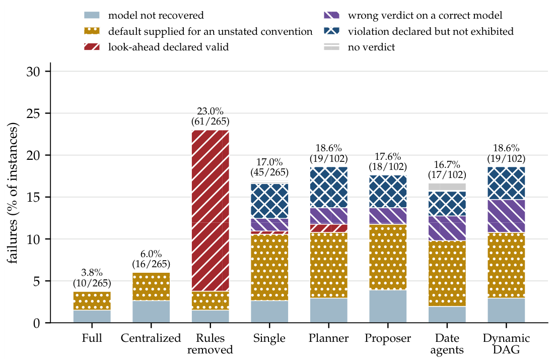
Figure A2.
The two mechanisms under a change of language model. The gain from the information rules (full method against the variant without them) lies between and points on all five models; the gain from staged recovery of conventions (full method against the centralized variant) ranges from 19.8 points to none. † Different prompts; not paired with the other models.
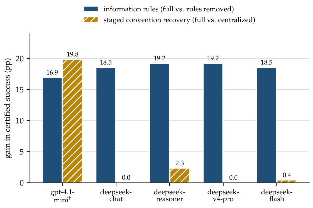
Table A6.
Cost per instance at the prose level, deepseek-reasoner: mean (standard deviation), median [interquartile range] for language-model tokens, mean (standard deviation) for requests, and median [interquartile range] for bytes exchanged between components or agents. The variant without information rules shares the full method’s language-model requests. The centralized variant and direct text to proof exchange no messages.
References
- Bailey, D. H., Borwein, J. M., López de Prado, M., & Zhu, Q. J. (2014). Pseudo-mathematics and financial charlatanism: The effects of backtest overfitting on out-of-sample performance. Notices of the American Mathematical Society, 61(5), 458–471. [Google Scholar] [CrossRef] [Scilit]
- Boldo, S., Lelay, C., & Melquiond, G. (2016). Formalization of real analysis: A survey of proof assistants and libraries. Mathematical Structures in Computer Science, 26(7), 1196–1233. [Google Scholar] [CrossRef] [Scilit]
- Cox, J. C., Ross, S. A., & Rubinstein, M. (1979). Option pricing: A simplified approach. Journal of Financial Economics, 7(3), 229–263. [Google Scholar] [CrossRef] [Scilit]
- Delbaen, F., & Schachermayer, W. (1994). A general version of the fundamental theorem of asset pricing. Mathematische Annalen, 300(1), 463–520. [Google Scholar] [CrossRef] [Scilit]
- de Moura, L., & Ullrich, S. (2021). The Lean 4 theorem prover and programming language. In Automated deduction—CADE-28 (Vol. 12699, pp. 625–635). Springer. [Google Scholar] [CrossRef] [Scilit]
- First, E., Rabe, M. N., Ringer, T., & Brun, Y. (2023, December 3–9). Baldur: Whole-proof generation and repair with large language models. 31st ACM Joint European Software Engineering Conference and Symposium on the Foundations of Software Engineering (ESEC/FSE) (pp. 1229–1241), San Francisco, CA, USA. [Google Scholar] [CrossRef] [Scilit]
- Föllmer, H., & Schied, A. (2016). Stochastic finance: An introduction in discrete time (4th ed.). De Gruyter. [Google Scholar] [CrossRef] [Scilit]
- Harrison, J. M., & Kreps, D. M. (1979). Martingales and arbitrage in multiperiod securities markets. Journal of Economic Theory, 20(3), 381–408. [Google Scholar] [CrossRef] [Scilit]
- Harrison, J. M., & Pliska, S. R. (1981). Martingales and stochastic integrals in the theory of continuous trading. Stochastic Processes and their Applications, 11(3), 215–260. [Google Scholar] [CrossRef] [Scilit]
- Harvey, C. R., Liu, Y., & Zhu, H. (2016). … and the cross-section of expected returns. Review of Financial Studies, 29(1), 5–68. [Google Scholar] [CrossRef] [Scilit]
- Jiang, A. Q., Welleck, S., Zhou, J. P., Li, W., Liu, J., Jamnik, M., Lacroix, T., Wu, Y., & Lample, G. (2023, May 1–5). Draft, sketch, and prove: Guiding formal theorem provers with informal proofs. 11th International Conference on Learning Representations (ICLR), Kigali, Rwanda. Available online: https://openreview.net/forum?id=SMa9EAovKMC (accessed on 21 August 2026).
- Li, Y., Wang, S., Ding, H., & Chen, H. (2023, November 27–29). Large language models in finance: A survey. 4th ACM International Conference on AI in Finance (ICAIF) (pp. 374–382), New York, NY, USA. [Google Scholar] [CrossRef] [Scilit]
- López de Prado, M. (2018). Advances in financial machine learning. Wiley. Available online: https://www.wiley.com/en-us/Advances+in+Financial+Machine+Learning-p-9781119482086 (accessed on 21 August 2026).
- Neveu, J. (1975). Discrete-Parameter martingales. In North-Holland mathematical library (Vol. 10). North-Holland. Available online: https://www.sciencedirect.com/bookseries/north-holland-mathematical-library/vol/10/suppl/C (accessed on 21 August 2026).
- Peskir, G., & Shiryaev, A. (2006). Optimal stopping and free-boundary problems. In Lectures in mathematics. ETH Zürich. Birkhäuser. [Google Scholar] [CrossRef] [Scilit]
- Polu, S., & Sutskever, I. (2020). Generative language modeling for automated theorem proving. arXiv, arXiv:2009.03393. [Google Scholar] [CrossRef] [Scilit]
- Snell, J. L. (1952). Applications of martingale system theorems. Transactions of the American Mathematical Society, 73(2), 293–312. [Google Scholar] [CrossRef]
- The Mathlib Community. (2020, January 20–21). The Lean mathematical library. 9th ACM SIGPLAN International Conference on Certified Programs and Proofs (CPP) (pp. 367–381), New Orleans, LA, USA. [Google Scholar] [CrossRef] [Scilit]
- Trinh, T. H., Wu, Y., Le, Q. V., He, H., & Luong, T. (2024). Solving olympiad geometry without human demonstrations. Nature, 625(7995), 476–482. [Google Scholar] [CrossRef] [Scilit]
- Wu, S., Irsoy, O., Lu, S., Dabravolski, V., Dredze, M., Gehrmann, S., Kambadur, P., Rosenberg, D., & Mann, G. (2023). BloombergGPT: A large language model for finance. arXiv, arXiv:2303.17564. [Google Scholar] [CrossRef] [Scilit]
- Wu, Y., Jiang, A. Q., Li, W., Rabe, M. N., Staats, C., Jamnik, M., & Szegedy, C. (2022). Autoformalization with large language models. In Advances in neural information processing systems 35 (NeurIPS) (pp. 32353–32368). Curran Associates, Inc. [Google Scholar] [CrossRef] [Scilit]
- Yang, K., Swope, A. M., Gu, A., Chalamala, R., Song, P., Yu, S., Godil, S., Prenger, R., & Anandkumar, A. (2023). LeanDojo: Theorem proving with retrieval-augmented language models. In Advances in neural information processing systems 36 (NeurIPS), datasets and benchmarks track (pp. 21573–21612). Curran Associates, Inc. [Google Scholar] [CrossRef] [Scilit]
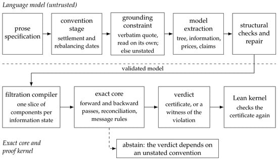
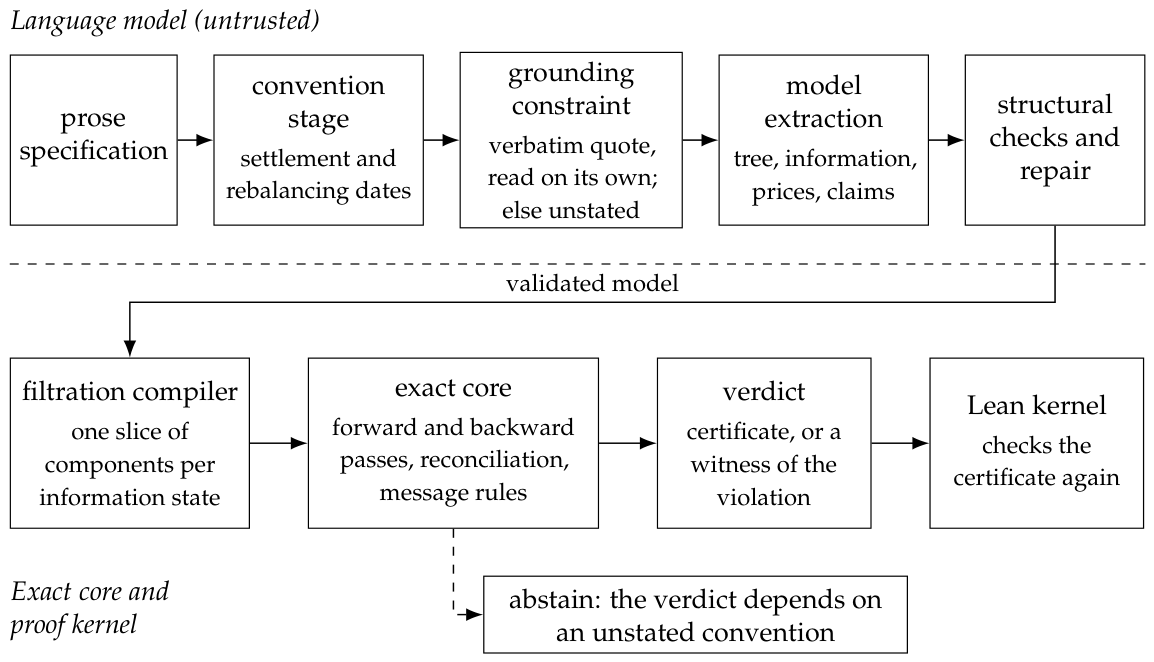
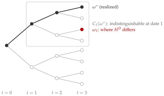
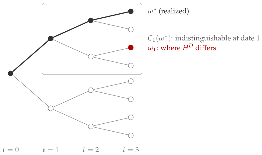
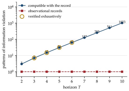
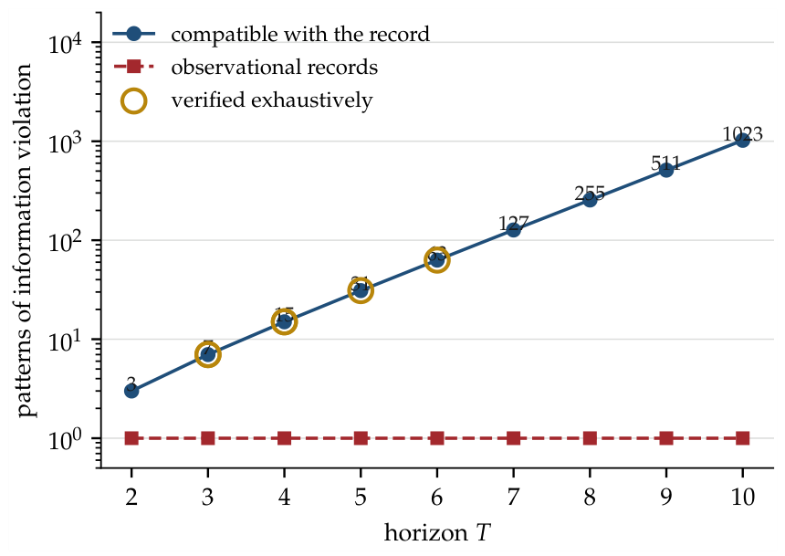
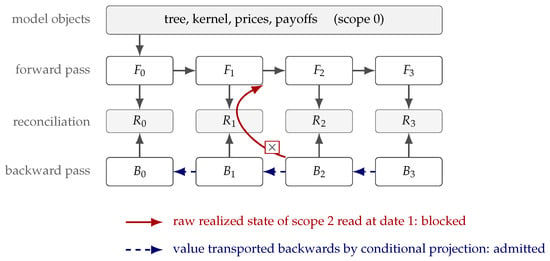
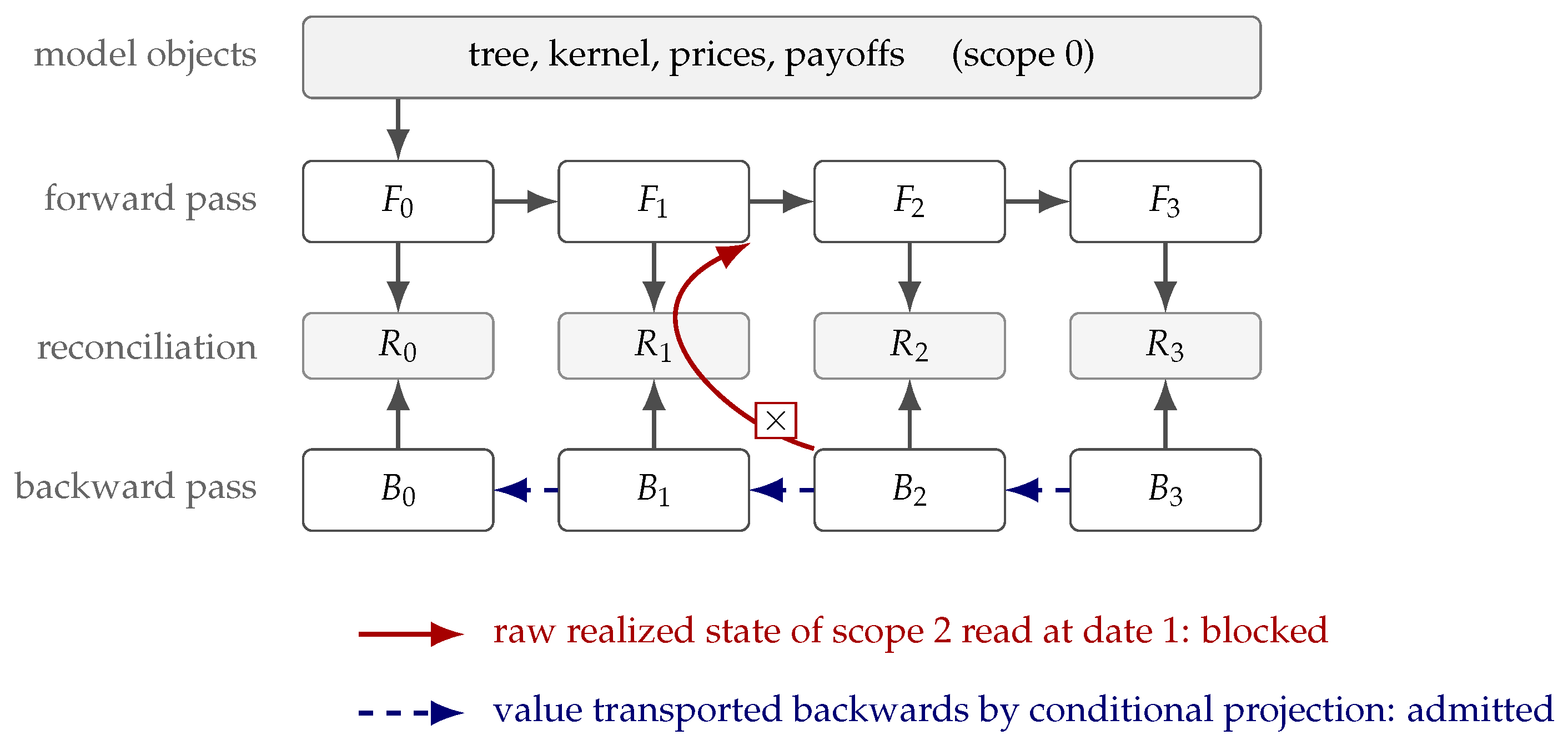
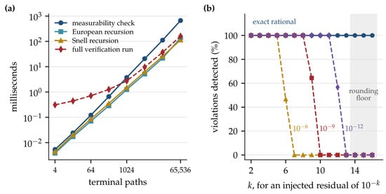
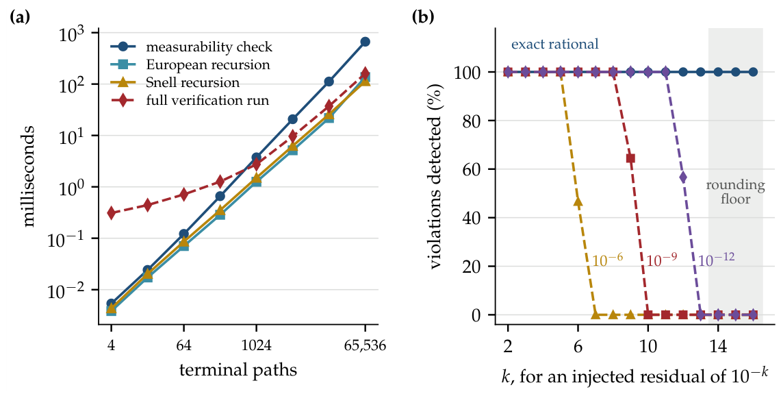
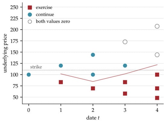
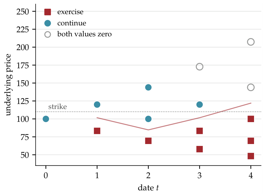

Disclaimer/Publisher’s Note: The statements, opinions and data contained in all publications are solely those of the individual author(s) and contributor(s) and not of MDPI and/or the editor(s). MDPI and/or the editor(s) disclaim responsibility for any injury to people or property resulting from any ideas, methods, instructions or products referred to in the content. |
© 2026 by the authors. Licensee MDPI, Basel, Switzerland. This article is an open access article distributed under the terms and conditions of the Creative Commons Attribution (CC BY) license.