When the Event Zero Is Wrong: Anchor Misplacement, Peak Leverage, and Spurious Amplification in Liquidation Event Studies

Abstract

Event studies of liquidation cascades locate their event zero using a rule applied to the data, usually its peak day and hour. On two Hyperliquid cascades, a zero-transaction-hash heuristic, which in fact tags time-weighted average price (TWAP) executions, feeds that rule and places the zero five hours late in one event and a day early in the other. In the mislocated windows, a two-way fixed-effects liquidation × event interaction is +1.44 and +0.48, both significant under Driscoll–Kraay errors; correctly located, on the same rows, it is a null and a negative estimate resting on one coin-minute. Because the coefficient is a difference of slopes, the peak hour, carrying 78–93% of the window’s liquidations at a low slope, pulls down whichever side contains it: every placebo window containing the peak returns a negative interaction and most excluding it a positive one. These counts are nested views of two price paths, not independent evidence. Rebuilt panels, a high–low spread proxy, and a wild cluster bootstrap over nine coins preserve the sign pattern but not every significance level. The event zero must therefore be verified against a native label before estimation; window sweeps and peak deletion do not substitute for that check.

1. Introduction

The event study design assumes that the researcher knows when the event happened. In the classical corporate finance setting, this is a mild assumption: announcements carry timestamps, and the literature on event date uncertainty (Ball & Torous, 1988; Dyckman et al., 1984) treats residual imprecision as a nuisance that widens the window rather than a threat to the sign of the estimate. In high-frequency and on-chain markets, the assumption fails in a specific way. The event of interest—a liquidation cascade, a flash crash, a de-pegging—has no announcement. Its zero is located, typically by a rule of the form “the day on which the studied quantity peaked, and the hour within that day at which it peaked.” The event zero is therefore a function of the data. In particular, it is a function of the same measured quantity whose effect the study then estimates.

The question matters because the markets in which the assumption fails are the ones in which forced selling is studied most intensively. Cryptocurrency perpetual futures venues liquidate leveraged positions automatically, and cascades of such liquidations have become the canonical stress event of the asset class. The exchange-level mechanics of liquidation and insurance funds have been documented for centralized derivatives venues (Soska et al., 2021), the incentives and instabilities of forced liquidation for lending protocols (Qin et al., 2021), and the cross-venue structure within which these events propagate (Makarov & Schoar, 2020). Studies of what a cascade does to market quality must measure liquidity from trade data because order book snapshots are rarely archived. The Roll (1984) estimator and its high–low successors (Corwin & Schultz, 2012; Abdi & Ranaldo, 2017) are the standard tools, and their reliability for cryptocurrency markets has been assessed by Dyhrberg et al. (2018) and Brauneis et al. (2021). What that literature inherits from the event study tradition is a design—an event window compared against a control period—without the one input the tradition could take for granted: a dated event.

The event study literature has long recognized that event dates can be uncertain and that window choice matters. Ball and Torous (1988) and Dyckman et al. (1984) treat date uncertainty as a source of attenuation that is addressed by widening the window. Brown and Warner (1985), Boehmer et al. (1991), MacKinlay (1997), and Kothari and Warner (2007) establish how window length and event-induced variance affect inference. Kolari and Pynnönen (2010) show that cross-sectional correlation inflates test statistics when events cluster in time. In every one of these settings, the date is known up to a small error, and the error is independent of the outcome. A different strand asks what happens when the date is chosen from the data. A zero located at the sample peak of a series is a break date estimated from that series, and the distribution theory for tests at data-selected break points (Andrews, 1993; Andrews & Ploberger, 1994; Hansen, 2000) explains why such a zero cannot be treated as a fixed regressor. Ahern (2009) shows that non-random selection of events biases event study estimates when the selection is based on the outcome. Closer still are the literatures on mismeasured assignment. Pei and Shen (2017) analyze regression discontinuity designs in which the running variable is measured with error and Battistin and Chesher (2014) the neighboring case of error in a conditioning covariate. Baker et al. (2022) document how sensitive two-way fixed-effects estimates are to when treatment is dated across units. The trade classification literature (Lee & Ready, 1991) is the structural analogue on the data side: a heuristic rule labels individual records, and its error rate propagates into every downstream estimate.

None of these literatures covers the case this paper documents. In the on-chain setting the event of interest—a liquidation cascade, a flash crash, a de-pegging, an oracle failure—has no announcement, so its zero is not merely uncertain but located by a rule applied to a series that is itself derived from the same fill record the study then analyzes. If the label that identifies that series is wrong, the error does not widen the window; it moves it. And, because the interaction coefficient of the standard design is a difference between two slopes, a window that misses a concentrated shock does not merely attenuate the estimate. The literature on mismeasured timing predicts attenuation; the literature on data-chosen break dates predicts an inflated statistic at a correctly located break. Neither predicts what we find: a large, highly significant estimate of the wrong sign at a wrongly located zero produced by assigning the hour that carries the shock to the control group.

This paper documents that failure on two Hyperliquid cascades and then asks the more general question it raises: what does an interaction design return when the treated window misses a shock that is concentrated in a single hour? Hyperliquid is a decentralized perpetual futures exchange whose complete fill record is public and carries a native liquidation field on every forced fill. In an earlier version of this research, the author identified liquidations instead by a zero transaction hash; that convention turns out to tag the protocol’s own TWAP sub-order executions, a series with no relation to liquidations and, as we show, with no cascade signature at all. We apply one fixed anchor rule—platform-wide peak day, then intraday peak hour, then a 24 h forward window—to both labels and estimate one fixed two-way fixed-effects specification of the log bid–ask spread on standardized liquidation volume and its interaction with the event dummy. Three findings follow. First, the same rule fed by the zero-hash label places the event zero five hours late in November 2025 and a full day early in January 2026. The reason is that the zero-hash daily series has no peak to pick: its peak day exceeds its runner-up by 4% in both events against 82% and 77% under the native label. With the native series as the regressor, the interaction under the heuristic anchors is +1.44 and +0.48 (both p < 0.001); under the authoritative anchors, on the same rows, it is −0.04 (p = 0.59) and −0.33 (p = 0.008). We call this the hybrid design—window from one source, regressor from another—because it is the realistic failure: a study using the zero-hash label throughout would find nothing at all. Second, the estimate moves with where the peak falls, not with the label. The coefficient β₂ is the difference between the treated and control period slopes; the authoritative peak hour carries 78% and 93% of the correctly anchored window’s liquidations and has a low slope of its own, so it pulls down whichever side of the split contains it. A placebo sliding the window across each panel returns a negative β₂ at every peak-including anchor (48 of 48 on a one-hour grid) and a significantly positive one at 73% and 60% of peak-excluding anchors. The 7 out of 120 peak-excluding exceptions on the three-hour grid are all insignificant. Third, the two events differ in what supplies the magnitude: deleting the peak hour destroys the spurious positive in one event and not in the other, so we report the sign regularity as a finding and claim no single mechanism for the size of the estimate.

The contribution is methodological and diagnostic; the paper takes no position on whether liquidations widen or narrow spreads in general. Three checks that bear on the credibility of the panels and the inference are reported alongside the results. Both nine-coin panels were rebuilt from the raw fill stream and reconciled with the archived panels. The anchor contrast was re-estimated under two alternative trade-based spread proxies that remain defined where the Roll estimator does not. And, the inference on nine coin clusters was re-examined with a wild cluster bootstrap. Section 2 describes the setting, its governance, and the two labels; Section 3 the data and the anchor rule; Section 4 the specification, its coefficients, and the inference. Section 5 reports the results, Section 6 discusses what they imply and what they cannot show, and Section 7 concludes.

2. Institutional Background

2.1. Liquidations on Hyperliquid

Hyperliquid is an order book perpetual futures exchange on its own layer-1 chain. Every fill is recorded in the public node_fills stream with the coin, price, size, side, a trade identifier (tid), a transaction hash, and—on forced fills—a liquidation object naming the liquidated account (liquidatedUser), the mark price, and the method. Forced fills reach the book through three channels: market liquidation against resting orders (method = market), absorption by the protocol’s backstop vault (method = backstop), and auto-deleveraging (ADL), in which profitable counterparties are closed against the underwater position (fill direction Auto-Deleveraging). This is the on-chain analogue of the liquidation and insurance fund mechanics studied for centralized derivatives venues (Soska et al., 2021) and lending protocols (Qin et al., 2021); Makarov and Schoar (2020) describe the cross-venue structure in which these venues sit.

Because a fill is recorded from both sides, a liquidation event is identified by pairing the records sharing a tid and counting notional once. For market and backstop liquidations, only the liquidated side carries the liquidation object, so counting records already counts events; for ADL fills, both sides carry the Auto-Deleveraging direction, so a record-level count doubles ADL notional. The event-level de-duplication used throughout corrects that; Appendix C shows that it does not bind here, where the nine-coin panels contain no ADL fills.

2.2. Governance and Regulatory Status

Hyperliquid runs as a proof-of-stake layer-1 chain whose HyperBFT consensus is operated by a stake-weighted validator set: a validator must self-delegate 10,000 HYPE, the native token, to become active, and any group of validators holding more than two-thirds of the stake forms a quorum (Hyperliquid, 2026b). On-chain authority over the exchange—the listing and delisting of markets, parameter changes, the jailing of unresponsive peers—rests with that validator set rather than an external supervisor; the Hyper Foundation operates a delegation program that conditions its support on identity verification and residence outside of restricted jurisdictions (Hyperliquid, 2026a). The reach of that authority was demonstrated on 26 March 2025 when, after manipulation of the JELLY perpetual threatened the protocol’s backstop vault, the validators voted to delist the contract and settled all open positions at USD 0.0095 (Hyperliquid, 2025a; The Block, 2025). We are not aware of any financial regulator that licenses the venue; a registration statement filed with the U.S. Securities and Exchange Commission for an exchange-traded fund holding its token states that its perpetual contracts might not legally be offered, sold, or traded by most U.S. persons (Grayscale Investments, 2026). For this paper, the relevant consequence is that the liquidation field we treat as authoritative is a protocol record written by the validators’ own execution engine and not subject to external audit. Its credibility derives from the public ledger, which anyone can replay, not regulatory oversight. The label error we document is an error in a researcher’s reading of that ledger, not in the ledger itself.

2.3. Two Labels for the Same Word

The authoritative label is the native liquidation field. The second label treats a fill as a liquidation if its transaction hash is the zero hash (0x000…0). We do not claim that this convention is in general use; we can document that it was the author’s own identification rule in an earlier version of this research, archived as the v1 replication package, and the present paper is in part a correction of that error. Hyperliquid’s application programming interface (API) documentation states that “TWAP fills have a hash of 0” (Hyperliquid, 2025b); these are the protocol’s scheduled slices of large orders, executed every thirty seconds, which have no independent on-chain transaction. Cross-tabulating the two labels on the fill record of the October 2025 cascade, the companion identification paper (Luo, 2026) finds the zero-hash set and the native liquidation set to be disjoint. A “liquidation volume” series built from the zero-hash label is therefore a TWAP execution series. This paper takes that identification as an input; nothing below depends on it beyond the fact, shown directly in Table 1, that the two series have different daily and intraday profiles.

Table 1. Platform-wide daily notional (USD million) under the two labels, event-level de-duplicated by tid. Bold marks the peak day selected by step 1 of the anchor rule under each label.

November 2025	Native Tag	Zero-Hash Tag	January–February 2026	Native Tag	Zero-Hash Tag
17 November	380.5	329.7	26 January	193.2	160.5
18 November	138.4	304.2	27 January	108.7	216.1
19 November	215.3	272.6	28 January	57.1	292.8
20 November	183.8	251.2	29 January	286.6	345.5
21 November	691.6	343.1	30 January	608.1	357.6
22 November	29.9	200.9	31 January	1075.7	300.2
23 November	24.4	159.5	1 February	104.8	202.9
24 November	104.9	197.6	2 February	139.4	241.7
25 November	95.1	177.3	3 February	135.1	314.6

Source: replication package, tableF0_platform_daily_native_D7_*.csv, and tableF0_platform_daily_zerohash_*.csv, both produced by the same parser from the public node_fills stream (Section 3.2).

2.4. Why the Anchor Rule Is Exposed

A peak-day, peak-hour rule is a function of the label, and the two series it can be fed look nothing alike. Table 1 reports platform-wide daily totals under both labels for the nine days around each event.

The native series has a cascade in it: the peak day carries 1.8 times the runner-up in both events and 20–30 times the quietest day. The zero-hash series does not. It moves between USD 160 M and USD 358 M on every one of the eighteen days, and its peak day exceeds its runner-up by 4% in both events (343.1 versus 329.7; 357.6 versus 345.5). In January, its largest single hour (USD 71.6 M at 17:00 Coordinated Universal Time (UTC) on 29 January) does not even fall on its peak day. Applying a peak-picking rule to this series selects the highest point on a line with no peak. In November, the labels agree on the day and disagree on the hour; in January, they disagree on the day, the zero-hash label ranking 30 January narrowly above 29 January, both below the true peak day of 31 January. Given the rule, the zero a researcher obtains is a deterministic function of which label is fed to it.

3. Data, Panel Construction, and the Anchor Rule

3.1. Sample

We use minute-level panels for nine perpetual contracts—BTC, ETH, SOL, XRP, BNB, DOGE, AVAX, LINK, and HYPE—over a nine-day window around each of three Hyperliquid liquidation events:

• Main event, 10 October 2025 (panel 7–15 October). The event zero is set at 21:00 UTC on 10 October, the announcement time of the macro shock that triggered the cascade, which coincides with the start of the liquidation surge. This event is a contextual baseline against which the two replication events are read; its anchor is not data-located, and it plays no role in the anchor contrast.
• Event 1, 21 November 2025 (panel 17–25 November).
• Event 2, 30–31 January 2026 (panel 26 January–3 February; the first minute in the archived panel is 23:59 UTC on 25 January).

3.2. Panel Construction and Balance

For the main event, the spread is the quoted bid–ask spread from full-depth (level 2, L2) order book snapshots. For the two replication events, no order book snapshots were collected, and the spread is the Roll (1984) estimator computed within each coin-minute from the sequence of fill prices, as is common when only trade data are available for cryptocurrency markets (Dyhrberg et al., 2018; Brauneis et al., 2021). The following details are needed to rebuild the panels from the public stream and are implemented in the panel construction script shipped with the replication package.

(a) Fills. Every record in node_fills for the nine coins is processed once per tid; the de-duplicated set therefore includes ordinary fills, TWAP sub-order fills and liquidation fills. Volume per coin-minute is the sum of price × size over these fills. (b) Last price is the price of the last fill processed within the minute, in file order; the extended panels described in Section 4.4 also record the first, highest, and lowest fill price of the minute. (c) Return is the percentage change in last price between consecutive observed coin-minutes, not consecutive clock minutes; the first observed minute per coin has no return. (d) Roll spread. Let $p_1,\dots ,p_n$ be the fill prices of a coin-minute in file order and $\mathsf{\Delta }{p}_k=p_k-p_{k-1}$. With $n\ge 4$ fills, the estimator is

$${\widehat{s}}_{it}^{\mathrm{R}\mathrm{o}\mathrm{l}\mathrm{l}}=2\sqrt{-c_{it}},\hspace{1em}\hspace{1em}{c}_{it}=\widehat{\mathrm{C}\mathrm{o}\mathrm{v}}(\mathsf{\Delta }{p}_k,\mathsf{\Delta }{p}_{k-1}),$$

(1)

where the covariance uses the $n-1$ denominator; when $c_{it}\ge 0$, the estimator has no real solution and the minute’s spread is recorded as missing, and with exactly three fills the single available pair also yields a missing value. The spread is expressed in basis points of last price, and the regression uses its logarithm. (d′) Alternative spread proxies. Because (1) is undefined whenever consecutive price changes are positively correlated, Section 5.4 re-estimates the anchor contrast under two trade-based proxies that remain defined in that region. The first is the close–high–low (CHL) estimator of Abdi and Ranaldo (2017), which for consecutive observed minutes $t$ and $t+1$ of the same coin uses the log high $h$, log low $l$, and log last price $k$,

$${\widehat{s}}_{it}^{\mathrm{C}\mathrm{H}\mathrm{L}}=\sqrt{4 (k_{it}-{\eta }_{it})(k_{it}-{\eta }_{i,t+1})},\hspace{1em}\hspace{1em}{\eta }_{it}=1/2(h_{it}+l_{it}),$$

(2)

defined only when the product under the root is positive and recorded as missing otherwise (Abdi and Ranaldo set such values to zero; a zero spread has no logarithm). The second is the within-minute high–low range in basis points of the last price,

$${\widehat{s}}_{it}^{\mathrm{H}\mathrm{L}}={10}^4 {\displaystyle \frac{P_{it}^{\mathrm{m}\mathrm{a}\mathrm{x}}-P_{it}^{\mathrm{m}\mathrm{i}\mathrm{n}}}{P_{it}^{\mathrm{l}\mathrm{a}\mathrm{s}\mathrm{t}}}},$$

(3)

which is a transaction cost proxy rather than a spread estimator in the strict sense but is defined whenever the minute contains two distinct prices. (e) Liquidation volume per coin-minute is the sum of event-level de-duplicated native tag notional, with channel attribution to market, backstop, or ADL as defined in Section 2.1. (f) Platform-wide totals used by the anchor rule count every listed perpetual, victim-side records plus ADL-paired records, de-duplicated by tid; the zero-hash platform tables in Table 1 apply the same tid de-duplication to zero-hash records. (g) TWAP volume per coin-minute, used in Section 5.1, is the sum of notional over zero-hash fills among the de-duplicated set.

Balance. The panels are unbalanced and the estimation samples much more so; Appendix B Table A4 reports the structure. A coin-minute exists only if that coin traded in that minute, so the panels hold 115,413 and 114,783 rows against 116,640 and 116,649 if every coin traded every clock minute of the span. Only one and three clock minutes, respectively, have no fill in any of the nine coins. The binding attrition is the spread rule of (d): in the estimation samples of 49,397 and 55,741 rows, the median minute contributes four coins, and only 13 of 12,857 and 26 of 12,914 min contribute all nine. With minute fixed effects, β₂ is therefore identified from cross-sectional comparisons among a handful of coins in each minute, which is a source of noise we do not model. It does not threaten the anchor contrast, which within each event uses exactly the same available rows under both anchors. Appendix B Table A5 shows that the contrast survives two changes aimed at this structure: dropping the minute fixed effects (coin fixed effects and a main effect of D only) and restricting the sample to minutes in which at least six coins are observed. Under both, the heuristic anchor estimates remain positive and significant and the authoritative anchor estimates remain a null (Event 1) and negative (Event 2, where they become stronger).

3.3. The Anchor Rule and Its Own Degrees of Freedom

For the two replication events, the event zero is located by a two-step rule applied to platform-wide totals: first, the calendar day (UTC) with the largest notional within the nine-day window; second, within that day, the clock hour with the largest notional. The event zero is the start of that hour, and the event window is the 24 h [zero, zero + 24 h). The rule is applied once with each label, and both applications are computed in code from the tables in the replication package rather than fixed as constants. We refer to the zero located with the native label as the authoritative anchor and to the zero located with the zero-hash label as the heuristic anchor. Table 2 reports both applications.

Table 2. The two-step anchor rule applied to platform-wide totals under each label.

	Event 1 (November 2025)	Event 2 (January 2026)
Native tag: peak day (USD M)	21 November (691.6)	31 January (1075.7)
Native tag: runner-up day (USD M)	17 November (380.5)	30 January (608.1)
Native tag: peak/runner-up	1.82	1.77
Native tag: peak hour within peak day (USD M)	21 November 2025, 07:00 UTC (497.6)	31 January 2026, 18:00 UTC (694.7)
Native tag: event zero by the rule	21 November 2025, 07:00 UTC	31 January 2026, 18:00 UTC
Zero-hash tag: peak day (USD M)	21 November (343.1)	30 January (357.6)
Zero-hash tag: runner-up day (USD M)	17 November (329.7)	29 January (345.5)
Zero-hash tag: peak/runner-up	1.04	1.04
Zero-hash tag: peak hour within peak day (USD M)	21 November 2025, 12:00 UTC (46.1)	30 January 2026, 18:00 UTC (42.6)
Zero-hash tag: event zero by the rule	21 November 2025, 12:00 UTC	30 January 2026, 18:00 UTC
Zero-hash tag: largest single hour in the nine-day window	21 November 2025, 12:00 UTC (46.1)	29 January 2026, 17:00 UTC (71.6)
Displacement of the heuristic zero from the authoritative zero	+5 h, same day	−24 h, previous day

The two displacements have different geometries and are reported separately throughout. In Event 1, the two 24 h windows overlap by 1140 out of 1440 min (79.2%); in Event 2, they do not overlap at all—the heuristic window ends at the minute the authoritative window begins.

The rule carries choices we inherit and hold fixed: peak day before peak hour rather than a global peak hour, a forward rather than a centered window, and 24 h rather than another length. The first is not innocuous. Under the zero-hash label, the largest single hour of the January window falls on 29 January, not on that label’s own peak day, so a researcher using “the largest hour in the window” would have obtained a third zero, 29 January 17:00 UTC. We do not estimate that specification and make no claim about what it would return; we report it to make explicit that our results are conditional on the two-step rule and are not a statement about peak-picking rules in general.

3.4. Standardization, the Event Dummy, and the Hybrid Design

Let $L_{it}$ be the liquidation notional of coin $i$ in minute $t$ and ${\sigma }_L$ the sample standard deviation of $L_{it}$ over the non-zero coin-minutes of the event panel. The regressor is

$${\mathrm{l}\mathrm{i}\mathrm{q}}_{it}=L_{it}/{\sigma }_L,\hspace{1em}\hspace{1em}{D}_t=\mathbf{1}\{t_0\le t<t_0+24 \mathrm{h}\},$$

(4)

so that coefficients read as the spread response per standard deviation of liquidation volume; zero-liquidation minutes take the value zero. The event dummy $D_t$ equals one for the 24 h from the event zero $t_0$, and the interaction term is ${\mathrm{l}\mathrm{i}\mathrm{q}}_{it}\times D_t$.

One design choice needs to be stated plainly. In the anchor contrast of Section 5.1, the regressor is the native tag liquidation series under both anchors; only the window moves. This is a hybrid: the window comes from the heuristic label, the intensity from the authoritative one. It is the relevant counterfactual for a study that takes its event dates from an external source—a dashboard, a news timeline, a prior paper—and its regressor from the exchange’s own data, and it is the configuration under which the earlier version of this research reported its results. The other configuration, in which the zero-hash label supplies both the window and the regressor, is reported alongside it in Section 5.1 and Appendix C Table A10.

4. Empirical Design

4.1. Specification

All estimates use the same two-way fixed-effects specification,

$$\mathrm{l}\mathrm{o}\mathrm{g} s_{it}={\beta }_1 {\mathrm{l}\mathrm{i}\mathrm{q}}_{it}+{\beta }_2 ({\mathrm{l}\mathrm{i}\mathrm{q}}_{it}\times D_t)+{\beta }_3 r_{it}+{\beta }_4\mathrm{l}\mathrm{o}\mathrm{g} v_{it}+{\mu }_i+{\lambda }_t+{\epsilon }_{it},$$

(5)

where $i$ indexes coins and $t$ minutes, $s_{it}$ is the spread of (1) in basis points, ${\mathrm{l}\mathrm{i}\mathrm{q}}_{it}$ and $D_t$ are defined in (4), $r_{it}$ is the return and $v_{it}$ the dollar volume of the coin-minute, and ${\mu }_i$ and ${\lambda }_t$ are coin and minute fixed effects. The minute fixed effects absorb the main effect of $D_t$ and every other common time-varying factor, so ${\beta }_2$ is identified from the cross-coin covariation of liquidation volume and spreads within event minutes relative to non-event minutes. The control coefficients ${\beta }_3$ and ${\beta }_4$ are reported with the main estimates in Table 3. The return coefficient is small and insignificant, the log-volume coefficient is negative and precisely estimated in all four specifications of Table 3, and neither moves when the anchor moves, as expected of controls that do not interact with the window.

Table 3. Same specification, same rows, same regressor, two anchors.

Event	Anchor	β1 (se)	β2 (se)	β3 (se)	β4 (se)	p (β2), DK	β1 + β2
Event 1 (21 November 2025)	heuristic (zero-hash tag)	0.1023 *** (0.0245)	1.4372 *** (0.2947)	−1.2427 (8.1215)	−0.1264 *** (0.0082)	<0.001	1.5395
Event 1 (21 November 2025)	authoritative (native tag)	0.1326 (0.0703)	−0.0396 (0.0733)	−1.6526 (8.1080)	−0.1264 *** (0.0082)	0.5893	0.0930
Event 2 (30/31 January 2026)	heuristic (zero-hash tag)	0.0731 * (0.0297)	0.4832 *** (0.0876)	−0.6719 (5.0985)	−0.1324 *** (0.0081)	<0.001	0.5563
Event 2 (30/31 January 2026)	authoritative (native tag)	0.3784 ** (0.1255)	−0.3306 ** (0.1255)	−0.9580 (5.0771)	−0.1328 *** (0.0081)	0.0084	0.0478

Notes: Coin and minute fixed effects; Driscoll–Kraay (DK) standard errors, Bartlett kernel, bandwidth 10 (Equation (7)). N = 49,397 (Event 1) and 55,741 (Event 2); both anchors within an event use the identical estimation sample and the identical bandwidth. β₃ is the coefficient on the return and β₄ on log volume; the event zeros are those of Table 2; the t-statistics of β₂ and the ratio |β₁ + β₂|/|β₁| are reported in Section 5.4. *** p < 0.001, ** p < 0.01, * p < 0.05.

What the coefficients are. Because $D_t$ is binary, (5) fits one slope where $D_t=0$ and another where $D_t=1$. It is algebraically identical to the two-slope parameterization

$$\mathrm{l}\mathrm{o}\mathrm{g} s_{it}={\gamma }_c {\mathrm{l}\mathrm{i}\mathrm{q}}_{it}(1-D_t)+{\gamma }_t {\mathrm{l}\mathrm{i}\mathrm{q}}_{it} D_t+{\beta }_3 r_{it}+{\beta }_4\mathrm{l}\mathrm{o}\mathrm{g} v_{it}+{\mu }_i+{\lambda }_t+{\epsilon }_{it},$$

(6)

with ${\gamma }_c={\beta }_1$ the control period slope, ${\gamma }_t={\beta }_1+{\beta }_2$ the treated period slope, and ${\beta }_2={\gamma }_t-{\gamma }_c$ their difference. We state this explicitly because it governs the interpretation in Section 5.3, and we verify it by estimating (6) directly: across both events and both anchors, ${\widehat{\gamma }}_c$ equals ${\widehat{\beta }}_1$ and ${\widehat{\gamma }}_t$ equals ${\widehat{\beta }}_1+{\widehat{\beta }}_2$ to four decimal places. It follows that an observation influences ${\beta }_2$ through whichever of the two slopes its own period supplies.

4.2. Inference

Standard errors are those of Driscoll and Kraay (1998) (DK) with a Bartlett kernel and bandwidth

$$m=\lfloor T^{1/4}\rfloor =10,$$

(7)

where $T$ is the number of distinct minutes in the estimation sample (12,857 and 12,914) following the panel heteroskedasticity- and autocorrelation-consistent (HAC) tradition of Newey and West (1987) and the guidance of Petersen (2009). The Driscoll–Kraay estimator averages the moment conditions across coins within each minute and treats the resulting time series as the object of inference. Its consistency relies on $T\to \mathrm{\infty }$ and makes no demand on the number of coins. But, the estimation samples are sparse in the cross-section (the median minute contributes four out of nine coins, Appendix B Table A4) so that cross-sectional average is noisy, a feature we document rather than model. The marginal effect ${\beta }_1+{\beta }_2$ is reported with the delta method standard error for a linear combination,

$$\mathrm{s}\mathrm{e}({\widehat{\beta }}_1+{\widehat{\beta }}_2)=\sqrt{\mathrm{V}\mathrm{a}\mathrm{r}{\widehat{\beta }}_1+\mathrm{V}\mathrm{a}\mathrm{r}{\widehat{\beta }}_2+2\mathrm{C}\mathrm{o}\mathrm{v}({\widehat{\beta }}_1,{\widehat{\beta }}_2)},$$

(8)

and a normal approximation p-value; with residual degrees of freedom near 36,000 and 43,000, the $t$ and normal p-values agree to three significant figures. We also report the ratio $|{\beta }_1+{\beta }_2|/|{\beta }_1|$ and call one minus that ratio the neutralization share only where ${\beta }_2$ is significant. Within-$R^2$ is not reported because its definition under two-way fixed effects in the estimation library does not correspond to the usual one-way quantity.

Two comparators are reported alongside these (Section 5.4 and Appendix A Table A1). The first is clustering by coin and by coin and minute. The cluster counts are nine coins and 12,857 or 12,914 min. Nine clusters in the coin dimension is far below the range in which cluster-robust inference is reliable (Cameron et al., 2008; Cameron & Miller, 2015), so the two-way clustered and coin-clustered statistics are reported for completeness and are not given independent weight. The second takes the coin dimension seriously by other means, a restricted wild cluster bootstrap (WCB) over coins (Cameron et al., 2008). Writing $\tilde{X}$ for the regressors of (5) after the two-way within transformation, $\tilde{\beta }$ for the estimate under the null ${\beta }_2=0$ and $\tilde{u}$ for its residuals, each bootstrap sample is

$$y_{it}^{\ast }={\tilde{X}}_{it}\tilde{\beta }+{\tilde{u}}_{it} w_{g(i)},\hspace{1em}\hspace{1em}{t}^{\ast }={\widehat{\beta }}_2^{\ast }/{\mathrm{s}\mathrm{e}}_{\mathrm{c}\mathrm{o}\mathrm{i}\mathrm{n}}({\widehat{\beta }}_2^{\ast }),\hspace{1em}\hspace{1em}{p}^{\ast }={\displaystyle \frac{1}{B}}{\displaystyle {\sum }_{b=1}^B}\mathbf{1}\{|t_b^{\ast }|\ge |\widehat{t}|\},$$

(9)

where $w_g$ is drawn independently for each coin $g$ from the six-point distribution of Webb, which MacKinnon and Webb (2018) recommend for few clusters because the Rademacher distribution has only 2⁹ = 512 distinct draws with nine clusters. Because $w_g$ varies across coins, $y^{\ast }$ is re-demeaned in both dimensions before re-estimation. The observed and bootstrap statistics use the same coin-clustered standard error, and $B=9999$. Appendix A Table A1 also reports the exact Rademacher version, which enumerates all 512 sign vectors instead of sampling. The bootstrap does not rescue an estimate that nine clusters cannot support; it reports how much of the nominal significance survives when the coin dimension is treated as the unit of dependence. The answer (Section 5.4) is not much on either side of the contrast. With nine clusters, the bootstrap p-values are 0.064 and 0.015 for the two heuristic anchor estimates, whose coin-clustered t-statistics are 4.08 and 8.22 and 0.068 for the Event 2 corrected estimate (0.019 under the exact Rademacher enumeration).

4.3. Sample Selection and the Spread Proxy

The estimation sample drops coin-minutes with an undefined Roll spread, a missing return or missing log volume; the first is binding. Appendix B Table A6 reports the selection: 57.2% and 51.4% of coin-minutes have an undefined spread, and 87% and 79% of those have at least three fills. They are undefined because the lag-one serial covariance of within-minute price changes is non-negative, the region in which the Roll estimator has no real solution (Harris, 1990), not because prices did not move. Zero-volume minutes do not occur; nine rows per panel lack a return. The anchor contrast is unaffected by the selection because both anchors within an event use the identical estimation sample ($N$ = 49,397 and 55,741). Roll-estimated spreads are not comparable in level to the main event’s quoted spreads, which limits comparison across rows of Appendix C Table A11 but not any within-event comparison.

The selection is not neutral with respect to the event, but it is not concentrated where one might expect. The Roll estimator assumes serially uncorrelated true returns and a stationary order flow, assumptions that fail inside of a cascade, where same-direction forced fills induce positive serial correlation in price changes and push $c_{it}$ above zero; one would expect the peak hour to be where the estimator fails most often. Appendix B Table A7 reports the definedness rate separately for the authoritative peak hour, the remaining 23 h of the authoritative window and the control period. The peak hour is in fact the regime in which the spread is defined most often: 51.7% and 58.0% of its coin-minutes against 43.5% and 50.7% in the rest of the window and 42.7% and 48.3% in the control period. Among coin-minutes that contain liquidations, the gap is wider still (72.1% and 85.2% in the peak hour against 50.1% and 67.3% in the control period). Defined peak-hour coin-minutes are heavily traded (a median of 197 and 234 fills against 32 and 40 for defined minutes in the panel as a whole, see Appendix B Table A6). But undefined peak-hour minutes are heavily traded, too (medians of 121 and 90), so the number of fills does not by itself decide which minutes survive, and we report the pattern without claiming a mechanism. As a consequence, 99.1% and 100% of the peak hour’s liquidation notional sit in rows with a defined spread. Where the estimator does fail in the peak hour, it fails because $c_{it}\ge 0$: 92.7% and 96.5% of the undefined peak-hour minutes have four or more fills. Those minutes carry USD 4.3 M and USD 0.03 M of liquidations. The selection therefore removes off-peak minutes from both sides of every split at similar rates: among coin-minutes that carry liquidations, 49.5% and 64.8% are defined inside of the heuristic window against 50.4% and 67.7% outside of it. Its effect on ${\beta }_2={\gamma }_t-{\gamma }_c$ is not signed by these rates. The dropped rows can move either slope, but they carry the least leverage on whichever slope contains the peak hour—the control slope under the heuristic anchor, the treated slope under the authoritative anchor. The direction depends on whether those rows carry higher or lower costs per unit of liquidation than the retained ones, which the Roll sample cannot reveal. We therefore test the selection rather than signing it. Section 5.4 re-estimates the contrast under (2) and (3), whose definedness rates by regime are reported in Appendix B Table A8 next to those of (1) and under (3) on the Roll estimation sample itself, which separates the effect of restoring the dropped rows from the effect of changing the measure. The range (3) is defined in 95.6% and 92.8% of coin-minutes in every coin-minute that carries liquidations in Event 1 and in all but 0.2% of them in Event 2 (100% of their notional in both), so it restores almost all of the dropped minutes. The close–high–low estimator (2) does not. Its two-period product is negative whenever the close lies on opposite sides of two consecutive mid-ranges, which is exactly what a one-directional move produces. It is therefore undefined in the two largest coin-minutes of Event 1’s peak hour and retains only 8.3% of that peak hour’s liquidation notional (95.8% in Event 2). It is reported because it is the standard trade-based alternative to Roll, with that caveat attached.

4.4. Panel Construction, Re-Estimation, and Verification

All specifications were re-estimated from the minute panels with the event dummies rebuilt from the stated timestamps, and every table was generated from that output. Both nine-coin panels were also rebuilt from the raw node_fills stream with the panel construction script shipped in the replication package unchanged except that its input and output paths are read from the environment. The rebuilt panels were then compared with the archived panels from which every estimate in this paper is computed (Appendix B Table A9). The two agree row by row on every input column—liquidation notional by channel, volume, fill count, last price, Roll spread, and TWAP volume—with a maximum absolute difference of zero. They also agree on the native tag platform-wide daily and hourly tables that the script writes (the input to Table 2 and to the native tag columns of Table 1; the zero-hash columns are rebuilt separately, see Section 3.2) and on the anchor contrast coefficients the script itself reports. A second parser, which shares no code with the panel builder, recomputes only the peak hour and the ten coin-minutes of Table A2 directly from the raw records. It agrees with the panels on every liquidation-carrying peak-hour coin-minute (104 and 61) and on the ten Table A2 coin-minutes to within USD 10⁻⁶ and reproduces the platform-wide peak-hour totals of Table 2. The earlier version of this research mislabeled liquidations at exactly this stage of the pipeline; the check establishes that the panels used here are what the shipped code produces from the public stream, not that the code is right, which is what the rest of the paper is about.

Use of generative AI. The Python scripts (Python 3.13 with pandas 2.3.3, NumPy 2.4.2, SciPy 1.17.1, linearmodels 7.0 and Matplotlib 3.10.8) that build and verify the minute panels, estimate every specification, and generate every table and figure reported here were written with the assistance of a generative AI tool, as was the drafting of the text. Every reported number was verified by the author against the output of the deposited scripts, and the scripts are included in the replication package so that readers can check them independently. The specification, the anchor rule, the choice of diagnostics, and every interpretation are the author’s. Details are given in the Acknowledgments.

5. Results

5.1. The Anchor Contrast

Table 3 estimates (5) for the two replication events under both anchors on the same rows and with the same native tag regressor; only the window moves. Under the authoritative anchors, the interaction is a null in Event 1 (a null, not a smaller effect) and negative in Event 2; under the heuristic anchors, it is +1.44 and +0.48 with p < 0.001, apparent amplification by factors of 15 and 7.6. The control coefficients β₃ and β₄ do not move with the anchor. Appendix C Table A11 adds, for context, the main event of October 2025, whose zero is an announcement time and whose interaction is also significantly negative; nothing in the data, correctly anchored, points to amplification, and Section 5.4 returns to how much weight the Event 2 estimate can bear.

A reader shown only the two heuristic rows would conclude that cascades sharply amplify the liquidation-to-spread channel. Those rows are the hybrid design of Section 3.4. Appendix C Table A10 completes the 2 × 2 with the zero-hash series as the regressor; it has no relationship with spreads at either anchor (β₂ insignificant in all four rows), so a study that used the zero-hash label throughout would report nothing. The dangerous configuration is the hybrid one, in which a window located by the wrong series is applied to the right one.

5.2. Window Geometry: Where the Shock Is

Table 4 and Figure 1 show where the two windows fall relative to the liquidations.

Table 4. Window geometry and liquidation activity inside of the two 24 h windows (nine-coin panel).

Quantity	Event 1 (21 November 2025)	Event 2 (30/31 January 2026)
Event zero, authoritative tag	21 November 2025, 07:00	31 January 2026, 18:00
Event zero, heuristic tag	21 November 2025, 12:00	30 January 2026, 18:00
Shift	5 h, same day	24 h, previous day
Overlap of the two 24 h windows	1140/1440 min (79.2%)	0/1440 min (0.0%)
Nine-coin peak liquidation hour (UTC)	21 November 2025, 07:00 (USD 469.3 M)	31 January 2026, 18:00 (USD 681.0 M)
Peak hour inside of the authoritative window	yes	yes
Peak hour inside of the heuristic window	no	no
Nine-coin liquidations inside of the authoritative window	USD 604.1 M	USD 733.1 M
Nine-coin liquidations inside of the heuristic window	USD 92.2 M	USD 402.2 M
Heuristic/authoritative	0.153	0.549
Peak hour share of authoritative window	77.7%	92.9%
Coin-minutes with liquidations, authoritative window	782/12,864 (6.08%)	452/12,812 (3.53%)
Coin-minutes with liquidations, heuristic window	568/12,817 (4.43%)	520/12,670 (4.10%)

Notes: Nine-coin liquidation notional is the event-level de-duplicated native tag series used in the regressions. The peak hour is the clock hour with the largest nine-coin liquidation notional in the panel; it coincides with the platform-wide peak hour in both events (Figure 1), whose dollar value is larger because it includes all listed perpetuals.

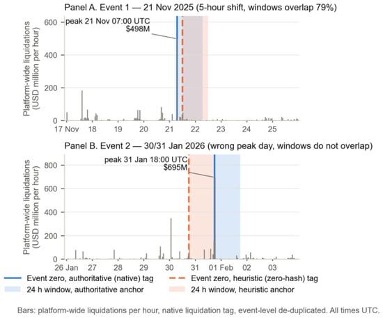
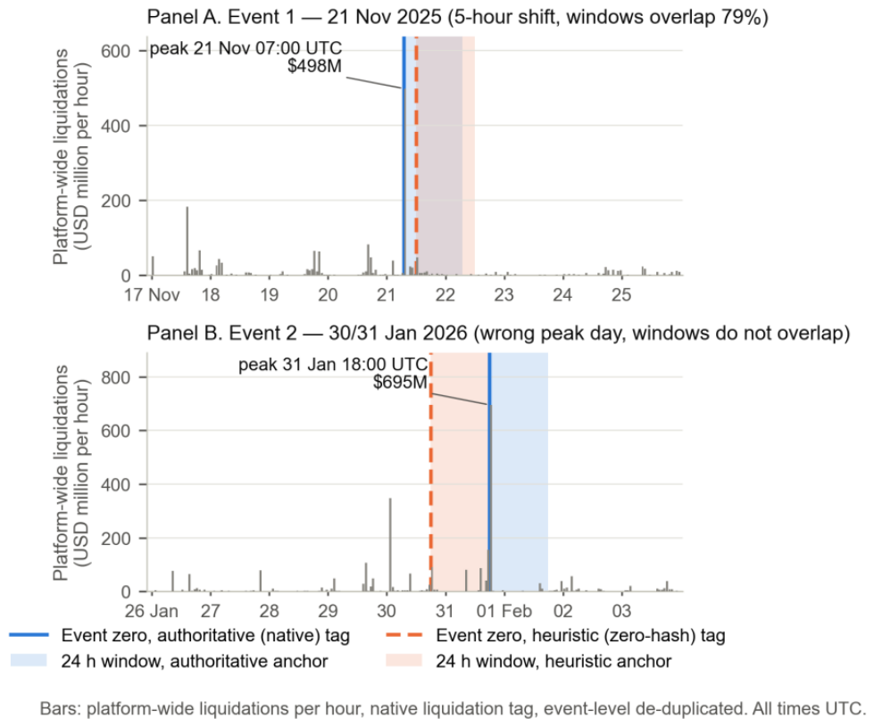
Figure 1. Platform-wide native tag liquidations per hour (USD million) and the two 24 h event windows. Panel (A): Event 1, 17–25 November 2025. Panel (B): Event 2, 26 January–3 February 2026. Solid line and blue band: authoritative anchor; dashed line, and orange band: heuristic anchor. Bars are platform-wide totals (all listed perpetuals), the input to step 2 of the anchor rule, so the annotated peak-hour values exceed the nine-coin values in Table 4. All times UTC.

In Event 1, the cascade is concentrated in a single hour: 07:00 UTC carries USD 469.3 M of the USD 604.1 M in the authoritative window. The heuristic anchor starts five hours later, so the heuristic window contains USD 92.2 M, 15% of the authoritative total, and places the hour in which the cascade happened in the comparison period. In Event 2, the heuristic label misidentifies the peak day: its window is precisely the 24 h before the authoritative zero, and the authoritative peak hour, 92.9% of its window’s total, lies just outside of it. That window is not a shifted view of the same event; it is a window on the run-up compared against a control period containing the cascade.

5.3. What β₂ Measures and What It Depends On

Section 4.1 established that β₂ is the difference between the treated period and control period slopes (Equation (6)). Table 5 decomposes it; Table 6 and Figure 2 then slide the window across each panel and Table A12 deletes the observations alleged to drive the pattern.

Table 5. The two slopes behind β₂.

Event	Treated Window	Control Period Slope β1	Treated Period Slope β1 + β2	β2 = Difference	t (β2)
1	heuristic anchor, 24 h (peak hour excluded)	0.1023	1.5395	1.4372 ***	4.88
1	authoritative anchor, 24 h (peak hour included)	0.1326	0.0930	−0.0396	−0.54
1	the authoritative peak hour alone (1 h)	0.1510	0.0808	−0.0701	−0.80
1	median over the 60 placebo anchors that exclude the peak	0.1072 (sd 0.0059)	1.2587 (sd 1.0174)	1.1543	—
1	median over the 8 placebo anchors that include the peak	0.1305	0.0945	−0.0359	—
2	heuristic anchor, 24 h (peak hour excluded)	0.0731	0.5563	0.4832 ***	5.52
2	authoritative anchor, 24 h (peak hour included)	0.3784	0.0478	−0.3306 **	−2.63
2	the authoritative peak hour alone (1 h)	0.3841	0.0466	−0.3375 **	−2.66
2	median over the 60 placebo anchors that exclude the peak	0.0817 (sd 0.0031)	0.5414 (sd 1.0944)	0.4611	—
2	median over the 8 placebo anchors that include the peak	0.3402	0.0576	−0.2825	—

Notes: Placebo anchors are the 24 h forward windows of Table 6. Italic rows are medians across anchors, not single estimates. *** p < 0.001, ** p < 0.01.

Table 6. Anchor placebo: the 24 h forward window slid across each nine-day panel in 3 h steps; same specification at every anchor.

	Event 1 (21 November 2025)	Event 2 (30/31 January 2026)
Anchors tried (24 h forward window, 3 h step)	68	68
Windows that exclude the authoritative peak hour	60	60
… share with β2 > 0 and p < 0.05	73.3%	60.0%
… share with t(β2) ≥ 4	16.7%	18.3%
… median β2	1.154	0.461
… range of β2	−0.07 to 3.85	−0.53 to 4.76
Windows that include the authoritative peak hour	8	8
… share with β2 < 0	100%	100%
… share with β2 < 0 and p < 0.05	0%	100%
… range of β2	−0.045 to −0.016	−0.331 to −0.275
Heuristic anchor: β2 (t)	1.4372 (4.88)	0.4832 (5.52)
Heuristic anchor: rank of t among peak-excluding anchors	6 of 60	3 of 60
Sign counterexamples, three-hour grid
… peak-including anchors with β2 > 0	0 of 8	0 of 8
… peak-excluding anchors with β2 < 0	5 of 60	2 of 60
… largest |t| among counterexamples; number significant at 5%	1.16; 0	0.63; 0
One-hour grid
Anchors tried (24 h forward window, 1 h step)	204	204
Peak-including anchors: β2 < 0	24 of 24	24 of 24
Peak-excluding anchors: share with β2 > 0 and p < 0.05	71.7%	57.8%
Peak-excluding anchors with β2 < 0	15 of 180	7 of 180
… largest |t| among them; number significant at 5%	1.16; 0	0.69; 0
Largest t (β2) on the one-hour grid (anchor)	6.84 (21 November 2025, 10:00)	6.53 (3 February 2026, 04:00)
Anchors whose 24 h window is truncated by the panel end (3 h/1 h grid)	3/11	3/11

Notes: Anchors run from the first full hour of each panel to 12 h before its end, so the last three anchors on the three-hour grid (eleven on the one-hour grid) have windows truncated by the panel end to 21–15 h (23–13 h on the one-hour grid). The two largest β₂ on the three-hour grid (4.75 and 4.76, t = 6.50 and 6.49) and the largest on the one-hour grid (4.76) come from these truncated windows, anchored on 3 February, and are reported as estimated. The authoritative anchor of Event 1 (07:00) does not fall on the three-hour grid and is shown separately in Figure 2; peak-including anchors are the grid points within 24 h before the peak hour. The lower block reports the explicit counterexample counts behind every statement about the sign in the text; the peak-excluding exceptions are the windows anchored on 17 November, which contain Event 1’s second-largest liquidation hour (USD 159.4 M at 14:00 UTC) and two thin windows on 30 January. The full 136-row and 408-row tables are in the replication package.

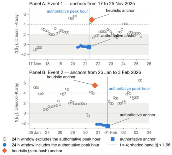
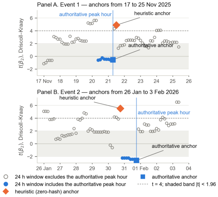
Figure 2. Anchor placebo. Each point is the Driscoll–Kraay t-statistic of β₂ for a 24 h forward window starting at the anchor time on the horizontal axis. Open gray points: windows that exclude the authoritative peak hour; filled blue points: windows that include it. Orange diamond: the heuristic anchor; blue square: the authoritative anchor (Table 3). Vertical line: the authoritative peak hour. Dashed line: t = 4; shaded band: |t| < 1.96. Panel (A): Event 1; Panel (B): Event 2.

The peak hour has a low slope of its own. Treating that single hour as the event window gives a treated period slope of 0.0808 in Event 1 and 0.0466 in Event 2 against control period slopes of 0.1510 and 0.3841. In Event 2, that one-hour specification alone returns β₂ = −0.3375 (t = −2.66), essentially the whole authoritative anchor estimate. Because the hour carries 78% and 93% of the correctly anchored window’s liquidations, it dominates whichever side of the split it falls on. The cross-anchor dispersion in Table 5 is uninformative about where the magnitude of a positive β₂ comes from. Every peak-excluding anchor leaves the peak in its control period, so a common depression of the control period slope appears across those anchors as a level, not a variance, and the small standard deviations (0.0059 and 0.0031) have no power against it. What they do show is that the treated period slope of a thin 24 h window is high and unstable (standard deviations 1.0174 and 1.0944).

If the sign of β₂ tracks peak membership, the heuristic anchor should not be special: any 24 h window excluding the peak hour should behave the same way. Table 6 and Figure 2 test this by sliding the window across each nine-day panel in three-hour steps and on a one-hour grid, re-estimating at every anchor. These estimates are nested views of one price path and one shock; they describe the estimator’s behavior are not independent evidence, and we draw no inference from counting them.

Of the 60 peak-excluding anchors in each event, 73% and 60% return a significantly positive β₂ and 17% and 18% return t ≥ 4. The median β₂ is +1.15 in Event 1, close to the heuristic anchor’s +1.44, which ranks sixth out of sixty by t; windows on days well away from either cascade produce t-statistics between 4.7 and 6.5. The relationship between peak membership and the sign is one-directional. Every anchor whose window contains the authoritative peak hour returns a negative β₂—16 out of 16 on the three-hour grid and 48 out of 48 on the one-hour grid, all insignificant in Event 1 and all significant in Event 2, the pattern of Table 3’s authoritative rows. The converse does not hold: 7 out of 120 peak-excluding anchors on the three-hour grid and 22 out of 360 on the one-hour grid also return a negative β₂, but every exception is insignificant (largest |t| = 1.16), so no significant β₂ contradicts peak membership on either grid. The heuristic anchor itself is unremarkable among peak-excluding anchors: the estimate does not depend on how the window got there.

If the peak hour is what makes the difference, deleting it should remove the pattern, and Appendix C Table A12 re-runs the placebo with the authoritative peak hour deleted and with the five largest coin-minutes deleted. The two events answer differently. In Event 2, deleting the peak hour raises the control period slope from 0.082 to 0.381, leaves the treated slope at 0.54, and collapses the spurious positive: the heuristic estimate falls from +0.48 (t = 5.5) to +0.22 (t = 1.4). In Event 1, the control slope barely moves, and the heuristic estimate stays at +1.41 (t = 4.63). What flips there is the authoritative anchor, from −0.04 to +1.03 (t = 4.05), because once the peak is gone the correctly anchored window is also just thin flow. The common element is the sign, which follows peak membership and, as it should, stops doing so once the peak is deleted. The magnitude comes from the peak depressing the control slope in Event 2 and, from the high slope, a thin 24 h window carries in Event 1 regardless, and we offer no single explanation for the latter.

5.4. Influence, Inference, and the Spread Proxy

The same concentration makes the estimate at the correct anchor a leverage result. Table 7 re-estimates the four rows of Table 3 after dropping the single largest and the five largest liquidation coin-minutes under Driscoll–Kraay and two-way clustered standard errors and with the wild cluster bootstrap p-value of (9). Appendix A Table A1 adds three further covariance estimators and the exact Rademacher bootstrap; Table A2 lists the five coin-minutes.

Table 7. Influence and inference for the four anchor contrast estimates.

Event	Anchor	Sample	N	β2	t, DK bw 10	t, Two-Way Clustered	p, Wild Cluster Bootstrap over Coins (Webb)
1	heuristic	all	49,397	1.4372	4.88 ***	3.59	0.064
1	heuristic	drop top-1	49,396	1.4010	4.70 ***	3.56	0.071
1	heuristic	drop top-5	49,393	1.1730	3.82 ***	2.85	0.069
1	authoritative	all	49,397	−0.0396	−0.54	−0.69	0.331
1	authoritative	drop top-1	49,396	0.0479	0.55	0.44	0.850
1	authoritative	drop top-5	49,393	−0.0262	−0.14	−0.13	0.892
2	heuristic	all	55,741	0.4832	5.52 ***	7.96	0.015
2	heuristic	drop top-1	55,740	0.2532	2.24 *	2.24	0.063
2	heuristic	drop top-5	55,736	0.0459	0.28	0.21	0.773
2	authoritative	all	55,741	−0.3306	−2.63 **	−1.94	0.068
2	authoritative	drop top-1	55,740	−0.1349	−1.01	−0.69	0.541
2	authoritative	drop top-5	55,736	0.4198	1.55	2.30	0.063

Notes: “Top” coin-minutes are ranked by liquidation notional within the whole nine-day panel, not within the estimation sample (Appendix A Table A2). Two-way clustering is by coin (nine clusters) and minute (12,857 and 12,914 clusters); nine clusters in the coin dimension is below the range in which cluster-robust inference is reliable (Section 4.2). The bootstrap p-value is from the restricted wild cluster bootstrap over coins of (9), Webb six-point weights, B = 9999, so its resolution is 0.0001. Stars are given for the Driscoll–Kraay t-statistics only (*** p < 0.001, ** p < 0.01, * p < 0.05); the two-way clustered t-statistics are reported without stars because nine coin clusters cannot support them (Section 4.2).

The Event 1 spurious estimate is robust to deletion (t ≥ 2.85 in every cell) because its window contains none of the leverage points, and the Event 1 corrected estimate is a robust null. The Event 2 spurious estimate is fragile: removing the single ETH coin-minute at 18:43 on 31 January—USD 466.6 M, 54.7 standard deviations, and in the control period of the heuristic window—halves it. The Event 2 corrected estimate is significant under Driscoll–Kraay errors (t = −2.63) but not under two-way clustering (t = −1.94), which nine coin clusters cannot support in any case, and it disappears when that coin-minute is dropped (β₂ = −0.13, p = 0.31). The wild cluster bootstrap over coins extends the point to the other side of the contrast. The Event 2 corrected estimate has p = 0.068 under Webb weights (0.019 under exact Rademacher, see Appendix A Table A1). The Event 1 spurious estimate, with Driscoll–Kraay t = 4.88 and coin-clustered t = 4.08, has p = 0.064. Only the Event 2 heuristic estimate (p = 0.015) is significant at 5% by this criterion. We interpret these p-values as a measure of what nine coins can support, not as a verdict on any single estimate. Dropping one coin at a time leaves the sign of all four Table 3 estimates unchanged in 36 out of 36 re-estimations and their 5% status under Driscoll–Kraay errors unchanged in 34 out of 36. The two exceptions are the Event 2 heuristic estimate without ETH (+0.18, t = 0.83) and the Event 2 corrected estimate without BTC (−0.19, t = −1.78), the two largest coins in that event’s peak hour (replication package, probe27). We therefore describe the Event 2 corrected estimate as dependent on one observation and on an inference that nine coins cannot carry alone and neither event as exhibiting a reversal. The methodological point does not depend on the corrected sign: the heuristic window is wrong because it excludes the shock, and Table 4 shows that before any regression is run.

Table 8 repeats the anchor contrast with the two alternative spread proxies of (2) and (3) in place of the Roll estimator on the extended panels of Section 4.4; Appendix B Table A8 reports their definedness by regime. The last column estimates the range on the Roll estimation sample itself, which separates the effect of restoring the dropped rows from the effect of changing the measure.

Table 8. The anchor contrast under three trade-based spread proxies.

Event	Anchor	Sample	Roll: N; β2 (t)	CHL: N; β2 (t)	HL Range: N; β2 (t)	HL Range on the Roll Sample: N; β2 (t)
1	heuristic	all	49,397; 1.4372 *** (4.88)	55,186; 0.7926 (1.44)	110,360; 0.2770 *** (5.47)	49,397; 0.4096 *** (7.15)
1	heuristic	drop top-1	49,396; 1.4010 *** (4.70)	55,186; 0.7926 (1.44)	110,359; 0.2720 *** (5.36)	49,396; 0.3985 *** (6.89)
1	authoritative	all	49,397; −0.0396 (−0.54)	55,186; 0.2949 (1.16)	110,360; −0.0129 (−1.36)	49,397; −0.0288 (−1.23)
1	authoritative	drop top-1	49,396; 0.0479 (0.55)	55,186; 0.2949 (1.16)	110,359; −0.0049 (−0.33)	49,396; −0.0150 (−0.53)
2	heuristic	all	55,741; 0.4832 *** (5.52)	53,732; 0.3762 *** (3.35)	106,462; 0.0174 (0.28)	55,741; 0.1080 (1.77)
2	heuristic	drop top-1	55,740; 0.2532 * (2.24)	53,731; 0.4136 *** (3.58)	106,461; −0.0064 (−0.10)	55,740; 0.0394 (0.57)
2	authoritative	all	55,741; −0.3306 ** (−2.63)	53,732; 0.0225 (0.41)	106,462; −0.0422 * (−2.17)	55,741; −0.1139 ** (−2.72)
2	authoritative	drop top-1	55,740; −0.1349 (−1.01)	53,731; −0.0121 (−0.21)	106,461; −0.0563 ** (−2.77)	55,740; −0.1059 * (−2.45)

Notes: The dependent variable is the log of the proxy in basis points of the last price: the Roll estimator (1), the close–high–low estimator of Abdi and Ranaldo (2017) (2), and the within-minute high–low range (3). Same regressors, fixed effects, and Driscoll–Kraay bandwidth rule as Table 3; the Roll column repeats Table 3 and Table 7. The last column estimates the range on the rows of the Roll estimation sample, so it differs from the Roll column only in the dependent variable. The CHL estimator is undefined in the largest coin-minute of Event 1 (BTC, 07:34 UTC on 21 November), so its “drop top-1” rows equal its “all” rows. Coefficients are not comparable in size across proxies, whose logs are only weakly correlated (0.09–0.21 between Roll and the other two on their common rows). *** p < 0.001, ** p < 0.01, * p < 0.05.

What is stable across the twelve proxy–anchor–event cells is the sign pattern: in no cell is an authoritative anchor estimate significantly positive, and in none is a heuristic anchor estimate significantly negative. The Event 1 contrast is reproduced by the range (heuristic +0.277, t = 5.47; authoritative −0.013, t = −1.36), which is defined in 98.5% of the peak hour’s coin-minutes. Under CHL, both Event 1 estimates are insignificant, as expected of a proxy that discards the peak hour’s two largest minutes and 92% of its liquidation notional. What is not stable is the Event 2 spurious positive: +0.48 (t = 5.52) under Roll and +0.38 (t = 3.35) under CHL but +0.017 (t = 0.28) under the range. The last column of Table 8 separates the change of measure from the restored rows: on the Roll sample itself the range gives +0.108 (t = 1.77), not significant at 5%, and the estimate falls to +0.017 when the dropped rows are restored. Most of the loss of significance therefore comes from the measure, and the restored rows reduce the estimate further. In Event 1, the range is significantly positive on both samples (+0.410, t = 7.15; +0.277, t = 5.47). The Event 2 corrected estimate behaves differently under the range of −0.042 (t = −2.17) and −0.056 (t = −2.77) when the USD 466.6 M coin-minute is dropped, so, under this proxy, it does not rest on one observation, whereas under CHL it is a null. The methodological result—a window that excludes the peak never returns a significantly negative interaction and a window that contains it never returns a significantly positive one—therefore holds under all three proxies; the magnitude of spurious amplification does not, and we make no general claim about it.

5.5. Does a Window-Length Sweep Expose the Misplaced Anchor?

The natural check on Table 3 is to vary the window length. Appendix A Table A3 reports, for each event and anchor, forward windows of 6 to 48 h and symmetric windows of ±3 to ±24 h, 36 nested estimates on one price path. In Event 1, the sweep does not expose the misplacement. The interaction is +1.42 to +1.49 with t between 4.8 and 5.1 across every forward window because extending the window forward never reaches the 07:00 peak; a researcher who showed that the 24 h result “survives” four other lengths would be reporting a spurious result five times. Only symmetric windows wide enough to reach back five hours contain the peak, and there β₂ collapses to between −0.014 and −0.040, none significant. In Event 2, the sweep flags instability without identifying its cause: the significant positive appears only at the 24 h forward and ±24 h symmetric windows, and the 36 and 48 h forward windows reach the peak and turn significantly negative. At the authoritative anchor, all eighteen estimates contain the peak, and window length moves the point estimate by less than 0.07 and never changes the inference at 5%. Given Section 5.4, that is stability of a leverage result rather than evidence of a robust effect.

6. Discussion

The failure documented here borders four literatures and matches none of them. Our anchors are selected, as in Ahern (2009), but not based on the outcome: the rule reads a liquidation series, not spreads, and what the selection decides is the composition of the treated window, which decides the sign because one hour dominates the shock. Event 2 assigns treatment a day early, the event study analogue of a mismeasured running variable (Pei & Shen, 2017) rather than of a mismeasured covariate (Battistin & Chesher, 2014), and, unlike the staggered timing problem of Baker et al. (2022), the date is not heterogeneous but wrong. The consequence differs from all of these in direction: mismeasurement in those settings typically attenuates, whereas misassigning a single dominant hour to the control group inflates the interaction and flips its sign because the estimand of (5) is a difference of slopes rather than of means. The error has the form of a trade classification error (Lee & Ready, 1991)—a heuristic rule mislabels individual fills, TWAP slices as liquidations—but the dimension classified is trade type, and the error enters through the anchor rather than the regressor. A zero located at a sample peak is a data-chosen break date (Andrews, 1993; Andrews & Ploberger, 1994; Hansen, 2000). But, our anchors were chosen on a series different from the outcome, which is why the problem surfaces as misassignment rather than as an inflated statistic at a correctly located break. The exposure is general. Any event study of a cascade, flash crash, de-peg, oracle failure, or on-chain exploit that locates its zero by “the hour with the most X” is exposed whenever X is derived rather than native. Any interaction design around such a shock is exposed whenever the window can miss the peak, most of all when the shock is concentrated, as it is here, where one hour carries 78–93% of the window’s liquidations.

Four checks follow directly from the results, and they are cheap. First, ask whether the anchor rule and the outcome regression consume the same series. If the anchor comes from one source and the regressor from another (the hybrid design of Section 3.4), nothing offsets a labeling error in the anchor source, whereas a study that uses the wrong series throughout is more likely to find a null than a false positive (Appendix C Table A10). Second, verify that the treated window contains the peak of the shock under a trusted label—the native protocol field where one exists, an exchange’s liquidation feed, or a cross-venue aggregate—before any regression is run. In our two panels, every window that contained the peak returned a negative β₂ (all 48 of such anchors on the one-hour grid, which contains the three-hour grid), and a window that excluded it returned a positive β₂ at 113 out of 120 anchors on the three-hour grid, with every exception insignificant. That is an in-sample regularity on two price paths, not an out-of-sample validation. Third, list the largest observations of the regressor in standard deviation units and re-estimate without them. A coin-minute at 55 standard deviations is not an outlier to be trimmed silently, it is the shock; but an estimate that changes signs when it is removed is a statement about that minute, not about the event. Fourth, treat stability across window lengths as necessary but not sufficient. Our authoritative anchor estimates are stable across all nine windows in both events, and so are the heuristic anchor estimates of Event 1 across the six windows that exclude the peak. Stability is what a correctly anchored study looks like and also what a mislocated one looks like when the shock lies outside of every window tried.

The evidence is from one venue, nine large-cap contracts, two replication events plus one contextual baseline, 24 h windows, and one specification, and the placebo, the window sweep, and the deletion checks are nested sensitivity analyses on two price paths, not independent evidence. We do not claim that the substantive sign of the liquidation-to-spread interaction generalizes; the neutralization pattern of Appendix C Table A11 is documented and interpreted elsewhere, and the present paper uses it only as the correctly anchored comparison. The decomposition of Section 5.3 is a property of the interaction design, but the magnitude behind the sign differs between the two events, and we do not claim a single mechanism. The results are conditional on the inherited two-step anchor rule; Section 3.3 notes that a global-peak-hour rule would have produced a third zero in January, which we did not estimate. The companion paper (Luo, 2026) establishes that the zero-hash label measures TWAP execution rather than liquidation; that result is an input here; Table 1 shows directly the only property of it that this paper uses, and nothing in that paper implies the results here, as it contains no event window estimate.

Three limitations remain after these checks. The spread is estimated from trades, and the Roll estimator is undefined in more than half of all coin-minutes. Section 4.3 shows that this selection is concentrated outside of the peak hour and that its direction cannot be signed from definedness rates; Section 5.4 shows that the sign pattern survives a high–low proxy defined in every peak-hour coin-minute that carries liquidations, while the Event 2 spurious positive does not. But, the level of a trade-based spread is not that of a quoted spread, and we make no claim about levels. The inference rests on nine coins. Driscoll–Kraay standard errors are the primary estimator and do not require many coins, but the coin-clustered and two-way clustered comparators are outside of the range in which cluster-robust inference is reliable. The wild cluster bootstrap of Section 4.2 puts the Event 1 spurious estimate and the Event 2 corrected estimate alike at p ≈ 0.07, which is what the coin dimension alone can support. Dropping any single coin changes no sign and changes the 5% status of only 2 out of 36 re-estimates, both in Event 2 and when one of the two largest coins in its peak hour is removed. Finally, the estimation samples are heavily unbalanced (the median minute contributes four coins), a source of noise we document in Appendix B Table A4 and Table A5 but do not model; the anchor contrast survives dropping the minute fixed effects and restricting the sample to minutes with at least six coins.

7. Conclusions

When the event zero is located by a rule applied to the studied measure, the zero inherits the measure’s errors, and when the shock is concentrated, a zero that misses it does not merely add noise. On two Hyperliquid cascades a peak-day, peak-hour rule fed by a zero-hash heuristic—a series with no cascade in it—placed the zero five hours late in one case and a day early in the other, and the interaction coefficient changed from a null and a negative estimate to +1.44 and +0.48. That coefficient is the difference between the treated period and control period slopes. The peak hour carries most of the window’s liquidations at an unusually low slope of its own, so it pulls down whichever side of the split contains it. β₂ was negative at all 48 one-hour-grid placebo anchors whose window contained the peak hour (the three-hour grid is a subset of that grid). It was positive at 113 out of the 120 three-hour-grid anchors whose window excluded it, with every exception insignificant. Those counts describe one estimator on two price paths and are not independent evidence, and the corrected estimate of Event 2 rests on a single coin-minute. A study using the wrong label throughout would have found nothing; the dangerous case is the hybrid one, in which the window comes from one source and the regressor from another.

Neither of the two natural defenses detects this reliably. A window-length sweep left the spurious estimate intact across every forward window in one event and flagged instability without a cause in the other. Deleting the peak hour removed the spurious positive in one event and not in the other, so we report the sign regularity as an empirical finding and claim no single mechanism for its magnitude.

The useful diagnostics are direct and precede any regression: verify that the treated window contains the peak of the shock under a trusted label, ask whether the anchor rule and the regressor consume the same series, and re-estimate without the largest observations before interpreting either sign. Where the label is native to the venue, as the liquidation field is here, the first check is one line of code; where it is not, the check is the study.

Three checks verify but do not extend these results. Both nine-coin panels were rebuilt from the raw fill stream with the shipped code and agree with the archived panels on every input column, and an independent parser reproduces the peak hour and the largest coin-minutes from the raw records. Under a high–low spread proxy defined in every peak-hour coin-minute that carries liquidations, no authoritative anchor estimate is significantly positive, and no heuristic anchor estimate is significantly negative. The Event 2 spurious positive, however, loses its significance on the Roll sample as well as on the full sample, so the loss reflects the measure more than the restored rows. A wild cluster bootstrap over the nine coins leaves only the Event 2 heuristic estimate significant at 5% and puts the Event 1 spurious estimate and the Event 2 corrected estimate alike near p = 0.07. The contrast therefore rests on point estimates and time-series inference; nine coins cannot certify it on their own. The remaining limitations are those of the design: one venue, two replication events, a trade-based spread whose level is not a quoted spread’s, nine coins, and an unbalanced cross-section. None of them bears on the methodological point, which Table 4 establishes before any regression is run: a window that does not contain the shock is not a window on the event.

References

- Abdi, F., & Ranaldo, A. (2017). A simple estimation of bid-ask spreads from daily close, high, and low prices. Review of Financial Studies, 30, 4437–4480. [Google Scholar] [CrossRef] [Scilit]
- Ahern, K. R. (2009). Sample selection and event study estimation. Journal of Empirical Finance, 16, 466–482. [Google Scholar] [CrossRef] [Scilit]
- Andrews, D. W. K. (1993). Tests for parameter instability and structural change with unknown change point. Econometrica, 61, 821–856. [Google Scholar] [CrossRef] [Scilit]
- Andrews, D. W. K., & Ploberger, W. (1994). Optimal tests when a nuisance parameter is present only under the alternative. Econometrica, 62, 1383–1414. [Google Scholar] [CrossRef] [Scilit]
- Baker, A. C., Larcker, D. F., & Wang, C. C. Y. (2022). How much should we trust staggered difference-in-differences estimates? Journal of Financial Economics, 144, 370–395. [Google Scholar] [CrossRef] [Scilit]
- Ball, C. A., & Torous, W. N. (1988). Investigating security-price performance in the presence of event-date uncertainty. Journal of Financial Economics, 22, 123–153. [Google Scholar] [CrossRef] [Scilit]
- Battistin, E., & Chesher, A. (2014). Treatment effect estimation with covariate measurement error. Journal of Econometrics, 178, 707–715. [Google Scholar] [CrossRef] [Scilit]
- Boehmer, E., Musumeci, J., & Poulsen, A. B. (1991). Event-study methodology under conditions of event-induced variance. Journal of Financial Economics, 30, 253–272. [Google Scholar] [CrossRef] [Scilit]
- Brauneis, A., Mestel, R., Riordan, R., & Theissen, E. (2021). How to measure the liquidity of cryptocurrency markets? Journal of Banking & Finance, 124, 106041. [Google Scholar] [CrossRef] [Scilit]
- Brown, S. J., & Warner, J. B. (1985). Using daily stock returns: The case of event studies. Journal of Financial Economics, 14, 3–31. [Google Scholar] [CrossRef] [Scilit]
- Cameron, A. C., Gelbach, J. B., & Miller, D. L. (2008). Bootstrap-based improvements for inference with clustered errors. Review of Economics and Statistics, 90, 414–427. [Google Scholar] [CrossRef] [Scilit]
- Cameron, A. C., & Miller, D. L. (2015). A practitioner’s guide to cluster-robust inference. Journal of Human Resources, 50, 317–372. [Google Scholar] [CrossRef] [Scilit]
- Corwin, S. A., & Schultz, P. (2012). A simple way to estimate bid-ask spreads from daily high and low prices. Journal of Finance, 67, 719–760. [Google Scholar] [CrossRef] [Scilit]
- Driscoll, J. C., & Kraay, A. C. (1998). Consistent covariance matrix estimation with spatially dependent panel data. Review of Economics and Statistics, 80, 549–560. [Google Scholar] [CrossRef] [Scilit]
- Dyckman, T., Philbrick, D., & Stephan, J. (1984). A comparison of event study methodologies using daily stock returns: A simulation approach. Journal of Accounting Research, 22, 1–30. [Google Scholar] [CrossRef] [Scilit]
- Dyhrberg, A. H., Foley, S., & Svec, J. (2018). How investible is Bitcoin? Analyzing the liquidity and transaction costs of Bitcoin markets. Economics Letters, 171, 140–143. [Google Scholar] [CrossRef] [Scilit]
- Grayscale Investments. (2026). Grayscale hyperliquid staking ETF: Amendment no. 4 to form S-1 registration statement. Filed with the U.S. Securities and Exchange Commission on 28 May 2026. Available online: https://www.sec.gov/Archives/edgar/data/2107730/000119312526243167/hype_s-1_amendment_4.htm (accessed on 8 October 2026).
- Hansen, B. E. (2000). Testing for structural change in conditional models. Journal of Econometrics, 97, 93–115. [Google Scholar] [CrossRef] [Scilit]
- Harris, L. (1990). Statistical properties of the roll serial covariance bid/ask spread estimator. Journal of Finance, 45, 579–590. [Google Scholar] [CrossRef]
- Hyperliquid. (2025a). 2025-03-26 Incident. Hyperliquid Community Docs. Available online: https://hyperliquid-co.gitbook.io/community-docs/introduction/roadmap/2025-26-03_incident (accessed on 8 October 2026).
- Hyperliquid. (2025b). Hyperliquid API documentation: Info endpoint—Retrieve a user’s TWAP slice fills. Available online: https://hyperliquid.gitbook.io/hyperliquid-docs/for-developers/api/info-endpoint#retrieve-a-users-twap-slice-fills (accessed on 3 September 2026).
- Hyperliquid. (2026a). Hyperliquid documentation: HyperCore—Staking. Available online: https://hyperliquid.gitbook.io/hyperliquid-docs/hypercore/staking (accessed on 8 October 2026).
- Hyperliquid. (2026b). Hyperliquid documentation: Validators—Delegation program. Available online: https://hyperliquid.gitbook.io/hyperliquid-docs/validators/delegation-program (accessed on 8 October 2026).
- Kolari, J. W., & Pynnönen, S. (2010). Event study testing with cross-sectional correlation of abnormal returns. Review of Financial Studies, 23, 3996–4025. [Google Scholar] [CrossRef] [Scilit]
- Kothari, S. P., & Warner, J. B. (2007). Econometrics of event studies. In B. Espen Eckbo (Ed.), Handbook of corporate finance: Empirical corporate finance (Vol. 1, pp. 3–36). Elsevier/North-Holland. [Google Scholar] [CrossRef] [Scilit]
- Lee, C. M. C., & Ready, M. J. (1991). Inferring trade direction from intraday data. Journal of Finance, 46, 733–746. [Google Scholar] [CrossRef]
- Luo, Y. (2026). One number, two wrong directions: Throttled feeds, implied liquidations, and the true size of forced selling [Working paper]. Replication Package. [Google Scholar] [CrossRef]
- MacKinlay, A. C. (1997). Event studies in economics and finance. Journal of Economic Literature, 35, 13–39. [Google Scholar]
- MacKinnon, J. G., & Webb, M. D. (2018). The wild bootstrap for few (treated) clusters. Econometrics Journal, 21, 114–135. [Google Scholar] [CrossRef] [Scilit]
- Makarov, I., & Schoar, A. (2020). Trading and arbitrage in cryptocurrency markets. Journal of Financial Economics, 135, 293–319. [Google Scholar] [CrossRef] [Scilit]
- Newey, W. K., & West, K. D. (1987). A simple, positive semi-definite, heteroskedasticity and autocorrelation consistent covariance matrix. Econometrica, 55, 703–708. [Google Scholar] [CrossRef] [Scilit]
- Pei, Z., & Shen, Y. (2017). The devil is in the tails: Regression discontinuity design with measurement error in the assignment variable. In M. D. Cattaneo, & J. C. Escanciano (Eds.), Regression discontinuity designs: Theory and applications (Advances in Econometrics 38, pp. 455–502). Emerald. [Google Scholar] [CrossRef] [Scilit]
- Petersen, M. A. (2009). Estimating standard errors in finance panel data sets: Comparing approaches. Review of Financial Studies, 22, 435–480. [Google Scholar] [CrossRef] [Scilit]
- Qin, K., Zhou, L., Gamito, P., Jovanovic, P., & Gervais, A. (2021). An empirical study of DeFi liquidations: Incentives, risks, and instabilities. In Proceedings of the 21st ACM internet measurement conference (IMC ‘21) (pp. 336–350). ACM. [Google Scholar] [CrossRef] [Scilit]
- Roll, R. (1984). A simple implicit measure of the effective bid–ask spread in an efficient market. Journal of Finance, 39, 1127–1139. [Google Scholar] [CrossRef]
- Soska, K., Dong, J.-D., Khodaverdian, A., Zetlin-Jones, A., Routledge, B., & Christin, N. (2021). Towards understanding cryptocurrency derivatives: A case study of BitMEX. In Proceedings of the web conference 2021 (WWW ‘21) (pp. 45–57). ACM. [Google Scholar] [CrossRef] [Scilit]
- The Block. (2025, March 26). Hyperliquid delists JELLYJELLY memecoin amid whale manipulation fiasco. Available online: https://www.theblock.co/post/348314/hyperliquid-delists-jellyjelly-memecoin-amid-whale-manipulation-fiasco (accessed on 8 October 2026).
Disclaimer/Publisher’s Note: The statements, opinions and data contained in all publications are solely those of the individual author(s) and contributor(s) and not of MDPI and/or the editor(s). MDPI and/or the editor(s) disclaim responsibility for any injury to people or property resulting from any ideas, methods, instructions or products referred to in the content. |
© 2026 by the author. Licensee MDPI, Basel, Switzerland. This article is an open access article distributed under the terms and conditions of the Creative Commons Attribution (CC BY) license.