Human Resource Investment and Early-Stage Career Choice: Evaluating Work–Life Income Paths in 21st-Century Canada

Abstract

Of necessity, people make many investment decisions regarding their human resource stock early in their life cycle, long before outcomes predicated upon those choices are realized. Different choices involve very different initial effort and financing outlays and issues arise as to how these alternative paths can be compared and evaluated. Here, techniques for the cardinal comparison of human resource contingent work–life-cycle income value profiles under alternative income valuation function assumptions are outlined and instruments for examining potential ambiguities in comparison developed. All are applied in an analysis of the impact of different levels of investment of human resources in 21st-century Canada. The results, with one notable exception (the choice for boys between a trade or a bachelor-level degree), indicate unambiguous life-cycle benefits to higher levels of human resource stock investment for both girls and boys. Within gender, best–worst relative magnitudes are increasing over time for both genders but more so for girls. Boys are enjoying a universal but diminishing premium over time, reflective of male–female income convergence.

1. Introduction

Decisions regarding education and training levels (i.e., choices regarding investment in the embodied human capital component of an individual’s human resource stock) are usually made at an early stage of the work–life-cycle path and represent commitment to a path that can be expensive to re-direct. Assessment of the relative value of alternative future paths at this initial stage is thus of paramount importance, but it is complex and problematic since it involves an individual quantifying their subjective present value of a sequence of expected future life-stage income levels that are each predicated upon a given human resource stock that is to be expected at that sequence of stages and comparing alternative human resource stock choices. To be clear, it is how such comparisons between alternative human resource stock choices can be made that is being analyzed, not how the individuals actually make the embodied human capital choice1.

At each work–life-cycle stage, an individual’s income is the pecuniary reward for the effort expended in applying their human resources in productive activity and its level needs to be viewed in terms of the individual’s attitude toward risk and other concerns (preferences for leisure, concerns regarding health and differing gender-based issues, for example) in the context of an income value function ($\mathit{I}\mathit{V}\mathit{F}$). While, at the initial decision-making stage, it is not possible to know the exact nature of the income distribution that will be faced by an individual with a given level of education, training and experience at a future stage of his/her work–life cycle, it is possible, following Becker and Chiswick (1966), to examine and compare “synthetic distributions”, which are the income distributions of agents in the current cross section with the same level of education, training and experience currently at that stage of their work–life cycle.

There are many reasons why the $\mathit{I}\mathit{V}\mathit{F}$ may change over the life cycle and differ by gender. Given the strong correlation of ill health and the aging process (Deaton and Paxson 1998; Kerkhofs and Lindeboom 1997; Miller and Bairoliya 2023) and the male–female health–longevity gender paradox (Case and Paxson 2005; Nusselder et al. 2010; Oksuzyan et al. 2009; Van Oyen et al. 2013) an individual’s $IVF$ is likely to evolve over the life cycle and differ by gender. Furthermore, choice theory (Kahneman and Tversky 1979) argues that an individual’s income stream should be viewed differently depending upon their view of risk, which is characterized by the structure of their subjective income value function (IVF) with risk neutrality being characterized by a monotonic increasing function and risk aversion characterized by a monotonically increasing function, which has a diminishing incremental effect. There is mounting evidence that females and males differ in their preferences for risk (Dwyer et al. 2002; Croson and Gneezy 2009; Byrne and Worthy 2015) and the fact that they face different labor market and life-cycle circumstances are also reasons why gender is also likely to have a differential impact on the valuation of an individual’s income. All of which argues for separate analyses by age and gender.

Effort, experience and embodied human capital2 are all fundamentally latent, unobserved variates, which at best are proxied for by ordered categorical variates. When such proxy variables are available, quantile regressions with dummy variables (see Buchinsky 1998) are usually employed in returns to education exercises to compare the conditional mean incomes or wages engendered by different levels of human resources. However, based on the scaling issues associated with the arbitrary nature of the attribution of cardinal value to ordered variate levels (Cantril 1965; Bond and Lang 2019; Schroder and Yitzhaki 2017) and the veil of ignorance cast upon fundamental distributional differences when focusing solely on conditional mean differences (Carneiro et al. 2003), this approach has been criticized. In essence, different but completely legitimate scales engender different results, rendering them ambiguous and equivocal. Furthermore, conditional mean differences are not sufficient statistics for a more general outcome distribution difference so that, while the average incomes of two groups may be the same, the variation and skewness surrounding them can be very different and effectively unobserved and unaccounted for in analysis, which is of concern when views toward risk need to be accommodated. Comparing human resource-level predicated income distributions over their full range without artificially cardinalizing human resource levels can resolve these issues and that, together with establishing when such differences are unambiguous, is the primary and novel contribution of this study.

Even if alternative path differences can be quantified, should they be viewed through a risk-neutral lens, which demands a particular view of the entirety of the human resource-contingent income distribution the individual confronts at each successive stage, or should they be viewed through a risk-averse lens, which demands a somewhat different perspective on those same distributions? Generically different risk-neutral or risk-averse preference structures are readily compared by positing generic income value functions, which accommodate risk neutrality or risk aversion and employing ideas from stochastic dominance theory to view the income distribution in the light of the IVF specification from slightly different first-order or second-order perspectives (Anderson 1996; Anderson et al. 2020). Here, a process for making such comparisons is developed and implemented in a Canadian context for males and females over the 2006–2016 decade.

2. Methodology

At each stage of the work–life cycle, an individual’s income $y$ is considered the reward for the current efforts they expend in applying their stock of human resources in productive activity. The value of that reward to an individual will depend upon the nature of their preferences for income $V_t\left(y_t\right)$ (hereafter referred to as the income value function at time $t$), which is in essence the individual’s perceived sense of income wellbeing at that time. Different views about the wellbeing derived from income, i.e., different structures of $V_t\left(y_t\right)$, will clearly lead to different income valuations3. Their human resource stock, the amorphous amalgam of innate ability, acquired education, training and cumulated experience4, will evolve over the work–life cycle, but choices about some of its aspects, such as the education and training components, must be made at the earliest stage of the cycle, often before its commencement. Nonetheless, these choices will condition the income wellbeing levels achievable at later work–life-cycle stages. Formally, at the beginning of the cycle, choices should be made on the basis of the discounted present value of alternative expected $V\left(y\right)$ streams or profiles that have been conditioned on the initial human resource stock choice so that, presuming for notational convenience that $V\left(y_t\right)$ remains unchanged over the cycle, given an education and training level choice $h$, with r as the work–life-stage discount factor, and t = 0, 1, …, T as the work–life stage, $VPV\left(y_t|h;t=0,\dots ,T\right)$ should be the object of comparison where:

$$VPV\left(y_t|h;t=0,..,T\right)={\sum }_{t=0}^T\frac{E\left(V\left(y_t|h\right)\right)}{{\left(1+r\right)}^t}$$

However, much insight can be gleaned by comparing the profiles $E\left(V\left(y_t|h\right)\right)$ t = 0, 1, …, T for alternative $h$ directly. Since cumulated experience is related to the passage of time and thus to the age of the individual, and given $h$ is chosen at the beginning of the cycle, the progress of the sequence $E\left(V\left(y_0|h\right)\right),E\left(V\left(y_1|h\right)\right),E\left(V\left(y_2|h\right)\right),\dots ,E\left(V\left(y_T|h\right)\right)$ will yield insights into the contribution of cumulated experience to the human resource stock and concomitant enhancement of $V\left(y\right)$ for a given level of education and training. Unfortunately, these constructs are inherently latent and unobservable.

From the perspective of the collection of individuals about to choose $h$ and embark upon the work–life cycle, their prospective income distribution (and hence income wellbeing distribution) at some future stage $t$ for a given $h$ cannot be observed. However, following Becker and Chiswick (1966), what can be observed is the corresponding income distribution of individuals in the current population with $h$, who are of the appropriate age group to be at the $t$ stage of their work–life cycle. It is the relative nature of these income distributions that can be employed to make such choices. Even then, the exact form of $V\left(y_t|h\right)$ needed to convert the income distribution into the income value distribution is not known. However, much can be achieved by assuming reasonable properties for $V\left(y_t|h\right)$ and employing the relevant concepts from the stochastic dominance literature to generate comparable income wellbeing profiles.

3. On Comparing Expected Income Value Profiles

Income $y$ is assumed to be a monotonic increasing function of effective embodied human capital $h$, experience $a$, and effort $e$: $y=g(e,h,a)$, so that at a given level of embodied human capital $h^{*}$ and experience $a^{*}$, income may be written as a function of $e$: $y=g({e|h}^{*},a^{*})$. When effort is unobserved, and assumed distributed independently of $h$ and $a$, the income distribution of a group with $h^{*}$ and $a^{*}$ will be a function of the distribution of effort in the group, modulated by $h^{*}$ and $a^{*}$. Generically, for $h^{**}\ge h^{*} \& a^{**}\ge a^{*}$ with strict inequality somewhere, for a given $e$: $y^{**}\{=g\left(h^{**},a^{**},e\right)\}\ge y^{*}\{=g\left(h^{*},a^{*},e\right)\}$ and the distribution of $y^{**}$ will first-order stochastically dominate that of $y^{*}$ (see, for example, (Levy 1998; Whang 2019)). In effect, all average, modal and quantile values of the $y^{**}$ distribution will be at least as great as their respective counterparts in the $y^{*}$ distribution. This is important because if all agents value income according to a common valuation function $V\left(y\right)$, which is monotonic increasing in $y$ with $\partial V\left(y\right)/\partial y>0$, then the distribution of $y^{**}$ will always be unambiguously preferred to that of $y^{*}$ at every income level for any V$\left(y\right)$ in the class of monotonic increasing value functions.

To examine whether the first-order dominance relationship prevails, let $f_{h,a}\left(y\right)$ be the income probability density function of a group with human capital and experience levels $h$ and $a$ and let $F_{h,a}\left(y\right)$ be the corresponding cumulative distribution function $F_{h,a}\left(y\right)={\int }_0^y{f}_{h,a}\left(x\right)dx$ $\left(y\right)=P\left(x\le y|f_{h,a}\left(x\right)\right)$. Then, the necessary and sufficient condition for first-order dominance is given by:

$$F_{h^{**},a^{**}}\left(y\right)\le F_{h^{*},a^{*}}\left(y\right) \forall y and F_{h^{**},a^{**}}\left(y\right)<F_{h^{*},a^{*}}\left(y\right) for some y$$

(1)

Similarly, when $U\left(y\right)$ is monotonic increasing and concave in $y$ with $\partial U\left(y\right)/\partial y>0$, and ${\partial }^{2}U\left(y\right)/\partial y^2<0$, then the distribution of $y^{**}$ will always be unambiguously preferred to $y^{*}$ for any $U\left(y\right)$ in the class of monotonic increasing concave value functions if second-order dominance prevails:

$$C{F}_{h^{**},a^{**}}\left(y\right)\le {CF}_{h^{*},a^{*}}\left(y\right) \forall y and {CF}_{h^{**},a^{**}}\left(y\right)<{CF}_{h^{*},a^{*}}\left(y\right) for some y$$

(2a)

where ${CF}_{h,a}\left(y\right)={\int }_0^y{F}_{h,a}\left(x\right)dx$.

For some intuition regarding the dominance condition, note that (1) can also be written in terms of the survival function $S_{h,a}\left(x\right)=1-F_{h,a}\left(x\right)$, which records the probability of a prospective income level greater than $x$ under distribution $f_{h,a}$, so that (1) becomes:

$$S_{h^{**},a^{**}}\left(y\right)\ge S_{h^{*},a^{*}}\left(y\right) \forall y and S_{h^{**},a^{**}}\left(y\right)>S_{h^{*},a^{*}}\left(y\right) for some y$$

(2b)

Written this way, the first-order dominance condition requires that at every income level, $f_{h^{**},a^{**}}$ provides at least as good a prospect of a better income than $f_{h^{*},a^{*}}$, with definitively better prospects at some levels. This is a much stronger requirement than simply requiring average income under $f_{h^{**},a^{**}}$ to be greater than average income under $f_{h^{*},a^{*}}$, which, since the average is the integral of the survival function, only requires:

$${\int }_0^Y\left(S_{h^{**},a^{**}}\left(y\right)-S_{h^{*},a^{*}}\left(y\right)\right)dy>0$$

4. Testing for Dominance and Unambiguity

Tests of varying degrees of complexity for examining (1) and (2a) abound (see, for example, (Anderson 1996; Anderson and Leo 2021; Davidson and Duclos 2000; Barrett and Donald 2003; Hall and Yatchew 2005; Leshno and Levy 2002; Linton et al. 2005) and details in (Whang 2019)). However, a simple means of checking (1) is to consider $AMB$ an unambiguity index where:

$$AMB\left({\widehat{F}}_{h^{*},a^{*}}\left(y\right),{\widehat{F}}_{h^{**},a^{**}}\left(y\right)\right)=\frac{{\int }_0^{\infty }\left({\widehat{F}}_{h^{*},a^{*}}\left(y\right)-{\widehat{F}}_{h^{**},a^{**}}\left(y\right)\right)dy}{{\int }_0^{\infty }\left|{\widehat{F}}_{h^{*},a^{*}}\left(y\right)-{\widehat{F}}_{h^{**},a^{**}}\left(y\right)\right|dy}$$

When (1) is true, $AMB=1$, and $f_{h^{**},a^{**}}\left(y\right)$ is unambiguously preferred to $f_{h^{*},a^{*}}\left(y\right)$ under all monotonic increasing income value functions of y, and when (1) is false, $AMB<1$. Furthermore, when $AMB=1$, the joint non-negativity null hypothesis would never be rejected; indeed, it is a useful index of the extent to which there is clarity in distinguishing $f_{h^{**},a^{**}}\left(y\right)$ and $f_{h^{*},a^{*}}\left(y\right)$5. Similarly, $AMBC\left({\widehat{CF}}_{h^{*},a^{*}}\left(y\right),{\widehat{CF}}_{h^{**},a^{**}}\left(y\right)\right)$ can be used to check (1a) where:

$$AMBC\left({\widehat{CF}}_{h^{*},a^{*}}\left(y\right),{\widehat{CF}}_{h^{**},a^{**}}\left(y\right)\right)=\frac{{\int }_0^{\infty }\left({\widehat{CF}}_{h^{*},a^{*}}\left(y\right)-{\widehat{CF}}_{h^{**},a^{**}}\left(y\right)\right)dy}{{\int }_0^{\infty }\left|{\widehat{CF}}_{h^{*},a^{*}}\left(y\right)-{\widehat{CF}}_{h^{**},a^{**}}\left(y\right)\right|dy}$$

These tests and indices only establish a bilateral ordering of the distributions that accords with the nature of the income value function. For the purpose of comparing income value profiles over the work–life cycle, an index reflecting the superiority or otherwise of one human resource-conditioned income value distribution over another is required.

5. An Index for Cardinally Ordering a Collection of Distributions

Anderson et al. (2020) developed a utopia–dystopia measure based on stochastic dominance principles that facilitates such comparisons. Basically, when (1) holds and $AMB\left({\widehat{F}}_{h^{*},a^{*}}\left(y\right),{\widehat{F}}_{h^{**},a^{**}}\left(y\right)\right)=1$, the extent to which $F_{h^{**},a^{**}}\left(y\right)$ is everywhere below $F_{h^{*},a^{*}}\left(y\right)$ provides a measure of the extent to which $V_{h^{**},a^{**}}\left(y\right)$ exceeds $V_{h^{*},a^{*}}\left(y\right)$, which can be gauged by calculating the probabilistic distance between the two distributions; in effect, the area between the two cumulated distribution curves6:

$${\int }_0^{\infty }\left(F_{h^{*},a^{*}}\left(y\right)-F_{h^{**},a^{**}}\left(y\right)\right)dy$$

To examine the impact of different human capital and experience levels at the first-order comparison level (a monotonic increasing income value function), suppose a collection of $J$ human capital classes $h_j$ $j=1,.,J$ and $I$ age group classes $a_i, i=1,\dots ,I$, each ordered by their subscripts (so that $j^{*}<j^{**}$ implies $h_{j^{**}}$ is a higher level than $h_{j^{*}}$). Construct the synthetically best utopian distribution $F_U\left(y\right)$ and the synthetically worst dystopian distribution $F_D\left(y\right)$ that can be formed from the collection where:

$$F_U\left(y\right)=\underset{y}{\min }\left(F_{h_j,a_i}\left(y\right) i=1,.,I, j=1,.,J\right) and F_D\left(y\right)=\underset{y}{\max }\left(F_{h_j,a_i}\left(y\right) i=1,.,I, j=1,.,J\right)$$

To be clear, $F_U\left(y\right)$ ($F_D\left(y\right)$) are contrived by selecting the best (worst) income distribution segments that exist in the population of all sub-group income distributions in the sample. Then:

$$UD1\left(h_j,a_i\right)=\frac{\int \left(F_D\left(y\right){-F}_{h_j,a_i}\left(y\right)\right)dy}{\int \left(F_D\left(y\right)-F_U\left(y\right)\right)dy} \left\{=\frac{{\sum }_{k=1}^K\left(F_D\left(y_k\right){-F}_{h_j,a_i}\left(y_k\right)\right)}{{\sum }_{k=1}^K\left(F_D\left(y_k\right){-F}_U\left(y_k\right)\right)} (y discrete)\right\}$$

So that $UDI\left(h_j,a_i\right)$ is an index of the extent to which an agent would prefer to face the prospect of an income distribution $F_{h_j,a_i}\left(y\right)$ than the worst-case dystopian distribution $F_D\left(y\right)$ that could be contrived from the sample when the income value function is monotonic non-decreasing (which admits risk-neutral behavior). Note that $0\le UDI\left(h_j,a_i\right)\le 1$ and if $h_j,a_i$ is unequivocally the most well-off group $UDI\left(h_j,a_i\right)=1$, if it is unequivocally the least well-off group, $UDI\left(h_j,a_i\right)=0$. $UDI\left(a,h_j\right)$ provides an ordering of the income distributions faced by individuals with an experience level $a$ and a human capital level $h_j$, as such, it may be construed as an index of the expected income value of a given human capital status $h$ and age group $a$ relative to the worst possible outcome normalized to the [0, 1] interval.

In a similar fashion, a second-order comparison, under a monotonic increasing concave income value function (which admits only risk-averting preferences) may be explored using

$$UD2\left(h_j,a_i\right)=\frac{\int \left({CF}_D\left(y\right){-CF}_{h_j,a_i}\left(y\right)\right)dy}{\int \left({CF}_D\left(y\right)-{CF}_U\left(y\right)\right)dy} \left\{=\frac{{\sum }_{k=1}^K\left({CF}_D\left(y_k\right){-CF}_{h_j,a_i}\left(y_k\right)\right)}{{\sum }_{k=1}^K\left({CF}_D\left(y_k\right){-CF}_U\left(y_k\right)\right)} (y discrete)\right\}$$

where:

$${CF}_U\left(y\right)=\underset{y}{\min }\left({CF}_{h_j,a_i}\left(y\right) i=1,.,I, j=1,.,J\right) and {CF}_D\left(y\right)=\underset{y}{\max }\left({CF}_{h_j,a_i}\left(y\right) i=1,.,I, j=1,.,J\right)$$

Finally, the universal superiority of the education and training choice $h_j$ over $h_{j^{\prime }}$ over the work–life cycle can be examined by considering in overall average or discounted present value weighted terms with universality checked using $ADIF1 \left(ADIF2\right)$, versions of the ambiguity statistic.

6. Data

Data on the total income, age, gender and education status of individuals have been drawn from the Census of Canada: Individual File for the years 2001, 2006, 2011 and 2016. All agents over the age of 19 who received an income and reported age and educational status were included in the study and an agent’s location in the income distribution was based upon its membership in 1 of the 20 income vigintiles for each observation year (the upper vigintile limits are reported in Table A1 in Appendix A). An individual’s human resources were based upon their (ordered) education and training category and their age group membership7. The five education and training categories were:

HC1. No certificate, diploma or degree.

HC2. Secondary (high) school diploma or equivalency certificate.

HC3. Trades certificate or diploma, Certificate of Apprenticeship or Certificate of Qualification. Program of 3 months to 2 years (college, CEGEP and other non-university certificates or diplomas).

HC4. Program of more than 2 years (college, CEGEP and other non-university certificates or diplomas), university certificate or diploma below bachelor level or bachelor’s degree.

HC5. University certificate or diploma above bachelor level, degree in medicine, dentistry, veterinary medicine or optometry, master’s degree or earned doctorate.

The nine age (cumulated experience) groups were (1) 20–29, (2) 30–34, (3) 35–39, (4) 40–44, (5) 45–49, (6) 50–54, (7) 55–59, (8) 60–64 and (9) 65 and over.

Summary statistics for the observation years were as follows in Table 1:

Table 1. Summary Statistics.

	Average	Median	Average Age	Proportion	Average Education	Sample Size	Gini
	Income	Income	Category	Male	Category Level
2001	30,360	24,083	4.7475	0.4908	2.2545	577,753	0.4411
2006	39,252	28,000	4.9389	0.4866	2.4501	608,538	0.4792
2011	45,111	33,000	5.0436	0.4879	2.5365	644,991	0.4754
2016	51,916	36,000	5.1709	0.4648	2.5183	610,346	0.4913

To obtain a sense of the magnitude of the differences that prevail for different education status–age group combinations, real incomes for category combinations for 2001 and 2016 are reported in Table A4 in Appendix A together with the implied annual growth rates over the period. They range from −0.4% for the youngest lowest-educated males to 2.9% for 45–54-year-old highest-educated males; all females had positive growth over the period.

With an average annual income growth rate of 3.6% and a median income growth rate of 2.7%8 and a more or less monotonically increasing Gini coefficient, the overall income distribution can be seen to be increasingly right-skewed and unequal. Canada’s aging population is reflected in the increasing average age category, the declining proportion of males in the sample a reflection of the increasing participation of females in its labor force and the increasing average education level signaling improvement in its overall stock of human capital. In each of the observation years, estimates of the income cumulative distribution and integrated cumulative distribution functions for each of the 90 gender, age and education and training level-based groups were developed based on the 20 vigintile upper bounds $y_{v,i} i=1,\dots , 20$ of the pooled income distribution in each observation year (reported in Appendix A). The CDF for the j’th group ${cp}_{j,i} i=1,..,20$ was calculated as the proportion of the group with incomes less than or equal to $y_{v,i}$. Using the trapezoidal rule, ${ccp}_{j,i} i=1,..,20,$ the cumulative CDF for the j’th group was computed as:

$${ccp}_{j,i}={\sum }_{k=1}^{i}0.5\left({cp}_{j,k}+{cp}_{j,k-1}\right)\left(y_{v,k}-y_{v,k-1}\right) i=1,..,20$$

where $y_{v,0}{=cp}_{j,0}=0.$

7. Results

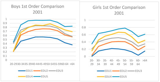
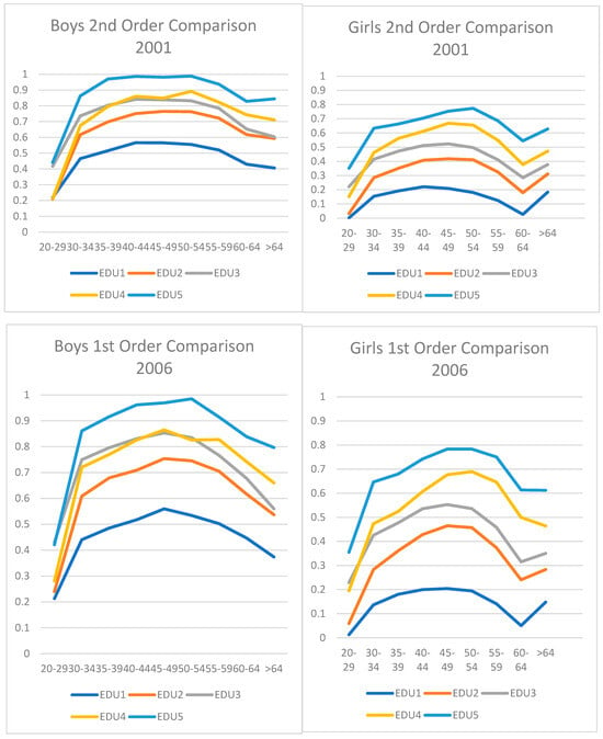
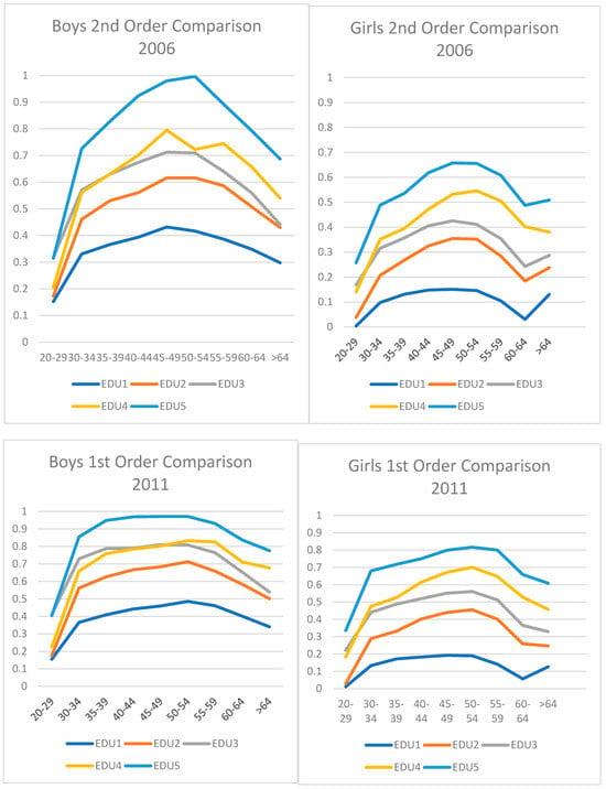
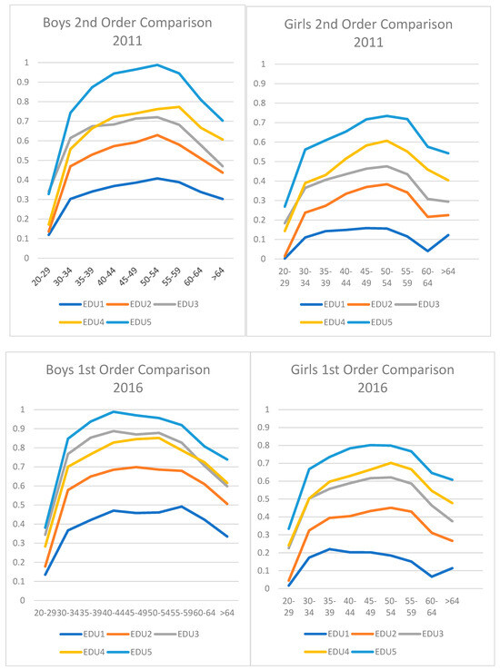
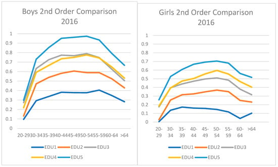
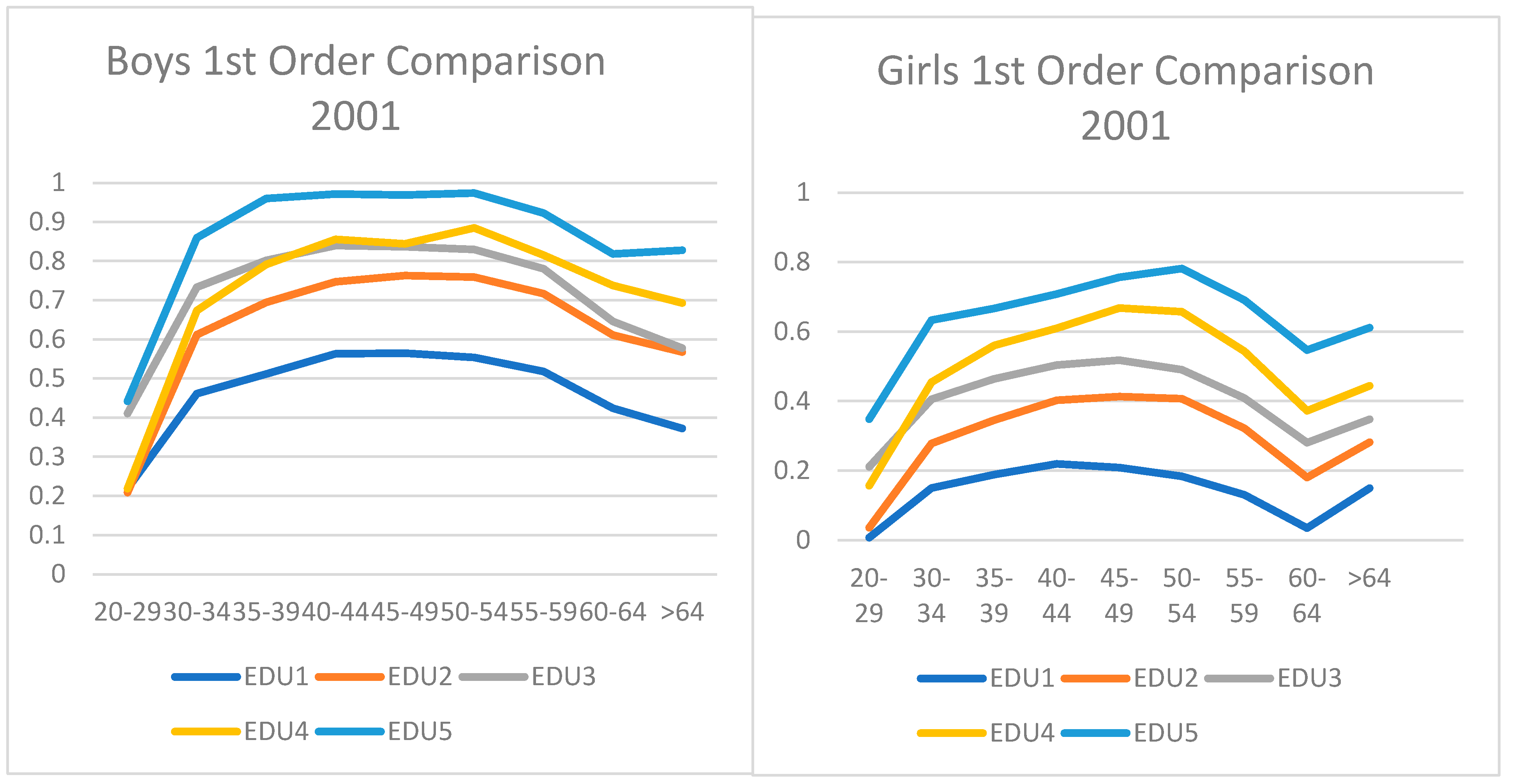
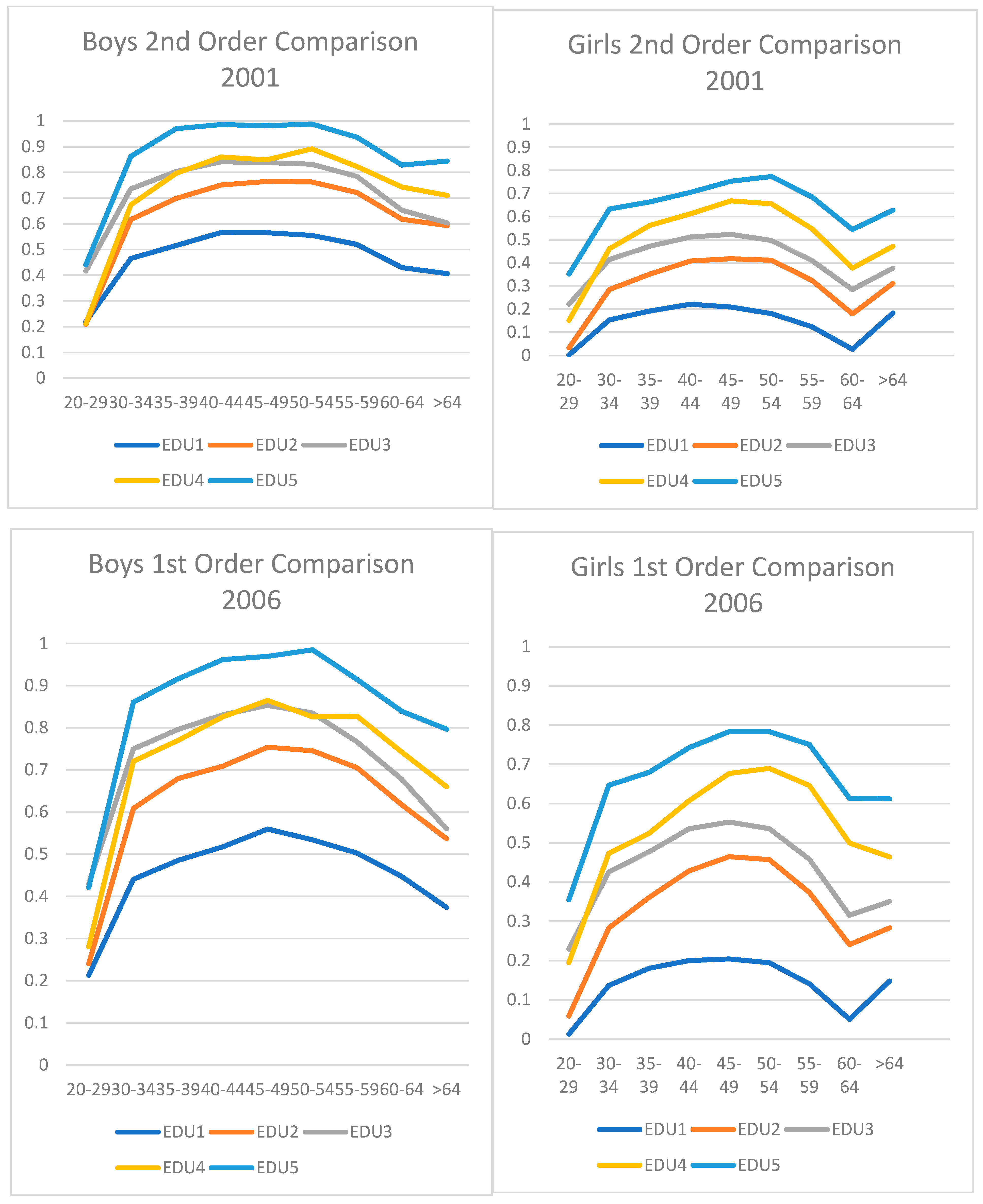
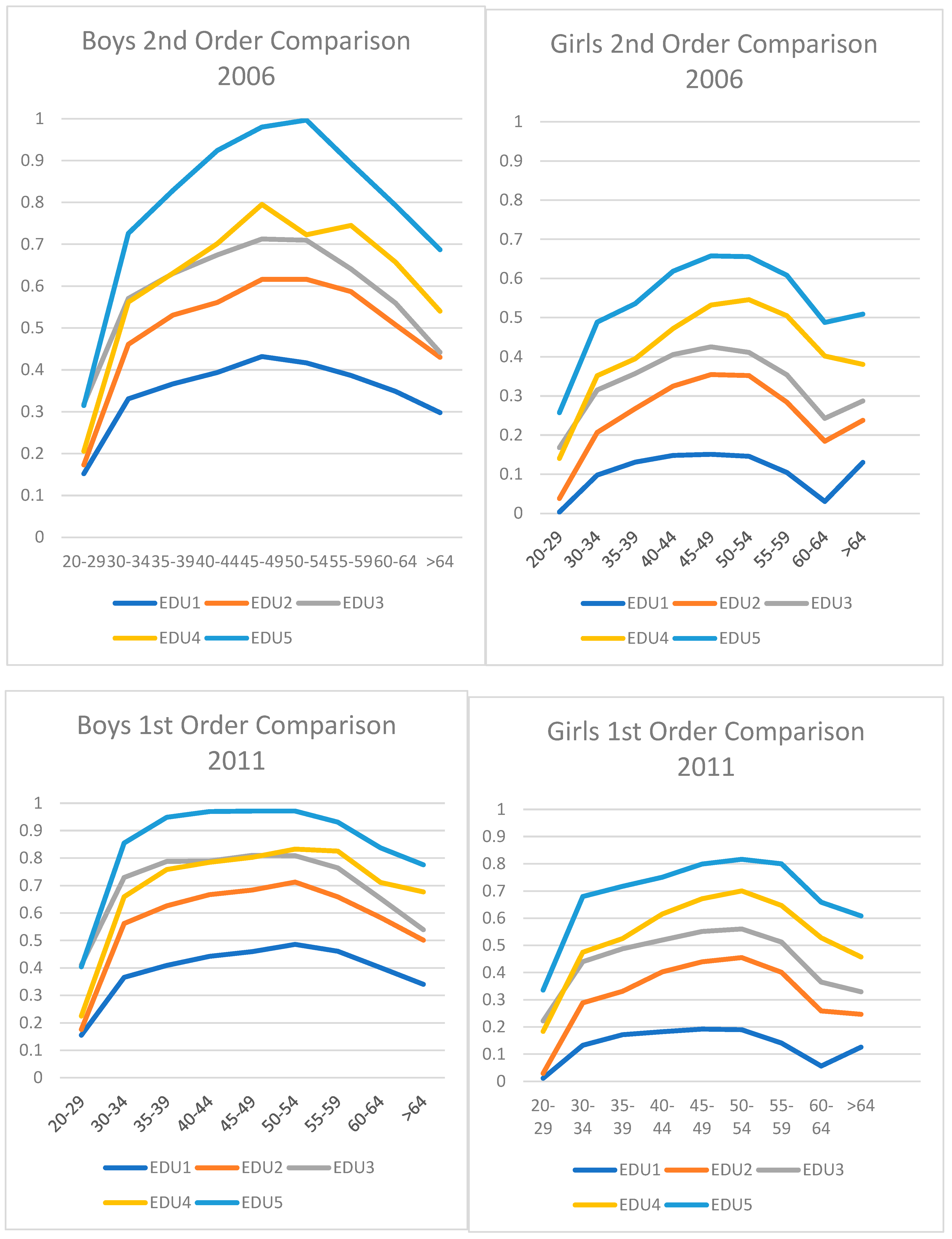
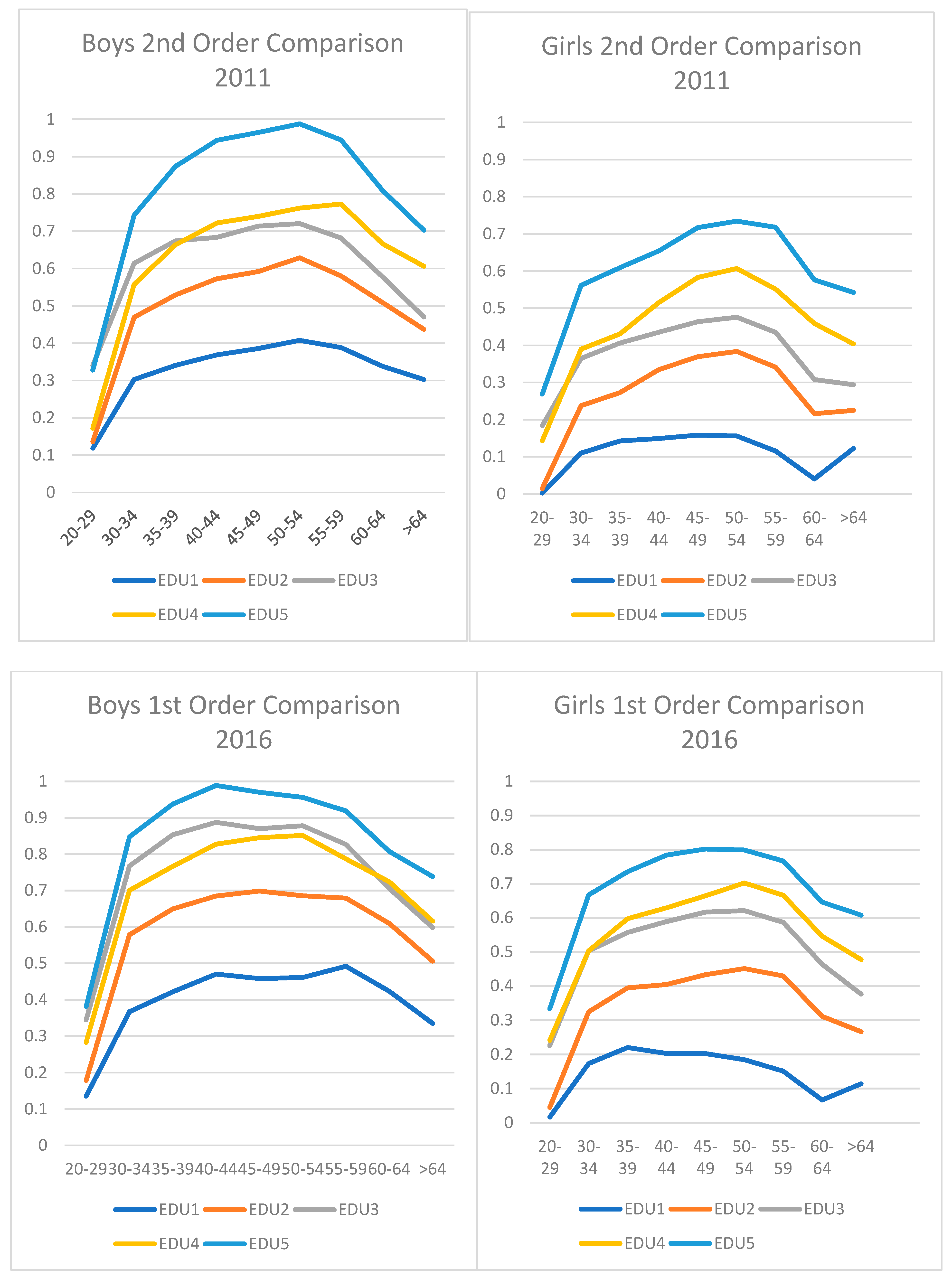
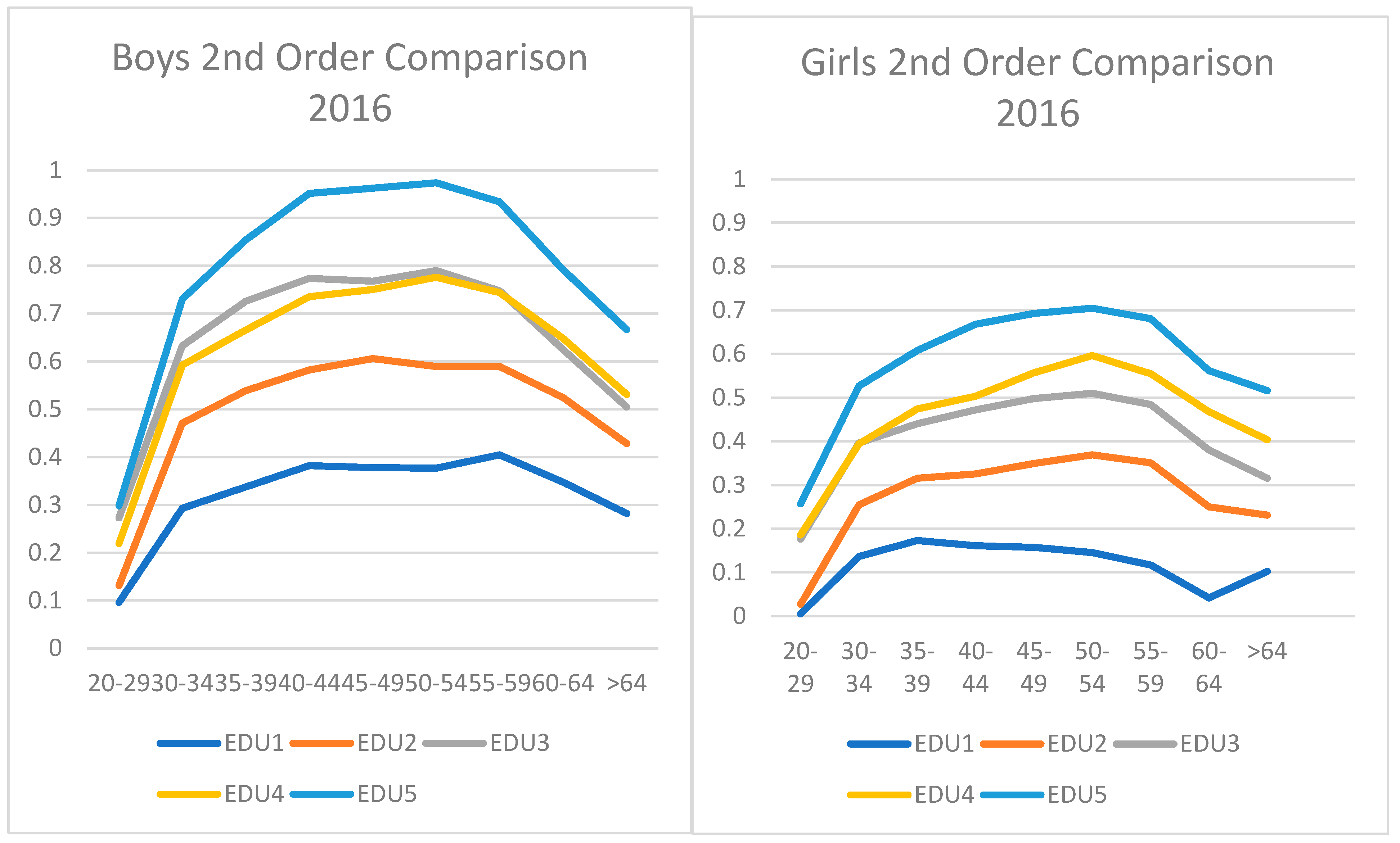
Initially, first- and second-order utopia–dystopia comparison indices, reported in Table A2 in the Appendix A, were calculated across all groups defined by the education and training (human capital) status and age group (experience) status categories. Table A2 is best visualized in the following Figure 1 that track the human capital status conditional utopia–dystopia income value index profiled over the various age (experience) groups. Generically, the profiles appear to peak in the late 40s–early 50s and typically, higher human capital-based profiles peak later than lower human capital-based profiles (i.e., the higher the level of human capital investment, the further in the future is the peak return). It also appears that, across the human capital spectrum, boys’ profiles peak earlier than girls’ profiles and that boys’ profiles are universally higher than the corresponding girls’ profiles. The peaks probably have something to do with the aging process; health declines with age, which will affect income-generating capacity, especially in profiles where physical effort is important. Furthermore, with technological progress, some skills embodied early in the work–life cycle can become obsolescent later in the work–life cycle (for example, the recent evolution in Artificial Intelligence has made some search skills redundant in many professions (Patel and Shah 2022; Vrontis et al. 2022)).

Figure 1. Work-Life Stage Relative income profiles.

To assess the work–lifetime differences, the average life-cycle stage difference and the average discounted present value weighted life-cycle stage difference using a 3% pa discount rate (in line with Canada’s growth rate over the period) were reported for both value function types together with ADIF1, the unambiguity in difference measures for the mean difference comparison. To obtain a sense of trends in the variation in rewards over the period, Table 2 reports the extreme work–life-cycle profile comparisons (effectively ED5 with ED1) both overall and within gender.

Table 2. Comparison of extremes.

	Best–Worst Comparisons
	Overall	Boys	Girls
2001 first-order comparison
Mean difference	0.7188	0.1432	0.2617
Present value weighted mean difference	0.8036	0.1467	0.3015
Difference unambiguity	1.0000	1.0000	1.0000
2001 second-order comparison
Mean difference	0.7275	0.1479	0.2692
Present value weighted mean difference	0.813	0.1514	0.3113
Difference unambiguity	1.0000	1.0000	1.0000
2006 first-order comparison
Mean difference	0.7107	0.1294	0.2904
Present value weighted mean difference	0.7936	0.126	0.335
Difference unambiguity	1.0000	0.9848	1.0000
2006 second-order comparison
Mean difference	0.689	0.2095	0.2248
Present value weighted mean difference	0.7567	0.2119	0.2579
Difference unambiguity	1.0000	0.9967	1.0000
2011 first-order comparison
Mean difference	0.7178	0.1524	0.3094
Present value weighted mean difference	0.8015	0.1526	0.3527
Difference unambiguity	1.0000	0.9901	1.0000
2011 second-order comparison
Mean difference	0.7003	0.2025	0.2632
Present value weighted mean difference	0.7699	0.2025	0.2992
Difference unambiguity	1.0000	0.9865	1.0000
2016 first-order comparison
Mean difference	0.6904	0.0906	0.3564
Present value weighted mean difference	0.7673	0.0958	0.3963
Difference unambiguity	1.0000	1.0000	1.0000
2016 second-order comparison
Mean difference	0.6802	0.1468	0.2925
Present value weighted mean difference	0.7423	0.1507	0.3231
Difference unambiguity	1.0000	1.0000	1.0000

The differences are mostly unambiguous, with discounted present value weighted average differences, which weight near-term differences more heavily than long-term differences, invariably larger. Over the 2006–2016 decade9, the overall differences appear to diminish over time, more so for Type 2 risk-averse value functions, indicating that the gap between the highest profile (boys ED5) and the lowest profile (girls ED1) is narrowing, indicating lower variability across career choices in future income rewards. Differences appear to have an inverted U profile within boy groups with the highest vs lowest gap narrowing over time. For girls, the highest vs lowest average gap is monotonic increasing at the first-order comparison.

To assess the work–life-cycle benefits of a one-level higher education and training choice, Table 3 reports the average life-cycle stage and average discounted present value weighted differences for both value function types together with the corresponding unambiguity in difference measures for each comparison for girls and boys. For both girls and boys, the choice over the work–life cycle is unambiguous for all but the ED3–ED4 decision, recording a work–life-cycle benefit to a one-category improvement in every case. Worthy of note is the fact that, at the lower end of the education and training spectrum, the differentials appear to diminish when viewed under a risk-averse rather than a risk-neutral lens, whereas at the upper end, they increase. Thus, for boys, the benefit of ED5 investment over an ED4 investment is even clearer under a risk-averse view of the world whereas for girls, the benefit of ED2 investment over an ED1 investment is somewhat less clear under a risk-averse view. Regarding the ED3–ED4 choice, a close to unambiguous improvement is recorded for girls but is extremely ambiguous for boys, always recording a disadvantage when considered in discounted present value terms, suggesting the short-term benefits of a trade or profession outweigh the long-term advantages of obtaining a basic bachelor’s degree. Table 4 reports the first-order unambiguity measures for each age group comparison for each education level, which, with the exception of the ED3–ED4 comparison for boys, indicates very little ambiguity in the individual comparisons overall and, since first-order dominance implies second-order dominance, there will be even less ambiguity in the second-order comparisons.

Table 3. Education and training level average and discounted present value weighted average differences over the work–life cycle.

	Girls				Boys
	ED2–ED1	ED3–ED2	ED4–ED3	ED5–ED4	ED2–ED1	ED3–ED2	ED4–ED3	ED5–ED4
2001 first-order difference
Mean difference	0.1546	0.1070	0.0929	0.1419	0.1657	0.0862	0.0066	0.1365
TP weighted mean difference	0.1644	0.1371	0.0870	0.1680	0.1695	0.1234	−0.0299	0.1766
Difference unambiguity	1.0000	1.0000	0.8850	1.0000	0.9865	1.0000	0.1022	1.0000
2001 second-order difference
Mean difference	0.1590	0.1102	0.0883	0.1366	0.1659	0.0858	0.0057	0.1422
TP weighted mean difference	0.1692	0.1421	0.0798	0.1639	0.1702	0.1234	−0.0319	0.1833
Difference unambiguity	1.0000	1.0000	0.8498	1.0000	0.9870	1.0000	0.0860	1.0000
2006 first-order comparison
Mean difference	0.1870	0.1034	0.0994	0.1322	0.1690	0.1005	0.0020	0.1273
TP weighted mean difference	0.2000	0.1349	0.0870	0.1621	0.1812	0.1375	−0.0269	0.1529
Difference unambiguity	1.0000	1.0000	0.9285	1.0000	1.0000	1.0000	0.0401	1.0000
2006 second-order comparison
Mean difference	0.1452	0.0796	0.0842	0.1216	0.1509	0.0861	0.0336	0.1759
TP weighted mean difference	0.1544	0.1035	0.0739	0.1451	0.1593	0.1155	0.0110	0.2009
Difference unambiguity	1.0000	1.0000	0.9316	1.0000	1.0000	1.0000	0.5557	1.0000
2011 first-order comparison
Mean difference	0.1833	0.1261	0.0905	0.1514	0.1835	0.1247	−0.0018	0.1542
TP weighted mean difference	0.1919	0.1608	0.0783	0.1826	0.1988	0.1695	−0.0403	0.1929
Difference unambiguity	1.0000	1.0000	0.9141	1.0000	1.0000	1.0000	−0.0285	1.0000
2011 second-order comparison
Mean difference	0.1553	0.1079	0.0796	0.1443	0.1668	0.1136	0.0208	0.1817
TP weighted mean difference	0.1614	0.1378	0.0671	0.1700	0.1792	0.1523	−0.0140	0.2165
Difference unambiguity	1.0000	1.0000	0.8984	1.0000	1.0000	1.0000	0.2845	1.0000
2016 first-order comparison
Mean difference	0.1919	0.1645	0.0542	0.1237	0.1898	0.1624	−0.0367	0.1273
TP weighted mean difference	0.1982	0.1981	0.0494	0.1462	0.2089	0.2000	−0.0553	0.1511
Difference unambiguity	1.0000	1.0000	1.0000	1.0000	1.0000	1.0000	−0.8198	1.0000
2016 second-order comparison
Mean difference	0.1593	0.1333	0.0516	0.1198	0.1737	0.1533	−0.0198	0.1667
TP weighted mean difference	0.1632	0.1599	0.0461	0.1378	0.1892	0.1852	−0.0350	0.1857
Difference unambiguity	1.0000	1.0000	0.9907	1.0000	1.0000	1.0000	−0.6422	1.0000

Table 4. Education level income distribution first-order comparison unambiguity measures10.

	Boys						Girls
	ED1–ED2	ED2–ED3	ED3–ED4	ED4–ED5	Age Group Average ED3–ED4 Omitted		ED1–ED2	ED2–ED3	ED3–ED4	ED4–ED5	Age Group Average
2001
20–29	−0.5625	1.0000	−1.0000	1.0000	0.1094	0.4791	1.0000	1.0000	−0.6866	1.0000	0.5784
30–34	1.0000	1.0000	−0.9046	1.0000	0.5239	1.0000	1.0000	1.0000	0.9978	1.0000	0.9994
35–39	1.0000	1.0000	−0.3065	1.0000	0.6734	1.0000	1.0000	1.0000	0.9888	0.9890	0.9944
40–44	1.0000	1.0000	0.5297	1.0000	0.8824	1.0000	1.0000	1.0000	1.0000	0.9868	0.9967
45–49	1.0000	1.0000	0.5661	0.9978	0.8910	0.9992	1.0000	1.0000	1.0000	0.9776	0.9944
50–54	1.0000	1.0000	1.0000	0.9990	0.9998	0.9996	1.0000	1.0000	1.0000	1.0000	1.0000
55–59	1.0000	1.0000	0.7724	1.0000	0.9431	1.0000	1.0000	0.9984	1.0000	0.9942	0.9982
60–64	1.0000	0.9523	0.9391	1.0000	0.9728	0.9841	1.0000	1.0000	1.0000	1.0000	1.0000
≥65	1.0000	0.2757	0.9635	0.9972	0.8091	0.7576	1.0000	0.9993	1.0000	0.9881	0.9969
ED level Average	0.8264	0.9142	0.2844	0.9993	0.7561	0.9133	1.0000	0.9997	0.8111	0.9929	0.9509
2006
20–29	0.9978	1.0000	−0.9985	1.0000	0.4998	0.9992	1.0000	0.9993	−0.5720	1.0000	0.6068
30–34	1.0000	1.0000	−0.6340	0.9965	0.5906	0.9988	1.0000	1.0000	0.6777	1.0000	0.9194
35–39	1.0000	1.0000	−0.5873	1.0000	0.6032	1.0000	1.0000	1.0000	0.7176	1.0000	0.9294
40–44	1.0000	1.0000	−0.1232	1.0000	0.7192	1.0000	1.0000	1.0000	0.9602	1.0000	0.9900
45–49	1.0000	1.0000	0.2136	1.0000	0.8034	1.0000	1.0000	1.0000	1.0000	0.9908	0.9977
50–54	1.0000	1.0000	−0.2690	1.0000	0.6827	1.0000	1.0000	1.0000	1.0000	0.9696	0.9924
55–59	1.0000	1.0000	0.9885	1.0000	0.9971	1.0000	1.0000	1.0000	1.0000	1.0000	1.0000
60–64	1.0000	1.0000	0.9630	0.9858	0.9872	0.9952	1.0000	1.0000	1.0000	1.0000	1.0000
≥65	0.9930	0.7065	0.8603	0.9767	0.8841	0.8920	1.0000	1.0000	0.9928	0.9886	0.9953
ED level Average	0.9990	0.9674	0.0459	0.9954	0.7519	0.9872	1.0000	0.9999	0.7529	0.9943	0.9368
2011
20–29	0.9813	1.0000	−1.0000	1.0000	0.4953	0.9937	0.6057	1.0000	−0.5568	1.0000	0.5122
30–34	1.0000	1.0000	−0.8936	1.0000	0.5266	1.0000	1.0000	1.0000	0.5503	1.0000	0.8876
35–39	1.0000	1.0000	−0.5393	1.0000	0.6152	1.0000	1.0000	1.0000	0.6490	1.0000	0.9123
40–44	1.0000	1.0000	−0.0830	1.0000	0.7292	1.0000	1.0000	1.0000	0.9595	1.0000	0.9899
45–49	1.0000	1.0000	−0.1561	1.0000	0.7110	1.0000	1.0000	1.0000	1.0000	1.0000	1.0000
50–54	1.0000	1.0000	0.7037	1.0000	0.9259	1.0000	1.0000	1.0000	1.0000	1.0000	1.0000
55–59	1.0000	1.0000	0.8327	1.0000	0.9582	1.0000	1.0000	1.0000	0.9992	1.0000	0.9998
60–64	1.0000	1.0000	0.8770	1.0000	0.9692	1.0000	1.0000	1.0000	1.0000	1.0000	1.0000
≥65	0.9875	1.0000	0.9431	0.9657	0.9741	0.9844	1.0000	1.0000	0.9987	0.9930	0.9979
ED level Average	0.9965	1.0000	0.0761	0.9962	0.7672	0.9976	0.9562	1.0000	0.7333	0.9992	0.9222
2016
20–29	1.0000	1.0000	−1.0000	1.0000	0.5000	1.0000	0.9292	0.9998	0.4485	1.0000	0.8444
30–34	1.0000	1.0000	−0.9690	1.0000	0.5078	1.0000	1.0000	1.0000	0.0035	0.9976	0.7503
35–39	1.0000	1.0000	−0.9849	1.0000	0.5038	1.0000	1.0000	0.9989	0.8324	0.9885	0.9549
40–44	1.0000	1.0000	−0.9443	1.0000	0.5139	1.0000	1.0000	1.0000	0.6887	1.0000	0.9222
45–49	1.0000	1.0000	−0.7268	1.0000	0.5683	1.0000	1.0000	1.0000	0.8317	1.0000	0.9579
50–54	1.0000	1.0000	−0.9650	0.9985	0.5084	0.9995	1.0000	1.0000	0.9912	0.9826	0.9935
55–59	1.0000	1.0000	−0.7841	0.9989	0.5537	0.9996	1.0000	1.0000	0.9823	1.0000	0.9956
60–64	1.0000	1.0000	0.4126	1.0000	0.8531	1.0000	1.0000	1.0000	1.0000	1.0000	1.0000
≥65	0.9843	1.0000	0.6044	0.9482	0.8842	0.9775	1.0000	1.0000	1.0000	0.9635	0.9909
ED level Average	0.9983	1.0000	−0.5952	0.9940	0.5992	0.9974	0.9921	0.9999	0.7531	0.9925	0.9344

Perhaps the most striking set of comparisons are presented in Table 5, which reports the work–life-cycle differences between girls and boys at each education level. Again, present value weighted mean differences, which weight near-term advantages more heavily than long-term advantages, are invariably larger than simple mean differences, and all are completely unambiguous and all favor Boys; in essence, there is a universal male premium in future income value. However, the premium, which appears to be larger at the lower end of the education and training spectrum than at the upper end, is diminishing over time whether viewed through a risk-neutral Type 1 value function lens or a risk-averse Type 2 value function lens, probably a reflection of the “Grand Gender Convergence” observed by Goldin (2014) and a sign of the improving fortunes of girls. However, though girls appear to be catching up, they are still at a disadvantage throughout the education training and experience spectrum.

Table 5. Gender differences.

	ED1	ED2	ED3	ED4	ED5
2001 first-order comparison
Mean difference	0.3238	0.3348	0.3140	0.2277	0.2224
Present value weighted mean difference	0.3639	0.3690	0.3553	0.2384	0.2470
Average difference ambiguity	1.0000	1.0000	1.0000	1.0000	1.0000
2001 second-order comparison
Mean difference	0.3279	0.3348	0.3104	0.2278	0.2334
TP weighted mean difference	0.3680	0.3689	0.3502	0.2385	0.2579
Average difference ambiguity	1.0000	1.0000	1.0000	1.0000	1.0000
2006 first-order comparison
Mean difference	0.3118	0.2938	0.2909	0.1935	0.1886
TP weighted mean difference	0.3489	0.3301	0.3327	0.2187	0.2095
Average difference ambiguity	1.0000	1.0000	1.0000	1.0000	1.0000
2006 second-order comparison
Mean difference	0.2424	0.2481	0.2547	0.2041	0.2584
TP weighted mean difference	0.2700	0.2749	0.2869	0.2241	0.2798
Average difference ambiguity	1.0000	1.0000	1.0000	1.0000	1.0000
2011 first-order comparison
Mean difference	0.2572	0.2574	0.2560	0.1637	0.1665
TP weighted mean difference	0.2806	0.2875	0.2962	0.1776	0.1879
Average difference ambiguity	1.0000	1.0000	1.0000	1.0000	1.0000
2011 second-order comparison
Mean difference	0.2174	0.2288	0.2346	0.1757	0.2131
TP weighted mean difference	0.2358	0.2536	0.2681	0.1870	0.2335
Average difference ambiguity	1.0000	1.0000	1.0000	1.0000	1.0000
2016 first-order comparison
Mean difference	0.2477	0.2456	0.2434	0.1525	0.1561
TP weighted mean difference	0.2625	0.2732	0.2752	0.1705	0.1754
Average difference ambiguity	1.0000	1.0000	1.0000	1.0000	1.0000
2016 second-order comparison
Mean difference	0.2064	0.2208	0.2408	0.1694	0.2163
TP weighted mean difference	0.2171	0.2431	0.2685	0.1873	0.2352
Average difference ambiguity	1.0000	1.0000	1.0000	1.0000	1.0000

8. Conclusions

Throughout an individual’s work–life cycle, their income stream is the reward for the efforts they expend in applying their human resource stock (the amorphous mixture of innate abilities, education, training and experience they have acquired) in productive activity. At each stage of the cycle, the nature of the human resource stock will depend a great deal on the choices made at an earlier stage. Indeed, most investment choices are made early in the life-cycle path, often long before the outcomes predicated upon those choices will be realized, which makes assessing the comparative advantage of different investment choices over that path challenging. It involves comparison of path-contingent income distributions in their entirety at each stage of the work–life cycle with theoretic choice considerations indicating that differences should be valued differently dependent upon whether they are viewed through a risk-neutral or a risk-averse lens. Furthermore, when distributions of different groups are proximate, comparisons can be ambiguously equivocal and clear advantages of different paths become difficult to elicit. Here, a methodology is proposed for making such comparisons and evaluating their potential for ambiguity. The techniques have been applied to the recipients of incomes over the age of 19 in 21st-century Canada.

By and large, restricting the income value function to risk-averting preferences had little effect on the orderings and the higher the level of education and training received, the higher will the income value profile be throughout the work–life cycle, whether viewed through a risk-neutral or a risk-averse lens. Furthermore, for the most part, these differences are unambiguous and unequivocal. Generally, the biggest incremental impact on income profiles is the move from no high school certificate to graduating high school with a certificate or diploma. The only contentious life-cycle choice is that between obtaining a trade or apprenticeship certificate versus a basic university degree (and nothing more) and for boys, it is at best a marginal choice, whereas for girls, the choice is much clearer, with a university degree trumping a trade or apprenticeship. Of particular interest to policy makers concerned with gender equity issues is that, on the assumption that the proclivity for effort is identically distributed across the genders, boys enjoy a substantial premium at all human resource levels, though the gaps do appear to be narrowing over time, consistent with a Grand Gender Convergence (Goldin 2014).

With regard to future research, aside from seeing if similar results prevail in other jurisdictions, it would be interesting to examine a more comprehensive breakdown of human resource stock structures that included professional networks and health considerations, for example.

References

- Anderson, Gordon. 1996. Nonparametric Tests of Stochastic Dominance in Income Distributions. Econometrica 64: 1183–93. [Google Scholar] [CrossRef] [Scilit]
- Anderson, Gordon, and Teng Wah Leo. 2021. On Extending Stochastic Dominance Comparisons to Ordinal Variables and Generalising Hammond Dominance. University of Toronto Department of Economics Working Paper 705. Toronto: University of Toronto. [Google Scholar]
- Anderson, Gordon, Thierry Post, and Yoon-Jae Whang. 2020. Somewhere Between Utopia and Dystopia: Choosing from Multiple Incomparable Prospects. Journal of Business and Economic Statistics 38: 502–15. [Google Scholar] [CrossRef] [Scilit]
- Barrett, Garry, and Stephen Donald. 2003. Consistent Tests for Stochastic Dominance. Econometrica 71: 71–104. [Google Scholar] [CrossRef] [Scilit]
- Becker, Gary, and Barry Chiswick. 1966. Education and the Distribution of Earnings. American Economic Review 56: 358–69. [Google Scholar]
- Bond, Timothy, and Kevin Lang. 2019. The Sad Truth about Happiness Scales. Journal of Political Economy 127: 1629–40. [Google Scholar] [CrossRef] [Scilit]
- Buchinsky, Moshe. 1998. Recent Advances in Quantile Regression Models: A Practical Guide for Empirical Research. The Journal of Human Resources 33: 88–126. [Google Scholar] [CrossRef] [Scilit]
- Byrne, Kaileigh, and Darrell Worthy. 2015. Gender differences in reward sensitivity and information processing during decision making. Journal of Risk and Uncertainty 50: 55–71. [Google Scholar] [CrossRef] [Scilit]
- Cantril, Hadley. 1965. The Pattern of Human Concerns. New Brunswick: Rutgers University Press. [Google Scholar]
- Carneiro, Pedro, Karsten Hansen, and James Heckman. 2003. Lawrence R. Klein Lecture. Estimating Distributions of Treatment Effects with an Application to the Returns to Schooling and Measurement of the Effects of Uncertainty on College Choice. International Economic Review 44: 361–422. [Google Scholar] [CrossRef] [Scilit]
- Case, Anne, and Christina Paxson. 2005. Sex differences in morbidity and mortality. Demography 42: 189–214. [Google Scholar] [CrossRef] [Scilit]
- Croson, Rachel, and Uri Gneezy. 2009. Gender differences in preferences. Journal of Economic Literature 47: 448–598. [Google Scholar] [CrossRef] [Scilit]
- Davidson, Russell, and Jean-Yves Duclos. 2000. Statistical Inference for Stochastic Dominance and for the Measurement of Poverty and Inequality. Econometrica 68: 1435–64. [Google Scholar] [CrossRef] [Scilit]
- Deaton, Angus, and Christina Paxson. 1998. Aging and inequality in income and health. The American Economic Review 88: 248–53. [Google Scholar]
- Dwyer, Peggy, James Gilkerson, and John List. 2002. Gender differences in revealed risk taking: Evidence from mutual fund investors. Economics Letters 76: 151–58. [Google Scholar] [CrossRef] [Scilit]
- Goldin, Claudia. 2014. A Grand Gender Convergence: Its Last Chapter. American Economic Review 104: 1–30. [Google Scholar] [CrossRef] [Scilit]
- Hall, Peter, and Adonis Yatchew. 2005. Unified Approach to Testing Functional Hypothesis in Semiparametric Contexts. Journal of Econometrics 127: 225–52. [Google Scholar] [CrossRef] [Scilit]
- Kahneman, Daniel, and Amos Tversky. 1979. Prospect Theory: An Analysis of Decision Under Risk. Econometrica 47: 263–91. [Google Scholar]
- Kerkhofs, Marcel, and Maarten Lindeboom. 1997. Age Related Health Dynamics and Changes in Labour Market Status. Health Economics 6: 407–23. [Google Scholar] [CrossRef]
- Leshno, Moshe, and Haim Levy. 2002. Preferred by “All” and Preferred by “Most” Decision Makers: Almost Stochastic Dominance. Management Science 48: 1074–85. [Google Scholar] [CrossRef] [Scilit]
- Levy, Haim. 1998. Stochastic Dominance: Investment Decision Making Under Uncertainty. Alphen aan den Rijn: Kluwer Academic Publishers. [Google Scholar]
- Linton, Oliver, Esfandiar Maasoumi, and Yoon-Jae Whang. 2005. Consistent Testing for Stochastic Dominance under General Sampling Schemes. Review of Economic Studies 72: 735–65. [Google Scholar] [CrossRef] [Scilit]
- Miller, Ray, and Neha Bairoliya. 2023. Health, Longevity, and Welfare Inequality of Older Americans. The Review of Economics and Statistics 105: 1145–60. [Google Scholar] [CrossRef] [Scilit]
- Nusselder, W., C. Looman, H. Van Oyen, J. M. Robine, and C. Jagger. 2010. Gender differences in health of EU10 and EU15 populations: The double burden of EU10 men. European Journal of Ageing 7: 219–27. [Google Scholar] [CrossRef] [Scilit]
- Oksuzyan, Anna, Inge Petersen, Henrik Stovring, Paul Bingley, James Vaupel, and Kaare Christensen. 2009. The male-female health–survival paradox: A survey and register study of the impact of sex-specific selection and information bias. Annals of Epidemiology 19: 504–11. [Google Scholar] [CrossRef] [Scilit]
- Patel, Veer, and Manan Shah. 2022. Artificial intelligence and machine learning in drug discovery and development. Intelligent Medicine 2: 134–40. [Google Scholar] [CrossRef] [Scilit]
- Schroder, Carsten, and Shlomo Yitzhaki. 2017. Revisiting the evidence for cardinal treatment of ordinal variables. European Economic Review 92: 337–58. [Google Scholar] [CrossRef] [Scilit]
- Van Oyen, Herman, Wilma Nusselder, Carol Jagger, Petra Kolip, Emmanuelle Cambois, and Jean-Marie Robine. 2013. Gender differences in healthy life years within the EU: An exploration of the “health–survival” paradox. International Journal of Public Health 58: 143–55. [Google Scholar] [CrossRef] [Scilit]
- Vrontis, Demitris, Michael Christofi, Vijay Pereira, Shlomo Tarba, Anna Makrides, and Eleni Trichina. 2022. Artificial intelligence, robotics, advanced technologies and human resource management: A systematic review. The International Journal of Human Resource Management 33: 1237–66. [Google Scholar] [CrossRef] [Scilit]
- Whang, Yoon-Jae. 2019. Econometric Analysis of Stochastic Dominance: Concepts, Methods, Tools and Applications. Cambridge: Cambridge University Press. [Google Scholar] [CrossRef] [Scilit]
Disclaimer/Publisher’s Note: The statements, opinions and data contained in all publications are solely those of the individual author(s) and contributor(s) and not of MDPI and/or the editor(s). MDPI and/or the editor(s) disclaim responsibility for any injury to people or property resulting from any ideas, methods, instructions or products referred to in the content. |
© 2024 by the author. Licensee MDPI, Basel, Switzerland. This article is an open access article distributed under the terms and conditions of the Creative Commons Attribution (CC BY) license (https://creativecommons.org/licenses/by/4.0/).