


Abstract
Stressis a psychological state that significantly impacts mental and cardiovascular health when prolonged, making continuous wearable monitoring valuable. Photoplethysmography (PPG) signals are especially practical, yet existing PPG-based stress-detection methods rely on long data segments (30 s or longer), whereas recent PPG-based research increasingly adopts 10 s windows. Moreover, strict subject-independent evaluation reveals substantial performance degradation due to inter-subject physiological variability, while stress labels are rarely available for new users. To address these challenges, this work proposes a short-term PPG stress detection framework. A backbone is first pre-trained on VitalDB, a large-scale clinical PPG dataset that carries no stress labels; we show that such stress-label-free pre-training—which short-term stress-detection methods have not exploited—still transfers to downstream stress detection. This backbone then feeds a Personalized Expert Routing (PER) module, which routes each sample to specialized expert networks. Routing is guided by two complementary signals—the user’s resting-state PPG features and the current signal’s content—so the model adapts to individual differences without new-user stress labels. Under subject-independent 5-fold cross-validation on WESAD, CATSA, and CLAS, the proposed method achieves an average F1-score of 0.6919, an average area under the receiver operating characteristic curve (AUC) of 0.7521, and an average accuracy of 0.6883, outperforming the strongest baseline by 4.14, 4.67, and 3.12 percentage points, respectively.
1. Introduction
Stress is defined by the World Health Organization as a state of worry or mental tension caused by a difficult situation [1]. Prolonged exposure to high levels of psychological stress significantly increases the risk of developing depression and even cardiovascular diseases [2]. Consequently, continuous monitoring of stress states holds substantial practical value in assisting individuals with psychological self-regulation. While numerous studies have explored emotion and stress detection based on modalities such as text, facial expressions, images, and videos [3], these approaches often encounter considerable challenges in practical deployment and real-world generalization. In light of this, subsequent research has shifted toward utilizing more objective and reliable physiological signals, including electroencephalography (EEG), electrocardiography (ECG), electromyography (EMG), photoplethysmography (PPG), electrodermal activity (EDA), and skin temperature [4]. Among these modalities, PPG is especially attractive for continuous, wearable stress monitoring: it can be acquired with a single low-power optical sensor that is already ubiquitous in consumer smartwatches and fitness bands, without the intrusive electrode placement required by EEG or ECG. However, PPG signals are susceptible to motion artifacts and sensor variability, which can degrade signal quality and must be mitigated during preprocessing.
Existing research paradigms for processing and classifying PPG signals generally fall into two categories: traditional feature engineering and deep learning. Recent models developed through these approaches have routinely achieved high accuracy rates (up to approximately 98%) on public benchmark datasets [5,6,7].
Nevertheless, three primary limitations hinder practical deployment. First, most existing methods rely on data segments of 30 s or longer [5,6], whereas recent work increasingly analyzes 10 s windows [7,8,9]. Second, many studies do not strictly enforce subject-independent evaluation, and stress labels are rarely available for new users. Third, pre-training remains largely unexplored for short-term PPG stress detection: PPG foundation models [8,10,11] are not adapted to this subtask, and existing self-supervised pre-training [12] pre-trains on the same target datasets.
To address these limitations, this work makes the following contributions:
- To enhance information extraction from short-term (10 s) PPG segments while eliminating the risk of data leakage, we pre-train a backbone on a large-scale clinical PPG dataset, and empirically demonstrate that such pre-training improves downstream short-term stress detection.
- To account for significant inter-subject physiological variance and the practical challenge of missing stress labels, we propose a Personalized Expert Routing (PER) classification method that leverages easily obtainable resting-state PPG features as a prior to adaptively route samples to specialized experts.
- Extensive experiments under strict subject-independent 5-fold cross-validation on WESAD [13], CATSA [14], and CLAS [15] demonstrate that our method outperforms the strongest baseline by 4.14 percentage points in average F1-score and 4.67 percentage points in average AUC.
2. Related Work
The development of physiological stress detection has progressed from handcrafted feature engineering to end-to-end deep learning and, most recently, toward lightweight models suited to wearable devices. Early approaches extracted handcrafted physiological features—such as heart-rate-variability statistics and electrodermal activity measures—and combined them with classical classifiers, including support vector machines (SVMs) and Random Forests; a representative early example is the driving-stress study of Healey and Picard [16], which derived features from ECG, EMG, and EDA signals for supervised classification.
The advent of deep learning then enabled models to learn hierarchical representations directly from raw signals, removing the need for manual feature design. IEBDNN [17] encodes one-dimensional time series into two-dimensional Gramian Angular Field (GAF) images processed by a convolutional neural network (CNN). SADDNet [5] builds a lightweight network with dilated convolution, local attention, and separable convolution blocks for real-time stress detection from raw PPG, and ReTeNet [18] pairs a residual encoder with transformer encoders to balance representational capacity with computational efficiency.
To improve accuracy, some methods have combined handcrafted and learned representations. The leave-one-out cross-validation (LOOCV)-based method [19] concatenates handcrafted features with those extracted by a neural network before recursive feature elimination and XGBoost classification. The feature-augmented hybrid CNN of Rashid et al. [20] similarly injects statistical and morphological descriptors into the intermediate layers of a deep network.
In parallel, recent PPG-based research has increasingly adopted 10 s analysis windows, whereas most prior stress-detection work still relies on 30–120 s windows [5,6,20,21]. DilatedCNN [7], for instance, classifies 10 s raw PPG segments directly without preprocessing, and 10 s windows have likewise become common across other PPG-based studies [8,9,22,23]. Relatedly, a number of studies report high accuracy with subject-dependent or mixed splits that overestimate generalization—for instance, DilatedCNN partitions data at the window level, mixing the same subjects across training and test sets.
Beyond these detection approaches, pre-training has been used to learn general PPG representations from large-scale unlabeled data. Contrastive learning on 141K-participant Apple Watch data [10] and PPG foundation models such as PaPaGei [8] and SiamQuality [11] learn transferable representations for general health-monitoring tasks, yet none have been fine-tuned for short-term PPG stress detection. A recent self-supervised study by Yaseen and Şahin [12] applies masked signal modeling to stress and affect detection, but pre-trains on the target wearable datasets themselves (WESAD, SWELL-KW), uses 60 s multimodal windows, and does not specify whether held-out test subjects are excluded from pre-training—leaving a potential subject-level leakage risk. Whether pre-training on a separate clinical PPG dataset that carries no stress labels transfers to short-term (10 s), single-channel PPG stress detection therefore remains open; this is the question we address. We adopt VitalDB [24] as our pre-training data.
3. Materials and Methods
3.1. Overview
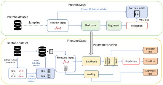
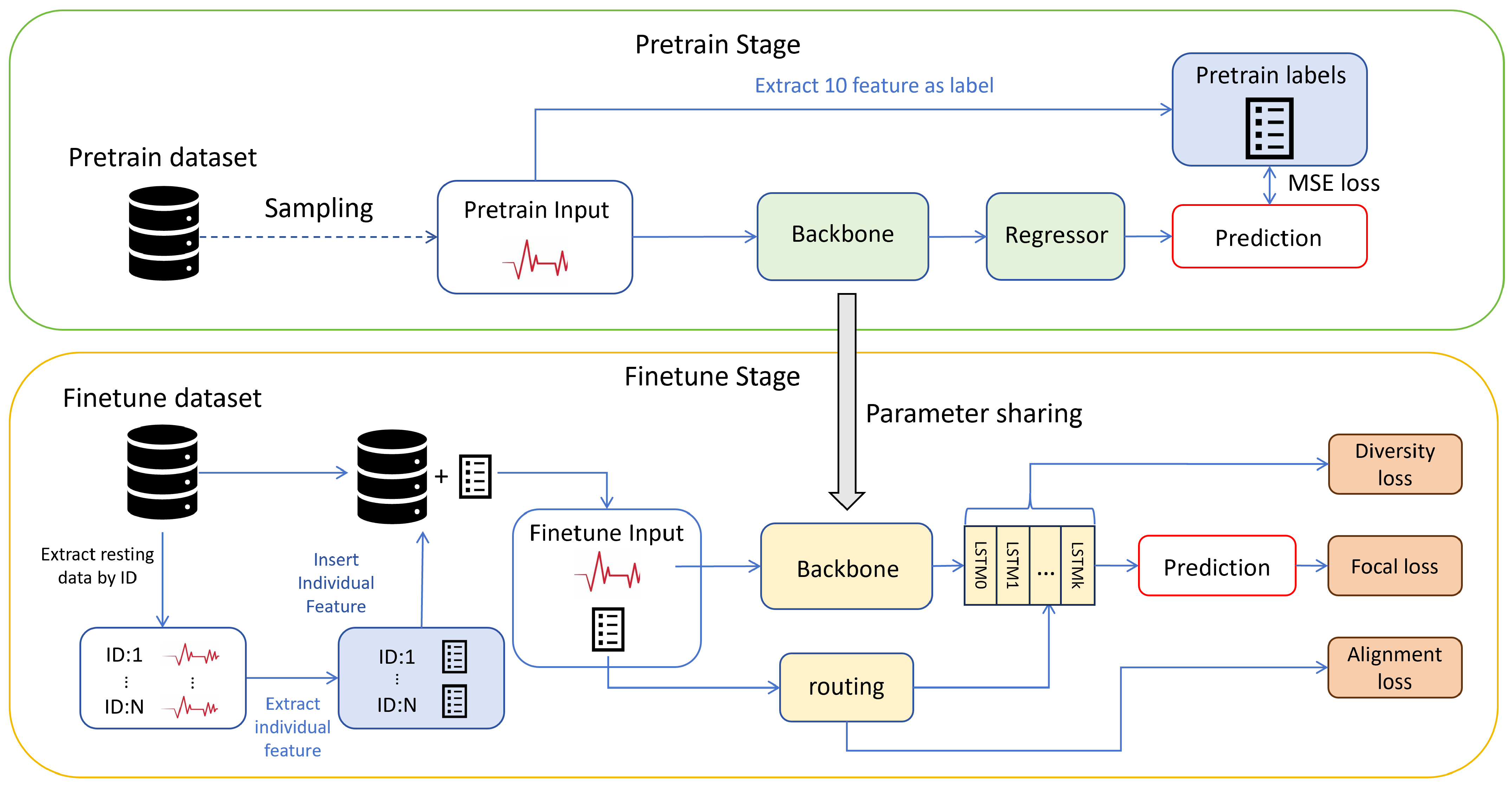
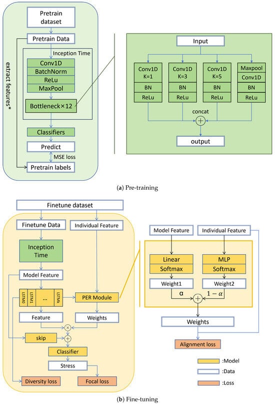
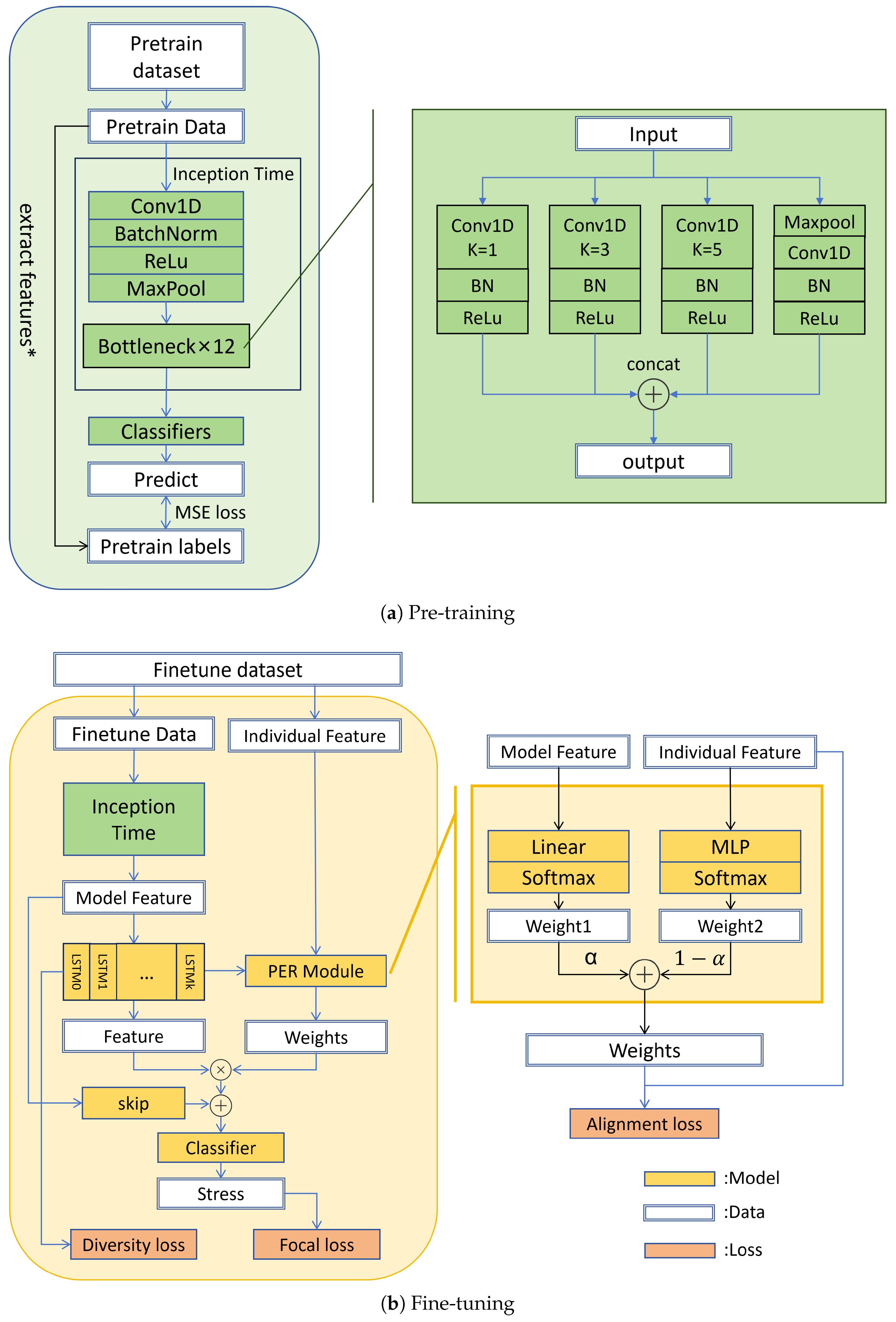
The overall architecture of our proposed method is illustrated in Figure 1, comprising three principal modules—a Pre-training Module, a Long Short-Term Memory (LSTM) Expert Module, and a Personalized Expert Routing (PER) Module—together with a lightweight domain adapter and a residual head-skip; the detailed pre-training and fine-tuning structures are shown in Figure 2. Initially, a multi-output pre-training strategy is conducted on VitalDB, a large-scale clinical PPG dataset: the backbone is trained to jointly regress ten interpretable PPG features—computed from each raw segment and used as the training labels—thereby learning physiologically meaningful representations from short-term PPG segments, with zero subject overlap with downstream benchmarks. Subsequently, the deepest feature map generated by the pre-trained backbone is adapted to the downstream domain by a lightweight residual domain adapter, and the adapted features are fed in parallel into multiple LSTM expert models to learn diverse temporal representations. The PER module then computes the weighting coefficients for each expert based on a combination of the current signal’s content and the individual’s resting-state PPG features. Finally, the outputs of all experts are aggregated via weighted summation, a global-average-pooled backbone feature is added as a residual head-skip, and the resulting representation is passed through a fully connected layer to produce the final stress classification result.
Figure 1.
Overall architecture of the proposed Personalized Expert Routing (PER) framework for short-term PPG stress detection. The pre-training stage pre-trains a backbone on VitalDB using interpretable physiological features as training labels. The fine-tuning stage applies a lightweight domain adapter to the backbone features, incorporates individual resting-state features and signal content to adaptively route samples to specialized LSTM experts, and adds a residual head-skip from the backbone global pooling to the classifier.
Figure 2.
Detailed structure of the pre-training and fine-tuning models. (a) Pre-training: InceptionTime backbone learns to regress ten interpretable PPG features on VitalDB; the ten pre-training targets (marked with *) are defined in Appendix B. (b) Fine-tuning: a zero-initialized domain adapter is applied to the deepest InceptionTime feature map, which then feeds K LSTM experts; the PER module computes routing weights from both the pre-trained features and individual resting-state features, and a head-skip adds a global-pooled backbone feature to the fused representation. Green shading highlights the pre-training stage (a) and the pre-trained backbone (b).
3.2. Pre-Training Module
The pre-training stage learns a backbone for extracting representations from short PPG segments by training it to regress interpretable physiological features on VitalDB. Specifically, the backbone is an InceptionTime architecture [25], whose output is mapped to ten PPG feature targets through a small regression head; once training converges, the head is discarded and only the backbone weights are retained for downstream fine-tuning. The detailed backbone structure and pre-training configuration are provided in Appendix C, while the label construction is described in Appendix B.
During downstream fine-tuning, the retained backbone is adapted to the target domain by a lightweight domain adapter: a zero-initialized pointwise () convolution with a residual connection applied to the deepest feature map. The adapter is an identity at initialization and thereafter learns channel-wise remixing at the full learning rate, while the backbone itself updates at a small learning rate.
Ten interpretable PPG features are used as regression targets [26,27]: two heart-rate (HR) features, two time-domain heart-rate-variability (HRV) indices computed on ultra-short windows, three pulse wave timing features, and three morphological features, as listed in Table A2 (Appendix B).
Pulse peaks are detected on the detrended signal with a minimum inter-peak distance of 0.5 s, and outlying pulse intervals (beyond ) are discarded. The 0.5 s threshold corresponds to an upper bound of 120 bpm and avoids spurious peaks, improving the reliability of peak detection. This value is carefully chosen, because the recordings on which peak detection is performed maintain low and stable heart rates. Features are then computed from the available peaks and set to zero when not computable.
3.3. LSTM Expert Module
For temporal modeling of the short 10 s segments, we adopt LSTM rather than Transformer encoders: our experiments found that the Transformer offers no accuracy advantage on such short sequences—the LSTM even slightly outperforms it—while requiring fewer parameters. The three encoders—unidirectional LSTM, bidirectional Gated Recurrent Unit (GRU), and Transformer—are compared under identical settings in Table A9. Different individuals may exhibit distinct patterns of physiological change under stress, so we employ multiple independently initialized LSTM experts to encourage each expert to converge to complementary temporal representations: some experts may become sensitive to rapid, transient fluctuations (e.g., a sudden rise in heart rate), whereas others may attend to slower trends (e.g., gradual recovery after a stressor). By maintaining a pool of specialized temporal encoders, the subsequent PER router can selectively activate the expert(s) most relevant to the current input and the individual’s physiological profile, thereby improving both accuracy and interpretability. The specific expert count, hidden size, and initialization schemes are provided in Appendix C.
3.4. Personalized Expert Routing (PER) Module
The architecture of the proposed PER module, inspired by the mixture-of-experts paradigm [28], consists of a dual-gating mechanism with two parallel weight-generation pathways: a personalized pathway that derives subject-specific biases from resting-state PPG features, and a model pathway that computes dynamic weights from the current input’s signal content. A fixed gating-balance coefficient balances their contributions (see Table A11 for sensitivity analysis).
Let denote the output of the k-th expert, which equals its final hidden state . The personalized pathway computes subject-specific weights from the 10-dimensional individual resting-state feature vector via a Multilayer Perceptron (MLP) with two hidden layers:
The model pathway derives model-based weights from the hidden state of Expert 0, denoted , via a linear transformation:
This asymmetric design—using a single expert’s hidden state rather than all experts’ averaged features—is adopted for simplicity, with Expert 0 chosen as the gating source.
The two weight vectors are combined via a convex combination controlled by :
Finally, the fused representation is obtained as the weighted sum of expert outputs:
This mechanism enables the model to flexibly adjust the contribution of each expert according to both individual differences and input dynamics, thereby enhancing the adaptability and discriminative power of the resulting representation.
Before the classifier, a global-average-pooled backbone feature is added residually to the fused representation as a head-skip, providing a low-variance anchor and a short gradient path back to the backbone. Specifically, the deepest backbone feature map is globally average-pooled, layer-normalized, and linearly projected to the expert dimension with a zero-initialized projection that preserves the initial behavior.
3.5. Loss Function Formulation
To handle the stress/non-stress class imbalance, focal loss [29] is adopted as the primary classification objective:
with (the focusing parameter, written to avoid confusion with the routing weight ) and (the class-balance weight, written to avoid confusion with the gating-balance coefficient ). Two auxiliary loss terms are introduced to regularize expert behavior and routing.
Diversity loss. To prevent the K LSTM experts from producing homogeneous outputs, the diversity loss penalizes low variance among expert hidden states :
where the variance is computed across the K experts and then averaged over the batch and feature dimensions. This is a one-sided penalty: when all experts produce identical outputs, the loss approaches 1.0; when they diverge, it approaches 0, without imposing any upper bound on diversity.
Alignment loss. To encourage that windows from subjects with similar resting-state physiology receive similar expert routing, the alignment loss aligns feature-space similarity with routing-weight similarity over window pairs sampled uniformly with replacement within each batch. Both quantities are centered before the cosine similarity is computed—the individual features by subtracting their batch mean, and the routing weights by subtracting the simplex center —so that the two similarities span a comparable range:
where denotes the batch mean of the individual resting-state feature vectors, denotes the individual resting-state feature vector of the subject of window j, and denotes the routing weight vector of window j.
Overall objective. The total loss is the weighted sum:
with and . These coefficients are set by a gradient-norm balancing rule: we compute the norm of each auxiliary loss’s gradient with respect to the shared model parameters and scale the two terms so that they contribute comparable gradient magnitudes.
3.6. Experimental Setup
Datasets. Table 1 summarizes the four public datasets used in this study: VitalDB [24] for pre-training, and WESAD [13], CATSA [14], and CLAS [15] for downstream stress detection evaluation.
Table 1.
Summary of the four public datasets used in this study.
The specific characteristics of each dataset are detailed below.
- VitalDB [24] (2022): a large-scale clinical PPG resource of 6388 intraoperative cases (6,151 subjects after filtering), used exclusively for pre-training.
- WESAD [13] (2018): a dataset from 15 healthy subjects. The protocol comprises a baseline resting state, an amusement state, and an acute stress state induced by a modified Trier Social Stress Test [30], which involves public speaking and mental arithmetic before an evaluative panel.
- CATSA [14] (2025): a dataset from 50 healthy participants. The paradigm consists of a 3 min baseline resting state followed by three cognitive stress-inducing tasks (Stroop test [31], logical reasoning, and Sudoku).
- CLAS [15] (2019): a dataset from 60 healthy volunteers, of which 59 were used (one subject was excluded because of missing physiological data). The protocol includes a resting-state baseline followed by short cognitive tasks (math problems, logic problems, and the Stroop test) plus emotion-eliciting image and audio–video stimuli.
Because its TSST protocol induces strong, sustained physiological stress responses, the binary stress/non-stress labels in WESAD reflect genuine autonomic activation with high fidelity, making it the most reliable benchmark for assessing a model’s capacity to detect physiological stress. We therefore treat WESAD as the primary evaluation dataset, and interpret CATSA and CLAS results as complementary evidence under cognitively oriented, weaker stress induction.
Dataset processing. The processing pipeline consists of three steps—data standardization, pre-training dataset construction, and stress-task dataset construction—detailed in Appendix A. In brief, all signals are resampled to 125 Hz and bandpass-filtered, 10 s windows are sampled for pre-training, and the three downstream datasets are reduced to a binary stress/non-stress label. Additionally, the first 2 min of resting-state PPG are reserved as an enrollment segment from which the 10-dimensional individual physiological prior is extracted for each subject; this segment is excluded from all classification windows, so the routing prior never overlaps the windows it routes. The sensitivity of performance to the enrollment length is analyzed in Appendix E.
Evaluation protocol and metrics. We evaluate every method as follows:
- Cross-validation: Dataset splitting strictly adheres to a subject-independent 5-fold cross-validation (CV) protocol: subjects are deterministically assigned to folds via cyclic allocation, such that each fold uses one subset as the test set (20% of subjects), an adjacent fold as the validation set (20%), and the remaining three folds as the training set (60%). All five folds together cover the entire subject pool, with each subject tested exactly once. Mean and standard deviation across the five folds are reported; these reflect fold-to-fold variation rather than subject-level confidence intervals, since the 10 s windows of the same subject are highly correlated.
- Evaluation metrics: We report the F1-score of the stress class (the harmonic mean of precision and recall) and the area under the receiver operating characteristic curve (AUC). In the multi-dataset comparison, the average column reports the arithmetic mean across WESAD, CATSA, and CLAS, with the pooled (root-mean-square) standard deviation across the three datasets.
Baseline models. To comprehensively assess the efficacy of the proposed method, we select the following recent deep learning models, a general-purpose PPG foundation model, and classic machine learning approaches as baselines:
- TEANet [6]: A Transpose Enhanced Auto-Encoder Network for stress detection that extracts features from single-channel BVP signals via down-sampling, parallel transpose convolutions, and an auto-encoding module.
- SADDNet [5]: A lightweight deep learning framework for stress detection that integrates dilated convolutions, an auto-encoder–decoder block, and a local attention mechanism to capture stress-related spatiotemporal features from raw PPG signals.
- DilatedCNN [7]: A dilated convolutional network for stress detection from raw PPG, employing multi-stage dilated convolutions with residual connections, global average pooling, and a fully connected classifier.
- PaPaGei [8]: A general-purpose PPG foundation model pre-trained on large-scale optical physiological signals, whose downstream tasks include stress detection, evaluated with frozen backbone weights and a linear classification head.
- Traditional Machine Learning: SVM [32], Random Forest [33], MLP [34], and XGBoost [35]. All traditional methods use raw PPG segments augmented with the 10-dimensional individual resting-state feature vector as input.
Implementation details. All experiments are implemented in PyTorch 2.6.0 and run on a single NVIDIA A800 graphics processing unit (GPU) (NVIDIA Corporation, Santa Clara, CA, USA). Full implementation details are provided in Appendix C.
4. Results
4.1. Comparison with Baseline Methods
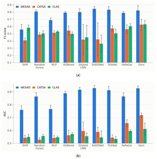
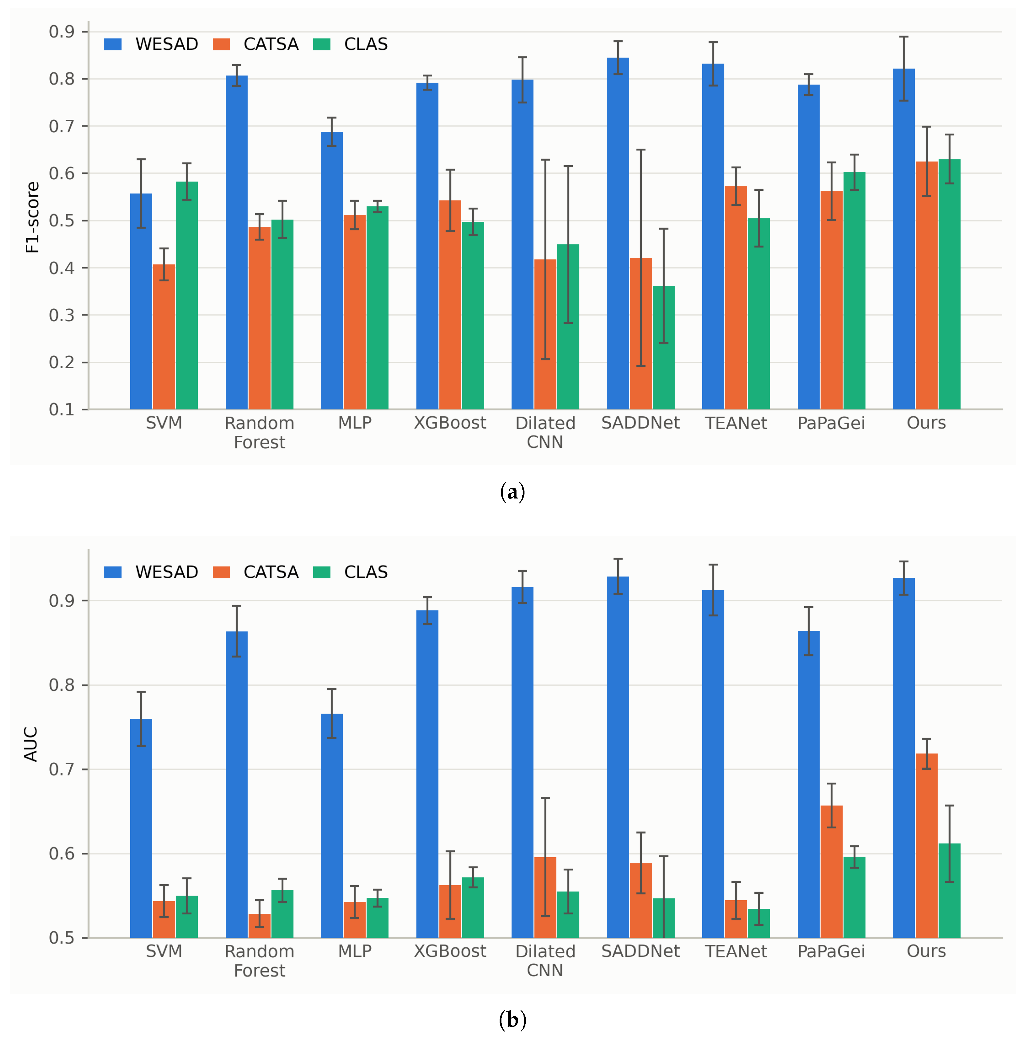
Table 2 and Figure 3 report the F1-score and AUC of all methods on WESAD, CATSA, and CLAS under strict subject-independent 5-fold cross-validation.
Table 2.
F1-score and AUC comparison across all methods (5-fold CV, mean ± std). Best result in each column is shown in bold.
Figure 3.
F1-score and AUC comparison of all methods on WESAD, CATSA, and CLAS under strict subject-independent 5-fold cross-validation. Error bars denote the standard deviation across the five folds. (a) F1-score comparison. (b) AUC comparison.
Averaged across the three datasets, our method attains the best F1-score (0.6919) and AUC (0.7521), outperforming the strongest baseline (PaPaGei) by 4.14 percentage points (pp) in F1-score and 4.67 pp in AUC, and this lead holds across all three datasets rather than resting on any single one.
On WESAD, our F1-score (0.8211) is only slightly below SADDNet’s (0.8443), and our AUC is basically tied (0.9267 vs. 0.9286). On CATSA and CLAS, our method is the best, beating the strongest baseline on each dataset by 5.21 pp and 2.76 pp—whereas SADDNet, the winner on WESAD, drops to 0.4206 and 0.3613 there.
This pattern reflects a systematic difficulty gradient across the three datasets: the TSST protocol used in WESAD elicits a strong, sustained stress response that is easier to separate from rest, whereas the cognitive stressors in CATSA and CLAS induce weaker and less consistent autonomic changes. Our method’s stability at the harder end of this gradient is a direct consequence of its design: the task-adapted pre-trained backbone and the personalized routing prior jointly supply an inductive bias that is comparatively insensitive to the induction protocol and recording device. Additional evaluation metrics, including accuracy, sensitivity, specificity, precision, and calibration, are reported in Appendix D.
4.2. Ablation Studies
To validate the contribution of each core component, systematic ablation experiments were conducted across all three datasets. Five variants are evaluated against the full model (, , all auxiliary losses enabled): (1) w/o PER: single LSTM () without expert routing; (2) frozen backbone: backbone weights frozen during fine-tuning; (3) w/o pre-training: random initialization, no VitalDB pre-training; (4) w/o personalized gate: , pure model-based routing; (5) w/o auxiliary loss: all set to zero, focal loss only. The sensitivity to the expert count K is analyzed separately in Appendix E. Results are summarized in Table 3.
Table 3.
Component ablation results (5-fold CV, F1-score averaged over the three datasets; is the drop in average F1-score relative to the full model).
The ablation results (Table 3) reveal a clear split between two groups of components. The representation-related components—VitalDB pre-training, the auxiliary losses, and end-to-end fine-tuning—dominate the total gain, with each removal lowering F1-score by roughly 3–4 pp; this indicates that the quality of the learned PPG representations, rather than the routing mechanism itself, is the primary bottleneck for short-term stress detection. The routing-related components—the PER expert ensemble and the personalized gate—contribute smaller but still consistent gains, confirming that every component is complementary and none is redundant. The personalized gate’s modest average contribution is strongly dataset-dependent, a point examined in Section 5.
5. Discussion
Contribution of personalized gating. The personalized prior provides a modest gain on average: removing it in favor of pure model-based routing () lowers the average F1-score from 0.6919 to 0.6828, a drop of 0.91 pp. Notably, this gain scales with the number of subjects in each dataset: personalization improves the larger CATSA (50 subjects) and CLAS (59 subjects) cohorts, whereas on WESAD—whose 15 subjects are too few to estimate a reliable personalized prior—dropping the personalized gate raises F1-score from 0.8211 to 0.8578 ± 0.0261. The modest average gain therefore reflects the small subject pool rather than an inherently weak contribution.
Enrollment duration. The personalized prior is extracted from an initial resting-state enrollment segment, for which we used 2 min in the main experiments. As reported in Table A12, shortening this segment to 30 or 60 s changes the average performance only marginally, indicating that the personalization does not critically depend on a long, clean resting recording. For practical wearable deployment, the 2 min resting features could instead be obtained by averaging several short resting segments collected opportunistically during everyday use, or through a brief guided calibration performed at first use, thereby relaxing the requirement for a single continuous 2 min recording.
Pre-training domain gap. VitalDB consists of intraoperative PPG recordings from patients under general anesthesia—a state characterized by depressed autonomic tone, drug-induced heart rate modulation, and mechanical ventilation—which differs substantially from the awake stress responses in WESAD, CATSA, and CLAS. Despite this domain gap, the pre-trained representations transfer effectively to the cognitively oriented datasets: removing VitalDB pre-training degrades F1-score by 9.08 pp on CATSA and 6.20 pp on CLAS. On WESAD, whose strong TSST response can already be learned from scratch, the randomly initialized backbone performs slightly better (2.95 pp). The fact that pre-training is most beneficial on the cognitively oriented datasets suggests that the ten interpretable PPG features capture universal aspects of pulse morphology and beat-to-beat dynamics that are invariant to the anesthesia–awake distinction, and that these representations are especially valuable when stress-induced physiological changes are subtle and hence harder to learn from scratch. The TSST evokes a strong, sustained sympathetic response whose pulse signatures are already prominent in the raw signal, so the pre-trained features offer little additional benefit; the milder autonomic responses to cognitive stressors, by contrast, are subtle, and here the pre-trained features—which encode fine beat-to-beat and morphological dynamics—provide a useful physiological prior. Notably, the apparent drop on WESAD is within the range of random fold-to-fold variation rather than a meaningful negative transfer. Relatedly, the large margin over the frozen PaPaGei probe indicates that generic pre-trained representations alone do not suffice for short-term stress detection and that task-adapted fine-tuning is essential.
Comparison with prior work. The high accuracy figures (up to approximately 98%) reported in prior PPG stress-detection studies should be interpreted with caution. Some of these methods operate on 30 s segments (e.g., TEANet and SADDNet), which contain more physiological information than the 10 s windows used here, and the evaluation protocols also vary: DilatedCNN partitions data at the window level, mixing subjects across training and test sets, while other studies use leave-one-subject-out or do not clearly report their splits. Re-evaluated under our strict subject-independent 5-fold cross-validation on 10 s windows, these baselines attain average F1-scores of only 0.54–0.64, confirming that the apparent performance gap largely reflects these confounds rather than model capability.
Discrimination versus robustness to noise. Beyond the cross-dataset consistency and the subject-scaling of the personalized gate discussed above, the comparison with PaPaGei further indicates that the gains reflect genuine stress discrimination rather than mere noise tolerance: PaPaGei is itself a large-scale pre-trained PPG foundation model with strong noise-robust representations, yet our method still outperforms it by 4.14 pp in average F1-score and 4.67 pp in average AUC—a gap that cannot be attributed to noise handling alone. Moreover, our model attains the lowest average calibration error and competitive sensitivity and specificity (Appendix D and Table A8), showing that its probabilistic outputs, not just its rankings, carry meaningful information about stress.
Hardware differences and resampling. The downstream datasets use different hardware: the Empatica E4 records BVP at 64 Hz at the wrist (WESAD and CATSA), and the Shimmer3 records PPG at 256 Hz at the arm (CLAS). Differences in sensor site, optical path, and sampling rate alter pulse morphology and signal quality, so the same method can perform differently across datasets; we therefore evaluate each dataset separately under subject-independent cross-validation. To obtain a common 125 Hz grid, the 64 Hz signals were upsampled by linear interpolation. This changes the sampling density and can shift detected peaks, perturbing pulse-to-pulse intervals and the derived timing and variability features, but it does not add physiological information.
HRV-style features in pre-training. For each 10 s pre-training window, the two variability features—SDNN (standard deviation of pulse-to-pulse intervals) and RMSSD (root mean square of successive differences)—are computed with standard HRV formulas, but only as HRV-style numerical descriptors of that window. We attach no physiological or clinical meaning of conventional 5 min HRV to them, and no downstream decision relies on such an interpretation. They serve as auxiliary regression targets that encourage the backbone to preserve beat-to-beat and morphological information during stress-label-free pre-training, while keeping the objective aligned with the downstream 10 s window.
6. Conclusions
This study proposes a Personalized Expert Routing (PER) model for short-term wearable PPG-based stress detection. An InceptionTime backbone is pre-trained on VitalDB, a large-scale clinical PPG dataset with zero subject overlap, and we demonstrate that this pre-training improves downstream short-term stress detection. A dual-gating PER module with experts leverages resting-state PPG features as personalized prior knowledge, fusing subject-specific biases with model-based routing to adaptively route samples to specialized LSTM experts without requiring stress labels from new users. Extensive evaluation under strict subject-independent 5-fold cross-validation on WESAD, CATSA, and CLAS demonstrates strong performance (F1-score: 0.8211, 0.6246, and 0.6299, respectively), outperforming the strongest baseline by 4.14 percentage points in average F1-score and 4.67 percentage points in average AUC. Ablation studies confirm the complementary benefits of pre-training, PER architecture, and auxiliary losses—all operating without data leakage. Personalized guidance via resting-state features provides an additional average gain, complementing the pre-trained backbone and the expert routing. A limitation of the current work is that it is a preliminary study, and the pipeline has not yet been adapted to wearable devices: it assumes a 2 min resting-state enrollment segment, has not been profiled for on-device latency or energy consumption, and relies on offline batch processing. Future work will extend pre-training to a domain-matched corpus of awake subjects, profile on-device deployment for low-power wearables, and enable online adaptation of individual profiles for continuous, lifelong stress monitoring.
Author Contributions
Conceptualization, G.G. and Y.R.; methodology, G.G. and Y.R.; software, G.G. and Y.R.; validation, G.G., Y.R., W.W., C.T. and L.W.; formal analysis, G.G. and Y.R.; investigation, G.G., Y.R., W.W. and C.T.; resources, G.G., W.W. and C.T.; data curation, W.W. and C.T.; writing—original draft preparation, G.G. and Y.R.; writing—review and editing, J.C., W.W., C.T. and L.W.; supervision, J.C.; project administration, J.C.; funding acquisition, J.C. All authors have read and agreed to the published version of the manuscript.
Funding
This research was funded by the Natural Science Foundation of Beijing Municipality (grant number L2603041) and the Xiaomi Foundation.
Institutional Review Board Statement
Ethical review and approval were waived for this study because only publicly available, de-identified datasets were used.
Informed Consent Statement
Patient consent was waived because only publicly available, de-identified datasets were used in this study.
Data Availability Statement
All datasets used in this study are publicly available: VitalDB at https://vitaldb.net/dataset/ (accessed on 16 November 2026), WESAD at https://archive.ics.uci.edu/ml/datasets/WESAD (accessed on 16 November 2026), CATSA at https://data.mendeley.com/datasets/g7vbwsxzcy/1 (accessed on 16 November 2026), and CLAS at https://data.mendeley.com/datasets/8hm59ryzb8/1 (accessed on 16 November 2026). The code is available at https://github.com/rongyiming/ppg-per-stress (accessed on 16 November 2026).
Conflicts of Interest
Authors Guosong Gao, Wenlong Wu, and Chunlong Tu were employed by Xiaomi Inc. The remaining authors declare that the research was conducted in the absence of any commercial or financial relationships that could be construed as a potential conflict of interest.
Appendix A. Data Processing Details
Data standardization. Given the discrepancies in acquisition devices and sampling rates across source datasets, all data underwent a uniform preprocessing pipeline. VitalDB was resampled from 500 Hz to 125 Hz and bandpass-filtered; the remaining datasets (WESAD, CATSA, CLAS) were resampled to 125 Hz via linear interpolation (WESAD and CATSA: 64 Hz → 125 Hz; CLAS: 256 Hz → 125 Hz). During training, each extracted 10 s window is further processed with a fourth-order Chebyshev Type I bandpass filter (0.5–4.0 Hz, 0.1 dB passband ripple, zero-phase via forward–backward filtering) to isolate the cardiac frequency band, followed by third-order polynomial detrending to remove baseline wander. No additional manual amplitude normalization is applied; per-sample normalization is handled by an InstanceNorm1d layer inside the model [36].
Signal quality assessment. To objectively validate the data quality before feature extraction, we quantified the signal-to-noise ratio (SNR) of the PPG signals in each dataset as , where is the signal power within the 0.5–4.0 Hz cardiac band and is the remaining out-of-band power. As shown in Table A1, the bandpass filtering consistently increased the SNR by 7.8–12.7 dB across all three datasets, confirming that the filter operates as specified and suppresses out-of-band power. Because this SNR is defined as the ratio of in-band to out-of-band power, the gain should not be interpreted as evidence that in-band motion artifacts have been removed or that classification performance improves.
Table A1.
Signal-to-noise ratio (SNR) of the PPG signals before and after filtering.
Pre-training dataset construction. 10 s segments were randomly sampled via a sliding-window approach from the VitalDB recordings, and the corresponding ten feature labels were computed as regression targets. The resulting dataset was partitioned at the subject level into training and validation sets with a ratio of 85/15, discarding subjects with fewer than 50 segments; the training set optimizes the backbone and the validation set is used for early stopping to prevent overfitting.
Stress-task label mapping. All three datasets are reduced to a binary stress/non-stress label. For WESAD, the TSST phase is labeled stress, while the baseline and amusement phases are labeled non-stress; for CATSA, the three cognitive tasks (Stroop test, logical reasoning, and Sudoku) are labeled stress and the baseline is non-stress; for CLAS, only the Stroop test is labeled stress and the baseline/neutral phase is non-stress, while the remaining states (math test, IQ test, pictures, video clips, and response blocks) are excluded.
Appendix B. Pre-Training Feature Targets
The ten interpretable PPG features used as pre-training regression targets are listed in Table A2.
Table A2.
The ten interpretable PPG features used as pre-training regression targets.
These features are computed from pulse peaks detected on the PPG signal. Because the pulse intervals are derived from PPG rather than ECG, the two heart-rate features are pulse-rate measures, whereas the two HRV indices constitute pulse-rate variability (PRV) measures, used here as surrogates of conventional HRV measures defined on ECG normal-to-normal intervals [26,37]. Because these indices are derived from 10 s windows, they are not clinical HRV measures; conventional HRV analysis is defined on recordings of at least 5 min [26,38], and the rationale, reliability, and limitations of our ultra-short-term choice are discussed in Section 5. In brief, we compute only the time-domain indices SDNN and RMSSD, do not attempt frequency-domain HRV, and use the resulting values as auxiliary regression targets for pre-training rather than as clinical descriptors.
Appendix C. Implementation Details
Software environment. All models were implemented in PyTorch with Python 3.10, and the exact package versions are recorded in the public code repository at https://github.com/rongyiming/ppg-per-stress (accessed on 16 November 2026).
Backbone architecture. The InceptionTime backbone consists of stacked InceptionBlocks, each with a bottleneck layer ( with batch normalization and ReLU), three parallel convolutional branches (kernel sizes 1, 3, and 5), and a max-pooling branch ( followed by ); the four branches are concatenated and fused with a residual connection. Stacking InceptionBlocks with periodic down-sampling constructs a four-level feature pyramid, with channel dimensions of 64, 128, 256, and 512 at levels 0 through 3, respectively. The temporal module consists of parallel single-layer, unidirectional LSTM networks with hidden size 64, each receiving the level-3 (512-dimensional) features as input; input weights use Xavier uniform initialization [39], recurrent weights are orthogonally initialized [40], and all bias terms are zero-initialized except the forget gate bias, which is set to 1 [41].
Pre-training configuration. The level-3 backbone output (512-dimensional) is first projected to 64 dimensions by a linear layer applied to each time step, followed by ReLU and global average pooling over the temporal dimension; the resulting 64-dimensional vector is then mapped to the ten regression targets via a two-layer MLP (64→128→10) with dropout of 0.5, optimized using the mean squared error (MSE) loss. Pre-training uses the Adam optimizer with a learning rate of , a batch size of 512, and a maximum of 100 epochs, with early stopping (patience = 10).
Fine-tuning configuration. The AdamW optimizer [42] is used with a learning rate of for the PER and classification modules and for the pre-trained backbone, a batch size of 128 (with ), and gradient clipping with max_norm = 1.0. Training runs for a maximum of 1000 epochs with early stopping (patience = 50).
Class-imbalance handling. To mitigate class imbalance, an adaptive step size is used during sliding-window extraction: for each subject, a total target window count is computed, where is the subject’s total data length, W is the window length, and is the base step (half the window length at 125 Hz). This target is then split evenly between the stress and non-stress classes ( each), and the per-class step is , where is the subject’s total sample length within that class, ensuring stress and non-stress classes produce approximately equal numbers of windows. Each full experiment (three datasets × five folds) takes approximately 70 min.
Hyperparameter summary. Table A3 summarizes the main hyperparameters of the full model.
Table A3.
Summary of the main hyperparameters.
Computational complexity. The full model contains 2,009,612 parameters (7.67 MiB in 32-bit floating point, fp32) and requires 202,225,464 floating-point operations (FLOPs) for a single 10 s window. On a central processing unit (CPU), the latency is 68–83 ms, corresponding to roughly 120–150× real time. Table A4 summarizes these figures.
Table A4.
Computational complexity of the proposed model.
Appendix D. Additional Evaluation Metrics
In addition to the F1-score and AUC reported in the main text, Table A5, Table A6 and Table A7 report the accuracy, sensitivity, specificity, and precision of all methods under the same strict subject-independent 5-fold cross-validation.
Table A5.
Accuracy comparison across all methods (5-fold CV, mean ± std). Best result in each column is shown in bold.
Table A6.
Average sensitivity and specificity (mean over the three datasets, mean ± std), highlighting the trade-off.
Table A7.
Precision comparison across all methods (5-fold CV, mean ± std). Best result in each column is shown in bold.
Across the four metrics, our method attains the best average accuracy, sensitivity, and precision, together with competitive specificity. Table A6 highlights the sensitivity–specificity trade-off: unlike SADDNet, which achieves the highest specificity (0.7519) but a markedly lower sensitivity (0.5306), our method simultaneously maintains a high sensitivity (0.7215) and a reasonable specificity (0.6536), indicating that it both captures a large fraction of stress events and limits false alarms.
We further assess the calibration of the predicted probabilities using the expected calibration error, computed over ten equal-width probability bins on the pooled five-fold test predictions. Table A8 reports the ECE, and Figure A1 shows the reliability diagrams. ECE is the count-weighted mean absolute difference between the predicted confidence and the observed accuracy over the ten probability bins (lower is better); in the diagrams, the dashed diagonal represents perfect calibration, and larger deviations from it indicate worse calibration.
Figure A1.
Reliability diagrams on the test split with the five-fold predictions pooled. (a) One panel per dataset, comparing the proposed model with the deep learning baselines. (b) One panel per model, with the three datasets overlaid. The dashed diagonal indicates perfect calibration. Curves are drawn only for probability bins with at least of windows, while the reported expected calibration error (ECE) is computed over all ten bins.
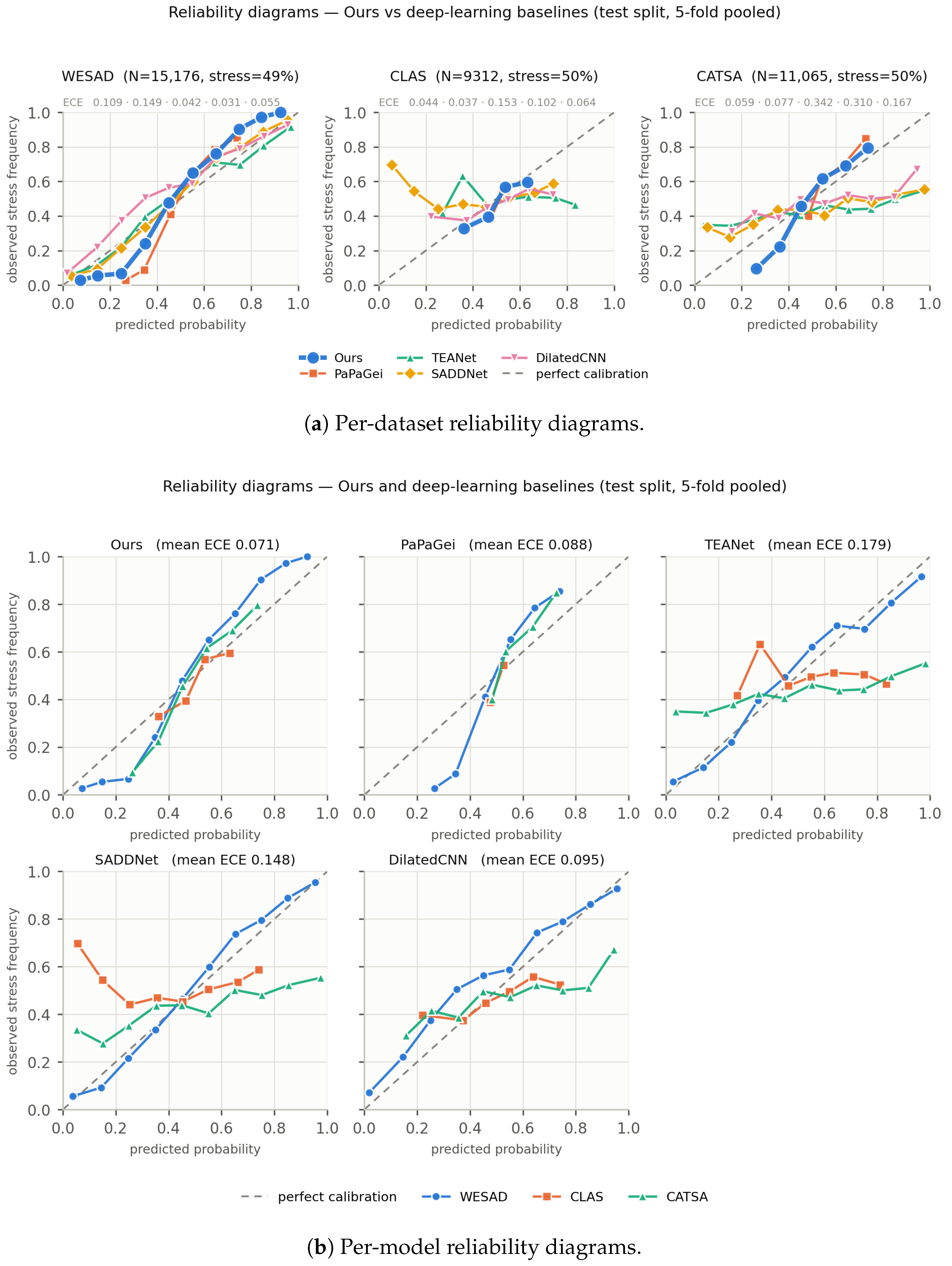
Table A8.
Expected calibration error (ECE) on the test split, computed with the five-fold predictions pooled. Lower is better; the best value in each column is shown in bold.
Our method attains the lowest average ECE of 0.0709 and remains well-calibrated across all three datasets, whereas the baselines degrade substantially on the harder datasets: for instance, TEANet reaches 0.3416 on CATSA. This further supports that the improvements reflect genuine stress discrimination rather than merely noise tolerance.
Appendix E. Supplementary Analyses
Appendix E.1. Temporal Encoder Selection
To justify the choice of recurrent temporal modeling, we compare three encoders—unidirectional LSTM, bidirectional GRU, and Transformer—keeping all other components fixed. Table A9 reports their average F1-score across the three datasets.
Table A9.
Temporal encoder comparison (5-fold CV, F1-score averaged over the three datasets).
The unidirectional LSTM outperforms both the bidirectional GRU (by 1.43 pp) and the Transformer (by 2.59 pp) on average, so we retain the LSTM as the temporal encoder.
Appendix E.2. Sensitivity Analysis of Expert Count K
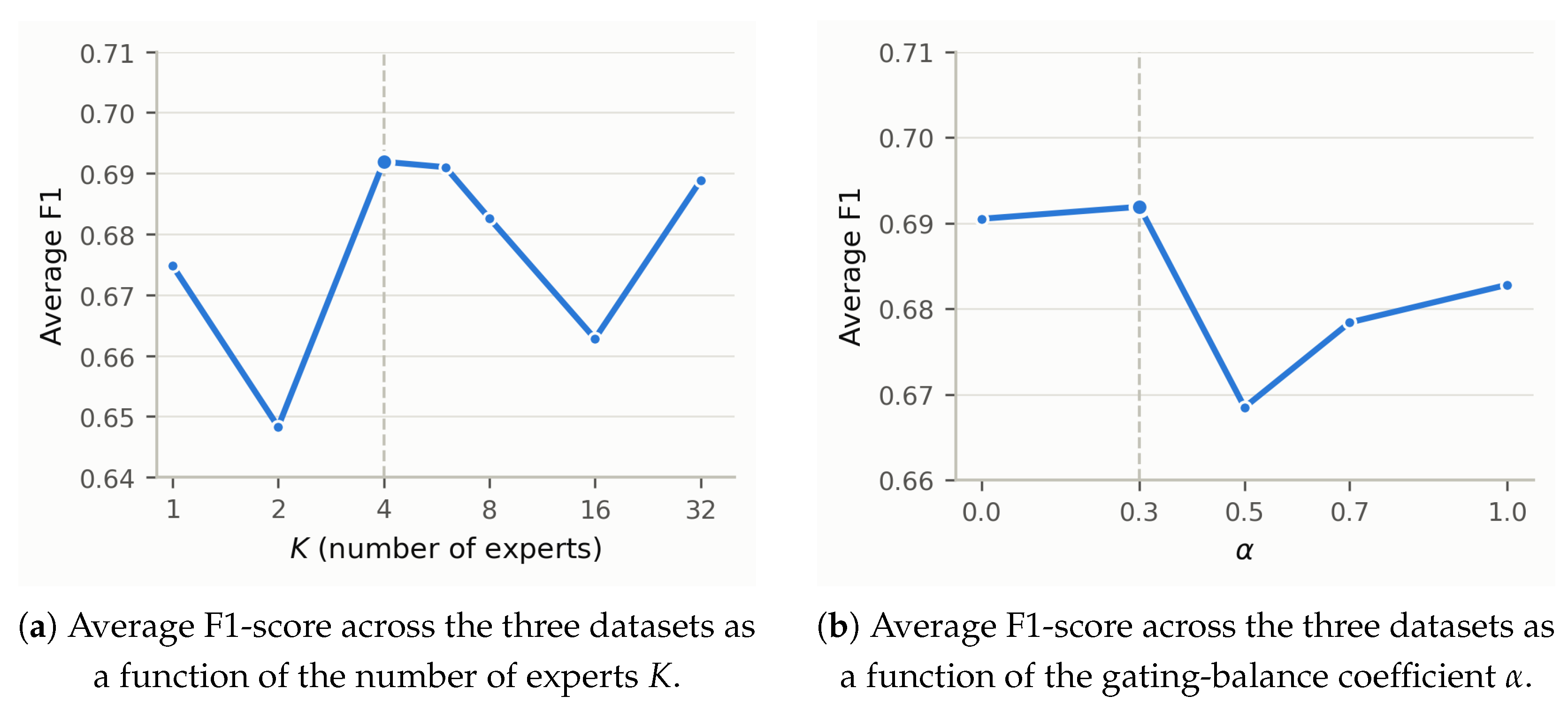
To determine the optimal number of LSTM experts, we vary K from 1 to 32 while keeping all other components fixed at the full configuration. Table A10 and Figure A2 report the F1-score across all three datasets.
Table A10.
Expert-count ablation (5-fold CV, F1-score averaged over the three datasets).
attains the best average F1-score (0.6919), with essentially tied (0.6910). Smaller () and larger () configurations degrade on average, and shows unstable per-dataset behavior. We therefore keep as the default number of experts.
Figure A2.
Sensitivity of the proposed method to the number of experts K (a) and to the gating-balance coefficient (b), under strict subject-independent 5-fold cross-validation.
Appendix E.3. Sensitivity Analysis of α
The gating-balance coefficient controls the balance between the personalized pathway and the model pathway. Table A11 and Figure A2 report an ablation over under the full configuration (, dual-gating, both auxiliary losses enabled).
Table A11.
Gating-balance coefficient () ablation (5-fold CV, F1-score averaged over the three datasets).
On the validation set, F1-score is highest at (0.7153) and lies within the fold-to-fold noise (0.7140); on the test set, attains the best average F1-score (0.6919). We retain so that the content pathway provides a small stabilizing signal while the personalized pathway dominates.
Appendix E.4. Enrollment Duration Sensitivity
To assess the robustness of the personalized prior to the length of the resting-state enrollment segment, we varied the enrollment duration among 30 s, 60 s, and 120 s while keeping all other components fixed. Table A12 reports the F1-score and AUC. The performance remains stable across durations: the average F1-score is 0.6805 for 30 s, 0.6923 for 60 s, and 0.6919 for 120 s, while the average AUC remains essentially unchanged at 0.7575 for 30 s, 0.7550 for 60 s, and 0.7521 for 120 s. This indicates that the personalization strategy does not require a long enrollment window. Nonetheless, a longer resting baseline should in principle provide a more stable estimate of the individual feature, so we retain the 2 min enrollment in the main experiments.
Appendix E.5. Gating Source Ablation
To justify the choice of Expert 0 as the gating source, we compared it with the global-average-pooled (GAP) backbone feature and with the mean or concatenation of all expert outputs, under otherwise identical settings. Table A13 reports the F1-score and AUC; Expert 0 attains the best average F1-score of 0.6919, ahead of the concatenation of all experts at 0.6850, the global-average-pooled backbone feature at 0.6750, and the expert-mean at 0.6729, while remaining competitive in AUC. This indicates that routing from a single expert’s hidden state is not only simpler but also at least as effective as the alternative sources, justifying the adopted design.
Table A12.
Enrollment duration sensitivity (5-fold CV, mean ± std). Best result in each column is shown in bold.
Table A13.
Gating source ablation (5-fold CV, mean ± std). Best result in each column is shown in bold.
References
- World Health Organization. Stress; World Health Organization: Geneva, Switzerland, 2023. [Google Scholar]
- Cohen, S.; Janicki-Deverts, D.; Miller, G.E. Psychological Stress and Disease. JAMA 2007, 298, 1685–1687. [Google Scholar] [CrossRef] [Scilit] [PubMed]
- Poria, S.; Cambria, E.; Bajpai, R.; Hussain, A. A Review of Affective Computing: From Unimodal Analysis to Multimodal Fusion. Inf. Fusion 2017, 37, 98–125. [Google Scholar] [CrossRef] [Scilit]
- Giannakakis, G.; Grigoriadis, D.; Giannakaki, K.; Simantiraki, O.; Roniotis, A.; Tsiknakis, M. Review on Psychological Stress Detection Using Biosignals. IEEE Trans. Affect. Comput. 2022, 13, 440–460. [Google Scholar] [CrossRef] [Scilit]
- Ali, M.S.; Motin, M.A.; Bipro, S.S.; Kabir, S.; Syfullah, M.K.; Kumar, D.K. Detection of Mental Stress From Photoplethysmography for Under-Resourced Healthcare Systems. IEEE Sens. J. 2026, 26, 6293–6301. [Google Scholar] [CrossRef] [Scilit]
- Ali, M.S.; Bipro, S.S.; Motin, M.A.; Kabir, S.; Sharma, M.; Chowdhury, M.E. TEANet: A transpose-enhanced autoencoder network for wearable stress monitoring. arXiv 2025. [Google Scholar] [CrossRef] [Scilit]
- Motaman, K.; Alipour, K.; Tarvirdizadeh, B.; Ghamari, M. A Dilated CNN-Based Model for Stress Detection Using Raw PPG Signals. IET Wirel. Sens. Syst. 2025, 15, e70004. [Google Scholar] [CrossRef] [Scilit]
- Pillai, A.; Spathis, D.; Kawsar, F.; Malekzadeh, M. PaPaGei: Open Foundation Models for Optical Physiological Signals. In Proceedings of the 13th International Conference on Learning Representations (ICLR), Singapore, 24–28 April 2025. [Google Scholar]
- Nie, G.; Fang, X.; Tang, G.; Xiao, Y.; Li, J.; Liu, B.; Li, H.; Hong, S. AnyPPG: An ECG-Guided PPG Foundation Model Trained on Over 100,000 Hours of Recordings for Holistic Health Profiling. arXiv 2025. [Google Scholar] [CrossRef] [Scilit]
- Abbaspourazad, S.; Elachqar, O.; Miller, A.C.; Emrani, S.; Nallasamy, U.; Shapiro, I. Large-Scale Training of Foundation Models for Wearable Biosignals. In Proceedings of the 12th International Conference on Learning Representations (ICLR), Vienna, Austria, 7–11 May 2024. [Google Scholar]
- Ding, C.; Guo, Z.; Chen, Z.; Lee, R.J.; Rudin, C.; Hu, X. SiamQuality: A ConvNet-Based Foundation Model for Photoplethysmography Signals. Physiol. Meas. 2024, 45, 085004. [Google Scholar] [CrossRef] [Scilit] [PubMed]
- Yaseen, E.S.; Şahin, S. Masked Signal Modeling with Self-Supervised Transformers for Stress and Affect Detection Using Wearable Biosignals. Biomed. Signal Process. Control 2026, 118, 109607. [Google Scholar] [CrossRef] [Scilit]
- Schmidt, P.; Reiss, A.; Duerichen, R.; Marberger, C.; Laerhoven, K.V. Introducing wesad, a multimodal dataset for wearable stress and affect detection. In Proceedings of the 20th ACM International Conference on Multimodal Interaction (ICMI); Association for Computing Machinery (ACM): New York, NY, USA, 2018; pp. 400–408. [Google Scholar]
- Motin, M.A.; Ali, M.S.; Bipro, S.S.; Nuha, M.J.; Hasan, A.; Kabir, S. A multi-modal wearable dataset for cognitive attention and task-based stress analysis. Data Brief 2025, 63, 112295. [Google Scholar] [CrossRef] [Scilit] [PubMed]
- Markova, V.; Ganchev, T.; Kalinkov, K. CLAS: A Database for Cognitive Load, Affect and Stress Recognition. In Proceedings of the 2019 International Conference on Biomedical Innovations and Applications (BIA); IEEE: New York, NY, USA, 2019; pp. 1–4. [Google Scholar] [CrossRef] [Scilit]
- Healey, J.; Picard, R. Detecting stress during real-world driving tasks using physiological sensors. IEEE Trans. Intell. Transp. Syst. 2005, 6, 156–166. [Google Scholar] [CrossRef] [Scilit]
- Ghosh, S.; Kim, S.; Ijaz, M.F.; Singh, P.K.; Mahmud, M. Classification of Mental Stress from Wearable Physiological Sensors Using Image-Encoding-Based Deep Neural Network. Biosensors 2022, 12, 1153. [Google Scholar] [CrossRef] [Scilit] [PubMed]
- Ali, M.S.; Motin, M.A.; Kabir, S. ReTeNet: A residual encoder and transformer encoders network for stress monitoring from wearable device. IEEE Signal Process. Lett. 2025, 32, 3635–3639. [Google Scholar] [CrossRef] [Scilit]
- Zhao, L.; Niu, X.; Wang, L.; Niu, J.; Zhu, X.; Dai, Z. Stress Detection via Multimodal Multitemporal-Scale Fusion: A Hybrid of Deep Learning and Handcrafted Feature Approach. IEEE Sens. J. 2023, 23, 27817–27827. [Google Scholar] [CrossRef] [Scilit]
- Rashid, N.; Chen, L.; Dautta, M.; Jimenez, A.; Tseng, P.; Faruque, M.A.A. Feature augmented hybrid CNN for stress recognition using wrist-based photoplethysmography sensor. In Proceedings of the 43rd Annual International Conference of the IEEE Engineering in Medicine and Biology Society (EMBC); IEEE: New York, NY, USA, 2021; pp. 2374–2377. [Google Scholar]
- Rashid, N.; Mortlock, T.; Faruque, M.A.A. Stress detection using context-aware sensor fusion from wearable devices. IEEE Internet Things J. 2023, 10, 14114–14127. [Google Scholar] [CrossRef] [Scilit]
- Koteska, B.; Bogdanova, A.M.; Mitrova, H.; Sidorenko, M.; Lehocki, F. A Deep Learning Approach to Estimate SpO2 from PPG Signals. In Proceedings of the Proceedings of the 9th International Conference on Bioinformatics Research and Applications (ICBRA); ACM: New York, NY, USA, 2022; pp. 142–148. [Google Scholar] [CrossRef] [Scilit]
- Wang, W.; Mohseni, P.; Kilgore, K.L.; Najafizadeh, L. PulseDB: A Large, Cleaned Dataset Based on MIMIC-III and VitalDB for Benchmarking Cuff-less Blood Pressure Estimation Methods. Front. Digit. Health 2022, 4, 1090854. [Google Scholar] [CrossRef] [Scilit] [PubMed]
- Lee, H.C.; Park, Y.; Yoon, S.B.; Yang, S.M.; Park, D.; Jung, C.W. VitalDB, a high-fidelity multi-parameter vital signs database in surgical patients. Sci. Data 2022, 9, 279. [Google Scholar] [CrossRef] [Scilit] [PubMed]
- Fawaz, H.I.; Lucas, B.; Forestier, G.; Pelletier, C.; Schmidt, D.F.; Weber, J.; Webb, G.I.; Idoumghar, L.; Muller, P.A.; Petitjean, F. InceptionTime: Finding AlexNet for Time Series Classification. Data Min. Knowl. Discov. 2020, 34, 1936–1962. [Google Scholar] [CrossRef] [Scilit]
- Task Force of the European Society of Cardiology and the North American Society of Pacing and Electrophysiology. Heart rate variability: Standards of measurement, physiological interpretation and clinical use. Circulation 1996, 93, 1043–1065. [Google Scholar] [PubMed]
- Allen, J. Photoplethysmography and its application in clinical physiological measurement. Physiol. Meas. 2007, 28, R1–R39. [Google Scholar] [CrossRef] [Scilit] [PubMed]
- Jacobs, R.A.; Jordan, M.I.; Nowlan, S.J.; Hinton, G.E. Adaptive mixtures of local experts. Neural Comput. 1991, 3, 79–87. [Google Scholar] [CrossRef] [Scilit] [PubMed]
- Lin, T.Y.; Goyal, P.; Girshick, R.; He, K.; Dollár, P. Focal Loss for Dense Object Detection. In Proceedings of the IEEE International Conference on Computer Vision (ICCV); IEEE: New York, NY, USA, 2017; pp. 2980–2988. [Google Scholar] [CrossRef] [Scilit]
- Kirschbaum, C.; Pirke, K.M.; Hellhammer, D.H. The ’Trier Social Stress Test’—A tool for investigating psychobiological stress responses in a laboratory setting. Neuropsychobiology 1993, 28, 76–81. [Google Scholar] [CrossRef] [Scilit] [PubMed]
- Stroop, J.R. Studies of interference in serial verbal reactions. J. Exp. Psychol. 1935, 18, 643–662. [Google Scholar] [CrossRef] [Scilit]
- Cortes, C.; Vapnik, V. Support-vector networks. Mach. Learn. 1995, 20, 273–297. [Google Scholar] [CrossRef] [Scilit]
- Breiman, L. Random forests. Mach. Learn. 2001, 45, 5–32. [Google Scholar] [CrossRef] [Scilit]
- Rumelhart, D.E.; Hinton, G.E.; Williams, R.J. Learning representations by back-propagating errors. Nature 1986, 323, 533–536. [Google Scholar] [CrossRef] [Scilit]
- Chen, T.; Guestrin, C. XGBoost: A scalable tree boosting system. In Proceedings of the 22nd ACM SIGKDD International Conference on Knowledge Discovery and Data Mining; Association for Computing Machinery (ACM): New York, NY, USA, 2016; pp. 785–794. [Google Scholar]
- Ulyanov, D.; Vedaldi, A.; Lempitsky, V. Instance Normalization: The Missing Ingredient for Fast Stylization. arXiv 2016, arXiv:1607.08022. [Google Scholar]
- Elgendi, M. On the Analysis of Fingertip Photoplethysmogram Signals. Curr. Cardiol. Rev. 2012, 8, 14–25. [Google Scholar] [CrossRef] [Scilit] [PubMed]
- Shaffer, F.; Ginsberg, J.P. An Overview of Heart Rate Variability Metrics and Norms. Front. Public Health 2017, 5, 258. [Google Scholar] [CrossRef] [Scilit] [PubMed]
- Glorot, X.; Bengio, Y. Understanding the difficulty of training deep feedforward neural networks. In Proceedings of the 13th International Conference on Artificial Intelligence and Statistics (AISTATS); PMLR: New York, NY, USA, 2010; pp. 249–256. [Google Scholar]
- Saxe, A.M.; McClelland, J.L.; Ganguli, S. Exact solutions to the nonlinear dynamics of learning in deep linear neural networks. In Proceedings of the International Conference on Learning Representations (ICLR), Banff, AB, Canada, 14–16 April 2014. [Google Scholar]
- Gers, F.A.; Schmidhuber, J.; Cummins, F. Learning to forget: Continual prediction with LSTM. Neural Comput. 2000, 12, 2451–2471. [Google Scholar] [CrossRef] [Scilit] [PubMed]
- Loshchilov, I.; Hutter, F. Decoupled Weight Decay Regularization. In Proceedings of the International Conference on Learning Representations (ICLR), New Orleans, LA, USA, 6–9 May 2019. [Google Scholar]

Disclaimer/Publisher’s Note: The statements, opinions and data contained in all publications are solely those of the individual author(s) and contributor(s) and not of MDPI and/or the editor(s). MDPI and/or the editor(s) disclaim responsibility for any injury to people or property resulting from any ideas, methods, instructions or products referred to in the content. |
© 2026 by the authors. Licensee MDPI, Basel, Switzerland. This article is an open access article distributed under the terms and conditions of the Creative Commons Attribution (CC BY) license.