


Abstract
The rapid growth of Internet of Things (IoT) technology has accelerated its adoption in industrial environments, generating large volumes of both normal and abnormal sensor data. Detecting anomalies in Industrial Internet of Things (IIoT) systems is essential for maintaining industrial sustainability, operational performance, and security. However, the dynamic and real-time nature of IIoT sensor data makes anomaly detection particularly challenging. This paper presents RuleSense, an efficient rule-based anomaly detection framework for IIoT environments. RuleSense is positioned as a lightweight data-intensive monitoring framework that combines edge-cloud processing, interpretable rule-based detection, and joint network-sensor analysis within a realistic IIoT evaluation setting. The design aims to enable early anomaly detection at the edge and suits environments with unreliable internet connectivity, since detection is performed at the edge without depending entirely on cloud processing. By profiling normal device behavior, the attack detection module (RADM) identifies a range of anomalies without a training phase and without attack data for profile construction or detection; its feature subset, weights and thresholds are fixed design-time parameters that were chosen with labeled data. On a held-out test set of the IIoT testbed, RADM achieves 98.54% accuracy and a 98.82% F1-score, and on three external IoT datasets it achieves accuracies between 94.28% and 98.92% with the same parameters. RADM does not reach the accuracy of the strongest supervised models trained on all available features, but it is significantly more accurate than four supervised baselines (XGBoost, Random Forest, Decision Tree and CNN) trained on the same 15 features. When attack classification is needed, the attack classification module (GADM) uses attack profiles constructed from observed attack data to identify specific threat types, achieving 93% attack classification accuracy, evaluated on the earlier attack split and not repeated on the new split. To the best of our knowledge, RuleSense is among the few rule-based intrusion and anomaly detection frameworks for IIoT that combine both network and sensor data to detect a broad range of network threats and data anomalies.
1. Introduction
The Internet of Things (IoT) has become a key enabler of digital transformation in industrial sectors by interconnecting devices and generating large volumes of heterogeneous data, including both normal operational measurements and abnormal events [1]. The Industrial Internet of Things (IIoT), as an industrial extension of IoT, improves automation, efficiency, and decision-making across domains such as manufacturing, energy, healthcare, transportation, and agriculture [2,3]. In these settings, anomaly detection is essential for maintaining safe and efficient operations and for preventing failures and security incidents [4,5].
Intrusion and anomaly detection methods are commonly grouped into supervised, unsupervised, and rule-based approaches [1]. Supervised methods depend on labeled data to train classifiers such as SVM and Random Forest, but often require costly data preparation and may struggle with imbalanced or evolving attack patterns [6]. Unsupervised methods avoid labeled data, yet they may offer lower accuracy and reduced interpretability [7]. Rule-based methods provide low computational cost and clear decision logic, although their ability to adapt to new threats is often limited [8]. In this context, RuleSense adopts a lightweight rule-based strategy that combines network and sensor data to detect both anomalies and intrusions in real time, while avoiding the training overhead of machine learning-based solutions.
Real-time anomaly detection in IIoT remains difficult because sensor streams are dynamic, heterogeneous, and continuously evolving [2]. Many existing studies consider either network traffic or sensor data in isolation [9], which limits their ability to capture the interdependent behavior of industrial environments. In practice, multiple sensors operate simultaneously and produce continuous streams that require timely and coordinated analysis [3].
To address these limitations, this paper proposes RuleSense, a rule-based anomaly detection framework that integrates network and sensor data within a three-layer architecture spanning the perception, edge, and cloud layers. Unlike existing rule-based approaches that rely on manually crafted signatures confined to network-layer inspection [10,11,12], and lightweight ML-based methods that still require labeled training data and degrade under distributional shift [13,14], The attack detection component of RuleSense, RADM, eliminates the need for a training phase by deriving detection boundaries directly from benign device behavior observations, requiring no prior attack data for profile construction or detection. The 15 features were selected with a genetic algorithm and mutual information, the feature weights were set experimentally, and the threshold multipliers cover the value ranges of the features; all of these are fixed at design time and were applied unchanged to the external datasets. The attack classification component, GADM, complements this by constructing attack profiles from observed attack data to identify specific threat types once an anomaly is detected. It jointly analyzes network traffic and sensor measurements, enabling detection of both process-level anomalies and communication-layer intrusions within a single unified framework, while remaining effective under unbalanced data conditions. Early detection at the edge layer reduces latency and bandwidth consumption, and supports continuous local operation in environments with limited connectivity. To evaluate the approach, we developed a realistic IIoT testbed equipped with diverse industrial sensors for synchronized multimodal data collection.
The main contributions of this paper are as follows:
- We propose RuleSense, a three-layer edge-cloud anomaly detection framework for IIoT that supports low-latency, distributed analysis without a training phase.
- We introduce a lightweight training-free attack detection algorithm (RADM) that models device-specific benign behavior and identifies deviations in real time without requiring prior attack knowledge or labeled training data, and a complementary attack classification module (GADM) that identifies specific attack types using behavioral deviation profiles.
- We design a unified detection framework that jointly analyzes network traffic and sensor data, enabling simultaneous detection of communication-layer intrusions and process-level anomalies.
- We implement and evaluate the framework on a realistic IIoT testbed with heterogeneous devices, and validate it further on a publicly available benchmark dataset.
In the remainder of this paper, Section 2 reviews existing studies on IIoT anomaly detection. Section 3 presents the proposed three-layer edge architecture together with the profiling and detection algorithms that enable anomaly detection from both network and sensor data perspectives. Section 4 describes the IIoT testbed and implementation details of the proposed framework. Section 5 reports the experimental evaluation. Section 6 discusses the limitations of the current study. Finally, Section 7 concludes the paper and outlines directions for future research.
2. Related Work
The increasing adoption of IIoT has expanded the attack surface of industrial systems and intensified the need for effective anomaly and intrusion detection. Existing studies differ mainly in detection strategy, monitored data type, and evaluation setting, with comparatively limited attention given to lightweight rule-based methods that jointly analyze network and sensor data in real time.
2.1. Signature-Based and Anomaly-Based Detection
Signature-based methods detect attacks by matching observed behavior against known patterns. They are effective for known threats but require frequent updates and struggle with evolving attacks [5]. Hybrid designs such as AS-IDS [15] and the multi-layered framework of Zhang et al. [16] combine both strategies to partially address this limitation. Bhardwaj et al. [17] further proposed the CTI algorithm to identify concealed attack processes in ICS logs.
Anomaly-based methods detect deviations from normal behavior and are better suited to novel threats, but often produce higher false positive rates and depend on accurate behavioral modeling [3]. Representative examples include ASTREAM [18], which combines sliding windows and LSHiForest for scalable streaming detection, EATU [19], which pairs autoencoders with model explanation, and the federated reinforcement learning approach of Wang et al. [20]. The outlier-scoring framework of Kreimel et al. [21] also illustrates the flexibility of anomaly-based detection, though often at the cost of interpretability.
2.2. Learning-Based Detection
Classical ML models such as SVM, KNN, and Random Forest have been widely applied to industrial cybersecurity tasks [4,22,23,24]. Deep learning has extended this further through CNN-, autoencoder-, and hybrid architectures that improve classification under class imbalance and large-scale traffic [25,26,27]. Federated learning has been explored to support privacy-preserving distributed detection [28,29], while time-series and graph-based models capture temporal dependencies and structural relationships in industrial data [30,31,32,33,34]. Despite strong performance, these approaches typically require labeled data, feature engineering, and retraining, introducing overhead that limits practicality in resource-constrained deployments.
2.3. Data Modality and Rule-Based Methods
Many studies focus exclusively on network traffic [22,32,35,36] or sensor measurements [18,19,30,33,37], while joint analysis of both remains uncommon [38,39,40]. This separation limits detection scope in environments where attacks affect both communication patterns and physical process variables.
Rule-based methods offer interpretability, low computational cost, and real-time suitability, yet remain underexplored in IIoT. Traditional rule-based IDS has been studied broadly [10,11,12,41,42], but IIoT-specific applications are limited. Zhu et al. [43] applied association rule mining for ICS anomaly detection on SWaT and WADI, Mehmood et al. [13] combined fuzzy logic with ML classifiers for IoT intrusion detection, and recent work has explored rule extraction from learning models for explainability [44,45,46]. These approaches, however, focus on either sensor or network data alone, or rely on heavyweight learning components during rule generation. Lightweight, training-free frameworks for joint network-sensor detection in IIoT remain limited.
2.4. Evaluation Settings and Research Gap
Most existing studies are evaluated on public datasets such as NSL-KDD, TON-IoT, Edge-IIoT, SWaT, and WADI [47,48,49,50,51], which do not always reflect the operational constraints of real deployments. Table 1 compares representative studies across method type, monitored data, training requirement, and edge or real-time support. Unlike prior work, RuleSense combines network and sensor data within a training-free rule-based framework evaluated in a real-time testbed setting.
Table 1.
Representative IIoT anomaly detection studies compared along dimensions most relevant to RuleSense.
Table 1 compares representative studies using the criteria most relevant to our framework, including method type, monitored data, training requirement, evaluation setting, and edge or real-time support. Unlike most prior studies, RuleSense combines network and sensor data within a training-free rule-based framework and is evaluated in a real-time testbed setting.
3. Methodology
This section presents the RuleSense architecture, its workflow, and the profiling and detection algorithms.
3.1. Dynamic Rule-Based Approach
Unlike conventional rule-based systems that rely on manually defined rules, the proposed approach automatically derives interpretable, device-specific rules from a predefined feature set. This enables adaptive and transparent decision-making tailored to the operational profile of each device. In contrast to clustering-based methods, which group observations by similarity without explicit decision logic, RuleSense produces structured rules that directly represent device behavior.
The rule generation process is designed for noisy industrial environments, where sensor errors, communication interruptions, and transient fluctuations are common. By emphasizing persistent behavioral patterns rather than isolated deviations, the framework improves the reliability of anomaly detection. It also supports incremental class expansion, allowing new device behaviors or operating states, such as those introduced by firmware updates or reconfiguration, to be incorporated without retraining. This property improves scalability and makes the framework suitable for evolving IIoT deployments.
As shown in Figure 1, the proposed mechanism follows a multi-phase architecture for anomaly detection and classification in IIoT networks. The process begins with device profiling, where real-time device data is used to model normal behavior. These profiles are then used to generate device-specific rules for the Rule-based Anomaly Detection Module (RADM), a lightweight edge-deployable component designed for low-latency detection with minimal computational overhead.
Figure 1.
Mechanism Overview.
In parallel, anomalous observations are analyzed through an attack profiling process to extract characteristic attack patterns. These patterns are correlated with device profiles to derive attack-specific rules used by the Global Anomaly Detection Module (GADM) for attack classification. In contrast to RADM, GADM operates in the cloud and uses greater computational resources to support more precise classification. This division enables efficient anomaly detection at the edge while preserving detailed attack analysis in the cloud, thereby improving both responsiveness and accuracy in IIoT security.
3.2. Framework Architecture
Figure 2 presents the overall architecture of RuleSense, which follows a hybrid three-layer design consisting of the Perception, Edge, and Cloud layers. Each layer performs a distinct role in the anomaly detection pipeline.
Figure 2.
Rulesense Framework Architecture Overview.
- Perception Layer: This layer interfaces with the physical environment through sensors that collect measurements such as temperature, humidity, and motion. Sensor data is transmitted to the edge layer via MQTT, a lightweight publish-subscribe messaging protocol widely adopted in IIoT environments for its low bandwidth overhead and support for unreliable networks. The MQTT broker, hosted at the edge layer, acts as the central communication hub between perception-layer devices and the data collection module. While MQTT provides efficient and reliable data transmission, its broker-centric architecture introduces a potential single point of failure and a security-sensitive integration point. Unauthorized access to the broker or injection of malicious messages during the profiling phase represents a known attack vector, including profile poisoning, which is discussed as a limitation in Section 6. Further implementation details of the MQTT broker are provided in Section 4.2.2.
- Edge Layer: This layer performs real-time processing near the data source and includes two main modules:
- (a)
- Data Collection: Collects sensor and network data and hosts the MQTT broker for efficient data acquisition.
- (b)
- Rule-Based Anomaly Detection: Performs local rule-based analysis to support real-time anomaly detection, alert generation, and responsive edge actions. RADM is specifically designed for edge deployment by minimizing computational and memory requirements. It performs detection by comparing each incoming data slice against a pre-computed device profile across 15 features, with a per-slice detection complexity of where d is the number of monitored features. No matrix operations, model inference, or iterative optimization are required at inference time. The device profiles occupy space where k is the number of monitored devices, remaining constant after the profiling phase and not growing with incoming data volume. These properties make RADM suitable for deployment on hardware such as the Raspberry Pi 4 used in this study. GADM, in contrast, compares deviation vectors against multiple attack profiles and applies weighted scoring across all attack categories, requiring higher memory and computation, and is therefore hosted on the cloud layer where greater resources are available.
- Cloud Layer: This layer provides secure storage, rule extraction, and advanced analysis. Specifically, it hosts the Global Anomaly Detection Module (GADM), which performs attack classification by comparing behavioral deviation vectors against stored attack profiles using weighted scoring across multiple attack categories. This classification process requires comparing an incoming deviation pattern against all known attack profiles simultaneously, which involves higher memory and computational demands than the per-feature threshold comparison performed by RADM at the edge. The cloud layer also supports aggregation of detection events across multiple edge nodes, long-term storage of device and attack profiles, and periodic profile updates to accommodate evolving device behavior.
This architecture enables early anomaly detection at the edge, reducing latency and bandwidth consumption, while offloading more computationally intensive analysis to the cloud. As a result, it improves scalability, efficiency, and overall system responsiveness.
3.3. Framework Workflow Overview
As illustrated in Figure 3, the RuleSense framework operates in four key stages: Data Collection, Data Preparation, Profiling, and Detection, each critical to the system’s accuracy and effectiveness.
Figure 3.
RuleSense Framework Workflow Overview.
In Figure 3, solid lines represent the real-time data flow between components during live detection, while dotted lines indicate the profile write operations through which generated profiles are stored in their respective repositories during the profiling phase.
3.3.1. Data Collection Phase
The Data Collection Module gathers IIoT sensor data via an MQTT broker and network traffic data through a capture module. Operating at the edge, it aggregates these streams into vectors, integrating sensor and network data for comprehensive analysis and anomaly detection.
3.3.2. Data Preparation Phase
The Data Preparation stage consists of three modules: Preprocessing, which removes noise to ensure accuracy; Grouping, which clusters data by device for easier analysis; and Time Slicing, which segments data into fixed time windows to facilitate time-based feature extraction.
3.3.3. Profiling Phase
The Profiling stage is a key component of the proposed method and consists of three main modules:
- Dynamic Feature Extraction: This module dynamically extracts a predefined set of features from each data slice for further analysis. The extracted features span both network-level and application-level data sources, including packet counts, protocol distributions, IP and MAC address sets, inter-arrival intervals, sensor message counts, data type distributions, and sensor data ranges. The complete list of 15 features used in this study is provided in Table 6.
- Profiling: This module constructs and maintains behavioral profiles for both devices and known attacks using extracted features. It consists of three sub-modules:
- –
- Device Profiling: In a controlled, anomaly-free setting (Profiling Mode), the system generates unique behavior profiles for each device, stored in a global repository. During Live Mode, these profiles support real-time detection and classification. Detailed mechanisms are presented in later sections.
- –
- Attack Profiling: Based on testbed attack data, this module captures distinct attack patterns and their effects on device behavior. These pre-generated profiles, stored in the Attack Profile Repository, are continuously used during Live Mode for attack identification.
- –
- Dynamic Profiling: To accommodate evolving device behavior, this sub-module is designed to support periodic profile updates. Incorporating a delay mechanism before applying profile changes is a planned safeguard to reduce the risk of anomaly contamination during updates. Full experimental validation of dynamic profiling and poisoning resistance under adversarial conditions remains a direction for future work.
3.3.4. Detection Phase
This phase comprises two modules: the Rapid Rule-based Anomaly Detection Module (RADM) for edge-level detection using device profiles, and the Global Anomaly Detection Module (GADM) for cloud-based attack classification. Detection and classification are supported by the Device and Attack Profile Repositories. Detailed descriptions are provided in Section 3.5 and Section 3.7.
3.4. Profiling Mechanism
The profiling phase is essential to the proposed framework, generating two profile types: device profiles, capturing normal device behavior, and attack profiles, describing attack characteristics and their impact on device data. The mechanism consists of six steps (Figure 4):
Figure 4.
RuleSense Profiling Mechanism. The six-stage pipeline processes raw IIoT stream data through: (1) stream data ingestion of mixed-device network packets and sensor logs, (2) preprocessing to remove redundant fields, (3) grouping by device or attack type, (4) time slicing into fixed n-second windows, (5) dynamic feature extraction producing per-slice feature vectors, and (6) profile generation using the Device and Attack Profiling Algorithms, storing results in the Device Profile Repository and Attack Profile Repository respectively.
- 1.
- Data Handling: The system processes unordered stream data (network packets and sensor logs).
- 2.
- Preprocessing: Redundant features, such as transport and application layer details, protocol-specific fields, and payload data, are removed to create a concise dataset.
- 3.
- Data Grouping: For device profiling, data is grouped by device (e.g., group contains log and network data for device x). For attack profiling, data is grouped by attack type (e.g., group includes data for all devices targeted by attack x).
- 4.
- Time Slicing: Stream data is divided into fixed time windows for structured analysis.
- 5.
- Dynamic Feature Extraction: Network and log features are extracted from each time slice and stored in feature vectors (e.g., vector in Figure 4. List of features used is provided in Table 6.
- 6.
- Profile Generation: Using the extracted feature vectors, device and attack profiles are created through distinct algorithms tailored to each profiling type. These algorithms are detailed in the next section.
The two generated profiles serve as inputs to distinct detection algorithms. The Device Profiles, which capture the normal behavior of devices, are utilized in the Attack Detection Algorithm to identify deviations indicative of potential attacks. In contrast, the Attack Profiles are employed by the Attack Classification Algorithm to categorize the detected attacks into specific types. The subsequent sections provide detailed descriptions of both algorithms.
3.5. Attack Detection Mechanism
The attack detection mechanism begins with the Device Profiling Algorithm, which models the normal behavior of each device based on observed data patterns. These profiles serve as a baseline for identifying anomalous behavior. Once established, the Attack Detection Algorithm continuously monitors device activity and compares it against the corresponding device profiles. Any significant deviation from the expected behavior is flagged as a potential attack. This approach is entirely rule-based and does not require a training phase, which keeps its computational cost low. Below, we first present the Device Profiling Algorithm in detail, followed by a description of the Attack Detection Algorithm.
3.5.1. Device Profiling Algorithm
The Device Profiling Algorithm captures key characteristics of a device’s normal behavior, enabling the RADM Module to detect anomalies or attacks. In Equations (1) and (2), represents the feature vector for all devices across slices . The distance between values in is then calculated using Equation (3). Numerical features are measured using Manhattan distance, while string features use Jaccard distance to quantify dissimilarity (Equation (4)). The mean values of these distances form the vector , representing distance vectors for device and feature . The profile product is computed using Equation (5), incorporating weighting values to reflect feature importance in detection. Finally, the device profile vector is determined in Equation (6) as a vector of vectors containing profile data for all devices and features, denoted as .
where n is the number of slices, and
3.5.2. Attack Detection Algorithm
The Attack Detection Algorithm leverages the device profiles generated during the profiling phase to identify anomalies and potential attacks. This process is implemented through the Rapid Rule-Based Anomaly Detection Module (RADM), which compares current device behavior against the pre-established normal profiles. RADM operates using a lightweight, rule-based approach, specifically designed for efficient execution on resource-constrained edge devices common in IIoT environments. By eliminating the need for training and enabling local processing, RADM is designed to support real-time detection with reduced dependency on cloud infrastructure. In this section, we detail the Attack Detection Algorithm, focusing on how RADM uses device profiles to identify behavioral deviations indicative of attacks.
The attack detection module comprises two key functions: Attack_detection_module and detect_attack algorithm. As shown in Algorithm 1, the mechanism takes as input the device profiles , data streams , and distance thresholds. It iterates through each data slice in , identifies the device , and extracts its profile . The detect_attack function (Algorithm 2) is then called, using the device profile, data stream, and thresholds. The function calculates the distance between each feature in the test data and the corresponding mean in the device profile. If the distance exceeds the allowed threshold for any feature, it returns true, indicating an attack. If no threshold is exceeded, it returns false. When detect_attack function returns true, the attack_classifier function (Algorithm 3) classifies the attack type using the device profile, data stream, and feature weights.
| Algorithm 1 Attack Detection Module (RADM) |
Require: , , distance_thresholds 1: function Attack_detection_module(, , distance_thresholds) 2: for each slice in do 3: Determine which is the device of this slice 4: Extract which is the profile for Device 5: detect_attack(, , distance_thresholds) 6: if is True then 7: attack_classifier(, , , weighted_scores) 8: end if 9: end for |
As shown in Algorithm 2, RADM compares each feature of the incoming slice against its profile-derived threshold, defined as the maximum observed profile distance multiplied by a feature-specific multiplier. For every feature that exceeds its threshold, a normalized excess, clipped to , is computed. The global score is the weighted average of these excesses over the violating features only, and a slice is flagged as an attack when this score reaches the decision boundary of 0.01. A slice can therefore be flagged only if at least one feature exceeds its threshold by a relative margin of at least 0.01, and when a single feature violates its threshold, exceeding it by this margin is sufficient to flag the slice. In practice, RADM thus behaves essentially as a disjunctive rule over the 15 features. The decision boundary acts as a small tolerance margin that discards negligible excursions, and the feature weights only modulate the score among the violating features. False-alarm control is therefore provided mainly by the per-feature threshold multipliers rather than by agreement across features, which is why the sensitivity analysis in Section 5.12 focuses on these multipliers.
| Algorithm 2 Detect Attack Function |
Require: , , feature_thresholds, feature_weights, attack_threshold 1: function detect_attack(, , feature_thresholds, feature_weights, attack_threshold) 2: 3: 4: for each feature in do 5: 6: 7: if then 8: 9: 10: 11: end if 12: end for 13: if
then 14: 15: else 16: 17: end if 18: return
|
| Algorithm 3 Attack Classification Module (GADM) |
Require: , , , weighted_scores 1: function attack_classifier(, , , weighted_scores) 2: 3: for each feature in do 4: {Step 1: compute deviation of sample from device profile} 5: 6: for each attack profile in do 7: {Step 2: compute distance between deviation and attack profile} 8: 9: end for 10: end for 11: for each attack profile in do 12: {Step 3: compute weighted similarity score per attack profile} 13: 14: end for 15: {Step 4: select top-x candidates by lowest distance, break ties by score} 16: 17: 18: return chosen_att_class |
3.6. Computational Complexity of RuleSense
The time and space complexity of RuleSense is analyzed with respect to the profiling and detection phases separately. During profiling, the algorithm iterates over n time slices, d features, and k devices. For each device–feature pair, it computes pairwise distances across slices and averages them (Equations (3)–(5)), giving a profiling time complexity of . The resulting device profiles store one mean distance and one max distance value per device–feature pair, yielding a space complexity of , which remains constant after profiling is complete and does not grow with incoming data volume.
During detection, RADM (Algorithm 1) processes each incoming slice by computing the distance between the test data and the stored profile mean across all d features (Algorithm 2), giving a per-slice detection complexity of . This makes inference time independent of the number of historical observations and suitable for continuous real-time streaming without accumulating latency.
In contrast, ML-based methods such as Random Forest require training time and storage for t trees, while deep learning models involve iterative backpropagation over multiple epochs with substantially higher memory footprints. These theoretical bounds are consistent with the empirical results in Figure 16, where RuleSense achieves lower CPU time and RAM usage than all compared methods, despite running on a resource-constrained Raspberry Pi edge device rather than a high-performance server.
3.7. Attack Classification Mechanism
The Attack Classification Mechanism is responsible for identifying the specific type of attack once an anomaly has been detected and it begins with the Attack Profiling Algorithm, which constructs attack profiles by capturing the distinguishing characteristics of each attack along with their impact on normal device behavior. This is achieved by executing various attacks and analyzing the resulting deviations from device-specific baseline patterns. While device profiling is used to detect anomalies, attack profiling focuses on identifying and classifying specific attack types.
3.7.1. Attack Profiling Algorithm
Unlike device profiling, attack profiling captures the key characteristics of each attack and its impact on device data while considering normal device behavior. It measures deviations from normal patterns caused by attacks or anomalies. As shown in Equations (7) and (8), represents the vector of all features in extracted for all attacks in across slices . The distance for each value in the attack vector is calculated using Equation (9), measuring the deviation between the attack vector (for each device) and the device profile to assess how the attack alters normal device behavior. As in device profiling, numerical features are analyzed using the Manhattan distance, and string features are evaluated with the Jaccard distance, as specified in Equation (10). The mean distances are then computed using Equation (11), producing the vector , which represents the distance vectors for attack for feature . Like device profiling, the product is determined using Equation (12), applying weighting values to generate a weighting score for the profile . Finally, the attack profile vector is obtained using Equation (13), representing the complete set of profile vectors for each attack and feature. The attack profiling process is performed only once. When a new device joins the network, only its device profile needs to be calculated, and the attack type can be identified using the device profile in Equation (10). These attack profiles are then utilized in the GADM module for attack classification, enabling accurate identification of attack types.
where
3.7.2. Attack Classification Algorithm
The classification process is carried out by the Global Anomaly Detection Module (GADM), which operates in the cloud due to its higher computational demands. GADM compares the features of data flagged by the detection phase against the profiles stored in the Attack Profile Repository to determine the corresponding attack type. Unlike traditional classification methods such as clustering, which typically group attack data into predefined categories without considering their broader context, GADM takes into account both the characteristics of the attack data and their effects on different devices. This is accomplished through a normalization process that quantifies the attack’s impact across various device types, enabling the generation of generalized yet effective attack profiles.
Once the Attack Detection Algorithm identifies an attack, the Attack Classification Algorithm is triggered to determine the specific attack type. The attack_classifier function (Algorithm 3) operates in two stages. In the first stage, the weighted distance between the observed behavioral deviation and each stored attack profile is computed across all features, and the top-x candidate profiles with the smallest mean distance are selected as the closest matches. In the second stage, a weighted similarity score (Equation (14)) is computed for each candidate, where a higher score indicates a closer match. The attack class with the highest similarity score among the top-x candidates is returned as the classification result.
The attack classification score for a candidate attack profile is defined as:
where is the deviation of the incoming sample from the device profile for feature , is the stored attack profile value for attack and feature , is the feature weight, and is a small constant for numerical stability. A higher score indicates a closer match between the observed deviation pattern and the attack profile.
As shown in Algorithm 3, GADM performs attack classification by calculating the distance between each feature in the new data and all attack profiles stored in the Attack Profile Repository. While this rule-based approach is significantly more efficient than traditional machine learning or deep learning methods, it involves comparing against multiple profiles, which increases computational overhead. Due to these higher resource demands, GADM is hosted in the cloud, where it can leverage greater processing capabilities to ensure accurate and scalable attack classification.
4. Testbed and Dataset Implementation
Existing datasets are often limited to network packets or sensor data, lacking sensor type diversity. To address these limitations and evaluate RuleSense, we developed a testbed with various sensors and network devices, enabling the collection of both sensor and network data.
This section details the testbed setup, including the IIoT sensors, system components such as the MQTT broker, and the data collection process. It also covers the Data Generation step and attacker device information.
4.1. Testbed Setup
To support RuleSense, we developed a real IIoT testbed that integrates multiple sensors and network devices to generate authentic sensor and network data. This setup enables real-time data collection and anomaly detection while addressing the limited realism and coverage of many existing IoT and IIoT datasets.
As shown in Figure 5 and Figure 6, the testbed is designed for end-to-end data generation, collection, and analysis. Sensors transmit measurements over WiFi to a local access point connected to a switch that manages network traffic. The edge layer includes an MQTT broker for sensor data collection, a network capture tool for real-time traffic monitoring, and the RADM module for local anomaly detection. The devices listed in Table 2 connect to the Internet through a router, while cloud integration provides additional resources for further analysis. This design supports scalable and realistic evaluation of RuleSense under operational IIoT conditions.
Figure 5.
Testbed Architecture.
Figure 6.
Testbed Deployment.
Table 2.
Testbed Network Devices.
4.2. Implementation
This section summarizes the implementation of the main RuleSense components, including the IIoT sensors, MQTT broker, attacker devices, and cloud infrastructure.
4.2.1. IIoT Sensors
The IIoT testbed consists of 15 Arduino-based devices equipped with sensors commonly used in industrial environments. Each device transmits measurements over WiFi to the MQTT broker using the MQTT protocol, with data published to dedicated topics for efficient management and processing. The specifications of the deployed sensors are listed in Table 3.
Table 3.
Testbed IIoT Sensors.
4.2.2. MQTT Broker
MQTT was adopted for sensor data transmission because of its widespread use and lightweight operation in IIoT environments. All sensors communicate with a local MQTT broker deployed at the edge layer, enabling reliable low-latency data collection while reducing unnecessary internet transmission. This design limits external exposure and helps reduce the risk of data leakage. The implementation uses Eclipse Mosquitto [57], an open-source MQTT broker suitable for resource-constrained devices.
4.2.3. Attacker Devices
As shown in Figure 5, attack traffic was generated using Raspberry Pi devices listed in Table 2. The attack setup comprises nine devices: one Raspberry Pi 4 Model B 8GB acting as the botmaster for reconnaissance, denial-of-service (DoS), and man-in-the-middle (MitM) attacks, and eight Raspberry Pi 4 Model B 2GB devices acting as attacker slaves for distributed denial-of-service (DDoS) attacks.
4.2.4. Cloud Infrastructure
A Dell server, specified in Table 2, serves as the cloud layer. It hosts the message broker, an Elasticsearch cluster for data storage and analysis, and the GADM service for deeper inspection of collected events.
4.3. Dataset and Reproducibility
The dataset used in this study was generated through a realistic IIoT testbed and is referred to as DataSense. DataSense is publicly available through the CIC Dataset portal https://www.unb.ca/cic/datasets/iiot-dataset-2025.html, accessed 16 April 2026. and provides synchronized network-level and application-level (log) data collected under both benign and attack conditions. To further support reproducibility, the dataset is accompanied by associated resources including configuration details, feature descriptions, and supporting materials required to replicate the experimental setup described in this paper.
The testbed was designed to capture realistic operational behavior by integrating heterogeneous devices, including Arduino-based industrial sensors, Raspberry Pi nodes, and network infrastructure components (Table 2 and Table 3). Sensor data was aggregated through an MQTT broker (Eclipse Mosquitto [57]) hosted on a Raspberry Pi, while MQTT logs were collected using Filebeat [58] and stored in an Elasticsearch cluster. In parallel, network traffic was mirrored at the switch and forwarded to a dedicated Kali Linux monitoring node, where continuous packet capture was performed using TShark [59]. All devices were time-synchronized to ensure precise alignment between packet traces and log records.
DataSense contains complete benign traces together with a broad set of controlled attack scenarios, including reconnaissance, denial-of-service, distributed denial-of-service, malware, brute-force, and web-based attacks, executed using dedicated attacker nodes. This dual-perspective collection provides a unified view of device behavior across both network and application layers. The complete extracted feature set is summarized in Table 4, while the lightweight subset used in this study is listed in Table 6. Further details on the testbed design, data generation workflow, feature extraction, and feature selection are provided in the DataSense publication [60].
Table 4.
Complete List of Features in the Dataset.
4.3.1. Benign Data Collection
Benign data was collected over 12 h under normal operating conditions, encompassing typical device activity patterns during and after work hours to reflect realistic and varied device behavior. During this period, devices generated telemetry, control messages, and service traffic across the testbed network. MQTT logs were collected using Filebeat and indexed in Elasticsearch, while mirrored network traffic was captured using TShark. All systems were time-synchronized to maintain alignment between log and packet data.
The benign recording was divided into two temporally separate blocks. The first block, one hour long, is used for model fitting. Five minutes of this block were used to build the device profiles of RuleSense, yielding 1140 profiling slices used exclusively for profile construction. The training sets of the machine and deep learning baselines were drawn from the same block, so that all methods are fitted on essentially the same benign data. The second block, separated from the first by a gap of two hours, is used only for evaluation, and the test sets of all methods are drawn from it. No benign slice used for profiling or training belongs to the evaluation set.
Attack samples follow a stratified 80/20 split into training and test sets. The attack samples reserved for constructing the attack profiles of GADM are excluded from the training sets of all machine and deep learning models. Table 5 summarizes the collected data and the train and test composition used in the experiments, while Table 4 and Table 6 report the complete and selected feature sets.
Table 5.
IIoT Data Collection and Train/Test Split Summary. The upper block lists the total data collected; the lower block lists the slices used in the experiments of this paper.
Table 6.
Selected List of Features Utilized in the proposed approach.
4.3.2. Attack Data Collection
To evaluate the proposed system, diverse attacks were launched against the main IIoT testbed components, including sensors, the MQTT broker, network infrastructure, and edge devices. As described in Section 4.2.3, nine Raspberry Pi-based attacker nodes were used, with each attack executed for one minute against a designated target while network and log data were collected from the entire testbed.
More than 46 attacks were conducted, covering DoS, DDoS, reconnaissance, brute-force, malware, and web-based threats. The collected data was segmented into 10-s slices with a 5-s stride. The overlap was intentionally applied to attack data to increase the number of evaluation samples per attack type, since each attack session lasts one minute and produces only six non-overlapping slices, which is insufficient for reliable per-attack evaluation across 46 attack categories. Benign data, collected over a continuous 12-h session, produces sufficient samples without overlap and was therefore sliced without stride. We acknowledge that the overlapping attack windows introduce partial dependence between adjacent samples, which may modestly inflate per-sample detection rates. However, since RuleSense operates at the slice level and each slice is evaluated independently against the device profile, the detection logic itself is not affected by whether adjacent slices share partial content. These data were used for attack profiling and performance assessment. Table 4 presents the complete feature set, Table 5 summarizes the attack data, and Table 6 lists the selected features.
During each attack, only the targeted devices were attacked. Samples from devices that were not the target of the ongoing attack were not labeled as attack and were excluded from the attack samples used in the evaluation. The attack data contain a very large number of packets (Table 5) because most attack types are volumetric DoS and DDoS floods, such as UDP, ICMP and TCP floods, which generate extremely high packet rates by design. In the DDoS scenarios, several attacker nodes sent flooding traffic to a target at the same time, which further increases the total. Packet capture was configured to minimize packet loss, so the recorded volume reflects the traffic observed at the target. The experiments use time slices of this traffic and not individual packets, so the packet count does not affect the number of samples.
5. Experiments and Evaluations
We evaluated RuleSense’s threat detection capabilities through experiments on the proposed IIoT testbed, with a focus on attack detection effectiveness. The results show that RuleSense can model normal device behavior and detect diverse attacks without requiring training or balanced data.
We also examined the effect of key parameters, including the profiling duration and window duration, and observed that RuleSense can accurately identify attack types from the constructed profiles. To assess generalizability, we further evaluated RuleSense on the CICIoT2023 dataset [61], Edge-IIoTset [49], and TON_IoT [48]. The evaluation metrics used in this study are defined as
5.1. Efficiency of RuleSense Attack Detection (RADM)
To assess the practical effectiveness of RuleSense, we evaluated RADM on the proposed IIoT testbed. RADM detects attacks by comparing incoming observations against device-specific benign profiles, without requiring model training or prior attack knowledge. Each device was profiled using five minutes of benign traffic taken from a one-hour block of the recording that is separate in time from the benign evaluation block (Section 4.3.1). The resulting profiles were then used to analyze the held-out test set, containing benign and attack samples, for deviations from normal behavior. The performance was evaluated using Accuracy, Recall, Precision, and F1-score, as defined in Equations (15)–(18), with the attack class as the positive class. The thresholds, feature weights and decision boundary were not changed for this evaluation.
Over the whole test set, RADM reached an accuracy of 98.54%, an F1-score of 98.82%, a recall of 98.65% and a precision of 98.98%, with a false positive rate of 1.64%. As shown in Table 7 and Figure 7, most attack types were detected completely (recall 1.000), including all DDoS types. Detection was weaker for brute-force attacks (recall 0.750 over the category, 0.714 for SSH and 0.800 for Telnet), SQL injection (0.833), Slowloris DoS (0.933), Host Discovery ARP Ping (0.945), ARP spoofing (0.951) and Ping Sweep (0.971). All rows share the same false positives, so precision and accuracy are nearly identical across attack types and recall is the attack-specific measure. Rows that rest on a small number of test samples are marked with a dagger and should be interpreted with caution.
Table 7.
Efficiency of the RuleSense Attack Detection Module (RADM).
Figure 7.
Efficiency Evaluation for RuleSense Attack Detection Module (RADM), Overall Performance and Performance Per Attack Type.
To verify that the overlapping stride applied to attack data does not inflate detection performance, we repeated the evaluation using only non-overlapping attack slices (stride = 10 s), with the benign samples unchanged. As shown in Table 8, the metrics change by at most about 0.2 percentage points. The small decrease in precision is expected, because the same false positives are divided by fewer detections. The overlapping stride therefore does not meaningfully inflate the reported results.
Table 8.
RADM Detection Performance: Overlapping vs. Non-Overlapping Attack Slices.
To assess whether detection relies on attacker address identity rather than behavioral deviation, we removed the IP and MAC address set features (network_ips_all and network_macs_all) and refitted the profiles on the remaining 13 features, keeping all thresholds, weights and the decision boundary unchanged. The count-based variants, which capture how many distinct addresses appear per slice independently of their identity, were retained. As shown in Table 9, accuracy decreases from 0.9854 to 0.9836 and F1-score from 0.9882 to 0.9867, while the false positive rate is unchanged. This indicates that detection is not driven by recognizing specific attacker addresses and that the count-based and behavioral features are sufficient to detect the attacks in this testbed.
Table 9.
RADM detection performance with and without IP and MAC address set features (f8: network_ips_all, f10: network_macs_all), to assess whether detection relies on attacker address identity rather than behavioral deviation.
5.2. Effect of Profiling Time Duration on Attack Detection Performance
The effectiveness of RuleSense depends on accurate device profiles that represent benign behavior. Profiling duration directly affects profile quality because it determines how completely normal device operation is captured. A short profiling window may miss important behavior patterns and increase false positives, whereas an overly long window may include irregular behavior and introduce unnecessary computational and storage overhead. Therefore, selecting an appropriate profiling duration is necessary to balance representativeness, detection accuracy, and efficiency.
To determine a suitable profiling duration, we evaluated windows ranging from 1 to 20 min. As shown in Figure 8, a 5-min profiling window provided the best trade-off between accuracy and efficiency, achieving 99.3% detection accuracy while capturing the essential benign behavior of devices without overfitting to transient variations. This result indicates that 5 min is an effective profiling duration for real-time IIoT deployment.
Figure 8.
Efficiency Evaluation for Different Profiling Time Duration in Attack Detection (RADM).
5.3. Effect of Slicing Time Window Duration on Attack Detection Performance
The slicing time window, which defines how data is segmented for feature extraction, directly affects both detection accuracy and responsiveness. Very short windows, such as 2 to 5 s, enable faster detection but may not capture sufficient behavioral context, which can reduce recall and F1-score. In contrast, overly long windows can blur the distinction between benign and attack behavior, increasing false positives and reducing precision and accuracy.
To identify an appropriate setting, we evaluated window durations from 2 to 20 s. As shown in Figure 9, a 10-s slicing window achieved the best overall performance, exceeding 99% across all evaluation metrics. This indicates that a 10-s window provides an effective balance between temporal granularity and contextual completeness for accurate and timely attack detection.
Figure 9.
Efficiency Evaluation for Slicing Time Window Duration in Attack Detection (RADM).
5.4. Efficiency of RuleSense Attack Classification (GADM)
In this experiment, we evaluated the performance of RuleSense’s rule-based attack classification. Using the device profiles from the previous experiment, we generated attack profiles from all device data samples. The Attack Classifier detects deviations and assigns each sample to the closest attack profile.
The classifier achieves an average accuracy and F1-score of 93% in attack classification (Figure 10). It performs best for Reconnaissance and DDoS attacks, with slightly lower accuracy for DoS and man-in-the-middle (MitM) attacks. This discrepancy arises from attack methodology. For example, in an impersonation attack (a type of MitM), a DoS attack first disables the device, after which the attacker forges data to impersonate it. Although many of these samples are correctly identified, but the classifier often mislabels them as DoS due to their shared characteristics, making the misclassification understandable.
Figure 10.
Efficiency Evaluation for RuleSense Attack Classification Module (GADM), Overall Performance and Performance Per Attack Type.
5.5. Effect of Profiling Time Duration on Attack Classification Performance
Profiling Time Duration is a key parameter. We conducted a similar experiment to evaluate its impact on the rule-based attack classifier. The classifier performs best with 5-min profiles, achieving accuracy, F1-score, and recall above 93%, making this the optimal duration (Figure 11). As noted earlier, 5-min profiles also yield the best results for attack detection, confirming 5 min as ideal for both detection and classification.
Figure 11.
Efficiency Evaluation for Different Profiling Time Duration in Attack Classification (GADM).
5.6. Effect of Slicing Time Window Duration on Attack Classification Performance
We evaluated the impact of Slicing Time Window Duration on the Attack Classification method by generating device and attack profiles for each duration and assessing the classifier’s performance. The optimal Slicing Time Window is 10 s, similar to Attack Detection (Figure 12). The classifier performs best at this point within the 2 to 20-s range, with longer windows leading to reduced performance due to data condensation. This confirms that a 10-s window is ideal for both Attack Detection and Classification.
Figure 12.
Efficiency Evaluation for Different Slicing Time Windows in Attack Classification (GADM).
Overall, the RuleSense detection mechanism performed exceptionally well on the IIoT dataset, thanks to its accurate profiling and diverse feature set. Unlike previous work, RuleSense uses a relatively low number of features, keeping it lightweight and fast. Despite this simplicity, it effectively detects a wide range of attacks, making it ideal for industrial IoT environments.
5.7. Comparison with Automated Rule Generation Using Association Rule Mining
To provide a direct baseline against automated rule generation, we implemented an association rule mining method based on the Apriori algorithm. This method derives detection rules from frequent itemsets and co-occurring patterns in the data. Continuous features were discretized using quantile-based binning (n_bins=5), while set-valued features, such as protocols and ports, were flattened and encoded as binary indicators by retaining the top 15 frequent tokens per feature (top_k_each_set=15). Rule extraction used minimum_support_threshold=0.02, minimum_confidence=0.65, and maximum_rule_length=4, selected to balance interpretability and coverage.
Despite its systematic formulation, the Apriori-based method has important limitations. It generates a large number of static rules that are not tailored to device-specific behavior, which reduces generalization and increases false positives. It is also computationally expensive, particularly during rule extraction. In contrast, RuleSense derives adaptive device-specific rules from benign behavioral profiles, which improves detection accuracy and resource efficiency while avoiding a training phase.
Table 10a compares Apriori-based rule mining with RuleSense in terms of detection performance and resource use. While the Apriori method achieves perfect recall, it yields low precision, F1-score, and overall accuracy because its strict global rules misclassify many benign instances as attacks. RuleSense provides a more balanced performance by generating rules that reflect the normal behavior of individual devices. Table 10b shows representative rules from the 25,925 rules generated by Apriori. These rules capture attack patterns, but their specificity limits generalization. In our implementation, maximum_rule_length=4 constrained each rule to at most four features; increasing this value could improve expressiveness, but would also substantially increase computational and memory cost, making the approach less practical for larger feature sets.
Table 10.
Comparison of Apriori and RuleSense Approaches.
5.8. Experimental Evaluation on Benchmark IIoT and Cybersecurity Datasets
To assess the generalizability of the proposed RuleSense framework, we conducted experiments on a diverse set of publicly available IIoT and cybersecurity datasets. In addition to the CIC IoT 2023 dataset [61], RuleSense was evaluated using the Edge-IIoTset [49] and TONIoT [48] datasets. These datasets represent a broad spectrum of IIoT environments and attack scenarios. For CIC IoT 2023, a representative subset of devices was selected to reflect heterogeneous IoT behavior while prioritizing devices with more complex network activity. Specifically, four camera devices were included (YI Indoor Camera, Netatmo Camera, Nest Indoor Camera, TP-Link Tapo Camera) alongside smart sensors (Globe Lamp, GoSund Bulb, GoSund Smart Plug) and audio devices (Sonos One Speaker, SmartThings Smart Bulb). This selection covers three device categories with varying traffic profiles. CIC IoT 2023 contains only network packet captures and no sensor logs, so RuleSense operates on the network-only feature subset for this dataset. The same per-feature threshold multipliers, feature weights and global decision boundary used in the RuleSense testbed experiments were applied without modification to all external datasets, with no dataset-specific tuning. Table 11 summarizes the datasets used.
Table 11.
Comparison of Existing IIoT and IoT Datasets Evaluated.
The external datasets were processed with the same device profiling and attack detection procedure as the RuleSense testbed dataset. Table 12 reports the detection performance of RADM per attack category for the testbed and for the three external datasets, using all four metrics.
Table 12.
Per-attack detection performance of RADM (benign versus attack) on the RuleSense testbed and the three external datasets. Each category row is computed on the test attack samples of that category together with all benign test samples, where the benign samples are weighted so that the benign-to-attack ratio equals the overall ratio of the dataset. Recall is therefore the detection rate of the category, and the false positives on benign samples are shared by all rows of a dataset. The Overall row is computed over all test samples without weighting. † Fewer than 10 test samples.
On the CIC IoT 2023 dataset, the overall accuracy was 94.28%, lower than on the other datasets. The difference comes from false alarms and not from missed attacks: the recall of attack detection was 98.42%, but the precision was 87.55%, because 8.1% of the benign test samples were flagged as attacks. Two factors are likely contributors. First, the absence of sensor log features, specifically message counts, data type distributions, message intervals and sensor data ranges (features through in Table 6), removes the application-layer behavioral signals that RuleSense uses in addition to network features. Second, the traffic profiles of the selected consumer IoT devices differ from the industrial sensors on which the default threshold configuration was set, which may increase false alarms. We did not test these explanations separately. Within this dataset, the detection rate was above 96% for every attack category, from 96.47% for Web-based attacks to 99.23% for Recon.
On Edge-IIoTset and TON-IoT, which include both network and sensor data, RuleSense reached overall accuracies of 98.92% and 98.20% and F1-scores of 98.59% and 97.91%. On the RuleSense testbed the overall accuracy was 98.54% and the F1-score 98.82%. For all four datasets, the Overall row of Table 12 is computed over all test samples of the dataset, and not as the mean of the category rows. Each category row is computed on the test attack samples of that category together with all benign test samples, weighted so that the benign-to-attack ratio equals the overall ratio of the dataset. Recall is therefore the detection rate of the category, and precision varies little between categories of the same dataset, because all categories share the same false positives on benign samples. The confusion matrices of RADM for the testbed and the three external datasets are shown in Figure 13.
Figure 13.
Confusion matrices of RADM (benign versus attack) on the RuleSense testbed and the three external datasets. Rows are the actual classes, with each attack category shown separately, and columns are the predicted classes. Numbers are sample counts and, in brackets, the percentage of the actual class. Colour shows the fraction of each actual class.
Because of this shared false-positive term, we compare categories by recall. DDoS is detected most reliably on the testbed (recall 1.0000), and is among the best detected on Edge-IIoTset (0.9939), which is consistent with volumetric attacks producing strong deviations in packet count and timing features. Web-based attacks have the lowest recall on CIC IoT 2023 (0.9647), Edge-IIoTset (0.9670) and TON-IoT (0.9647), and on the testbed only Brute Force (0.7500) is lower, a category that rests on a small number of test samples. A plausible explanation is that application-layer attacks leave a smaller footprint in the network and sensor features used by RADM, but we did not test this.
These results indicate that RADM keeps a high overall detection performance on datasets that contain both network and sensor data when the parameters set on the testbed are applied unchanged, and a higher false alarm rate on the dataset without sensor features. They do not show that the parameters transfer to every deployment.
5.9. Efficiency Comparison Analysis of RuleSense and Machine Learning Techniques
In this section, we compare RuleSense with classical ML, unsupervised, and deep learning baselines across four metrics: accuracy, F1-score, recall, and precision. Table 13 summarizes the results. For stochastic models, a different random seed was used in each of 10 runs, and results are reported as mean ± standard deviation. Models whose results did not vary across the 10 runs are reported as a single value, and RuleSense, which is deterministic, was run once. The train/test partition is fixed across all runs, so the reported variation reflects model initialization and other stochastic components rather than data sampling. The baselines were trained on the one-hour benign fitting block together with the attack training split, whereas RuleSense was profiled on five minutes of the same block and uses no attack data for detection. All methods were evaluated on the same held-out evaluation set. The classical ML, unsupervised, CNN and AutoEncoder models classify individual slices, as RuleSense does, while the recurrent, Transformer and ResNet sequence models classify windows of 10 consecutive slices.
Table 13.
Detection performance of all models on the held-out test split, with the attack class as positive for all metrics. Units: S = individual 10-s slices, W = windows of 10 consecutive slices, as used by the sequence models. Models whose results were identical over 10 runs are reported as a single value; all other models are reported as mean ± standard deviation over 10 runs with different random seeds. RuleSense is deterministic and computed once. Isolation Forest and One-Class SVM are trained on benign data only. Bold indicates the best result in each column.
The ML and DL baselines were trained on the full feature set extracted from the DataSense dataset (Table 4), which comprises 84 features after vectorization, while RuleSense operates on the 15-feature subset listed in Table 6. The baselines therefore have access to more features and to labeled attack data, whereas RuleSense is evaluated under its lightweight deployment configuration.
RuleSense does not achieve the highest accuracy or F1-score in this comparison. The tree-based supervised models, XGBoost, Random Forest and Decision Tree, are the most accurate on individual slices, with XGBoost reaching 0.9953 accuracy and 0.9962 F1-score against 0.9854 and 0.9882 for RuleSense. RuleSense is more accurate than KNN, SVM, Logistic Regression, Naive Bayes, CNN and AutoEncoder, and clearly above the unsupervised baselines, Isolation Forest and One-Class SVM, which are the only baselines that, like RuleSense, are fitted without attack data. Most supervised baselines have higher precision than RuleSense (0.9898); Naive Bayes reaches a precision of 1.0000 only at a recall of 0.8919. The sequence models reach accuracies between 0.9830 and 0.9876, except DeepTransformer (0.9738), which varies strongly between runs, and are therefore in the same range as RuleSense, although they classify windows of 10 slices instead of individual slices and their results are not directly comparable to those of the slice-level methods. Overall, RuleSense reaches a detection performance close to that of the strongest supervised models, without a training phase, without attack labels for detection and on a smaller feature set, with deterministic and interpretable decisions, but it is not more accurate than these models.
Figure 14 presents the evaluation of RADM alongside traditional ML techniques, and Figure 15 presents the comparison with the deep learning models.
Figure 14.
Efficiency Comparison of RuleSense Attack Detection (RADM) and ML Models.
Figure 15.
Efficiency Comparison of RuleSense Attack Detection (RADM) and DL Models.
The deep learning models and the tree-based models learn decision boundaries from labeled attack data, which RuleSense does not use for detection, and this may explain part of their accuracy advantage. RuleSense, in contrast, builds profiles from a short period of benign traffic and flags deviations from them, which requires no training phase and does not depend on which attacks were seen before.
5.10. Statistical Significance Analysis
To assess whether the accuracy differences between RuleSense and the baselines are statistically significant, we applied McNemar’s test to the individual test slices. The test requires both methods to produce one decision per test slice. It was therefore applied to XGBoost, Random Forest, Decision Tree and CNN, which classify the same individual slices as RuleSense. The sequence models classify windows of 10 consecutive slices, so a paired test is not defined for them, and they are compared descriptively in Table 13. Each of the four models was trained in 10 runs with different random seeds, and each run was tested against the single, deterministic RuleSense result. Bonferroni correction was applied for four comparisons. We report the median p-value over the 10 runs and the number of runs that remain significant after correction. The 10 runs share the same test slices and are not independent tests, and the p-values are approximate because adjacent attack slices overlap by 50%.
Table 14 reports the comparison for baselines trained on all 84 features. XGBoost and Random Forest are significantly more accurate than RuleSense in all 10 runs after correction. The difference to Decision Tree is smaller and remains significant after correction in only one of the 10 runs, so we do not consider it consistent. The difference to CNN is not significant after correction in any run. RuleSense therefore does not match the accuracy of the strongest supervised models when these have access to the full feature set and to labeled attack data.
Table 14.
Paired comparison of RuleSense (15 features) with baselines trained on all 84 features, on the test slices shared by all methods. Baseline accuracy is the mean over 10 runs. McNemar p is the median over the 10 runs; adjusted p applies Bonferroni correction for four comparisons. The last column gives the number of runs that remain significant at 0.05 after correction. Difference is RuleSense minus baseline accuracy, so a negative value means the baseline is more accurate.
Table 15 reports the four metrics of the four baselines trained on the 15 features of RuleSense and on all 84 features. All baselines lose accuracy and recall when restricted to 15 features, XGBoost for example from 0.9953 to 0.9665 accuracy and from 0.9934 to 0.9490 recall. With the same 15 features, RuleSense reaches higher accuracy, F1-score and recall than all four baselines, while XGBoost keeps a higher precision (0.9966 against 0.9898).
Table 15.
Detection performance of the baselines trained on the 15 features used by RuleSense versus all 84 features, compared with RuleSense, which operates natively on 15 features. Baseline values are means over 10 runs with different random seeds, and all baselines classify the same individual slices as RuleSense. Bold indicates the best result per column among the methods using 15 features, including RuleSense, and separately among the 84-feature results.
5.11. Resource Efficiency of RuleSense
To assess the lightweight design of RuleSense, we profiled its resource usage and compared it with the ML and DL baselines. Figure 16 presents two metrics, CPU time (execution time) and RAM usage, measured during the training (or profiling) phase and the evaluation phase. RuleSense does not involve model training, so the profiling resource usage shown in the figure corresponds to the stage in which device behavior is modeled and not to a conventional training phase.
Figure 16.
Resource Efficiency of RuleSense compared to ML/DL techniques.
This comparison was not conducted on equivalent hardware. RuleSense was run on a resource-constrained Raspberry Pi 4 edge device (ARM Cortex-A72, 1.5 GHz, 4 cores, 8 GB RAM), reflecting its intended deployment environment, while the ML and DL models were run on a Dell PowerEdge R530 server (Intel Xeon E5-2650, 2.20 GHz, 24 cores, 125 GB RAM), as detailed in Table 16. The comparison therefore does not show that RuleSense is faster or more memory-efficient than the other methods on equivalent hardware. It shows the cost of each method on the platform where it was run. In the figure, the profiling phase of RuleSense takes less CPU time than the training phase of the compared methods, and the evaluation phase of RuleSense runs within the memory capacity of the Raspberry Pi. RuleSense is also less accurate than the strongest supervised baselines when these use all 84 features (Section 5.10 and the comparison section), so its lower cost has to be weighed against that difference in detection performance.
Table 16.
Hardware Platforms Used in This Study.
The profiling phase of RuleSense completes substantially faster than the training phase of any compared ML or DL method, and the evaluation phase operates with a minimal memory footprint that remains within the capacity of the Raspberry Pi hardware. These results confirm that RuleSense is deployable as a first-layer defense in resource-constrained IIoT environments, where real-time responsiveness and low memory overhead are critical requirements that server-dependent ML and DL approaches cannot meet without additional infrastructure.
5.12. Detection Threshold Sensitivity Analysis
The detection threshold in RADM operates at two levels: per-feature multipliers applied to the maximum observed profile distance of each feature, and a global decision boundary applied to the final weighted anomaly score. The sensitivity analysis in this section varies the per-feature multipliers through a global scaling factor , while the global decision boundary remains fixed in all experiments.
The 15 features were selected with a genetic algorithm and mutual information in our previous work, which use labeled data, so attack labels were used at design time when the features were chosen. The per-feature multipliers were chosen to cover the different ranges of values of the features. Features with naturally high variance across time windows, such as message and packet counts and their inter-arrival intervals, have a multiplier of 2.0. Features reflecting categorical diversity, such as the number of distinct protocols, IP addresses, and MAC addresses per window, have a multiplier of 1.5. Structural and identity-level features, including port sequences, data type distributions, sensor data ranges, and protocol sequences, have multipliers of 1.0 to 1.2. Each feature also has a weight that determines its relative contribution to the global score when one or more features exceed their thresholds, and these weights were set experimentally during development. Features that were more discriminative in development, such as network port counts, IP address counts, and protocol sets, have higher weights, and features with lower discriminative power, such as data type counts, have lower weights. The complete multipliers and weights are listed in Table 17. A global decision boundary of 0.01 is applied to the final weighted score, above which a slice is classified as an attack. The multipliers, weights and boundary are fixed design-time parameters. They were not tuned on the evaluation data of this study and were applied unchanged to all datasets.
Table 17.
Per-feature detection threshold multipliers and weights used in RADM. The global attack detection threshold applied to the final weighted anomaly score is 0.01.
To analyze the sensitivity of the detection performance to the multipliers, we applied a global scaling factor to all per-feature multipliers simultaneously, ranging from to , where is the default configuration. Figure 17 reports accuracy, F1-score, recall, precision, and false positive rate for all scaling factors.
Figure 17.
Detection Threshold Sensitivity Analysis: effect of global scaling factor on accuracy, F1-score, recall, precision, and false positive rate.
At scaling factors below 1.0, RADM flags a wider range of deviations. Recall stays high, but precision drops and the false positive rate rises sharply as decreases, because the threshold of features with a multiplier of 1.0 falls below the largest distance observed in the device profile, so behavior already seen during profiling is flagged. Detection performance changes abruptly around . Above , accuracy, F1-score and precision remain nearly constant, and the false positive rate declines slowly. Several neighboring values of give identical results, which suggests that no additional feature boundaries are crossed between them for this data. RADM is therefore tolerant of larger multipliers and sensitive to smaller ones. The sweep is a sensitivity analysis and not a selection procedure, and we do not claim that the default multipliers are optimal. Because the default lies close to the abrupt change, deployments whose feature variability differs from that of the testbed may need different multipliers. We did not evaluate this.
5.13. Comparison
While most existing methods rely on computationally intensive ML or DL techniques, RuleSense, a training-free, lightweight rule-based approach for attack detection, reaches detection performance in the range of the methods summarized in Table 18. For the first level of attack detection (i.e., identifying whether traffic is benign or malicious), RADM uses no attack data for profile construction or detection and relies solely on benign data for its profiles.
Table 18.
Comparison of Anomaly detection methodologies for IIoT. Values of the other methods are as reported in the respective publications and were obtained on different datasets. Bold indicates the best reported value in each metric column.
Although Zhu et al. [43] and Mehmood et al. [13] adopt rule-based strategies, both incorporate machine learning components for rule generation or classification, whereas RADM does not depend on a trained model. The values reported for RuleSense are higher than those reported by Zhu et al. and by Mehmood et al., but the methods were evaluated on different datasets and protocols, so we do not draw a conclusion about which method is better.
This comparison is not equitable, for two reasons. The values of the other methods are taken from their publications and were obtained on different datasets, and most of these approaches depend on heavyweight ML/DL pipelines. Several of them report higher accuracy than RuleSense, namely Priyanka et al. [62] and Li et al. [63]. RuleSense differs in that detection requires no training phase and has a low computational cost (Section 5.11), which makes deployment on constrained IIoT devices feasible.
6. Limitations and Future Work
RuleSense has several limitations. First, the profiling mechanism relies on an initial observation window to establish normal behavior baselines. The integration points between modules, particularly the MQTT broker interface between the perception and edge layers and the profile update pathway in the dynamic profiling module, are security-sensitive. If an attacker injects traffic during the profiling window, the resulting profiles may encode malicious behavior as normal, causing the detection module to systematically miss subsequent attacks of the same type. Poisoning resistance is therefore a fundamental deployment challenge. Operational mitigations such as network isolation during the profiling phase, authenticated MQTT broker connections, and monitoring of the profiling pipeline are recommended for production deployments, and the experimental characterization of poisoning scenarios remains an open problem.
Second, RADM flags a slice when a single feature exceeds its threshold by the decision margin, so a noisy feature can trigger a false alarm, and subtle or multi-staged attacks that stay within normal bounds can be missed. Detection was weaker for brute-force attacks, SQL injection, Slowloris and ARP-based attacks. Stricter aggregation schemes are a direction for future work.
Third, RADM uses no attack data to build device profiles or to make detections, but its design-time parameters were chosen with labeled data: the 15 features were selected with a genetic algorithm and mutual information, and the feature weights were set experimentally. The multipliers, weights and decision boundary were fixed on the testbed, applied unchanged to the external datasets, and may require adjustment in environments with different operating profiles. In addition, the compared supervised models are global, whereas RADM builds one profile per device. A per-device baseline fitted on the same profiling data was not evaluated and is left for future work.
Fourth, the benign profiling, training and evaluation data come from separate time blocks of the same 12-h recording, with a two-hour gap between the fitting and evaluation blocks. The evaluation data are separated in time from the profiles, but they were not recorded on a different day or in a different deployment, so the false positive rate may still be optimistic with respect to longer-term behavioral drift. Attack slices overlap in time within a session; a control experiment with non-overlapping attack slices showed only small changes (Section 5.1). The attack split of the baselines is performed on individual slices, which can favor the baselines. Future evaluations should use non-overlapping windows for both benign and attack data. The reported precision applies to the prevalence of attacks in the evaluation set; at a lower attack prevalence, the false positive rate of RADM would lower precision.
Finally, latency, bandwidth, scalability to hundreds of concurrent device streams, and incremental class expansion were not evaluated in this study.
For future work, we plan to develop a hybrid approach in which the lightweight RuleSense profiling mechanism serves as a first-layer filter at the edge, with suspicious samples forwarded to more computationally intensive classifiers for attack classification. We also aim to evaluate multi-staged attacks, adversarial poisoning, recordings from separate days or deployments, and larger device populations. The DataSense dataset is publicly available through the CIC dataset portal, and we plan to continue extending it with additional device types and attack scenarios.
7. Conclusions
In this paper, we presented RuleSense, a lightweight rule-based anomaly detection framework consisting of two modules: RADM, the attack detection module, which requires no model training and uses no attack data to build device profiles or to make detections, and GADM, the attack classification module, which constructs attack profiles from observed attack data to identify specific threat types. The design is intended to enable detection at the edge through a three-layered architecture comprising perception, edge, and cloud layers. The feature subset, weights and thresholds of RADM are fixed design-time parameters that were chosen with labeled data.
A realistic testbed was developed to generate and collect both sensor and network data from a diverse range of IIoT sensors. On a held-out, temporally separated test set of this testbed, RADM reached an accuracy of 98.54%, an F1-score of 98.82%, a recall of 98.65% and a precision of 98.98%, with a false positive rate of 1.64%. GADM achieved 93% accuracy in identifying specific attack types. In addition, RuleSense was evaluated on three public datasets, CIC IoT 2023, Edge-IIoTset, and TONIoT, with the parameters set on the testbed applied unchanged. Overall accuracies were 94.28%, 98.92% and 98.20%, respectively. On CIC IoT 2023, which has no sensor logs, precision was lower (87.55%) because of a higher false alarm rate.
We also compared RuleSense with traditional machine learning and deep learning baselines. With baselines trained on all 84 features and labeled attack data, XGBoost and Random Forest were significantly more accurate than RuleSense, and the sequence models reached accuracies in the same range. When the baselines were restricted to the same 15 features as RuleSense, RuleSense was significantly more accurate than XGBoost, Random Forest, Decision Tree and CNN. RuleSense requires no training phase and had a lower resource cost on the edge hardware where it was run, although this comparison was not made on equivalent hardware.
The evaluation has limitations: the benign data come from a single recording session, the effect of a per-device baseline and of deployment-level factors such as latency and scalability were not evaluated, and the sensitivity of detection to the thresholds is high below the default values.
Author Contributions
Conceptualization, A.F., S.D. and A.A.G.; methodology, A.F., S.D. and A.A.G.; software, A.F.; validation, A.F.; formal analysis, A.F. and A.A.G.; investigation, A.F.; resources, A.F.; data curation, A.F. and S.D.; writing—original draft preparation, A.F.; writing—review and editing, A.F., S.D., H.M. and A.A.G.; visualization, A.F.; supervision, S.D. and A.A.G.; project administration, S.D., H.M. and A.A.G. All authors have read and agreed to the published version of the manuscript.
Funding
The authors gratefully acknowledge the support of the Canadian Institute for Cybersecurity (CIC) and funding from the Canada Research Chair.
Institutional Review Board Statement
Not applicable.
Informed Consent Statement
Not applicable.
Data Availability Statement
The DataSense dataset is publicly accessible through CIC Dataset portal (https://www.unb.ca/cic/datasets/iiot-dataset-2025.html, accessed on 26 August 2024)
Conflicts of Interest
The authors declare no conflicts of interest.
References
- Gyamfi, E.; Jurcut, A. Intrusion Detection in Internet of Things Systems: A Review on Design Approaches Leveraging Multi-Access Edge Computing, Machine Learning, and Datasets. Sensors 2022, 22, 3744. [Google Scholar] [CrossRef] [Scilit]
- Javeed, D.; Gao, T.; Saeed, M.S.; Khan, M.T. FOG-Empowered Augmented-Intelligence-Based Proactive Defensive Mechanism for IoT-Enabled Smart Industries. IEEE Internet Things J. 2023, 10, 18599–18608. [Google Scholar] [CrossRef] [Scilit]
- Awaisi, K.; Ye, Q.; Sampalli, S. A Survey of Industrial AIoT: Opportunities, Challenges, and Directions. IEEE Access 2024, 12, 96946–96996. [Google Scholar] [CrossRef] [Scilit]
- Jayalaxmi, P.; Saha, R.; Kumar, G.; Kumar, N.; Kim, T.H. A Taxonomy of Security Issues in Industrial Internet-of-Things: Scoping Review for Existing Solutions, Future Implications, and Research Challenges. IEEE Access 2021, 9, 25344–25359. [Google Scholar] [CrossRef] [Scilit]
- Hamouda, D.; Ferrag, M.A.; Benhamida, N.; Seridi, H. Intrusion Detection Systems for Industrial Internet of Things: A Survey. In Proceedings of the 2021 International Conference on Theoretical and Applicative Aspects of Computer Science (ICTAACS), Skikda, Algeria, 15–16 December 2021; pp. 1–8. [Google Scholar] [CrossRef] [Scilit]
- Sheng, C.; Zhou, W.; Han, Q.L.; Ma, W.; Zhu, X.; Wen, S.; Xiang, Y. Network Traffic Fingerprinting for IIoT Device Identification: A Survey. IEEE Trans. Ind. Inform. 2025, 21, 3541–3554. [Google Scholar] [CrossRef] [Scilit]
- Pinto, A.; Herrera, L.-C.; Donoso, Y.; Gutierrez, J.A. Enhancing Critical Infrastructure Security: Unsupervised Learning Approaches for Anomaly Detection. Int. J. Comput. Intell. Syst. 2024, 17, 236. [Google Scholar] [CrossRef] [Scilit]
- Kumar, S.S.; Agarwal, S. Rule based complex event processing for IoT applications: Review, classification and challenges. Expert Syst. 2024, 41, e13597. [Google Scholar] [CrossRef] [Scilit]
- Wu, H.; Shen, Y.; Xiao, X.; Nguyen, G.T.; Hecker, A.; Fitzek, F.H.P. Accelerating Industrial IoT Acoustic Data Separation With In-Network Computing. IEEE Internet Things J. 2023, 10, 3901–3916. [Google Scholar] [CrossRef] [Scilit]
- Liu, Q.; Hagenmeyer, V.; Keller, H.B. A Review of Rule Learning-Based Intrusion Detection Systems and Their Prospects in Smart Grids. IEEE Access 2021, 9, 57542–57564. [Google Scholar] [CrossRef] [Scilit]
- Khraisat, A.; Gondal, I.; Vamplew, P.; Kamruzzaman, J. Survey of intrusion detection systems: Techniques, datasets and challenges. Cybersecurity 2019, 2, 20. [Google Scholar] [CrossRef] [Scilit]
- Duffield, N.; Haffner, P.; Krishnamurthy, B.; Ringberg, H. Rule-Based Anomaly Detection on IP Flows. In Proceedings of the IEEE INFOCOM 2009, Rio de Janeiro, Brazil, 19–25 April 2009; pp. 424–432. [Google Scholar] [CrossRef] [Scilit]
- Mehmood, A.; Batool, K.; Sajid, A.; Alam, M.; Su’ud, M.; Khan, I. ERBM: A Machine Learning-Driven Rule-Based Model for Intrusion Detection in IoT Environments. Comput. Mater. Contin. 2025, 83, 5155–5179. [Google Scholar] [CrossRef] [Scilit]
- Ismail, S.; Dandan, S.; Qushou, A. Intrusion Detection in IoT and IIoT: Comparing Lightweight Machine Learning Techniques Using TON_IoT, WUSTL-IIOT-2021, and EdgeIIoTset Datasets. IEEE Access 2025, 13, 73468–73485. [Google Scholar] [CrossRef] [Scilit]
- Otoum, Y.; Nayak, A. AS-IDS: Anomaly and Signature Based IDS for the Internet of Things. J. Netw. Syst. Manag. 2021, 29, 23. [Google Scholar] [CrossRef] [Scilit]
- Zhang, F.; Kodituwakku, H.A.D.E.; Hines, J.W.; Coble, J. Multilayer Data-Driven Cyber-Attack Detection System for Industrial Control Systems Based on Network, System, and Process Data. IEEE Trans. Ind. Inform. 2019, 15, 4362–4369. [Google Scholar] [CrossRef] [Scilit]
- Bhardwaj, A.; Al-Turjman, F.; Kumar, M.; Stephan, T.; Mostarda, L. Capturing-the-Invisible (CTI): Behavior-Based Attacks Recognition in IoT-Oriented Industrial Control Systems. IEEE Access 2020, 8, 104956–104966. [Google Scholar] [CrossRef] [Scilit]
- Yang, Y.; Yang, X.; Heidari, M.; Khan, M.A.; Srivastava, G.; Khosravi, M.R.; Qi, L. ASTREAM: Data-Stream-Driven Scalable Anomaly Detection With Accuracy Guarantee in IIoT Environment. IEEE Trans. Netw. Sci. Eng. 2023, 10, 3007–3016. [Google Scholar] [CrossRef] [Scilit]
- Huang, Z.; Wu, Y.; Tempini, N.; Lin, H.; Yin, H. An Energy-efficient And Trustworthy Unsupervised Anomaly Detection Framework (EATU) for IIoT. ACM Trans. Sen. Netw. 2022, 18, 1–18. [Google Scholar] [CrossRef] [Scilit]
- Wang, X.; Garg, S.; Lin, H.; Hu, J.; Kaddoum, G.; Jalil Piran, M.; Hossain, M.S. Toward Accurate Anomaly Detection in Industrial Internet of Things Using Hierarchical Federated Learning. IEEE Internet Things J. 2022, 9, 7110–7119. [Google Scholar] [CrossRef] [Scilit]
- Kreimel, P.; Eigner, O.; Tavolato, P. Anomaly-Based Detection and Classification of Attacks in Cyber-Physical Systems. In Proceedings of the 12th International Conference on Availability, Reliability and Security (ARES ’17), Reggio Calabria, Italy, 29 August–1 September 2017. [Google Scholar] [CrossRef] [Scilit]
- Zolanvari, M.; Teixeira, M.A.; Gupta, L.; Khan, K.M.; Jain, R. Machine Learning-Based Network Vulnerability Analysis of Industrial Internet of Things. IEEE Internet Things J. 2019, 6, 6822–6834. [Google Scholar] [CrossRef] [Scilit]
- Zolanvari, M.; Teixeira, M.A.; Jain, R. Effect of Imbalanced Datasets on Security of Industrial IoT Using Machine Learning. In Proceedings of the 2018 IEEE International Conference on Intelligence and Security Informatics (ISI), Miami, FL, USA, 8–10 November 2018; pp. 112–117. [Google Scholar] [CrossRef] [Scilit]
- Yan, X.; Xu, Y.; Xing, X.; Cui, B.; Guo, Z.; Guo, T. Trustworthy Network Anomaly Detection Based on an Adaptive Learning Rate and Momentum in IIoT. IEEE Trans. Ind. Inform. 2020, 16, 6182–6192. [Google Scholar] [CrossRef] [Scilit]
- Popoola, S.I.; Tsado, Y.; Ogunjinmi, A.A.; Sanchez-Velazquez, E.; Peng, Y.; Rawat, D.B. Multi-Stage Deep Learning for Intrusion Detection in Industrial Internet of Things. IEEE Access 2025, 13, 60532–60555. [Google Scholar] [CrossRef] [Scilit]
- Malik, J.; Akhunzada, A.; Al-Shamayleh, A.S.; Zeadally, S.; Almogren, A. Hybrid deep learning based threat intelligence framework for Industrial IoT systems. J. Ind. Inf. Integr. 2025, 45, 100846. [Google Scholar] [CrossRef] [Scilit]
- Seyedkolaei, A.A.; Mahmoudi, F.; García, J. A Deep Learning Approach for Multiclass Attack Classification in IoT and IIoT Networks Using Convolutional Neural Networks. Future Internet 2025, 17, 230. [Google Scholar] [CrossRef] [Scilit]
- Kumar Sah, D.; Vahabi, M.; Fotouhi, H. Federated learning at the edge in Industrial Internet of Things: A review. Sustain. Comput. Inform. Syst. 2025, 46, 101087. [Google Scholar] [CrossRef] [Scilit]
- Torres Sanchez, O.; Borges, G.; Raposo, D.; Rodrigues, A.; Boavida, F.; Sá Silva, J. Federated Learning Framework for LoRaWAN-Enabled IIoT Communication: A Case Study. IEEE Internet Things J. 2025, 12, 24944–24957. [Google Scholar] [CrossRef] [Scilit]
- Nizam, H.; Zafar, S.; Lv, Z.; Wang, F.; Hu, X. Real-Time Deep Anomaly Detection Framework for Multivariate Time-Series Data in Industrial IoT. IEEE Sens. J. 2022, 22, 22836–22849. [Google Scholar] [CrossRef] [Scilit]
- Wu, Y.; Dai, H.N.; Tang, H. Graph Neural Networks for Anomaly Detection in Industrial Internet of Things. IEEE Internet Things J. 2022, 9, 9214–9231. [Google Scholar] [CrossRef] [Scilit]
- Zhou, X.; Dai, C.; Wang, W.; Qiu, T. Global–Local Association Discrepancy for Multivariate Time Series Anomaly Detection in IIoT. IEEE Internet Things J. 2024, 11, 11287–11297. [Google Scholar] [CrossRef] [Scilit]
- Feng, Y.; Chen, J.; Liu, Z.; Lv, H.; Wang, J. Full Graph Autoencoder for One-Class Group Anomaly Detection of IIoT System. IEEE Internet Things J. 2022, 9, 21886–21898. [Google Scholar] [CrossRef] [Scilit]
- Liu, Y.; Garg, S.; Nie, J.; Zhang, Y.; Xiong, Z.; Kang, J.; Hossain, M.S. Deep Anomaly Detection for Time-Series Data in Industrial IoT: A Communication-Efficient On-Device Federated Learning Approach. IEEE Internet Things J. 2021, 8, 6348–6358. [Google Scholar] [CrossRef] [Scilit]
- Li, Y.; Xu, Y.; Liu, Z.; Hou, H.; Zheng, Y.; Xin, Y.; Zhao, Y.; Cui, L. Robust detection for network intrusion of industrial IoT based on multi-CNN fusion. Measurement 2020, 154, 107450. [Google Scholar] [CrossRef] [Scilit]
- Khan, I.A.; Pi, D.; Khan, Z.U.; Hussain, Y.; Nawaz, A. HML-IDS: A Hybrid-Multilevel Anomaly Prediction Approach for Intrusion Detection in SCADA Systems. IEEE Access 2019, 7, 89507–89521. [Google Scholar] [CrossRef] [Scilit]
- Peng, Y.; Tan, A.; Wu, J.; Bi, Y. Hierarchical Edge Computing: A Novel Multi-Source Multi-Dimensional Data Anomaly Detection Scheme for Industrial Internet of Things. IEEE Access 2019, 7, 111257–111270. [Google Scholar] [CrossRef] [Scilit]
- Javed, S.H.; Ahmad, M.B.; Asif, M.; Akram, W.; Mahmood, K.; Das, A.K.; Shetty, S. APT Adversarial Defence Mechanism for Industrial IoT Enabled Cyber-Physical System. IEEE Access 2023, 11, 74000–74020. [Google Scholar] [CrossRef] [Scilit]
- Gyamfi, E.; Jurcut, A.D. Novel Online Network Intrusion Detection System for Industrial IoT Based on OI-SVDD and AS-ELM. IEEE Internet Things J. 2023, 10, 3827–3839. [Google Scholar] [CrossRef] [Scilit]
- Han, G.; Tu, J.; Liu, L.; Martínez-García, M.; Peng, Y. Anomaly Detection Based on Multidimensional Data Processing for Protecting Vital Devices in 6G-Enabled Massive IIoT. IEEE Internet Things J. 2021, 8, 5219–5229. [Google Scholar] [CrossRef] [Scilit]
- Naik, N.; Diao, R.; Shen, Q. Dynamic Fuzzy Rule Interpolation and Its Application to Intrusion Detection. IEEE Trans. Fuzzy Syst. 2018, 26, 1878–1892. [Google Scholar] [CrossRef] [Scilit]
- Ilgun, K.; Kemmerer, R.; Porras, P. State transition analysis: A rule-based intrusion detection approach. IEEE Trans. Softw. Eng. 1995, 21, 181–199. [Google Scholar] [CrossRef] [Scilit]
- Zhu, Q.; Ding, Y.; Jiang, J.; Yang, S.H. Anomaly detection using invariant rules in Industrial Control Systems. Control Eng. Pract. 2025, 154, 106164. [Google Scholar] [CrossRef] [Scilit]
- Wenjuan, L.; Chengxin, Z.; Hongbao, Z.; Bin, J.; Baihang, L. RuleMaster+: LLM-Based Automated Rule Generation Framework for Intrusion Detection Systems. Chin. J. Electron. 2025, 34, 1402–1415. [Google Scholar] [CrossRef] [Scilit]
- Adewole, K.S.; Jacobsson, A.; Davidsson, P. Intrusion Detection Framework for Internet of Things with Rule Induction for Model Explanation. Sensors 2025, 25, 1845. [Google Scholar] [CrossRef] [Scilit]
- Fan, M.; Zuo, J.; Zhu, J.; Lu, Y. Explainable Anomaly-Based Intrusion Detection for Specialized IoT Environments Enabled by Rule Extraction From Autoencoder. IEEE Internet Things J. 2025, 12, 19504–19521. [Google Scholar] [CrossRef] [Scilit]
- Hassan06. NSL-KDD Dataset, 2021. Available online: https://www.unb.ca/cic/datasets/nsl.html (accessed on 27 August 2024).
- Alsaedi, A.; Moustafa, N.; Tari, Z.; Mahmood, A.; Anwar, A. TON_IoT Telemetry Dataset: A New Generation Dataset of IoT and IIoT for Data-Driven Intrusion Detection Systems. IEEE Access 2020, 8, 165130–165150. [Google Scholar] [CrossRef] [Scilit]
- Ferrag, M.A.; Friha, O.; Hamouda, D.; Maglaras, L.; Janicke, H. Edge-IIoTset: A New Comprehensive Realistic Cyber Security Dataset of IoT and IIoT Applications for Centralized and Federated Learning. IEEE Access 2022, 10, 40281–40306. [Google Scholar] [CrossRef] [Scilit]
- Goh, J.; Adepu, S.; Junejo, K.N.; Mathur, A. A Dataset to Support Research in the Design of Secure Water Treatment Systems. In Proceedings of the Critical Information Infrastructures Security; Havarneanu, G., Setola, R., Nassopoulos, H., Wolthusen, S., Eds.; Springer: Cham, Switzerland, 2017; pp. 88–99. [Google Scholar]
- Ahmed, C.M.; Palleti, V.R.; Mathur, A.P. WADI: A water distribution testbed for research in the design of secure cyber physical systems. In Proceedings of the 3rd International Workshop on Cyber-Physical Systems for Smart Water Networks (CySWATER ’17), Pittsburgh, PA, USA, 21 April 2017; pp. 25–28. [Google Scholar] [CrossRef] [Scilit]
- Al Rawajbeh, M.; Maria Soosai, A.J.; Ramasamy, L.K.; Khan, F. Trustworthy Adaptive AI for Real-Time Intrusion Detection in Industrial IoT Security. IoT 2025, 6, 53. [Google Scholar] [CrossRef] [Scilit]
- Logeswari, G.; Purbia, R.; Tamilarasi, T.; Bose, S. IA-IDS: An Intelligent Adaptive Intrusion Detection System for IoT Security Using CNN, BiLSTM, and Attention Mechanism. Peer-Netw. Appl. 2026, 19, 32. [Google Scholar] [CrossRef] [Scilit]
- Saheed, Y.K.; Omole, A.I.; Sabit, M.O. GA-mADAM-IIoT: A new lightweight threats detection in the industrial IoT via genetic algorithm with attention mechanism and LSTM on multivariate time series sensor data. Sens. Int. 2025, 6, 100297. [Google Scholar] [CrossRef] [Scilit]
- Yu, S.; Zhai, R.; Shen, Y.; Wu, G.; Zhang, H.; Yu, S.; Shen, S. Deep Q-Network-Based Open-Set Intrusion Detection Solution for Industrial Internet of Things. IEEE Internet Things J. 2024, 11, 12536–12550. [Google Scholar] [CrossRef] [Scilit]
- Yu, X.; Yang, X.; Tan, Q.; Shan, C.; Lv, Z. An edge computing based anomaly detection method in IoT industrial sustainability. Appl. Soft Comput. 2022, 128, 109486. [Google Scholar] [CrossRef] [Scilit]
- Eclipse Mosquitto. Eclipse Mosquitto. Available online: https://mosquitto.org/ (accessed on 26 August 2024).
- Filebeat. Filebeat. Available online: https://www.elastic.co/beats/filebeat (accessed on 26 August 2024).
- TShark. TShark. Available online: https://www.wireshark.org/docs/man-pages/tshark.html (accessed on 26 August 2024).
- Firouzi, A.; Dadkhah, S.; Maret, S.A.; Ghorbani, A.A. DataSense: A Real-Time Sensor-Based Benchmark Dataset for Attack Analysis in IIoT with Multi-Objective Feature Selection. Electronics 2025, 14, 4095. [Google Scholar] [CrossRef] [Scilit]
- Neto, E.C.P.; Dadkhah, S.; Ferreira, R.; Zohourian, A.; Lu, R.; Ghorbani, A.A. CICIoT2023: A real-time dataset and benchmark for large-scale attacks in IoT environment. Sensors 2023, 23, 5941. [Google Scholar] [CrossRef] [Scilit]
- Verma, P.; Bharot, N.; Breslin, J.G.; O’Shea, D.; Vidyarthi, A.; Gupta, D. Zero-Day Guardian: A Dual Model Enabled Federated Learning Framework for Handling Zero-Day Attacks in 5G Enabled IIoT. IEEE Trans. Consum. Electron. 2024, 70, 3856–3866. [Google Scholar] [CrossRef] [Scilit]
- Li, X.; Xie, C.; Zhao, Z.; Wang, C.; Yu, H. Anomaly Detection Algorithm of Industrial Internet of Things Data Platform Based on Deep Learning. IEEE Trans. Green Commun. Netw. 2024, 8, 1037–1048. [Google Scholar] [CrossRef] [Scilit]
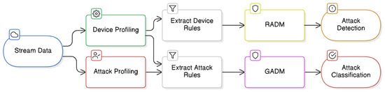
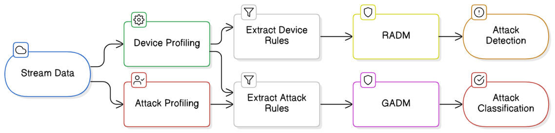
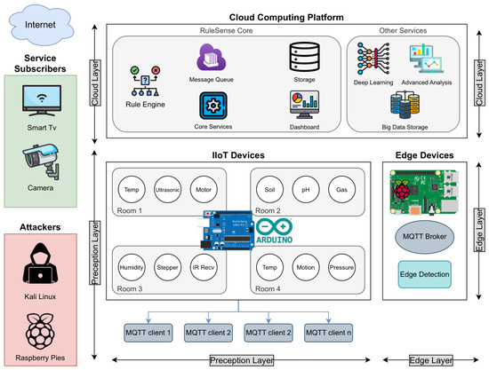
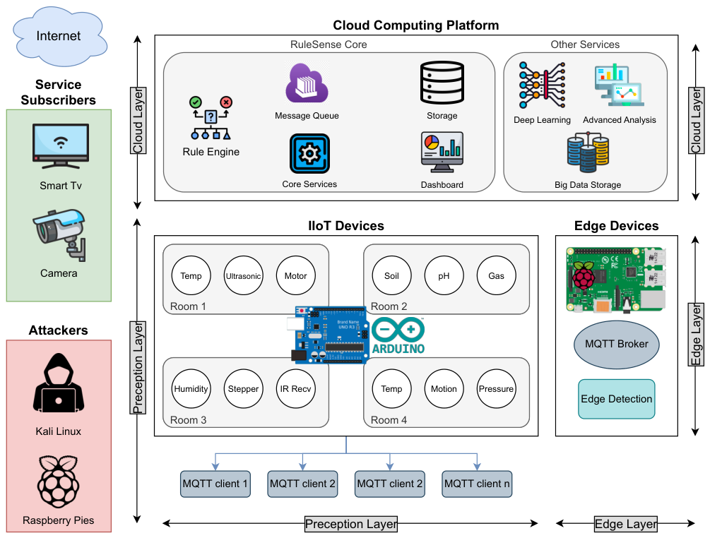
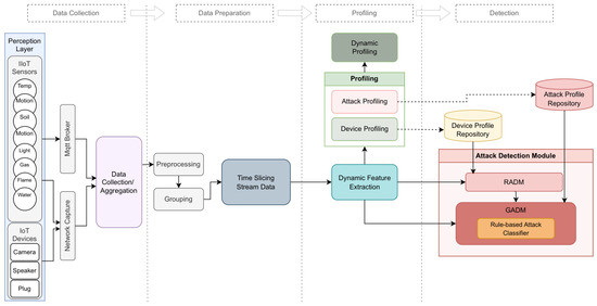
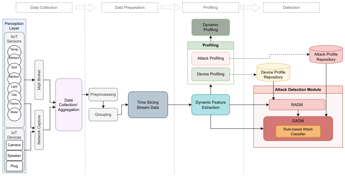
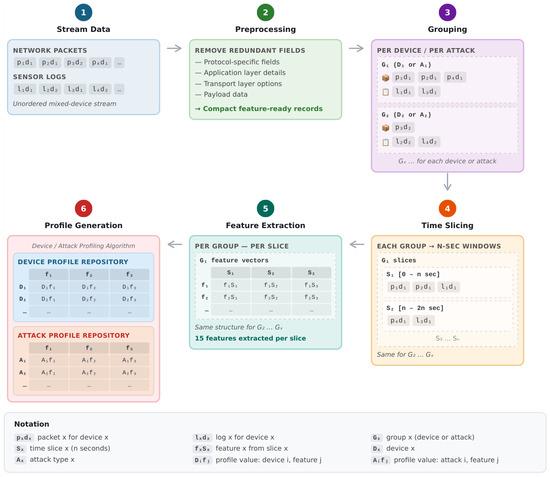
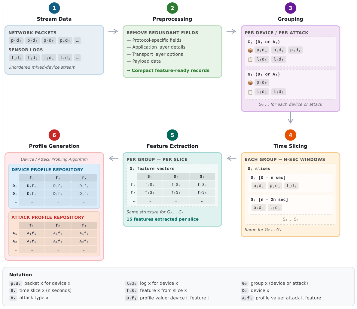
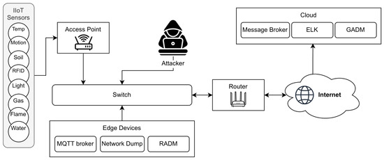
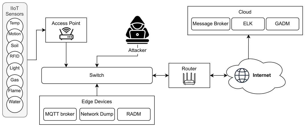
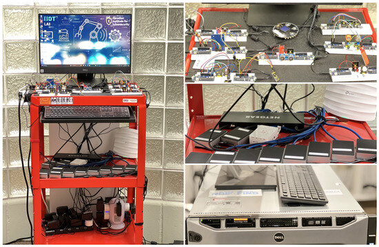
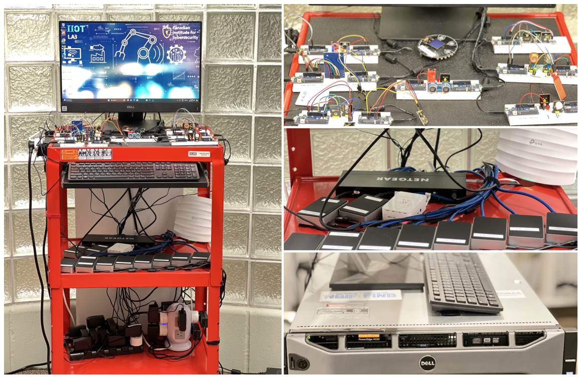
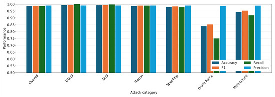
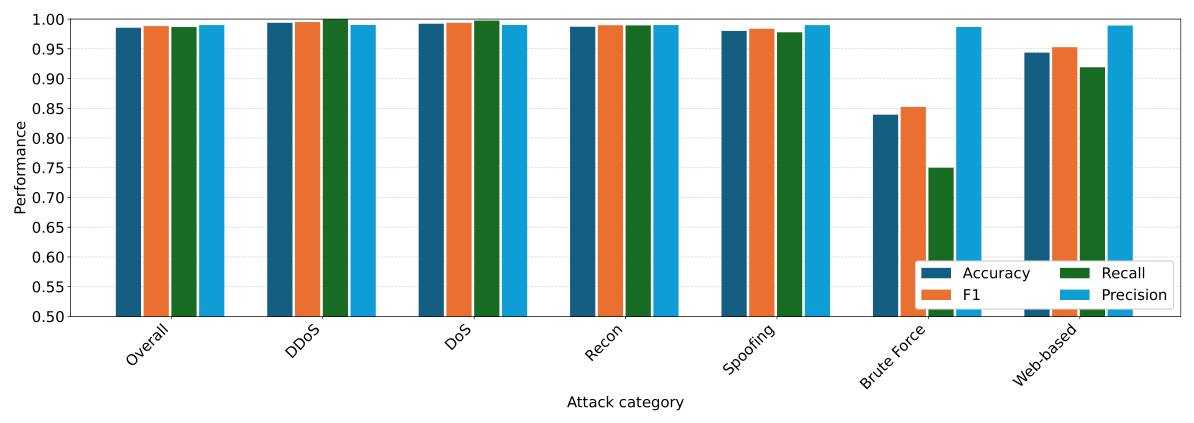
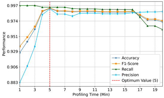
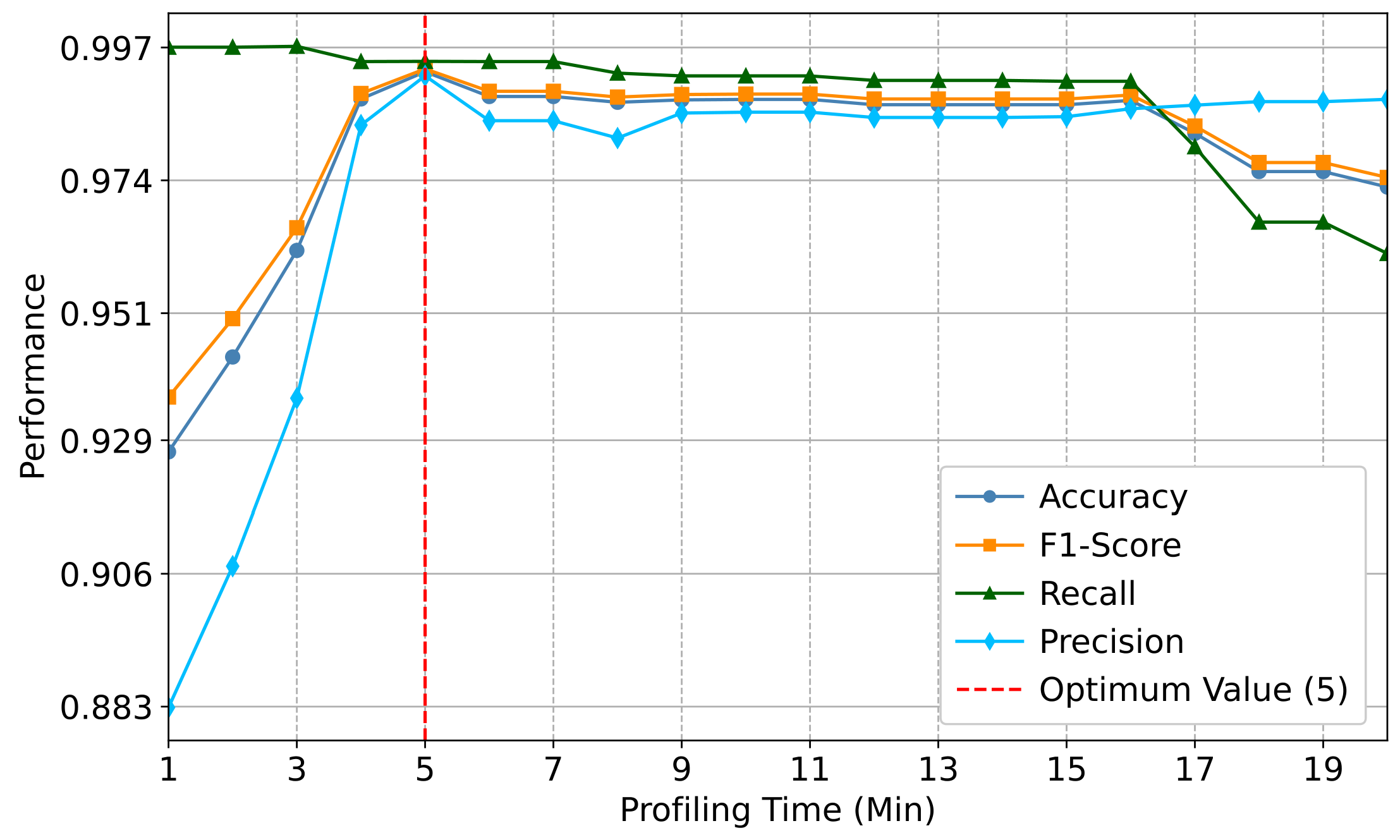
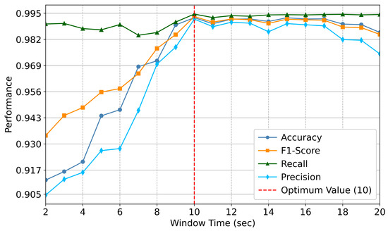
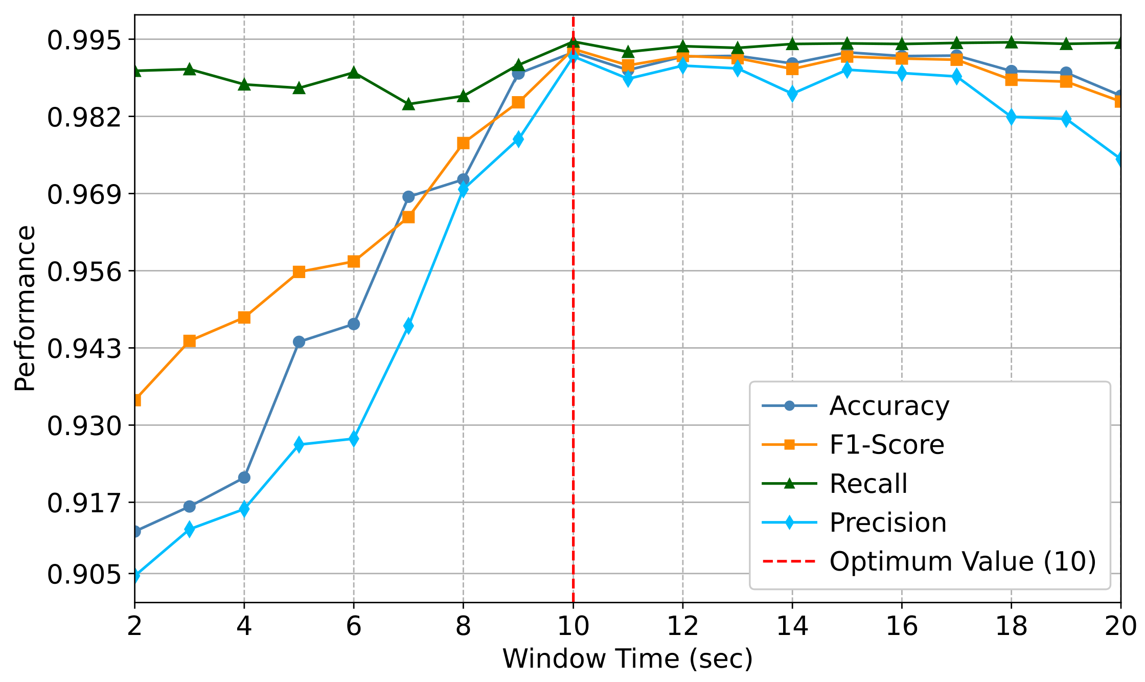
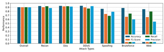
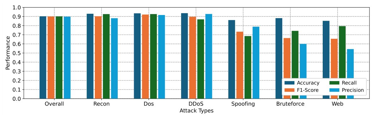
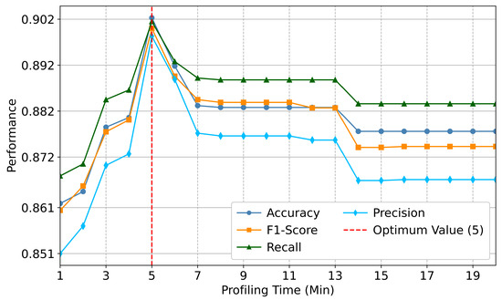
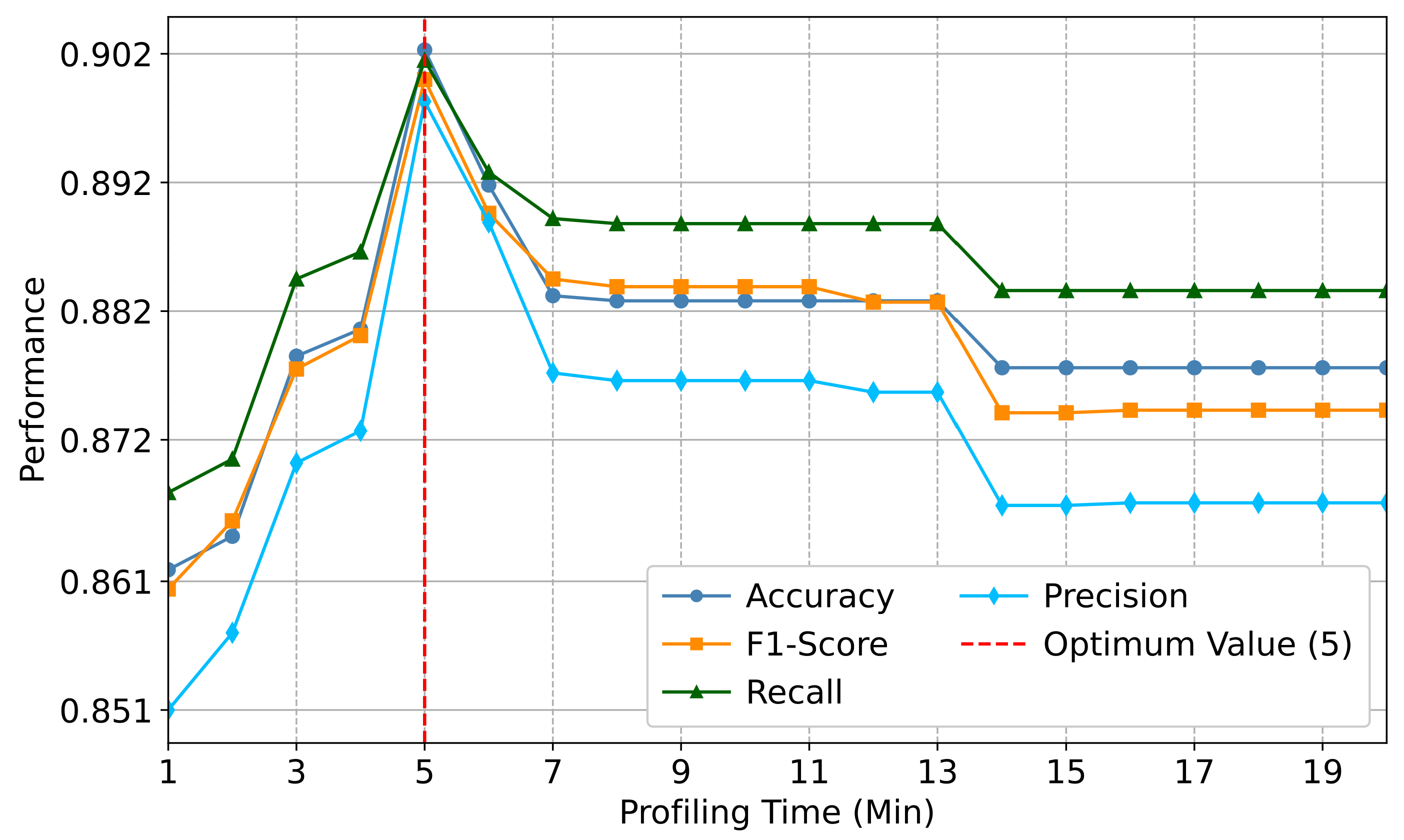
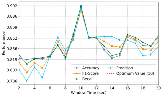
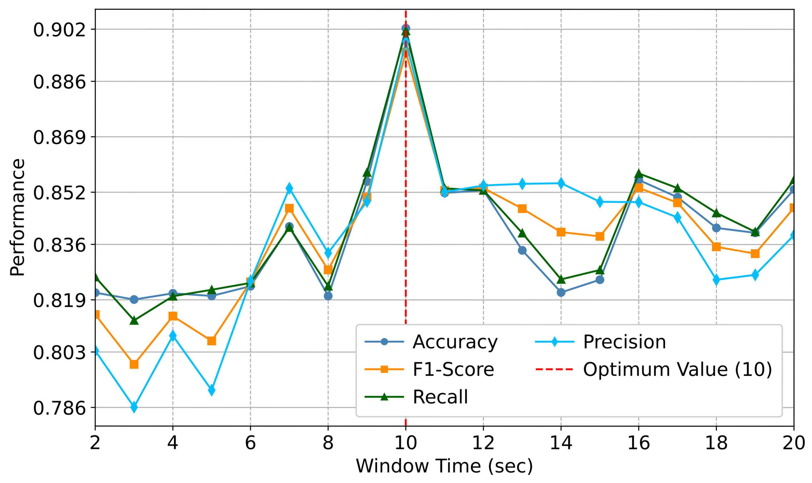
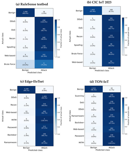
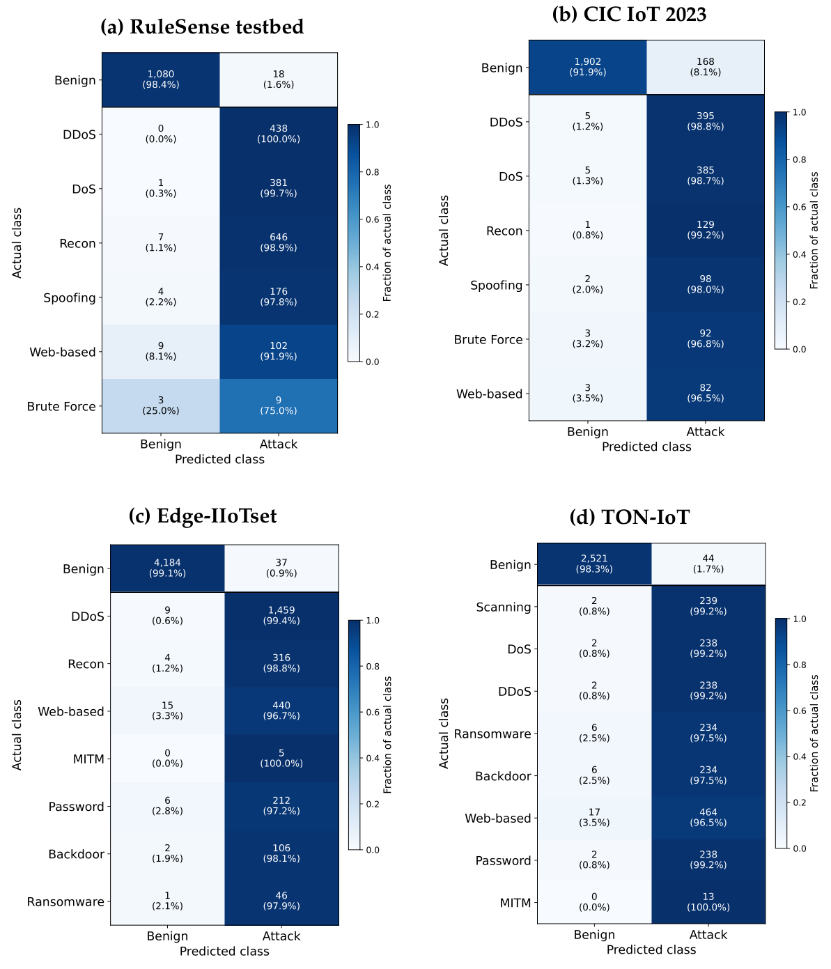
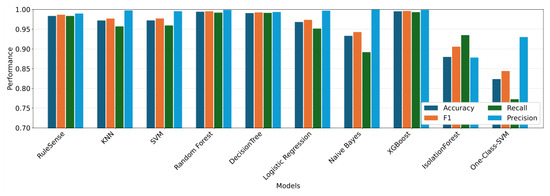
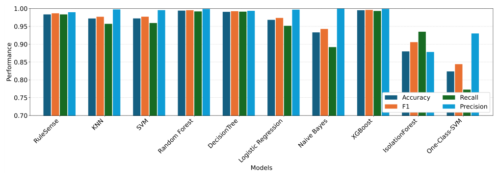
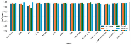
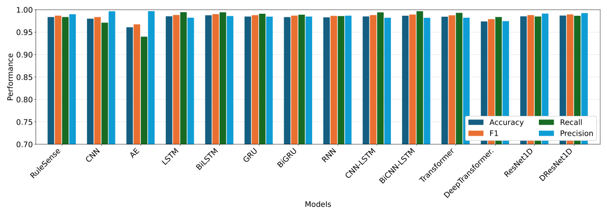
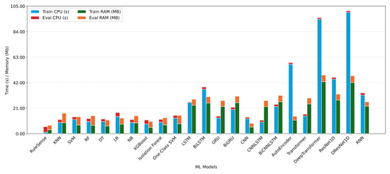
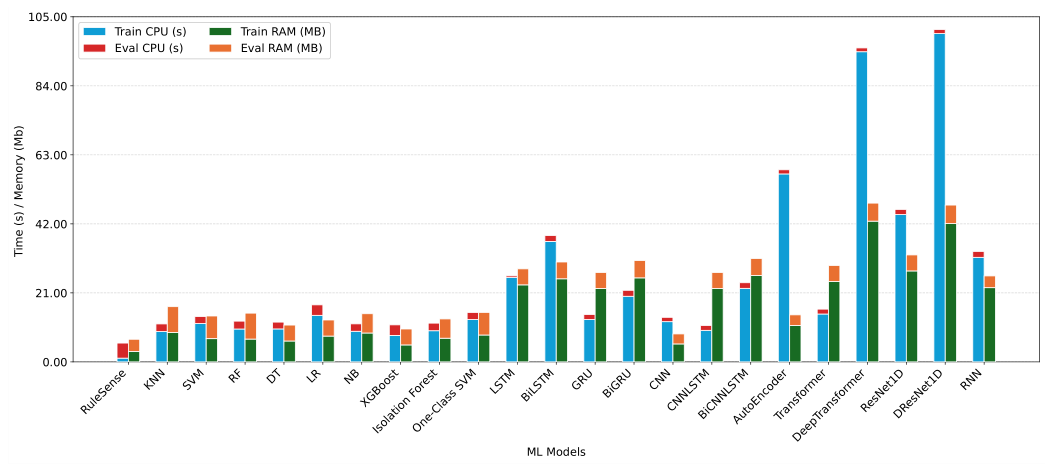
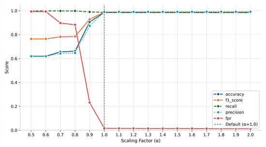
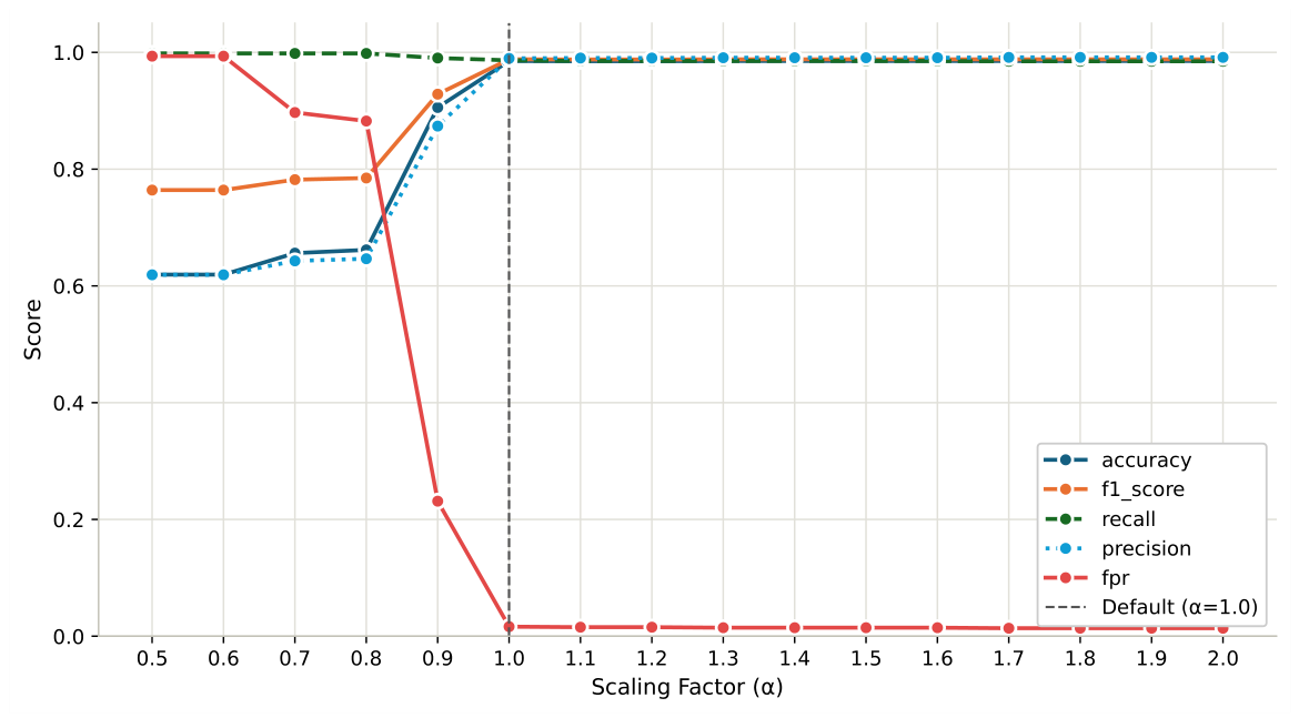

Disclaimer/Publisher’s Note: The statements, opinions and data contained in all publications are solely those of the individual author(s) and contributor(s) and not of MDPI and/or the editor(s). MDPI and/or the editor(s) disclaim responsibility for any injury to people or property resulting from any ideas, methods, instructions or products referred to in the content. |
© 2026 by the authors. Licensee MDPI, Basel, Switzerland. This article is an open access article distributed under the terms and conditions of the Creative Commons Attribution (CC BY) license.