


Abstract
Motor-imagery electroencephalography (EEG) decoding depends on rhythm-specific modulation, cue-locked temporal evolution, and structured electrode topology, yet many decoders treat EEG as a generic multichannel time series. (1) Background: A physiological prior that stays in preprocessing cannot constrain what the decoder represents, and spiking networks let such a prior act on the event code itself. (2) Methods: We introduce PG-SNN, which embeds EEG priors in the event code, spatial operator, temporal dynamics, and readout. A causal eventizer converts EEG into sparse, sign-preserving spikes using rhythm-sensitive, temporal-change, and montage-contrast operators; an electrode-prior graph restricts message passing to local montage adjacency and homologous inter-hemispheric coupling; and a multi-timescale adaptive spiking backbone represents rapid event transitions and slower mu/beta modulation. (3) Results: On BCI Competition IV-2a the model reaches 84.72% accuracy (kappa = 0.796), 2.56 and 5.64 percentage points above the strongest matched ANN and SNN baselines; on the EEGMMIDB four-class subject-independent protocol, it reaches 71.28% (kappa = 0.617), 3.86 points above the strongest matched ANN baseline, and a fifteen-variant ablation attributes the largest single effect to the event code. (4) Conclusions: Embedding sensorimotor physiology into event generation, spatial propagation, and spike dynamics is a practical route to compact motor-imagery decoders, within the limits of the two benchmarks and the single shared protocol.
1. Introduction
Motor-imagery EEG decoding is central to non-invasive brain–computer interfaces (BCIs), neurorehabilitation, and neurophysiological monitoring [1,2]. The discriminative signal is governed by recognizable physiological structure. Imagined movement induces event-related desynchronization and synchronization (ERD/ERS) in the μ and β rhythms [3,4]; that modulation evolves across baseline, cue, and imagery intervals in a cue-locked order, and it is distributed over the sensorimotor strip with contralateral dominance [5]. These properties motivate inductive biases that are difficult to obtain from labels alone. A decoder should preserve the sign of event-related modulation, respond to rhythm-specific changes, restrict spatial exchange according to plausible electrode topology, and represent both transient events and slowly varying rhythm envelopes.
This paper uses physiology-guided in a specific sense: a physiological basis means a neurophysiological mechanism identified by its substrate, its observable scalp signature, and the process it implements, not a general resemblance to cortical anatomy. Three sensorimotor mechanisms are involved, each with a defined substrate, a measurable scalp-level marker, and a corresponding part of the forward map. The first is the modulation of the μ (8–13 Hz) and β (13–30 Hz) rhythms over the sensorimotor cortex that accompanies movement preparation and execution [3,6]. The second is the time course of a motor-imagery trial, where a quiet baseline, a cue, and a sustained imagery interval follow one another while ERD, ERS, and a post-imagery rebound develop in that order [5]. The third is the spatial organization of these effects over the sensorimotor strip, with contralateral dominance near C3 and C4 and a clear left–right symmetry [5].
Deep neural networks have substantially improved EEG decoding by replacing hand-engineered features with trainable spatiotemporal representations. Compact CNNs, shallow and deep convolutional networks, temporal convolutional models, transformer-style decoders, graph-aware networks, and CSP-aware architectures have produced strong performance on motor-imagery benchmarks [7,8,9,10,11,12,13]. Nevertheless, physiological knowledge is often introduced only through preprocessing or post-hoc interpretation. More broadly, trustworthy AI research argues that domain knowledge and physical constraints should be embedded in learning objectives or model architectures, instead of being used only to explain black-box predictions after inference [14]. A model may receive band-pass-filtered signals, yet its event representation and objective may not explicitly encode ERD/ERS directionality or electrode-neighborhood structure. Under limited calibration data, this design leaves the classifier to rediscover known EEG regularities from supervision, which can impair sample efficiency and cross-subject robustness [15,16].
Spiking neural networks (SNNs) provide a natural substrate for event-driven EEG modeling [17]. Membrane states accumulate evidence over time, spikes enable sparse event-selective computation, and adaptive thresholds can regulate persistent activity. Surrogate-gradient learning has made deep SNNs trainable with backpropagation despite the non-differentiability of spike generation [18,19]. Recent residual SNNs [20], hybrid coding methods [21], and spike-driven transformers [22,23] have further improved trainability and temporal expressiveness. SNNs have also been explored for EEG and neural decoding through compact spiking classifiers [24,25,26,27], graph-enhanced SNNs [28], lightweight motor-imagery decoders [29,30], and spiking attention-based decoding [31].
The open question is therefore how EEG physiology should be embedded into spiking computation. A generic SNN can convert samples to spikes and classify the resulting sequence, but it does not specify what constitutes a physiologically meaningful EEG event, which electrodes should exchange information, or how fast and slow components of the signal should be represented. This paper addresses that gap with PG-SNN, a physiology-guided SNN framework for motor-imagery EEG decoding. The aim of this work is to build a decoder whose forward path is organized by the three mechanisms above, and to test under a fixed and fully specified protocol whether those components help decoding relative to matched baselines.
The relevant work falls into four groups. Deep decoders for EEG are the closest line. A second and older tradition encodes physiological structure directly into a decoder. Deployment also depends on the transfer and data-efficiency literature, and spiking networks have their own body of work on biomedical signals. The preceding paragraphs drew on the neurophysiological literature to fix the three mechanisms; the following subsections survey the decoding methods themselves and asks what they already do and where they leave room for the priors. The strands meet where a decoding paper also states a physiological constraint, and those cases are noted as they arise.
1.1. Deep EEG Decoders
Early deep EEG decoders demonstrated that temporal and spatial filters can be learned directly from minimally processed EEG [8,9,32]. Subsequent models expanded this paradigm with multi-branch temporal filters, attention mechanisms, graph operations, and transformer blocks [7,10,11,12,13], and more recent variants combine multiscale temporal attention, attention-based multiscale convolution, and pretrained pipelines that are reused across subjects [33,34,35]. These developments have moved motor-imagery decoding from handcrafted pipelines, such as common spatial patterns, toward end-to-end supervised representation learning [36].
Despite this progress, the physiological structure of motor imagery remains only weakly coupled to many model designs. A temporal convolution may learn frequency-selective filters without maintaining a stable relationship to the μ and β bands. A spatial convolution may mix channels without respecting electrode geometry. Transfer learning, augmentation, and pretraining studies further show that data efficiency and inter-subject variability remain persistent limitations [16,37]. These observations motivate explicit prior injection instead of relying entirely on label-driven discovery.
1.2. Physiological Priors and Structure in EEG Decoding
A second and older line of work encodes physiological or anatomical structure directly into the decoder instead of leaving it to be discovered from labels. Common spatial patterns and their filter-bank variants derive spatial filters under an explicit variance-ratio criterion [38,39]; Laplacian montage filters impose a fixed local spatial operator; Riemannian methods classify the spatial covariance itself rather than a feature vector derived from it [40]; and graph-based models extend the same idea to message passing over an electrode adjacency [11,12,28]. In all of these, the physiological content enters as structure: a fixed operator, a fixed criterion, or a constrained connectivity. Training cannot trade it away.
The priors used here belong to that lineage, and Section 2 states for each of them whether it is enforced as structure or as a penalty. Two choices distinguish this design from the spatial-filter tradition. First, the prior acts on the event code rather than only on the input: which samples become events is decided by the rhythm bands, by the sign of the modulation, and by the montage contrast, so the physiological content is carried into the spiking representation instead of being confined to a preprocessing stage. Second, the graph prior is used twice, once as a forward operator and once as a regularizer on the latent state, so it shapes the representation and not only the input. The neurophysiological substrate that these choices are meant to reflect is documented in the ERD/ERS literature [3,4,5], including the motor-planning component [41].
1.3. Cross-Subject Transfer and Data Efficiency
In practice a motor-imagery decoder is limited less by its peak accuracy than by the calibration it demands, and a large volume of literature addresses that constraint. Transfer learning and domain adaptation reduce the number of target-subject trials by aligning distributions across sessions or subjects, either in feature space or in the space of spatial covariances [40,42]; federated schemes go further and train across subjects without pooling the raw signals [43]. Data augmentation and knowledge-driven channel manipulation help when target data are scarce [16,34], and pretrained models amortize the cost of fitting a decoder for a new subject [35].
These methods complement prior injection; they do not replace it. Alignment removes distribution shift but does not change what the decoder represents, and a decoder whose forward path already encodes the physiological structure of the task should need less calibration data to reach a given accuracy, which is the effect Section 3.4 tests under reduced labels and leave-one-subject-out evaluation [37].
1.4. SNN Training and Biomedical SNNs
SNN research has advanced from shallow spiking classifiers and ANN-to-SNN conversion toward directly trained deep SNNs, a transition surveyed in [44]. Surrogate-gradient learning is the dominant supervised training strategy because it approximates the derivative of the Heaviside spike function while retaining binary spikes in the forward pass [18,19]. Recent architectures use residual connections, hybrid coding [21], adaptive thresholding [45], spike-driven attention [22,23,46], and lightweight or low-latency training schemes [47,48], and consolidated training recipes have made direct training routine [49]. At the same time, comparative studies emphasize that SNN efficiency depends on the coding scheme, the number of time steps, active operations, and the hardware model used for measurement [50], which is why the efficiency figures reported here are operation counts, not energy.
In EEG and biomedical signal recognition, SNNs have shown promise for sparse temporal decoding, compact inference, graph-based propagation, multimodal physiological fusion, and information-bottleneck-driven representation learning [24,25,26,27,28,51]. Reported applications span motor imagery [29,30], auditory attention decoding [31], intracortical signal decoding [52], and emotion recognition from physiological signals [53]. However, many EEG-SNN designs remain architecture-centric: they modify coding schemes or spiking layers without explicitly linking event generation to EEG rhythm physiology and electrode topology. PG-SNN is positioned at this intersection. It retains spiking computation, but its central design objective is to encode EEG-specific priors directly into the forward path, as surveyed in the systematic reviews of this area [54].
2. Materials and Methods
2.1. Problem Formulation and Overall Architecture
Let an EEG trial be denoted by X ∈ ℝC×T, where C is the number of electrodes and T is the number of time samples. The corresponding label is y ∈ {1,…,K}, where K is the number of classes. The model outputs a categorical probability vector ŷ = fΘ(X), where Θ collects all trainable parameters.
The model has four parts. An EEG-aware eventizer converts the trial into sparse, sign-preserving events. An electrode-prior graph encodes spatial structure over the montage. A topology-aware multi-timescale spiking backbone carries those events through time. A task-interval readout, trained with a composite objective, produces the class probabilities. Figure 1 shows the overall architecture, and each part is detailed below. A physiological prior can enter the model in one of two ways, and we keep the two apart. Part of the structure is built into the forward map: events are computed only from causal band-limited operators, spatial mixing goes through the electrode graph, and the readout summarizes by scalp region. This restricts what the model can represent without pinning any value, since the filter coefficients, thresholds, graph weights, and attention weights all stay trainable. The sign-preserving dual-polarity events and the montage k-NN adjacency with homologous links are of this form; the rhythm filters start as fixed band-pass operators but remain trainable, so their band-limited character is encouraged by the out-of-band penalty rather than guaranteed by structure. The rest of the priors enter the training objective as penalty terms—topology smoothing, spike sparsity, and the out-of-band filter penalty—each weighted by a coefficient selected on the validation set, and any of those coefficients can be driven to zero by that selection. Table 1 records which of the two applies to each of the three mechanisms, and Section 3.4 reports what removing each one costs.
Figure 1.
Overview of the proposed physiology-guided SNN for EEG decoding. Continuous EEG is converted into sparse-rhythm, temporal-change, and montage-contrast events, which are processed by an EEG-prior graph and a topology-aware spiking backbone, then classified by a task-interval readout. The event tensor produced by the eventizer is denoted Z0[t], and the readout panel shows the temporal attention over the task interval defined in Section 2.4.
Table 1.
The three sensorimotor mechanisms of Section 1, the observable that carries each one, the part of the forward map that encodes it, how the prior is enforced, and the ablation that tests it.
2.2. EEG Prior Encoding: Eventization and Electrode Graph
Instead of converting EEG into spikes through generic rate coding, the proposed eventizer first applies an EEG-aware operator bank to the input trial. The bank combines rhythm-sensitive, temporal-change, and montage-contrast operators, and the resulting drives are converted into sparse, sign-preserving events. The electrode graph then supplies the spatial structure used by the spiking backbone.
2.2.1. Causality-Aware and Sign-Preserving Eventization
The eventizer is causal: the output at time t depends only on the input up to t, so the event code can be produced in a streaming fashion. This property applies to the eventizer alone; the readout of Section 2.4 aggregates over the whole task interval and is therefore not by itself an online decoder. Events are generated by threshold crossings relative to a running reference, and both polarities are kept: a deflection above its reference produces a positive event and a deflection below it produces a negative event.
oc,j[t] = φj(X1:t)c,
Because the operator bank mixes descriptors of different scale, each operator is normalized before thresholding.
The statistics μ and σ are estimated per channel and per operator on the training set and reused unchanged at validation and test time; in cross-subject protocols they are computed only from the available training subjects.
Here 0 < λ < 1. The one-step update keeps the current sample from serving as its own reference.
Here θj > 0 is the event threshold and γj > 0 controls the trigger sharpness; both are parameterized as positive quantities and initialized from training-set quantiles of |õ − |. During training the derivative of the Heaviside function is replaced by a surrogate gradient.
Keeping the sign preserves the polarity of the band-limited signal around its running reference, instead of collapsing it through a magnitude transform. We do not equate this polarity with the ERD/ERS index itself: ERD/ERS is defined as a change in band power relative to a baseline, whereas the eventizer operates on the signed band-limited waveform and its running reference. The two are related in that both track the same rhythm-band modulation, but the event code is a signed-threshold surrogate for that modulation rather than a direct estimate of the ERD/ERS ratio. The threshold is calibrated on the training set, and the event grid is subsampled by a stride—5 samples in the reported configuration, i.e., 20 ms for the 250 Hz BCI IV-2a signals and 31.25 ms for the 160 Hz EEGMMIDB signals—which trades temporal resolution against training cost; the selected value fixes the discretization of every reported run. Collecting the signed event codes over channels and time gives the event tensor Z0[t], which is the input to the first spiking layer.
2.2.2. Rhythm, Temporal-Change, and Montage-Contrast Operators
The operator bank encodes three complementary EEG cues. The first cue is rhythm-sensitive activity: for each rhythm band, a causal FIR temporal filter is initialized as a windowed band-pass filter and is regularized to remain within the task-relevant passband; the default banks are 8–13 Hz for μ and 13–30 Hz for β. The second cue is temporal change: a short-window difference operator responds to transitions in the signal, aligning the event code with the cue-locked time course of a trial. The third cue is montage contrast: a topology-aware Laplacian operator compares each electrode with its immediate neighborhood, so that local spatial departures, not absolute amplitude, drive event generation.
The three drives are combined and converted into sparse events, so that what enters the spiking backbone is a physiologically structured event code rather than a generic rate representation.
Here ωb[τ] is a causal smoothing window and ε > 0 prevents numerical instability.
dc,b[t] = pc,b[t] − pc,b[t − Δb]
Here Lg is the normalized graph Laplacian and pb the band-power vector.
𝓁b[t] = Lgpb[t]
ΦEEG = {xb,pb,db,|db|,𝓁b:b ∈ EEG}
No sample after time t enters Equation (8), so the filter stays causal. The out-of-band penalty is
2.2.3. Electrode-Prior Graph
The EEG prior graph GEEG = (V, E, A) has one node per electrode. When three-dimensional electrode coordinates are available, distances between normalized scalp coordinates define geometric proximity; when only a standard montage name is available, the corresponding 10–20 or 10–10 template coordinates projected onto a unit sphere are used. The adjacency combines geometric proximity with homologous inter-hemispheric pairing (k-nearest-neighbor adjacency with k = 4).
Here Nk(i) is the k-nearest-neighbor set of electrode i, π(i) its approximate homolog in the opposite hemisphere, and ηsym ≥ 0 the pairing strength; midline electrodes carry no homologous term.
A weighted variant reduces smoothing across homologous pairs so that the representation can be locally smooth while preserving left–right asymmetry.
Equation (11) uses the symmetrized adjacency without self-loops, whereas Equation (15) adds self-loops and normalizes for spiking propagation.
The hyperparameters introduced by the physiological constraints are few and each has a bounded search space that is fixed before test evaluation. Table 2 lists them. The neighborhood size k and the kernel width σd of the electrode graph are the only free structural parameters; membrane thresholds and trace time constants are model parameters learned during training rather than selected per subject, and the number of traces Q and the diffusion order P are discrete architectural choices evaluated in the ablation of Section 3.4. Every value is selected once on the validation partition and then held fixed, so the cost of the selection is a one-off model-design step and not a per-subject calibration procedure.
Table 2.
Search space of the graph-construction hyperparameters. The value used in the reported configuration is selected on the validation partition; the search space itself is fixed before any test evaluation, and the same space is applied to every subject.
2.3. Topology-Aware Multi-Timescale Spiking Backbone
At each spiking layer, the input current is computed by graph-based diffusion of the previous layer’s spike state: a trainable weight matrix is applied per diffusion order, and the orders are combined so that information propagates over the electrode adjacency rather than through all-to-all channel mixing. The default diffusion order is P = 2; setting P = 0 removes graph propagation entirely.
Here Zℓ−1 is the previous layer’s spike state, Wp the weights for diffusion order p, and b a bias term.
EEG contains rapid event changes and slower rhythm-level modulation. To capture this heterogeneity, each spiking layer uses a finite bank of exponential traces (Q = 4 by default), each with its own learnable time constant; the traces are mixed by learned gates to form the effective membrane drive, and neurons emit spikes when the membrane potential exceeds an adaptive threshold. The bank lets fast event dynamics and the slower μ and β envelopes be represented in one pass rather than in separate branches. The backbone is trained end-to-end by backpropagation through time with a fast-sigmoid surrogate gradient.
Here 0 < ρ < 1 determines the trace time constant.
Here Δt is the time step. The coefficient α in Equation (20) is parameterized on the same physical time scale as the trace and threshold decays, so a change in Δt changes the numerical resolution rather than the membrane time constant. The time constants are spread on a logarithmic grid so that the bank covers both fast event transitions and slower rhythm modulation, and they are clipped to a fixed range that keeps every trace away from the sampling step at one end and from a constant at the other.
The trace mixture uses nonnegative normalized coefficients
Here 0 < α < 1, ⊙ denotes element-wise multiplication, and Θ is the adaptive threshold. The delayed reset in Equation (20) avoids an implicit algebraic loop between the current membrane potential, spike and reset, while still suppressing sustained firing at the next step.
The current spike is generated from the previous threshold:
Z𝓁[t] = (U𝓁[t] − Θ𝓁[t − 1])
The threshold trace is then updated by
and the adaptive threshold is
Here 0 < κ < 1, and β is nonnegative and bounded above. The adaptive threshold suppresses persistent over-firing and supports sparse event-selective computation; the trace bank separates the synaptic filtering time scale from the membrane-leak time scale, so fast onsets and slow envelopes are represented without additional recurrent layers.
Since the spike states are binary, the input current obeys the following bound, which is finite whenever the graph weights and biases are bounded:
The bound is finite under the stated assumptions: Equation (17) is an exponentially stable recursion driven by a bounded input, the mixture coefficients are nonnegative and sum to one, and Equations (20)–(23) are stable with bounded inputs, so the bound follows by induction over layers.
2.4. Readout and Training Objective
Let ZL[t] be the output spikes of the last spiking layer. A causal smoothing of the spike stream forms a latent state; instead of uniform temporal averaging, the readout learns a temporal attention over the task interval, supplemented by region-aware spatial attention over sensorimotor, midline, frontal, and parietal electrode groupings, and by a rhythm-guided log-bandpower pathway. The pooled representation is classified by a linear layer producing class probabilities.
R[t] = λrR[t − 1] + (1 − λr)ZL[t]
Here 0 < λr < 1.
Here t ∈ Ttask, and Poolc denotes global channel pooling used only to compute the attention score.
For the region-aware readout, let {} denote the predefined scalp regions:
The regional feature is
If reliable region definitions are unavailable for a montage, Equation (28) is replaced by global average pooling over electrodes.
Here p is the causal log-bandpower descriptor of Equation (9) before thresholding.
The training objective combines the cross-entropy loss with three regularizers. The topology regularizer encourages local smoothness of latent states over physiologically adjacent electrodes, while a weighted smoothing matrix reduces smoothing across homologous pairs so that discriminative hemispheric asymmetry is not erased. The spike-sparsity penalty controls layer activity, tying the computational cost of the backbone to its binary state rather than only to its weights. An out-of-band filter penalty keeps the causal rhythm filters within their intended passbands.
Here 0 ≤ ξsym ≤ 1 reduces smoothing across homologous pairs to avoid excessive inter-hemispheric smoothing.
= cls + λtopotopo + λspkspk + λfiltfilt
Training uses backpropagation through time with surrogate gradients for event and neuron spikes; inference uses the same forward path as Equation (1).
The default weights are λtopo = 0.01, λspk = 5×10⁻⁴, and λfilt = 1×10⁻⁴, selected on the validation partition from coarse grids.
3. Results
This section reports the experimental study of the pipeline specified in Section 2. The pipeline is instantiated with the model assumptions of Section 2 and with the acquisition and evaluation settings of the two benchmarks. The paired comparisons require the evaluation pipeline to be held fixed, with the same splits, seeds, channel normalization, and model-selection rule applied to every method. This isolates the effect of the modeled priors from differences in evaluation settings.
3.1. Datasets and Preprocessing
Two public motor-imagery EEG benchmarks are used in the evaluation, i.e., BCI Competition IV-2a [55] and EEGMMIDB [56]. Both datasets are publicly available and de-identified, and both were collected in earlier studies under their own ethics approvals; no new signals were recorded for the present work. BCI Competition IV-2a contains nine right-handed subjects without known neurological disorders (one female and eight males, aged 22–35), 22 EEG channels, four motor-imagery classes, and separate training and evaluation sessions containing 288 trials each. For the subject-dependent protocol, the training session is split into training and validation partitions with stratified labels, and the official evaluation session is used only once for testing. For the cross-subject protocol, leave-one-subject-out training is used, and all normalization statistics are estimated only from the training subjects.
EEGMMIDB is evaluated at 160 Hz under protocol-specific motor-imagery settings on the 109 healthy volunteers of the PhysioNet release: left-versus-right fist imagery, both-fists-versus-both-feet imagery, and four-class imagery. Both subject-independent and subject-specific fine-tuning settings are reported because performance changes substantially with the number of classes and with access to subject-specific calibration trials. Subject characteristics are summarized in Table 3; the EEGMMIDB public release does not distribute per-subject demographic fields.
Table 3.
Characteristics of the two benchmark datasets. Values are those documented with the public releases; the EEGMMIDB release does not distribute per-subject demographic fields (n.r. = not released).
The two benchmarks follow different cue-locked motor-imagery paradigms, and their trial timelines are summarized in Figure 2. In BCI IV-2a, each trial opens with a fixation cross (0–2 s); a directional cue then appears at 2 s and remains visible for 1.25 s, while the subject performs the indicated motor imagery until the trial reaches 6 s; and the trial closes with a short break before the next trial. In EEGMMIDB, each run alternates between a resting baseline (annotated T0) and a 4 s task interval (annotated T1/T2, whose meaning depends on the run: in the left/right-fist runs T1 and T2 denote left-fist and right-fist imagery, whereas in the both-fists/both-feet runs they denote both-fists and both-feet imagery), and each epoch is anchored at the task onset. In both datasets the discriminative interval is cue-locked and of fixed length, so a fixed-window comparison between methods is meaningful.
Figure 2.
Trial timelines of the two benchmarks. (a) In BCI Competition IV-2a a fixation cross is followed by a directional cue at 2 s and a 4 s imagery interval, then a break. (b) In EEGMMIDB each run alternates between a resting baseline (T0) and a task interval (T1/T2).
All trials are cropped relative to the official motor-imagery annotations. For BCI IV-2a, a 5.0 s window beginning 1.0 s before the cue is used, and the task readout interval excludes the pre-cue baseline. For EEGMMIDB, a 4.0 s window beginning at the annotated imagery event is used. The input is re-referenced using the dataset-provided montage and then normalized with channel-wise statistics estimated from the corresponding training split. No validation-trial or test-trial statistics are used to fit the normalization parameters, preventing leakage and keeping the preprocessing consistent with the causal eventization of Section 2.2.
3.2. Implementation Details, Baselines, and Evaluation Metrics
The default PG-SNN uses two topology-aware spiking layers, hidden width 32, graph diffusion order P = 2, Q = 4 exponential traces, temporal attention, region-aware spatial attention, and the rhythm-guided log-bandpower readout. The selected rhythm bands are 8–13 Hz for μ and 13–30 Hz for β, with the 13 Hz boundary shared by the two bands. The model is trained with AdamW (batch size 32), cosine learning-rate decay, early stopping on validation macro-F1, gradient clipping, and surrogate-gradient backpropagation through time. The regularization weights are selected on the validation set from coarse grids (λtopo ∈ {0, 10−4, 10−3, 10−2}, λspk ∈ {0, 10−4, 5 × 10⁻⁴, 10−3}, λfilt ∈ {0, 10−4, 10−3}); the reported configuration came out of a small but systematic search rather than a single hand-tuned setting. The search varied the graph diffusion order (P ∈ {0,1,2,3}), the number of traces (Q ∈ {1,2,4}), the hidden width (d ∈ {16,32,64}), the learning rate ({5 × 10⁻⁴, 1 × 10⁻³, 2 × 10⁻³}), and the event-grid time step. Every hyperparameter, including those of the baselines, was chosen on the validation partition. Each setting is repeated with five random seeds, and the same seeds are used for all matched baselines. On the validation partition the selected configuration (d = 32, P = 2, Q = 4, learning rate 1 × 10⁻³) ranked first within every one-dimensional slice of the grid, and the nearest alternatives (d = 64, P = 1, Q = 2, and a learning rate of 2 × 10⁻³) each lost between 0.3 and 1.1 points of validation macro-F1 relative to the selected setting. The grid is coarse on purpose: the aim is one shared protocol for every method rather than the best score for any single one of them.
The matched baselines include CSP+LDA [38,57], FBCSP+SVM [39,58], EEGNet [9], ShallowConvNet and DeepConvNet [8], TCNet [59], CTNet [60], a directly trained LIF-SNN [18,19], and a Graph-LIF SNN [28]. All neural baselines use the same train/validation/test splits, the same channel normalization policy, and the same model-selection rule. The primary metrics are accuracy, Cohen’s κ, macro-f1, and balanced accuracy. Balanced accuracy is the mean of the per-class recall values, so on a class-balanced evaluation set it is identical to accuracy by construction; the two columns are reported side by side for completeness. Accuracy, balanced accuracy, and macro-f1 are all derived from the same confusion matrix and are therefore not independent evidence. Efficiency is reported by trainable parameters, dense multiply–accumulate operations (MACs) for ANN baselines, synaptic operations (SynOps) for SNN baselines, and event/spike rate under the same input length and batch size. Statistical comparisons are performed on subject-level paired results with a two-sided Wilcoxon signed-rank test and Holm–Bonferroni correction; trial-level samples are not used as independent observations.
3.3. Main Results and Statistical Comparisons
The subject-wise PG-SNN results under the BCI IV-2a subject-dependent protocol are reported in Table 4. The full-model mean is 84.72% accuracy (95% confidence interval 80.50–88.94 over the nine subjects) and κ = 0.796, with per-subject accuracy ranging from 76.39% to 91.67%. Reporting every subject is necessary because BCI IV-2a contains substantial inter-subject variability and the group-level comparison is what the statistical tests operate on.
Table 4.
Subject-wise BCI IV-2a PG-SNN results under the official subject-dependent protocol.
PG-SNN is compared with the matched baselines in Table 5. The proposed model exceeds the strongest ANN baseline by 2.56 percentage points in accuracy and the strongest reproduced SNN baseline by 5.64 percentage points. The gain over the Graph-LIF SNN shows that graph propagation alone does not account for the full difference under this fixed protocol. Because that comparison also changes model capacity, readout, and regularization, it establishes that the other components contribute as a group. The contribution of each one separately is isolated in the ablation of Section 3.4.
Table 5.
Matched baseline comparison on BCI IV-2a. Values are subject-level means ± standard deviation over nine subjects and five random seeds.
Protocol-specific EEGMMIDB results are reported in Table 6. The two-class settings are easier than the four-class setting, and subject-specific fine-tuning further improves PG-SNN in both settings. The fine-tuning block is reported for PG-SNN only, because the baselines were evaluated under the subject-independent protocol; the cross-method comparison is therefore the subject-independent block above, and the fine-tuning rows document the effect of calibration for PG-SNN rather than a matched baseline comparison. Under the subject-independent four-class protocol, PG-SNN reaches 71.28% accuracy, which is 5.10 percentage points above the Graph-LIF SNN baseline. This protocol-specific reporting avoids mixing class definitions and validation settings into a single aggregate score.
Table 6.
Protocol-specific EEGMMIDB matched results. CTNet is reported for the BCI IV-2a protocol only, because its convolutional tokenizer is defined for a fixed input geometry (22 electrodes, 250 Hz) and no configuration of that tokenizer is defined in the original description for a 64-channel montage; re-implementing it for EEGMMIDB would have changed it into a different model and broken the like-for-like baseline comparison. The cross-method comparison in this table is therefore the subject-independent block, in which all other baselines were run under one shared protocol.
Statistical comparisons. The paired statistical comparisons against the strongest reproduced baselines are reported in Table 7. For BCI IV-2a, the paired unit is the subject-level mean across seeds. For EEGMMIDB, the paired unit is the held-out subject in the leave-subject-out protocol. After Holm–Bonferroni correction, the differences remain significant against the strongest matched ANN baseline and the strongest matched SNN baseline in the primary BCI IV-2a and EEGMMIDB four-class settings. These tests are performed on subject-level pairs and treat the subject as the unit of evidence.
Table 7.
Paired statistical tests for the primary comparisons (two-sided Wilcoxon signed-rank tests on paired subject-level results; the adjusted p-values are Holm–Bonferroni-corrected across the six primary comparisons reported here, which constitute the correction family; the remaining baseline comparisons in Table 5 and Table 6 are descriptive and are not included in that family). The paired unit is the subject, so each BCI IV-2a comparison rests on nine pairs and the smallest attainable two-sided p-value is 2/29 ≈ 0.0039; the BCI IV-2a p-values are reported at that granularity.
3.4. Ablation and Generalization Analysis
3.4.1. Component Ablation
Each prior is removed or replaced in turn while the rest of the pipeline is held fixed: the same splits, the same channel normalization, the same model-selection rule, and the same five random seeds as the full model. Fifteen configurations are compared under the BCI Competition IV-2a subject-dependent protocol, and Table 8 reports mean accuracy, the difference from the full model, and the mean layer spike rate for each. This is the test that Table 1 implies: if an explicitly encoded physiological prior helps, removing it should cost accuracy; if it does not, the cost should be zero.
Table 8.
Component ablation on BCI IV-2a under the subject-dependent protocol. Each row removes or replaces one component and keeps the rest of the pipeline fixed. Δ is the difference in mean accuracy from the full model; spike rate is the mean layer spike rate over the same runs. Values are mean ± standard deviation over nine subjects and five seeds.
The event code carries the largest effect. Replacing the EEG-specific eventizer with generic rate coding lowers accuracy from 84.72% to 80.43%, a drop of 4.29 points, and raises the layer spike rate from 0.094 to 0.172. A rate code emits events continuously rather than at threshold crossings of a band-limited operator, so it loses accuracy and costs more computation at the same time. Discarding the sign while keeping the magnitude costs 2.41 points, which places part of the effect in the sign-preserving form rather than in thresholding alone.
Within the operator bank, removing the β branch costs 2.74 points, and removing the temporal-change or montage-contrast operators costs 1.86 and 1.68. The spatial-contrast operator contributes independently of the graph that follows it, which is why the two are ablated separately.
On the graph side, removing propagation costs 1.96 points; reducing the diffusion to first order costs 0.81 and raising it to third order 0.66, so the default P = 2 is the best of the three settings tested. Removing the homologous links costs 1.03 points, consistent with the lateralization reported in Section 3.5.
Collapsing the multi-timescale bank to a single LIF trace costs 2.44 points, the third largest effect in the table, and removing the adaptive threshold costs 1.57 while raising the spike rate to 0.156. The two regularizers act on different quantities: removing the topology term costs 1.24 points, whereas removing the spike-sparsity penalty costs only 0.53 points but multiplies the layer spike rate by 3.6, from 0.094 to 0.339, which is what that term was introduced to control. Replacing the rhythm-guided readout with the plain attention readout costs 1.45 points.
Taken together, the ablations order the components in the sequence the design implies: the event code first, the temporal bank and the rhythm prior next, the graph third, and the regularizers last. Each of the three mechanisms of Section 1 therefore has a component whose removal is measurable.
3.4.2. Generalization Under Reduced Labels and Cross-Subject Transfer
Robustness under reduced labels and cross-subject transfer is reported in Table 9. The margin over the strongest baseline is clearly larger in the 25% label setting than in the full-data setting and is comparable at 50%, which is consistent with the intended role of physiology-guided priors as sample-efficiency constraints. The leave-one-subject-out setting remains substantially harder than subject-dependent evaluation, but PG-SNN preserves a consistent advantage over matched ANN and SNN baselines.
Table 9.
Low-data and cross-subject generalization results. The baselines listed here are a representative subset of those in Table 5; CTNet was evaluated on the BCI IV-2a protocols only and is therefore not reported for the EEGMMIDB column.
3.5. Efficiency, Event Sparsity, and Physiological Interpretability
Efficiency under the same input length, batch size, and timing protocol is reported in Table 10. Latency is deliberately not reported and is not treated as an energy proxy, because GPU and CPU latency include framework overhead and do not represent neuromorphic hardware execution. The main efficiency indicators for SNNs are event rate, layer spike rate, and SynOps. PG-SNN uses more parameters than EEGNet, but under the same input length and batch size its active operation count is well below that of the dense convolutional baselines, because sparse events suppress most layer updates.
Table 10.
Efficiency and sparsity comparison under matched input length.
Physiology-alignment metrics computed over test trials are summarized in Table 11. Sensorimotor ROI concentration measures the fraction of readout saliency assigned to C3/Cz/C4 and neighboring electrodes. The lateralization index compares contralateral and ipsilateral sensorimotor activity for left- and right-hand imagery. The full PG-SNN produces higher ROI concentration and a stronger contralateral lateralization index than the rhythm- or graph-ablated models. These analyses support the claim that the priors affect the internal representation, while avoiding any claim of source-level neural reconstruction. This is a check on the model’s internal representation, not an independent physiological validation: the same graph and region-aware readout that the model is trained with are the ones whose effects these metrics summarize.
Table 11.
Physiology-alignment analysis on BCI IV-2a. ROI concentration is computed over sensorimotor electrodes and their first-order neighbors; topology smoothness is a normalized inverse graph–Laplacian energy.
Qualitative evidence for the internal mechanisms behind the quantitative results in Table 11 and Table 12 is provided in Figure 3, Figure 4, Figure 5 and Figure 6. They are used to inspect whether the proposed prior pathways are expressed in the forward pass, not to replace subject-level statistical testing.
Table 12.
The BCI IV-2a accuracies of the non-spiking baselines in Table 5 placed against the levels reported for the same dataset in the cited source studies. The literature column gives approximate ranges taken from the cited source studies. Each range is taken from the source study cited for that row and aggregates results obtained under different preprocessing pipelines, trial windows, cross-validation schemes, and reporting conventions, so they are intended as a reference range rather than a like-for-like comparison; the matched baselines of Table 5, not the literature ranges, are the comparison that the statistical tests in Table 7 operate on. For the non-spiking baselines, an independent study that re-trained these architectures under one common protocol reports 75.69%, 77.78%, and 77.39% on BCI IV-2a for ShallowConvNet, DeepConvNet, and EEGNet, respectively [60], which fall within the ranges listed here and close to the values obtained in this study; the EEGNet value in particular differs by about 1.5 points.
Figure 3.
Representative rhythm-guided eventization analysis on a held-out EEGMMIDB trial (64 channels, 160 Hz, 4 s). Sensorimotor EEG, μ- and β-band operator responses, topology-aware Laplacian contrast, and branch-wise event density. This figure and Figure 4, Figure 5 and Figure 6 are qualitative illustrations recorded under the EEGMMIDB configuration; the quantitative claims rest on the subject-level results in Table 4, Table 5, Table 6, Table 7, Table 8, Table 9, Table 10, Table 11 and Table 12.
Figure 4.
Representative topology-guided representation analysis, recorded on the same EEGMMIDB configuration as Figure 3. The prior graph connects neighboring and homologous electrodes, and the normalized adjacency matrix à = D − 1/2(A + I)D − 1/2 of Section 2.2.3 is used for graph-guided propagation.
Figure 5.
Representative multi-timescale SNN dynamics in the first topology-aware spiking layer (EEGMMIDB configuration, as in Figure 3). The trace-current and gate panels display two representative traces (trace 1 and trace 2) of the Q = 4 traces used by the default model; the full bank is trained jointly. Fast and slow exponential traces are separated in the trace-current panel, their mixture weights are shown in the gate panel, and event-selective firing is shown in the membrane and raster panels.
Figure 6.
Representative event sparsity and SNN spike activity (EEGMMIDB configuration, as in Figure 3). Branch-wise event rates, the active-neuron fraction of the first spiking layer, and temporal event-rate variation under the shared protocol. The layer panel reports the fraction of neurons in the first spiking layer that emit at least one spike during the task interval, which is a participation measure, not a rate. The spike rate in Table 10 is the mean firing probability averaged over neurons, time steps, and all spiking layers, so the two quantities are not directly comparable.
The eventizer’s output on a held-out motor-imagery trial is documented in Figure 3. The z-normalized sensorimotor EEG channels are shown in the upper panel, while the μ- and β-band operator responses, the topology-aware Laplacian montage contrast, and branch-wise event density are separated in the following panels. In this visualization the eventizer does not produce an undifferentiated rate code; it produces sparse events tied to rhythm modulation and local spatial contrast. The same qualitative pattern is measured quantitatively on BCI IV-2a in Table 8, where replacing the EEG-specific eventizer with generic rate coding causes the largest accuracy reduction.
The spatial prior of the topology-aware spiking layer takes the form of the graph and normalized adjacency matrix of Figure 4, and it concentrates information propagation around neighboring and homologous electrodes instead of spreading over all channels. The comparison between event density and graph-smoothed latent activity further shows that the graph module redistributes sparse local events into a spatially coherent representation over the montage. This supports the topology-smoothness trend in Table 11.
The spiking backbone separates fast and slow temporal components (Figure 5). Distinct exponential traces are visualized in the trace-current panel, their learned mixture weights are shown in the gate panel, and event-selective firing over sensorimotor electrodes is shown in the membrane and raster panels. This provides a mechanistic account of how the Q = 4 multi-timescale dynamics separate fast and slow temporal components within the spiking backbone.
Branch-wise event rates and layer activity, shown in Figure 6, complete the efficiency analysis of Table 10: the rates identify the most active event sources, and the layer-spike panel and temporal heatmap show how activity propagates from the eventizer into the first spiking layer and how the event rate varies over the task interval. These patterns support the interpretation that the spike-sparsity regularizer mainly controls computational activity, whereas the classification gain comes primarily from EEG-specific eventization, graph propagation, and multi-timescale dynamics.
4. Discussion
4.1. Comparison with Reported Performance Levels
Two checks matter here: the level of the baselines and their ordering. Table 12 places the BCI IV-2a accuracies of the non-spiking baselines in Table 5 next to the levels reported for the same dataset in the corresponding source studies. The reproduced baselines land close to the values of their original reports and keep the ordering those reports imply: spatial filtering at the bottom, compact and deep convolutional models in the middle, and the hybrid convolutional–transformer models at the top. With the protocol fixed, and with each baseline’s architecture following its source publication while its hyperparameters are tuned on the validation partition under that protocol, this is the expected outcome. This agreement shows that the protocol operates at a realistic level of difficulty; the evidence for the model comes from the subject-level results in Section 3: the per-subject accuracies in Table 4 and the paired comparisons in Table 7.
Accuracy, macro-F1, balanced accuracy, and κ appear side by side in Table 4, Table 5 and Table 6, but under the balanced protocols used here they are not independent evidence: under a protocol whose evaluation set has a uniform class distribution, Cohen’s kappa reduces to (Acc − 1/K)/(1 − 1/K), and macro-F1 and balanced accuracy are computed from the same confusion matrix. The comparative statements in this paper therefore rest on accuracy and on the subject-level ordering.
Table 13 places the two headline accuracies of this study against values reported in the literature for the same benchmarks. The comparison is deliberately descriptive: each row was obtained under its own preprocessing pipeline, trial window, and validation scheme, and the spread across rows is of the same order as the differences this paper is trying to interpret, so no ranking across rows is claimed. What the table does establish is where the reported level sits. On BCI IV-2a, the 84.72% of PG-SNN lies above every non-spiking entry listed, the closest being 84.06% for a graph-temporal convolutional model [61] and 82.88% for a temporal convolutional network [59]; the classical filter-bank pipeline is reported at 66.44% [39,58]. On EEGMMIDB the picture is more informative than one aggregate number suggests, because the literature reports this dataset under protocols that differ in class count and in whether subject-specific calibration is allowed: values range from 64.14% for a four-class subject-independent setting [61] to 90.54% for a two-class subject-specific setting [61], a span of more than twenty-five accuracy points on the same recording set. The 88.94% reported here for two-class subject-independent decoding lies near the 88.57% reported for a spiking temporal-memory model under a cross-individual protocol [24], and the 71.28% reported for four-class subject-independent decoding lies between the 64.14% reported for a subject-independent four-class convolutional model [61] and the 70.20% reported for a four-class cross-individual spiking model [29]. Reporting the two protocols separately, rather than collapsing them into a single score, is what makes these comparisons possible.
Table 13.
Accuracy values reported in the literature for the two benchmarks used in this study. Each value was obtained under that study’s own preprocessing pipeline, trial window, and validation scheme; the rows are ordered within each dataset by the reported accuracy and are listed to place the absolute level of the results in context, not as a paired comparison. The matched baselines of Table 5 and Table 6 remain the comparison on which the statistical tests operate.
The spiking entries deserve separate comments, because the placement of our numbers among published EEG-SNN results is the specific question this table was added to answer. Published spiking results for motor imagery are comparatively few and are reported under protocols that rarely coincide: some are two-class and cross-individual [24], some are three- or four-class [29], and few report a subject-independent four-class protocol directly comparable to the one used here. Where a comparable setting exists, the level is consistent with our numbers rather than exceptional: 70.20% for a four-class cross-individual spiking model [29] against 71.28% here, and 88.57% for a two-class cross-individual spiking model [24] against 88.94% here. We do not read this as evidence of superiority, because the pipelines differ in ways this table cannot control; we read it as evidence that the accuracies reported here are of the magnitude the field reports for these benchmarks.
4.2. Reading the Physiology-Alignment Results
The physiology-alignment quantities in Table 11 come closest to testing the mechanism-level claim made in Section 1. Dropping the rhythm branch pulls the sensorimotor ROI concentration down from 0.681 to 0.523 and the lateralization index from 0.214 to 0.151, while removing graph propagation lowers topology smoothness from 0.742 to 0.618. These quantities describe the model’s internal representation, not the underlying neural process, and they are not read as physiological measurements. They show something narrower: the two priors that carry the sensorimotor hypothesis, the μ/β eventization and the electrode graph, change where the readout draws its evidence, not only the final label. A readout concentrated over C3, Cz, C4 and their neighbors, whose response to imagined left- and right-hand movement is lateralized, moves in the direction that ERD/ERS physiology predicts; a model that reached the same accuracy from a spatially diffuse and non-lateralized representation would support a different reading. The purpose of the analysis is to separate those two cases. We say nothing about cortical sources, since scalp EEG does not support source localization without an inverse model, and none is attempted here.
One design detail behind that table requires explanation. The topology regularizer smooths latent states between neighboring electrodes and, left unchecked, would suppress exactly the left–right asymmetry that carries the class information. The weighted matrix reduces smoothing across homologous pairs, so the representation can be locally smooth and still lateralized. The full model keeps the largest lateralization index among the variants compared, which is consistent with the intended effect.
4.3. Choice of Rhythm Bands
The default operator bank uses 8–13 Hz for μ and 13–30 Hz for β. These are the conventional sensorimotor rhythms, not arbitrary spectral windows. ERD during motor imagery is reported most consistently in the μ and low-β range over the sensorimotor strip [3,5], and the causal filters are initialized there and encouraged to remain there by the out-of-band penalty. The same numbers appear under a different name elsewhere: 8–13 Hz is the alpha band, and μ is the sensorimotor expression of that rhythm. The two are separated in practice by scalp distribution, over C3/C4 rather than O1/O2, and by their responsiveness to motor rather than visual events. Because that distinction is spatial, and because the electrode graph is built to represent spatial structure, the same frequency range is treated here as a sensorimotor prior and not as a generic oscillatory feature.
The shared boundary at 13 Hz is a naming convention, not a modeling decision. The bands abut, so a component sitting near the boundary is passed in part by both filters. We keep the overlap for two reasons: the underlying rhythms have no sharp edge, and the eventizer responds to each operator relative to its own running reference, which limits the effect of an overlapping boundary. Making the bands disjoint would turn the cut point into yet another hyperparameter with no physiological anchor, which seems to us the worse trade.
A further point concerns the range below 8 Hz. Slow movement-related cortical potentials do carry information about movement, and pipelines that include a component below 8 Hz are not wrong to do so. They sit outside the default bank because they are a different mechanism from the one this work is built on: the movement-related cortical potential is an evoked, largely time-locked slow shift, whereas ERD/ERS is a modulation of ongoing rhythms. Keeping the bank rhythmic keeps the physiological reading of the event code unambiguous, and nothing in the architecture ties it to μ and β: the trace bank can represent slower components as well. Adding a sub-8 Hz operator and measuring whether it helps is a straightforward experiment, and it is left as future work.
4.4. Rationale for the Spiking Formulation
ERD/ERS is defined as a deviation of rhythmic activity from a preceding reference, which is what the eventizer computes, and a spiking substrate fits that formulation in three ways. The state is binary, so the activity itself can be regularized and not only the weights. The membrane and threshold dynamics carry a temporal dependency that suits a cue-locked signal, which is how the multi-timescale bank is expressed with few recurrent layers. The adaptive threshold supplies a form of activity-dependent gain control. Under a fixed protocol the proposed model exceeds the matched ANN baselines (Section 3.3), and it does so at 1.72 M synaptic operations against 18.74 M dense multiply-accumulates for CTNet, with an event rate of 0.094 (Table 10).
4.5. Relation to Existing Event-Coding and Multi-Timescale SNN Designs
Two of the three mechanisms in PG-SNN map onto named techniques in the literature, and it is worth being explicit about where the correspondence ends. Signed threshold crossing against a running reference is the same operation as delta-modulation event coding: an event fires when the signal leaves its local estimate, and the sign is kept. In a delta modulator the estimate tracks the raw signal. Here it tracks the output of a band-limited operator, and each operator is normalized before thresholding, so an event is indexed by rhythm band and by electrode rather than by the waveform alone. The montage-contrast branch adds a spatial drive that has no counterpart in a purely temporal modulator. Table 8 gives a number to the difference this makes against the closest alternative, rate coding: 4.29 points of accuracy, at a spike rate of 0.094 rather than 0.172.
The trace bank is a multi-time-constant leaky integrator, since each trace carries its own learnable decay, but it is not a replacement for a single membrane time constant. The traces are gated into the membrane drive, the adaptive threshold acts on that drive, and the decay coefficients sit on a physical time scale, so changing the simulation step changes the numerical resolution and leaves the time constant alone. Adaptive-threshold neurons [45,47] and hybrid coding [21] each handle part of this; what is specific here is that one gated bank carries both the fast and the slow components and that its firing rate is directly penalized during training.
The graph operator is ordinary EEG graph convolution [11,12,28] with two modifications. The adjacency comes from montage geometry and homologous pairing, and the same matrix is used twice, once as forward diffusion and once as a smoothness penalty on the latent state. The weighted variant then reduces smoothing across homologous pairs, which keeps left-right asymmetry from being averaged away.
The claim that follows is narrow. The three mechanisms enter at the event, propagation, and dynamics stages of a single spiking forward path, and each can be removed separately, which is what Table 8 does. The order of the effects it produces, event code first, temporal bank second, and graph third, is the order the design predicts.
4.6. Scope and Practical Interpretation
PG-SNN is a prior-guided EEG decoder, not a physiological model of EEG in general. Training needs the trials, the labels, the montage, and an internal validation split, and nothing else; no source localization, no subject-specific forward model, and no manual artifact scoring. The physiological content sits in the architecture and in the penalty terms, and both are computable from those four inputs.
The graph prior follows the montage, so a low-density or task-specific layout means rebuilding the graph and leaving the rest of the model alone. The propagation and the smoothness penalty push the latent state toward spatial coherence over nearby electrodes, which is not the same as recovering a cortical source. This is why the alignment analysis in Section 3.5 is written as a check on the internal representation: scalp EEG without an inverse model does not support anything stronger.
The three components are separately removable, which is the property the ablation of Section 3.4 relies on. That is the whole reason the ablation is informative rather than decorative.
4.7. Contributions
The contribution lies in how the EEG priors are wired into the model, not in the accuracy figures themselves. The eventizer builds events from rhythm, temporal change, and montage contrast while keeping the sign of the modulation, so the signed structure of the rhythm-band modulation is not collapsed by a magnitude transform. The electrode graph does two jobs, propagating activity during the forward pass and constraining the latent state through its regularizer, which ties the spatial prior to the representation, not only to the input. The spiking backbone carries a bank of exponential traces, so fast event dynamics and the slower μ and β envelopes are represented in one pass. Each of the three mechanisms is implemented explicitly in the architecture, and the representation analyses in Figure 3, Figure 4 and Figure 5 examine where each prior acts and what it changes in the learned representation. Because each component can be removed on its own, the ablation in Table 8 is a direct test of the claim rather than an illustration of it.
4.8. Design Choices That Mitigate Known Limitations of Spiking Decoders
Four limitations are routinely raised against spiking decoders. For each one, the question is whether the design accepts it or works against it, and what evidence there is either way.
Start with the step-function spike. It has no usable derivative, so the backward pass uses a surrogate while the forward pass stays exact and binary. Three things keep the resulting training stable. The fast-sigmoid surrogate is bounded, so the gradient does not run away as the membrane potential leaves threshold. Gradient clipping bounds the update norm through time. The adaptive threshold of Equations (21)–(23) stops sustained firing, which would otherwise produce long runs of identical spikes that carry no gradient at all. Equation (24) says the same thing about the state: with bounded graph weights and biases the input current at every layer is finite, so the recursion cannot diverge.
STDP is the second, and here the situation is simpler: PG-SNN does not use it, so this one does not bear on the reported numbers: every weight, including those in the eventizer and the graph operators, is trained by supervised surrogate-gradient backpropagation through time. The choice follows from the task. Four-class motor imagery turns on boundaries between classes that differ only in which hemisphere a rhythm band is suppressed, and a local unsupervised rule never sees those boundaries; it finds repetition, not category structure. Pre-training with STDP and then fine-tuning the readout under supervision would fit the architecture, and it is left for later work.
Inter-subject variability is the third. Three things push back, and each has a number. The structural priors cut how much has to come from labels, which is what the reduced-label rows show: at 25% of the training labels the margin over the strongest baseline is wider than at 100% (Table 9). Homologous links in the graph keep the representation lateralized while still allowing local smoothing (Section 4.2), so one operator serves every subject. Calibration helps but is not needed: 71.28% under the subject-independent four-class protocol, 74.56% with subject-specific fine-tuning on the same model (Table 6), about three points.
Last comes the calibration burden that physiological constraints are supposed to create. Most of the quantities involved are not chosen per subject. Membrane thresholds and trace time constants are learned during training; the number of traces Q and the diffusion order P are fixed architectural choices tested in the ablation. The only genuinely structural free parameters are the neighborhood size k and the kernel width of the graph, and both come from a bounded search space fixed before test evaluation and applied identically to every subject (Table 2). One configuration is used throughout. The optional fine-tuning step reported in Table 6 uses a small calibration block from the target subject, and the gains it produces are obtained with that block.
4.9. Limitations
Several limitations bound what this paper can conclude. Scalp EEG has a low signal-to-noise ratio, and volume conduction spreads a cortical source across several neighboring electrodes before it reaches the scalp. The montage-contrast operator, which responds to local departures instead of absolute amplitude, and the graph prior, which restricts mixing to a neighborhood, both work against this; neither removes it. The montage also sets a floor on spatial resolution: the sensorimotor, midline, frontal, and parietal regions used by the readout are coarse groupings, and the graph inherits the geometry of whatever montage is available. The eventizer operates on channel- and operator-wise normalized drives: it retains the sign and timing of threshold crossings, while the amplitude between crossings does not enter the code, because the normalization has already removed the level information. What the retained code carries is measured against the alternative, which is rate coding, at a cost of 4.29 points (Table 8). The component ablation was run on BCI Competition IV-2a and not on EEGMMIDB. The reason is partly practical and partly a matter of what the comparison is for. IV-2a has a subject-dependent protocol with a fixed evaluation session, so the fifteen variants are compared on the same 22-channel montage with the same number of trials per subject, which is the condition under which a difference of one or two points means something. The same grid on EEGMMIDB would have to run under the subject-independent protocol used for the main results, where each held-out subject trains separately, and the ablation would then be measuring the interaction between a component and a harder transfer setting rather than the component itself. The two settings answer different questions, and the ordering in Table 8 is the answer to the controlled one. The three largest effects, event code, multi-timescale bank, and graph propagation, are the ones worth checking first, and that is left as the next step.
Training a spiking network requires a surrogate gradient, since the spike is a step function and its exact derivative vanishes almost everywhere; surrogate-gradient learning is the standard treatment for networks of this kind: the forward computation is exact, since spikes remain binary, and the surrogate enters only the backward pass. There is no agreed definition of a physiology-guided model, and the definition used in Section 1 is deliberately narrow: three measurable mechanisms, each removable and each testable; other papers use the term for preprocessing choices, for architectural motifs, or for post-hoc interpretation, and results reported under those readings cannot be compared directly with the quantities computed here. The efficiency figures in Table 10 are synaptic operations and event rates. Latency is excluded as an energy proxy because CPU and GPU timing reflects framework overhead rather than neuromorphic execution; energy per operation is a device property, so the comparison between methods is stated in operation counts. Finally, the hyperparameter search is a small grid per dimension, chosen for comparability across methods rather than for peak performance on any one of them, and BCI Competition IV-2a has nine subjects; the comparisons are claimed within the protocol as specified.
5. Conclusions
This paper presented PG-SNN, a spiking decoder for motor-imagery EEG in which sensorimotor rhythms, electrode topology, and the cue-locked structure of a trial are parts of the model rather than parts of its preprocessing. The largest single effect belongs to the event code: replacing it with generic rate coding costs 4.29 points of accuracy (84.72% to 80.43%) and raises the layer spike rate from 0.094 to 0.172, so the prior buys accuracy and sparsity together. The gain also holds outside the subject-dependent setting. Under the four-class EEGMMIDB subject-independent protocol the model reaches 71.28% (κ = 0.617), 3.86 points above the strongest matched ANN baseline; it keeps a 2.71-point margin in the two-class protocol, and under leave-one-subject-out training on BCI IV-2a it remains 4.16 points above the strongest matched baseline. All of this comes at 1.72 M synaptic operations against 18.74 M dense multiply–accumulate operations for CTNet, at an event rate of 0.094. How far these claims reach is set by what was actually run: two public benchmarks, one shared training protocol, nine subjects for the IV-2a ablation, and signal-level rather than source-level alignment. Three things are worth doing next. The ablation should be repeated on EEGMMIDB under the subject-independent protocol. Slower movement-related components should be tried as an additional operator. Additionally, the task-interval readout should be replaced by a strictly causal one, which is what an online decoder would need.
Author Contributions
Conceptualization, A.Z. and Y.G.; methodology, J.S. and X.W.; software, J.S. and X.W.; validation, Y.Z. and Y.W.; formal analysis, X.W.; investigation, J.S. and Y.Z.; resources, Y.W. and Y.G.; data curation, Y.Z. and Y.W.; writing—original draft preparation, J.S. and X.W.; writing—review and editing, A.Z. and Y.G.; visualization, J.S.; supervision, A.Z. and Y.G.; project administration, A.Z.; funding acquisition, A.Z. and Y.G. J.S. and X.W. contributed equally to this work. All authors have read and agreed to the published version of the manuscript.
Funding
This research was funded by the Fuzhou–Xiamen–Quanzhou National Independent Innovation Demonstration Zone Digital-Intelligent Traditional Chinese Medicine Traditional Exercise Rehabilitation Promotion and Application Collaborative Innovation Platform Project, grant numbers 2025-P-005 and 2025E3005, and by the International Science and Technology Cooperation Major Project of the Fujian Provincial Department of Science and Technology, grant number 2025I0007.
Institutional Review Board Statement
This study did not collect new human data; it re-analyzes two publicly available, de-identified benchmark datasets, so no new ethical review or approval was required. The two datasets analyzed in Section 3 were collected in earlier studies under their own ethics approvals.
Informed Consent Statement
Informed consent was obtained by the original investigators from all subjects who participated in the studies that produced the two public datasets re-analyzed here.
Data Availability Statement
The two datasets analyzed in this study are publicly available: BCI Competition IV-2a (Graz data set A) at https://www.bbci.de/competition/iv/(accessed on 9 November 2026) and EEGMMIDB at https://physionet.org/content/eegmmidb/1.0.0/ (accessed on 9 November 2026).
Conflicts of Interest
The authors declare no conflicts of interest. The funders had no role in the design of the study; in the collection, analyses, or interpretation of data; in the writing of the manuscript; or in the decision to publish the results.
Abbreviations
The following abbreviations are used in this manuscript:
| ANN | artificial neural network |
| BCI | brain–computer interface |
| CNN | convolutional neural network |
| CSP | common spatial pattern |
| EEG | electroencephalography |
| EEGMMIDB | EEG Motor Movement/Imagery Dataset |
| ERD | event-related desynchronization |
| ERS | event-related synchronization |
| FBCSP | filter bank common spatial pattern |
| FIR | finite impulse response |
| LDA | linear discriminant analysis |
| LIF | leaky integrate-and-fire |
| LOSO | leave-one-subject-out |
| MACs | multiply–accumulate operations |
| PG-SNN | physiology-guided spiking neural network |
| ROI | region of interest |
| SNN | spiking neural network |
| SynOps | synaptic operations |
| SVM | support vector machine |
References
- Wolpaw, J.R.; Birbaumer, N.; McFarland, D.J.; Pfurtscheller, G.; Vaughan, T.M. Brain-computer interfaces for communication and control. Clin. Neurophysiol. 2002, 113, 767–791. [Google Scholar] [CrossRef] [Scilit] [PubMed]
- Värbu, K.; Muhammad, N.; Muhammad, Y. Past, present, and future of EEG-based BCI applications. Sensors 2022, 22, 3331. [Google Scholar] [CrossRef] [Scilit] [PubMed]
- Pfurtscheller, G.; Lopes da Silva, F.H. Event-related EEG/MEG synchronization and desynchronization: Basic principles. Clin. Neurophysiol. 1999, 110, 1842–1857. [Google Scholar] [CrossRef] [Scilit] [PubMed]
- Pfurtscheller, G.; Aranibar, A. Event-related cortical desynchronization detected by power measurements of scalp EEG. Electroencephalogr. Clin. Neurophysiol. 1977, 42, 817–826. [Google Scholar] [CrossRef] [Scilit] [PubMed]
- Neuper, C.; Wörtz, M.; Pfurtscheller, G. ERD/ERS patterns reflecting sensorimotor activation and deactivation. Prog. Brain Res. 2006, 159, 211–222. [Google Scholar] [CrossRef] [Scilit] [PubMed]
- Pfurtscheller, G.; Neuper, C. Motor imagery and direct brain-computer communication. Proc. IEEE 2001, 89, 1123–1134. [Google Scholar] [CrossRef] [Scilit]
- Altaheri, H.; Muhammad, G.; Alsulaiman, M. Physics-Informed Attention Temporal Convolutional Network for EEG-Based Motor Imagery Classification. IEEE Trans. Ind. Inform. 2023, 19, 2249–2258. [Google Scholar] [CrossRef] [Scilit]
- Schirrmeister, R.T.; Springenberg, J.T.; Fiederer, L.D.J.; Glasstetter, M.; Eggensperger, K.; Tangermann, M.; Hutter, F.; Burgard, W.; Ball, T. Deep learning with convolutional neural networks for EEG decoding and visualization. Hum. Brain Mapp. 2017, 38, 5391–5420. [Google Scholar] [CrossRef] [Scilit] [PubMed]
- Lawhern, V.J.; Solon, A.J.; Waytowich, N.R.; Gordon, S.M.; Hung, C.P.; Lance, B.J. EEGNet: A compact convolutional neural network for EEG-based brain--computer interfaces. J. Neural Eng. 2018, 15, 056013. [Google Scholar] [CrossRef] [Scilit] [PubMed]
- Song, Y.; Zheng, Q.; Liu, B.; Gao, X. EEG Conformer: Convolutional Transformer for EEG Decoding and Visualization. IEEE Trans. Neural Syst. Rehabil. Eng. 2023, 31, 710–719. [Google Scholar] [CrossRef] [Scilit] [PubMed]
- Klepl, D.; Wu, M.; He, F. Graph Neural Network-Based EEG Classification: A Survey. IEEE Trans. Neural Syst. Rehabil. Eng. 2024, 32, 493–503. [Google Scholar] [CrossRef] [Scilit] [PubMed]
- Sun, H.; Jin, J.; Daly, I.; Huang, Y.; Zhao, X.; Wang, X.; Cichocki, A. Feature learning framework based on EEG graph self-attention networks for motor imagery BCI systems. J. Neurosci. Methods 2023, 399, 109969. [Google Scholar] [CrossRef] [Scilit] [PubMed]
- Jiang, X.; Meng, L.; Chen, X.; Xu, Y.; Wu, D. CSP-Net: Common Spatial Pattern Empowered Neural Networks for EEG-Based Motor Imagery Classification. Knowl.-Based Syst. 2024, 305, 112668. [Google Scholar] [CrossRef] [Scilit]
- Song, Y.; Zhang, A. From Black Box to Physically Interpretable: Trustworthy Computing for AI-Driven Decision-Making and Control. J. Autom. Intell. 2026, 5, 91–111. [Google Scholar] [CrossRef] [Scilit]
- Wang, X.; Liesaputra, V.; Liu, Z.; Wang, Y.; Huang, Z. An in-depth survey on deep learning-based motor imagery electroencephalogram (EEG) classification. Artif. Intell. Med. 2024, 147, 102738. [Google Scholar] [CrossRef] [Scilit] [PubMed]
- Wang, Z.; Li, S.; Luo, J.; Liu, J.; Wu, D. Channel Reflection: Knowledge-Driven Data Augmentation for EEG-Based Brain-Computer Interfaces. Neural Netw. 2024, 176, 106351. [Google Scholar] [CrossRef] [Scilit] [PubMed]
- Tavanaei, A.; Ghodrati, M.; Kheradpisheh, S.R.; Masquelier, T.; Maida, A. Deep learning in spiking neural networks. Neural Netw. 2019, 111, 47–63. [Google Scholar] [CrossRef] [Scilit] [PubMed]
- Neftci, E.O.; Mostafa, H.; Zenke, F. Surrogate Gradient Learning in Spiking Neural Networks. IEEE Signal Process. Mag. 2019, 36, 51–63. [Google Scholar] [CrossRef] [Scilit]
- Eshraghian, J.K.; Ward, M.; Neftci, E.O.; Wang, X.; Lenz, G.; Dwivedi, G.; Bennamoun, M.; Jeong, D.S.; Lu, W.D. Training Spiking Neural Networks Using Lessons From Deep Learning. Proc. IEEE 2023, 111, 1016–1054. [Google Scholar] [CrossRef] [Scilit]
- Fang, W.; Yu, Z.; Chen, Y.; Huang, T.; Masquelier, T.; Tian, Y. Deep Residual Learning in Spiking Neural Networks. Adv. Neural Inf. Process. Syst. 2021, 34, 21056–21069. [Google Scholar]
- Chen, X.; Yang, Q.; Wu, J.; Li, H.; Tan, K.C. A Hybrid Neural Coding Approach for Pattern Recognition With Spiking Neural Networks. IEEE Trans. Pattern Anal. Mach. Intell. 2024, 46, 3064–3078. [Google Scholar] [CrossRef] [Scilit] [PubMed]
- Yao, M.; Hu, J.; Zhou, Z.; Yuan, L.; Tian, Y.; Xu, B.; Li, G. Spike-Driven Transformer. Adv. Neural Inf. Process. Syst. 2023, 36, 64043–64058. [Google Scholar] [CrossRef] [Scilit]
- Zhou, Z.; Zhu, Y.; He, C.; Wang, Y.; Yan, S.; Tian, Y.; Yuan, L. Spikformer: When Spiking Neural Network Meets Transformer. In Proceedings of the Eleventh International Conference on Learning Representations (ICLR), Kigali, Rwanda, 1–5 May 2023. [Google Scholar]
- Kumar, A.; Tang, H.; Yoo, V.; Michmizos, K.P. Decoding EEG With Spiking Neural Networks on Neuromorphic Hardware. Trans. Mach. Learn. Res. 2022, 2022. [Google Scholar] [CrossRef] [Scilit]
- Zhang, H.; Wang, H.; An, J.; Zheng, S.; Wu, D. A lightweight spiking neural network for EEG-based motor imagery classification. Neural Netw. 2025, 191, 107741. [Google Scholar] [CrossRef] [Scilit] [PubMed]
- Liao, X.; Wu, Y.; Wang, Z.; Wang, D.; Zhang, H. A convolutional spiking neural network with adaptive coding for motor imagery classification. Neurocomputing 2023, 549, 126470. [Google Scholar] [CrossRef] [Scilit]
- Liao, X.; Li, G.; Wang, Y.; Sun, L.; Zhang, H. Constructing lightweight and efficient spiking neural networks for EEG-based motor imagery classification. Biomed. Signal Process. Control 2025, 100, 107000. [Google Scholar] [CrossRef] [Scilit]
- Gong, P.; Wang, P.; Zhou, Y.; Zhang, D. A Spiking Neural Network With Adaptive Graph Convolution and LSTM for EEG-Based Brain-Computer Interfaces. IEEE Trans. Neural Syst. Rehabil. Eng. 2023, 31, 1440–1450. [Google Scholar] [CrossRef] [Scilit] [PubMed]
- Yan, Z.; Zhou, J.; Wong, W.-F. EEG classification with spiking neural network: Smaller, better, more energy efficient. Smart Health 2022, 24, 100261. [Google Scholar] [CrossRef] [Scilit]
- Wu, X.; Feng, Y.; Lou, S.; Zheng, H.; Hu, B.; Hong, Z.; Tan, J. Improving NeuCube spiking neural network for EEG-based pattern recognition using transfer learning. Neurocomputing 2023, 529, 222–235. [Google Scholar] [CrossRef] [Scilit]
- Lan, Y.; Wang, Y.; Zhang, Y.; Zhu, H. Low-Power and Lightweight Spiking Transformer for EEG-Based Auditory Attention Detection. Neural Netw. 2025, 183, 106977. [Google Scholar] [CrossRef] [Scilit] [PubMed]
- Lotte, F.; Bougrain, L.; Cichocki, A.; Clerc, M.; Congedo, M.; Rakotomamonjy, A.; Yger, F. A review of classification algorithms for EEG-based brain-computer interfaces: A 10 year update. J. Neural Eng. 2018, 15, 031005. [Google Scholar] [CrossRef] [Scilit] [PubMed]
- Wu, X.; Chu, Y.; Li, Q.; Luo, Y.; Zhao, Y.; Zhao, X. AMEEGNet: Attention-Based Multiscale EEGNet for Effective Motor Imagery EEG Decoding. Front. Neurorobot. 2025, 19, 1540033. [Google Scholar] [CrossRef] [Scilit] [PubMed]
- Wang, S.; Wang, R.; Chang, L.; Wu, J.; Hu, L. AMANet: A Data-Augmented Multi-Scale Temporal Attention Convolutional Network for Motor Imagery Classification. Front. Neurorobot. 2026, 19, 1704111. [Google Scholar] [CrossRef] [Scilit] [PubMed]
- Liu, D.; Chen, Z.; Luo, J.; Lian, S.; Chen, Y.; Hou, S.; Zhu, X.; Wu, D. MIRepNet: A Pipeline and Pre-Trained Model for EEG-Based Motor Imagery Classification. Knowl.-Based Syst. 2026, 343, 115966. [Google Scholar] [CrossRef] [Scilit]
- Blankertz, B.; Losch, F.; Krauledat, M.; Dornhege, G.; Curio, G.; Müller, K.-R. The Berlin Brain-Computer Interface: Accurate performance from first-session in BCI-naive subjects. IEEE Trans. Biomed. Eng. 2008, 55, 2452–2462. [Google Scholar] [CrossRef] [Scilit] [PubMed]
- Wu, D.; Xu, Y.; Lu, B.-L. Transfer learning for EEG-based brain-computer interfaces: A review of progress made since 2016. IEEE Trans. Cogn. Dev. Syst. 2022, 14, 4–19. [Google Scholar] [CrossRef] [Scilit]
- Ramoser, H.; Müller-Gerking, J.; Pfurtscheller, G. Optimal Spatial Filtering of Single-Trial EEG During Imagined Hand Movement. IEEE Trans. Rehabil. Eng. 2000, 8, 441–446. [Google Scholar] [CrossRef] [Scilit] [PubMed]
- Ang, K.K.; Chin, Z.Y.; Zhang, H.; Guan, C. Filter Bank Common Spatial Pattern (FBCSP) in Brain-Computer Interface. In Proceedings of the 2008 IEEE International Joint Conference on Neural Networks, Hong Kong, China, 1–8 June 2008; pp. 2390–2397. [Google Scholar] [CrossRef] [Scilit]
- Barachant, A.; Bonnet, S.; Congedo, M.; Jutten, C. Multiclass brain-computer interface classification by Riemannian geometry. IEEE Trans. Biomed. Eng. 2012, 59, 920–928. [Google Scholar] [CrossRef] [Scilit] [PubMed]
- Nakayashiki, K.; Tojiki, H.; Hayashi, T.; Yano, S.; Kondo, T. Brain Processes Involved in Motor Planning Are a Dominant Factor for Inducing Event-Related Desynchronization. Front. Hum. Neurosci. 2021, 15, 764281. [Google Scholar] [CrossRef] [Scilit] [PubMed]
- Jiang, X.; Meng, L.; Wang, Z.; Wu, D. Deep Source Semi-Supervised Transfer Learning (DS3TL) for Cross-Subject EEG Classification. IEEE Trans. Biomed. Eng. 2024, 71, 1308–1318. [Google Scholar] [CrossRef] [Scilit] [PubMed]
- Jia, T.; Meng, L.; Li, S.; Liu, J.; Wu, D. Federated Motor Imagery Classification for Privacy-Preserving Brain-Computer Interfaces. IEEE Trans. Neural Syst. Rehabil. Eng. 2024, 32, 3442–3451. [Google Scholar] [CrossRef] [Scilit] [PubMed]
- Lobo, J.L.; Del Ser, J.; Bifet, A.; Kasabov, N. Spiking Neural Networks and online learning: An overview and perspectives. Neural Netw. 2020, 121, 88–100. [Google Scholar] [CrossRef] [Scilit] [PubMed]
- Shan, N.; Lin, Y.; Xie, C.; Wu, K.; Ma, W.; Mu, C.; Yan, X.; Zhang, A. Membrane Potential-Driven Adaptive Threshold Plasticity for SNNs: A Bio-Inspired Mechanism Combining Inverse Depolarization Rate and Proportional Membrane Potential Dynamics. IEEE Trans. Emerg. Top. Comput. Intell. 2026, 10, 1713–1725. [Google Scholar] [CrossRef] [Scilit]
- Yao, M.; Hu, J.; Hu, T.; Xu, Y.; Zhou, Z.; Tian, Y.; Xu, B.; Li, G. Spike-Driven Transformer V2: Meta Spiking Neural Network Architecture Inspiring the Design of Next-Generation Neuromorphic Chips. In Proceedings of the Twelfth International Conference on Learning Representations (ICLR), Vienna, Austria, 7–11 May 2024. [Google Scholar]
- Zhang, A.; Shi, J.; Wu, J.; Zhou, Y.; Yu, W. Low Latency and Sparse Computing Spiking Neural Networks With Self-Driven Adaptive Threshold Plasticity. IEEE Trans. Neural Netw. Learn. Syst. 2024, 35, 17177–17188. [Google Scholar] [CrossRef] [Scilit] [PubMed]
- Hou, K.; Wu, K.; Zhou, Y. Adaptive and Lightweight Surrogate Gradients: Enhancing Training Efficiency of Spiking Neural Networks. Front. Neurosci. 2026, 20, 1795946. [Google Scholar] [CrossRef] [Scilit] [PubMed]
- Zhou, C.; Zhang, H.; Yu, L.; Ye, Y.; Zhou, Z.; Huang, L.; Ma, Z.; Fan, X.; Zhou, H.; Tian, Y. Direct Training High-Performance Deep Spiking Neural Networks: A Review of Theories and Methods. Front. Neurosci. 2024, 18, 1383844. [Google Scholar] [CrossRef] [Scilit] [PubMed]
- Deng, L.; Wu, Y.; Hu, X.; Liang, L.; Ding, Y.; Li, G.; Zhao, G.; Li, P.; Xie, Y. Rethinking the performance comparison between SNNs and ANNs. Neural Netw. 2020, 121, 294–307. [Google Scholar] [CrossRef] [Scilit] [PubMed]
- Wu, K.; E, S.; Yang, N.; Zhang, A.; Yan, X.; Mu, C.; Song, Y. A Novel Approach to Enhancing Biomedical Signal Recognition via Hybrid High-Order Information Bottleneck Driven Spiking Neural Networks. Neural Netw. 2025, 183, 106976. [Google Scholar] [CrossRef] [Scilit] [PubMed]
- Yang, S.; Fu, H.; Zhang, H.; Zhang, P.; Li, W.; Wu, D. Spiking Neural Network for Intra-Cortical Brain Signal Decoding. Knowl.-Based Syst. 2026, 339, 115508. [Google Scholar] [CrossRef] [Scilit]
- Yang, X.; Yan, H.; Zhang, A.; Xu, P.; Pan, S.H.; Vai, M.I.; Gao, Y. Emotion Recognition Based on Multimodal Physiological Signals Using Spiking Feed-Forward Neural Networks. Biomed. Signal Process. Control 2024, 91, 105921. [Google Scholar] [CrossRef] [Scilit]
- Cai, S.; Lin, Z.; Liu, X.; Wei, W.; Wang, S.; Zhang, M.; Schultz, T.; Li, H. Spiking neural networks for EEG signal analysis: From theory to practice. Neural Netw. 2025, 194, 108127. [Google Scholar] [CrossRef] [Scilit] [PubMed]
- Brunner, C.; Leeb, R.; Müller-Putz, G.R.; Schlögl, A.; Pfurtscheller, G. BCI Competition 2008—Graz Data Set A. Available online: https://www.bbci.de/competition/iv/desc_2a.pdf (accessed on 22 October 2026).
- Schalk, G. EEG Motor Movement/Imagery Dataset; PhysioNet: Cambridge, MA, USA, 2009; Available online: https://physionet.org/content/eegmmidb/1.0.0/ (accessed on 22 October 2026). [CrossRef] [Scilit]
- Fisher, R.A. The Use of Multiple Measurements in Taxonomic Problems. Ann. Eugen. 1936, 7, 179–188. [Google Scholar] [CrossRef] [Scilit]
- Cortes, C.; Vapnik, V. Support-Vector Networks. Mach. Learn. 1995, 20, 273–297. [Google Scholar] [CrossRef] [Scilit]
- Ingolfsson, T.M.; Hersche, M.; Wang, X.; Kobayashi, N.; Cavigelli, L.; Benini, L. EEG-TCNet: An Accurate Temporal Convolutional Network for Embedded Motor-Imagery Brain--Machine Interfaces. In Proceedings of the 2020 IEEE International Conference on Systems, Man, and Cybernetics (SMC), Toronto, ON, Canada, 11–14 October 2020; pp. 2958–2965. [Google Scholar] [CrossRef] [Scilit]
- Zhao, W.; Jiang, X.; Zhang, B.; Xiao, S.; Weng, S. CTNet: A Convolutional Transformer Network for EEG-Based Motor Imagery Classification. Sci. Rep. 2024, 14, 20237. [Google Scholar] [CrossRef] [Scilit] [PubMed]
- Lim, G.B.S.; Lim, B.G.S.; Bandala, A.A.; Jose, J.A.C.; Chu, T.S.C.; Sybingco, E. AGTCNet: A Graph-Temporal Approach for Principled Motor Imagery EEG Classification. IEEE Access 2025, 13, 187383–187409. [Google Scholar] [CrossRef] [Scilit]
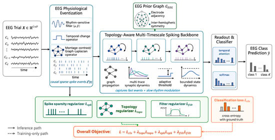
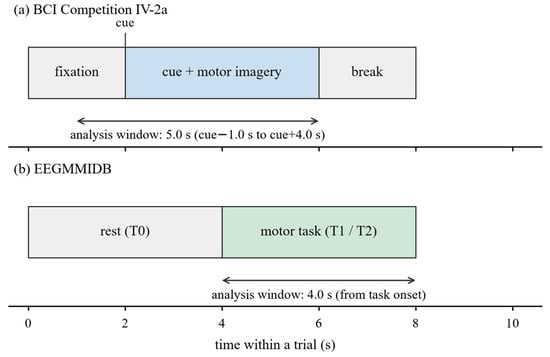
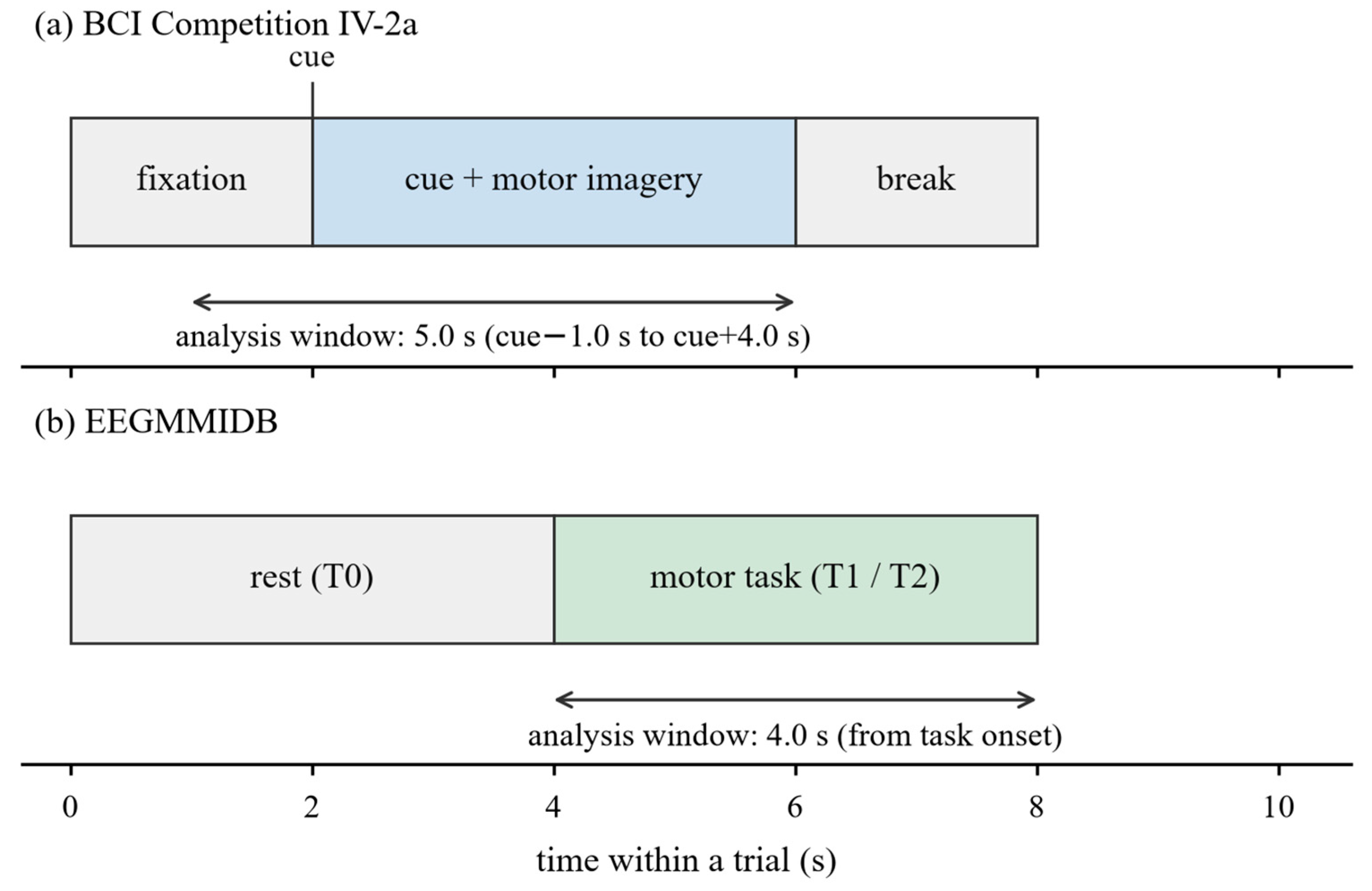
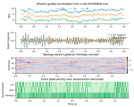
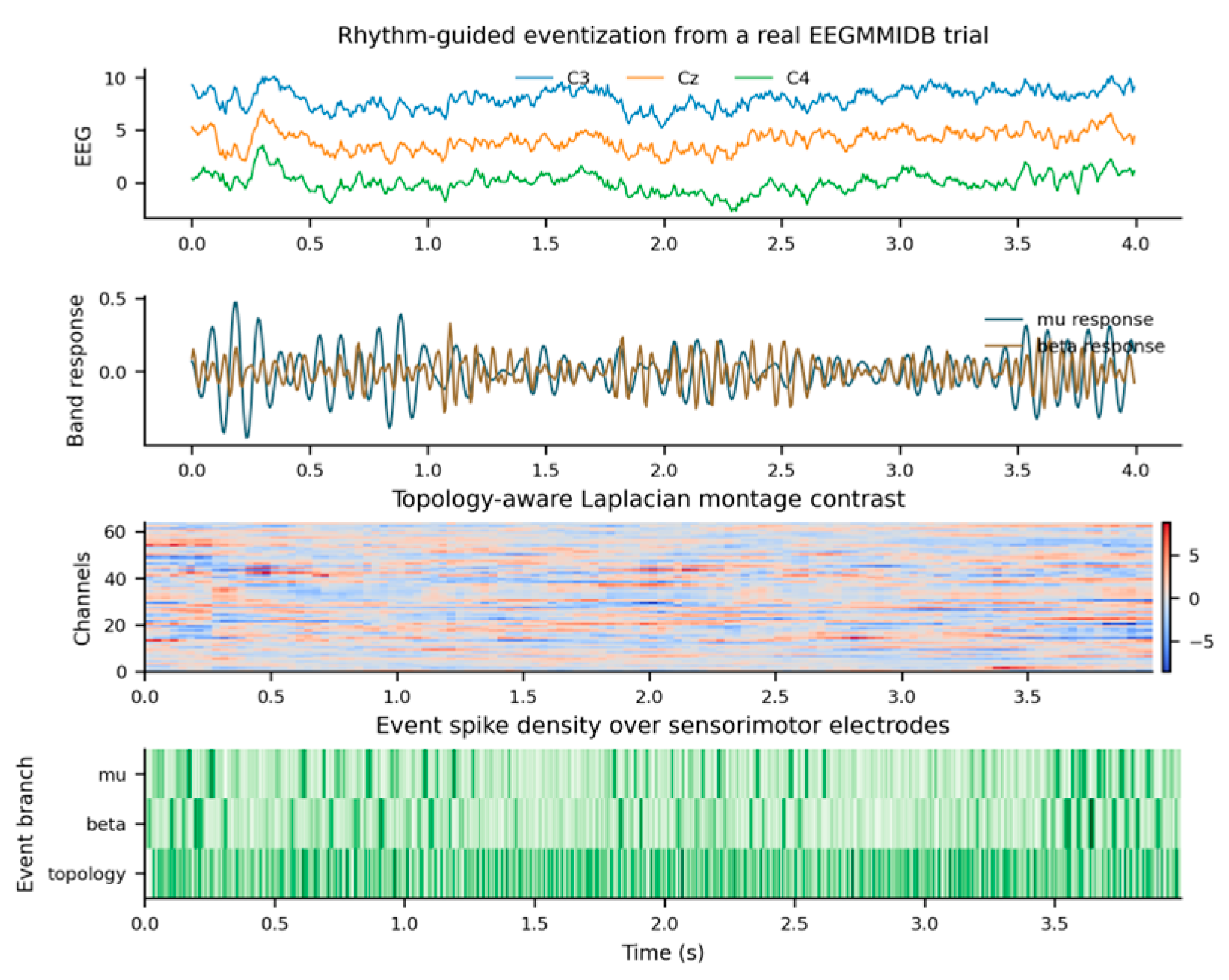
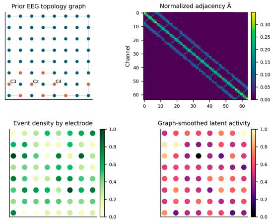
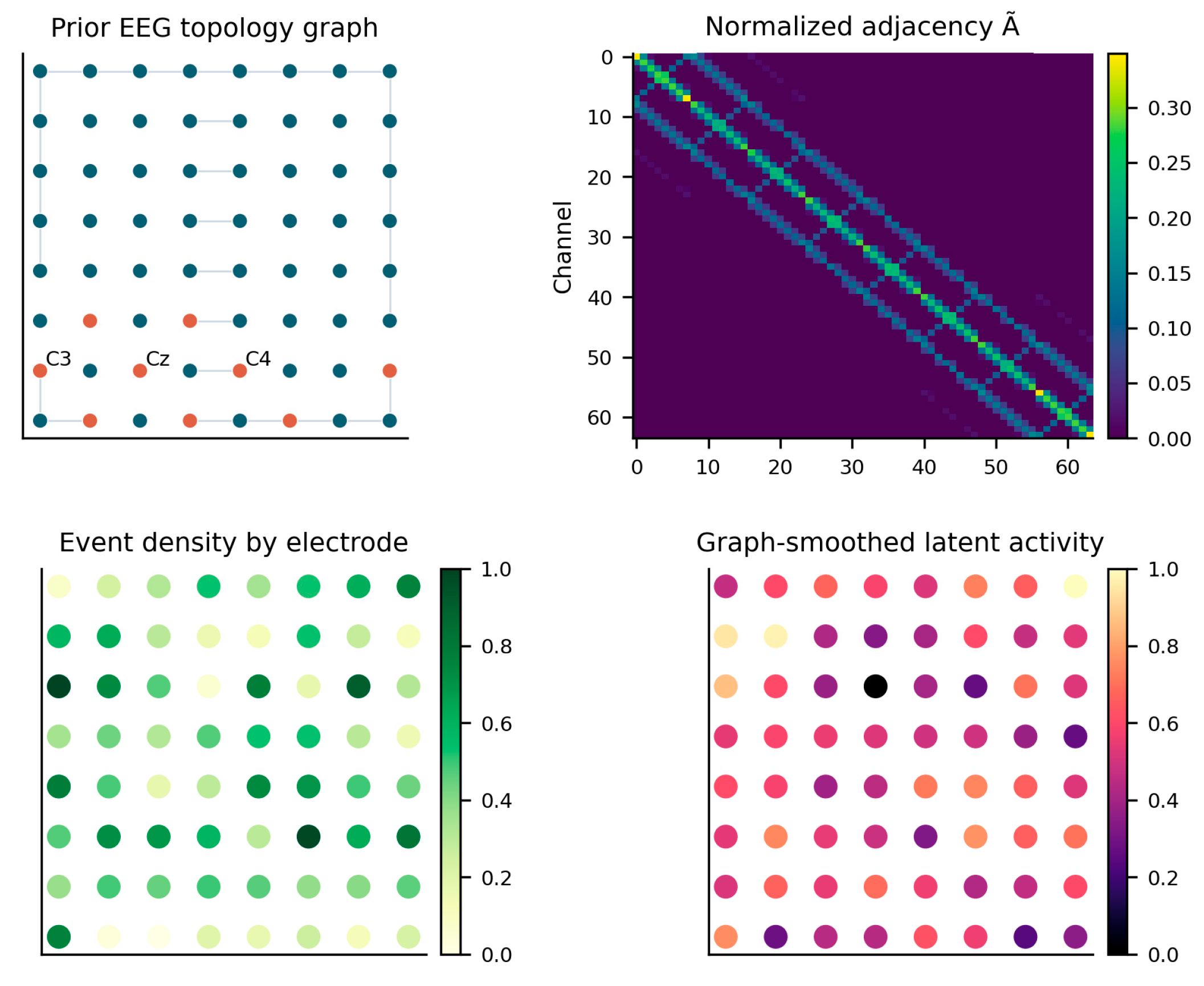
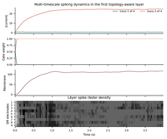
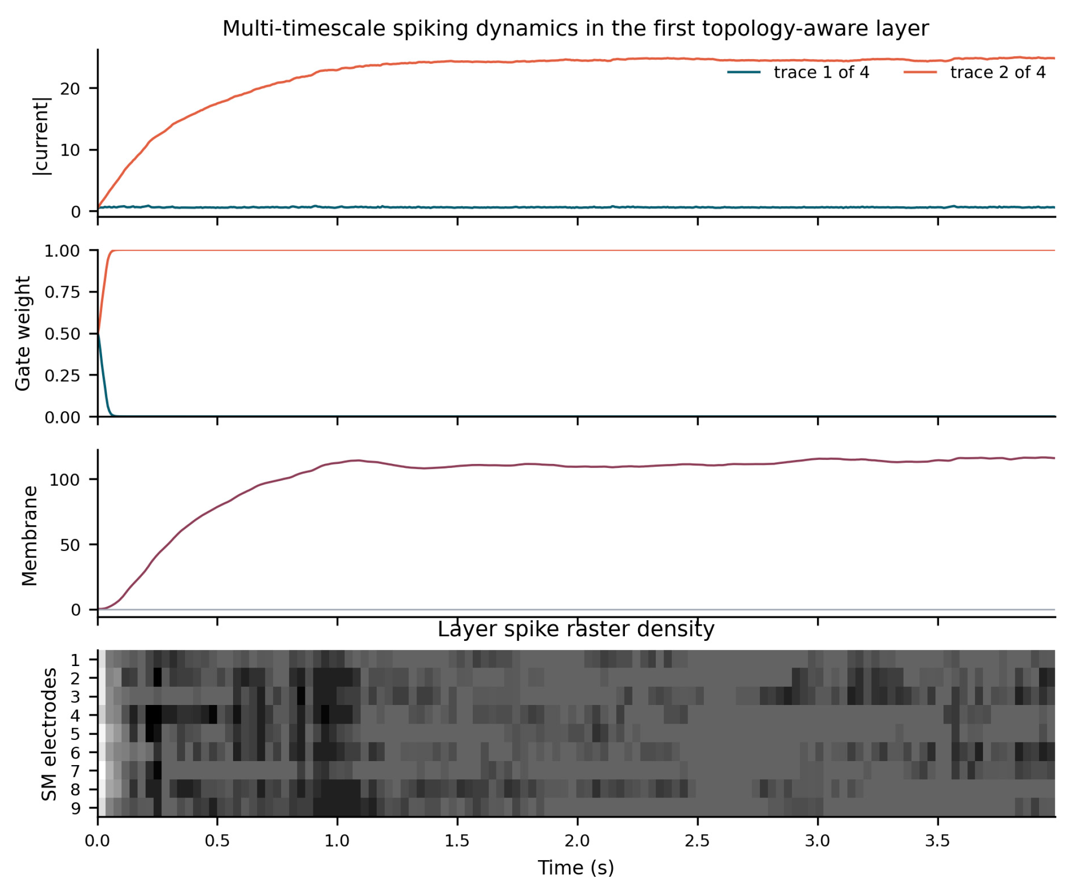
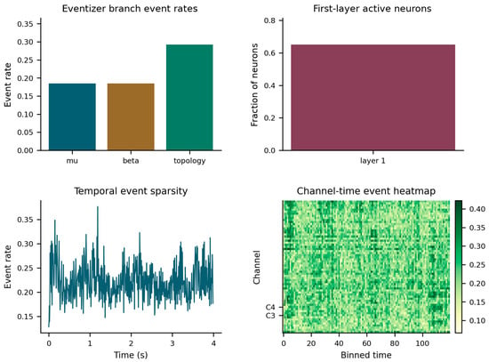
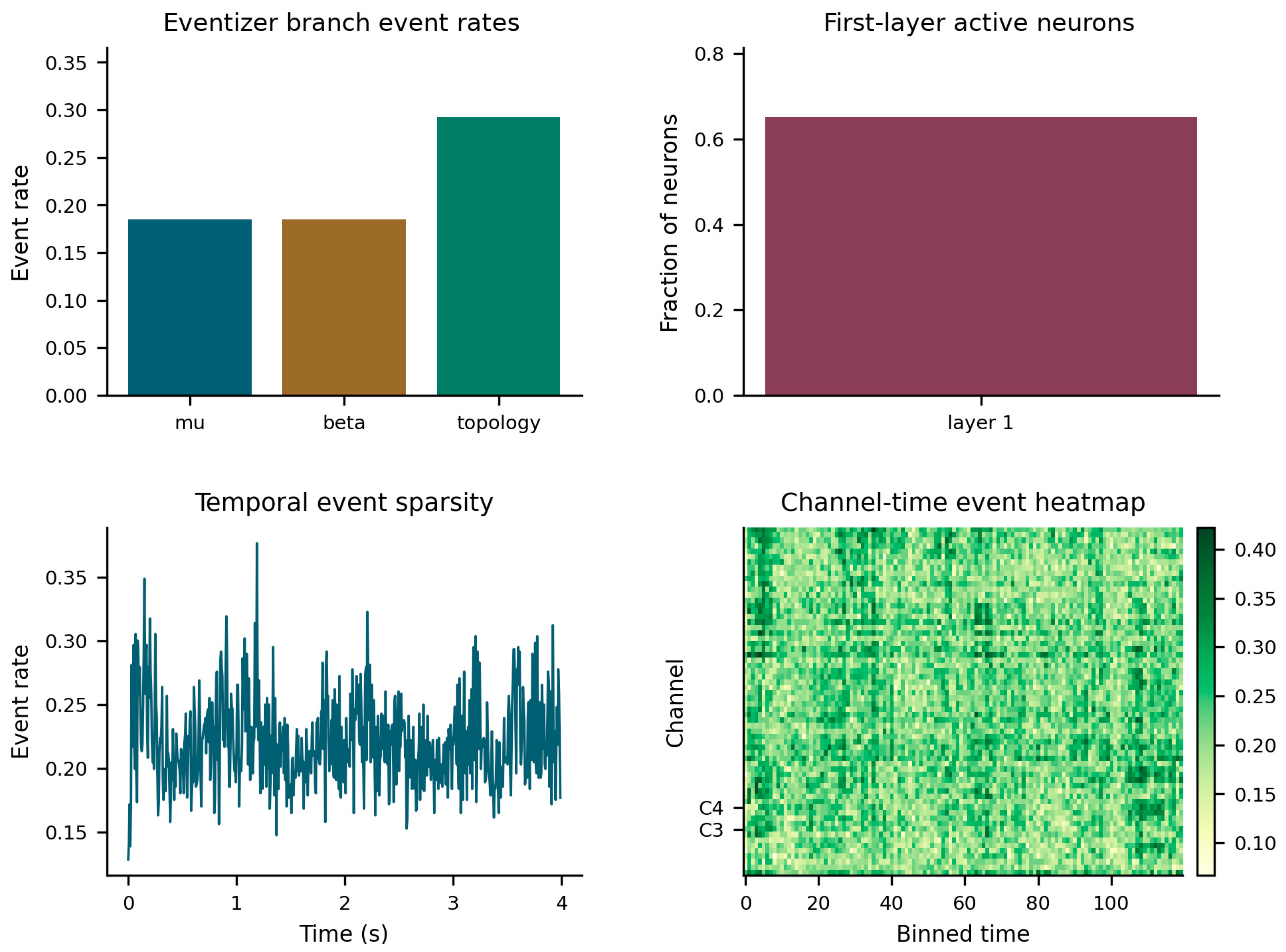

Disclaimer/Publisher’s Note: The statements, opinions and data contained in all publications are solely those of the individual author(s) and contributor(s) and not of MDPI and/or the editor(s). MDPI and/or the editor(s) disclaim responsibility for any injury to people or property resulting from any ideas, methods, instructions or products referred to in the content. |
© 2026 by the authors. Licensee MDPI, Basel, Switzerland. This article is an open access article distributed under the terms and conditions of the Creative Commons Attribution (CC BY) license.