


Highlights
What are the main findings?
- Under the All configuration, incremental factor graph optimization (FGO) has a lower mean score than an extended Kalman filter (EKF) but wins only 29 of 59 sessions.
- Removing time-differenced carrier phase from All improves EKF but worsens FGO, including when both use the same acceptance rule and uncertainty.
What are the implications of the main findings?
- Matched-input comparisons must distinguish estimator-specific screening, weighting, and state handling.
- Tail failures and sensitivity to output-support exclusions can reverse aggregate estimator rankings.
Abstract
This study compares an extended Kalman filter (EKF) and incremental factor graph optimization (FGO) for smartphone carrier-phase differential global navigation satellite system (GNSS) positioning with float ambiguities. Both receive identical physical observation candidates from a common front end but retain distinct state parameterizations, screening, weighting, ambiguity handling, and update procedures. Forward-only offline replay uses measurements available up to each epoch without revising previous outputs. Twelve auxiliary-observation configurations are evaluated across 154 route–phone pairs and 59 equally weighted driving sessions. Under Base, FGO has a higher mean Google Smartphone Decimeter Challenge score than EKF (3.600 versus 2.825 m). Combining all auxiliary observations (All) reduces the FGO mean score by 8.4% relative to EKF (2.622 versus 2.864 m), but this advantage comes from a few influential sessions: FGO wins only 29 of 59 sessions, and the exploratory 95% confidence interval of the paired mean difference (−1.427 to +0.599 m) includes zero. Removing time-differenced carrier phase (TDCP) from All improves EKF but worsens FGO, and this opposite response strengthens when both estimators use the same TDCP acceptance rule and uncertainty. Including a separately reported case with asymmetric estimator-output support reverses the All ranking. The results characterize the tested implementations, not general FGO superiority.
1. Introduction
Modern smartphones can provide raw global navigation satellite system (GNSS) pseudorange, carrier-phase, and Doppler observations, allowing high-precision positioning methods originally developed for survey-grade receivers to be extended to consumer devices. Compared with survey-grade equipment, smartphones are more strongly affected by compact antennas, handset blockage, lower carrier-to-noise density ratios, multipath, and non-line-of-sight propagation, and are particularly prone to carrier-phase cycle slips and continuity interruptions. Previous studies have shown that dual-frequency smartphones have the potential to support single-baseline real-time kinematic (RTK) and centimeter- to decimeter-level positioning, while also revealing substantial measurement-quality differences across devices and environments [1,2].
The Google Smartphone Decimeter Challenge (GSDC) [3] has accelerated research on high-precision positioning using raw smartphone GNSS and inertial measurements. Suzuki investigated global position–velocity optimization using factor graph optimization (FGO), two-step optimization based on carrier-phase observations, and GNSS/inertial measurement unit (IMU) factor-graph integration [4,5,6]. Zhong et al. used robust optimization to mitigate outliers in smartphone positioning [7], Jiang et al. combined FGO with solution separation [8], Geng et al. studied an FGO implementation for Android GNSS RTK [9], and Wang et al. examined multi-GNSS RTK FGO in urban environments [10]. Unified probabilistic modeling with factor graphs and incremental inference with iSAM2 provide the theoretical and computational basis for multi-epoch state estimation [11,12], and incremental smoothing has also been applied to GNSS-aided inertial navigation [13]. Ng et al. introduced differential GNSS (DGNSS)-corrected pseudorange and time-differenced carrier phase (TDCP) measurements into differentiable FGO [14], while Motooka investigated tightly coupled GNSS/inertial navigation system (INS) integration for smartphone positioning [15]. Wen et al. directly compared the extended Kalman filter (EKF) and FGO for loosely and tightly coupled GNSS/INS integration in an urban canyon and attributed the advantage of FGO mainly to its multiple iterations and to the larger amount of historical data used in the optimization [16]. Song et al. showed that a sliding-window FGO with a single-state window and suitable marginalization reduces to the iterated EKF, and that larger windows do not necessarily improve accuracy [17]. Both studies used vehicle-mounted receivers, pseudorange measurements, and a dedicated IMU with its own attitude solution, unlike smartphone carrier-phase positioning with its frequent interruptions and unknown phone attitude.
These studies demonstrate the flexibility of FGO for integrating heterogeneous observations. Direct comparisons between EKF and FGO [16,17,18], FGO formulations that combine pseudorange with Doppler, TDCP, or inertial information [4,5,6,14], and tightly coupled GNSS/INS integration [15] have also been reported; the novelty of the present study therefore lies neither in comparing EKF and FGO nor in applying FGO to smartphone GNSS but in a controlled, quantitative comparison of the two estimators on a large set of smartphone recordings. However, front-end preprocessing, measurement screening, weighting, smoothing strategy, state definition, and sensor models often change simultaneously across different studies. Consequently, an observed performance difference cannot necessarily be attributed to the optimization framework alone. This issue is particularly important for smartphone carrier-phase differential positioning because Doppler, TDCP, inertial motion constraints, and zero-velocity updates (ZUPT) provide different forms of motion information which are handled differently by recursive filtering and graph optimization.
To reduce these confounding effects, rover GNSS, base-station GNSS, broadcast ephemerides, and smartphone IMU data are first processed by a common front end that performs time alignment, satellite-state computation, signal pairing, double-difference (DD) construction, and carrier-phase continuity management. The same preprocessed observation candidates are then supplied to the EKF and incremental FGO. After the estimator split, the two methods retain their own state parameterizations, measurement screening, weighting, ambiguity handling, and update procedures and do not exchange estimates or internal decisions. The experiments use offline replay under a strictly forward information boundary: the estimate at epoch k uses only measurements available up to epoch k, and previously published positions are not revised by backward smoothing or end-of-route re-estimation. The comparison is therefore matched in its observation inputs and information boundary but not in the measurement screening, weighting, and state handling of the two estimators; these estimator-specific differences are stated explicitly in Section 2.
Under this matched setting, twelve configurations are compared: Base; Doppler, TDCP, an IMU-based lateral-motion constraint (IMU-LC), and ZUPT alone; the combinations IMU-LC+ZUPT, Doppler+TDCP, and All; and All with one observation removed at a time, which shows the contribution of each observation within All. The analysis focuses on three questions: whether individual auxiliary observations affect the two estimators in the same way; whether combining multiple sources of auxiliary information improves both typical and high-percentile errors; and whether an improvement in the aggregate mean implies consistent improvement across most driving sessions.
Rather than proposing a new RTK or FGO positioning method, this work provides a controlled, matched comparison whose purpose is to determine whether, and under which auxiliary-observation configurations, the incremental FGO implementation tested here provides an advantage over the tested EKF implementation when measurement generation and preprocessing are kept as consistent as possible. Its main contributions are as follows. First, a strictly forward matched-input EKF-FGO comparison is established under a common front end so that both estimators use the same physical observation candidates while remaining independent after the estimator split. The estimator-specific screening, weighting, and state handling that remain are listed explicitly, and the influence of the DD weighting and of the TDCP acceptance rule and uncertainty is examined with controlled setting changes. Second, twelve auxiliary-observation configurations are evaluated on 154 route–phone pairs from 59 driving sessions. In the tested implementations, representing the same float-ambiguity DD observations in an incremental graph gives no advantage under Base. A clear mean FGO advantage appears only when Doppler, TDCP, and IMU-LC are combined. In addition, TDCP acts in opposite directions in the two estimators, even when both use the same TDCP acceptance rule and nominal uncertainty. Earlier comparisons attributed the advantage of FGO mainly to multiple iterations and a longer measurement history [16] or found that larger windows do not necessarily improve accuracy [17]. In contrast, in the present smartphone carrier-phase setting, the strictly forward FGO gives no advantage on the same float-ambiguity DD observations. Its advantage depends on which auxiliary observations are combined and on how each estimator represents cross-epoch information. Third, the aggregate comparison is examined at the session level with medians, trimmed means, leave-one-session-out ranges, and within-session difference-in-differences, and accuracy is separated from output availability. These analyses show that the mean FGO advantage under All is carried by a few high-impact sessions. The conclusions therefore concern the tested implementations and settings, not EKF and FGO in general.
2. System Model and Estimation Methods
2.1. Common Forward Observation Processing
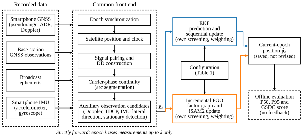
The system inputs are rover GNSS observations, base-station GNSS observations, broadcast ephemerides, and smartphone IMU measurements. To keep the physical observation inputs identical for EKF and FGO, epoch synchronization, satellite position and clock computation, signal pairing, single- and double-difference construction, carrier-phase continuity checking, and auxiliary-observation candidate generation are completed before entering either estimator. Both estimators receive the same candidate observations, reference satellites, and carrier-phase arc segmentation. Measurement gating, weighting, ambiguity handling, and state updating are then performed independently by EKF and FGO, so the finally accepted measurements and their effective weights can differ between the two estimators. The comparison is therefore between two complete estimator architectures under matched physical observation inputs rather than a solver-only substitution. Here, “matched” refers to the observation candidates, front-end processing, causal information boundary, and evaluation; measurement screening and weighting remain estimator specific and are summarized in Section 2.6. The overall processing flow is shown in Figure 1.
Figure 1.
Overall processing flow. The common front end provides the same observation candidates to both estimators; EKF and incremental FGO then process them independently under the configuration selected in Table 1, and each current-epoch position is saved without later revision and used only for offline evaluation.
Let r and b denote the rover and base station, respectively; q denotes the reference satellite; and s denotes a target satellite. The common front end selects the reference satellite separately for each constellation, frequency band, and observation type (pseudorange or carrier phase) as the satellite with the highest elevation. For , the rover-minus-base single-difference observation-minus-model residuals are
Table 1.
Observation configurations.
In each line of (1), the first parenthesized term is the rover observation minus its model and the second is the corresponding base-station term. P is pseudorange in meters, is the carrier phase in cycles, and is the corresponding wavelength, so is in meters. The vectors and are the rover Earth-centered, Earth-fixed (ECEF) position and the known base-station ECEF position, respectively. In this implementation, code and phase share the modeled range h, which includes geometric range and the applied Sagnac, satellite-clock, and hydrostatic-troposphere corrections but excludes ambiguities. For base-station quantities, k labels the latest base observation whose timestamp is not later than rover epoch k. Observations older than 30 s are not used, and base observations are not interpolated in time. The base-station data used in this study are sampled every 30 s, so the age of the base observation varies between 0 and 30 s, with a mean of 15 s (Table S7). The satellite positions and clocks for the base observation are computed at its own timestamp. However, errors that change between the two timestamps, such as atmospheric delays and broadcast satellite-clock errors, do not cancel completely in the DD residuals. TDCP is formed only when both of its epochs use the same base observation. Only GPS, Galileo, and GLONASS signals in the L1/E1 and L5/E5a bands are used. Each signal must have pseudorange at both receivers, an elevation of at least at both receivers, and a rover carrier-to-noise density ratio () of at least 28 dB-Hz (L1/E1) or 20 dB-Hz (L5/E5a). An epoch without a base observation within 30 s has no DD observations; in the primary cohort, every epoch had one. The hydrostatic tropospheric delay is modeled at both receivers, whereas the differential wet tropospheric and ionospheric delays are not modeled. These delays enter the DD residuals, where the slowly varying part of their carrier-phase effect may be partly absorbed by the float ambiguities. The variance model contains no baseline-dependent term (Appendix A). The real-valued rover–base single-difference float ambiguity, in cycles, is
Here, and denote the receiver-specific ambiguity terms. Only their single difference is estimated, rather than the two receiver ambiguities separately. Using a reference-minus-target DD convention, the DD pseudorange and carrier-phase residuals are written as [19,20]
In (3), the leading r denotes a residual, whereas the receiver subscript r denotes the rover; the base-station contribution is already included in and . The phase single difference retains its ambiguity term, whose double-difference contribution is subtracted in (3).
Both estimators estimate these float ambiguities explicitly in every configuration, including Base, so the carrier phase enters both estimators directly through the DD carrier-phase observations, not only through TDCP. Integer ambiguity resolution is not performed. An ambiguity state remains active while the carrier-phase arc is continuous; a new arc is created after a cycle slip, observation interruption, reacquisition, or other continuity failure. The common front end fixes the candidate identity, reference satellite, and continuity information but not the observation geometry at a single initial position. Therefore, both EKF and FGO re-evaluate the physical observation model using their own current states. The activation and reinitialization of ambiguity states within each estimator also depend on its own measurement acceptance and reset logic. The ambiguity bookkeeping of the two estimators, including initialization, reference-satellite changes, retirement, and recovery, is summarized in Appendix B.
2.2. Extended Kalman Filter Estimation
The EKF follows a recursive predict–update structure [21]. Its state contains the ECEF position, velocity, acceleration, and float ambiguities associated with the currently active carrier-phase arcs:
where , , and are the three-dimensional position, velocity, and acceleration, respectively, and is the set of currently active float ambiguities. No additional ionospheric state is used. The navigation state is propagated forward using a position–velocity–acceleration model, whose main relations are
To avoid an overly strong acceleration constraint when the position uncertainty is large, the second-order acceleration-to-position term is used only when the mean of the three position variances is below 0.25 m2. Equation (5) therefore represents the principal EKF motion-propagation model. For any measurement that passes the EKF measurement check, let be the innovation and the measurement Jacobian. The standard extended Kalman update is then
DD pseudorange primarily constrains position, whereas the DD carrier phase constrains both position and float ambiguities. The DD update of the EKF follows the relative-positioning routine of RTKLIB [22] in its demo5 version, including its correlated DD covariance and single-difference variance model (Appendix A). Its settings were adapted from those proposed for smartphone measurements [23]. Within each epoch, the EKF first applies one batch update with the DD pseudorange and carrier phase and then sequential updates with Doppler, TDCP, ZUPT, and IMU-LC. TDCP and IMU-LC relate the current position to the previously published position. The EKF does not augment its state with that position; instead, it treats the previous position as a known value and adds the projection of its marginal covariance to the measurement variance. The cross-covariance between the current and previous states is thus neglected (Appendix A). Although EKF and FGO use the same candidate observations and the same physical measurement definitions, their measurement gating, weighting, and state responses are computed independently.
2.3. Incremental Factor Graph Optimization
The incremental FGO uses the position , velocity , and float ambiguities associated with valid carrier-phase arcs as its main variables at each epoch. The variable set up to epoch k is denoted by
where denotes the set of float-ambiguity variables maintained in the graph up to the current epoch. The two estimators do not employ identical state parameterizations: unlike the EKF, the FGO does not optimize an explicit acceleration state, and acceleration effects are represented stochastically through the process uncertainty of the temporal factors. The two motion models are therefore not assumed to be stochastically equivalent, and this difference may itself contribute to the observed performance difference. The IMU aiding used in this study is not a full GNSS/INS formulation; therefore, the graph state does not include a complete inertial state such as attitude, accelerometer bias, or gyroscope bias.
Given the factor set that has arrived by the current epoch, the state estimate is obtained by robust weighted nonlinear least squares [11,24]:
where is the factor residual, is the corresponding covariance, and is a robust loss used when required. The estimate covers all variables in , but only the current-epoch position is published. Incremental inference is performed with iSAM2 [12]. The DD pseudorange and carrier-phase factors use the physical model in (3), and their observation geometry is re-evaluated from the current graph variables whenever linearization or relinearization is required, rather than being fixed at a linearization around the initial position. The resulting graph and the factor types used in this study are shown in Figure 2.
Figure 2.
Incremental factor graph when epoch k is processed. White circles denote the position–velocity state of each epoch, and gray circles N denote the single-difference float ambiguities of a continuous carrier-phase arc, which are shared by the DD carrier-phase factors of all epochs in that arc. Squares denote factors, labeled by type in the superscript and by epoch in the subscript: 0, initialization or recovery prior (Equation (19)); MM, motion model (Equations (9) and (10)); TDCP, time-differenced carrier phase connecting the positions of two adjacent epochs (Equation (12)); LAT, IMU-LC lateral constraint connecting the same two positions (Equation (16)); P, DD pseudorange, and , DD carrier phase, which also connects the ambiguity nodes of its arc (Equation (3)); D, Doppler, acting on the position and velocity of one epoch (Equation (11)); Z, ZUPT on the velocity (Equation (18)). Only the new state and the factors in the shaded area are added at epoch k; historical variables may be relinearized, but previously published positions are not replaced.
Unlike the EKF, which explicitly retains acceleration states, the FGO represents short-term motion through probabilistic constraints between the position and velocity of adjacent epochs. The position–velocity motion factor and velocity random-walk factor used in this study are
where is the process-noise parameter (Table 2) and the corresponding standard deviations vary with the time interval, with lower bounds of 10−3 m and 10−3 m/s, respectively. Equations (9) and (10) together define the basic temporal-evolution model of the FGO. Whereas the EKF recursively compresses historical information into the current posterior mean and covariance, the FGO explicitly retains factor connections across epochs.
Table 2.
Principal estimator and auxiliary-constraint parameters.
2.4. Doppler, TDCP, IMU-LC, and ZUPT Aiding Constraints
The four auxiliary observations below are used by both estimators, as measurement or pseudo-measurement updates in the EKF and as factors in the FGO, with estimator-specific screening and weighting (Table 2). Doppler measurements reflect the satellite–receiver range rate and provide information on the current motion state [6,25,26]. For satellite i, let denote the velocity-type observation after carrier-wavelength and satellite-clock-drift correction. The Doppler innovation between reference satellite q and target satellite s is
Here, D, , , and are the rover Doppler measurement in Hz, the carrier wavelength, the satellite clock drift in m/s, and the predicted range rate; the receiver clock drift cancels in the between-satellite difference. Because the range-rate geometry depends on both the current position and velocity, Doppler is not treated as a pure velocity observation in this study. The EKF uses it as a current-epoch measurement update, whereas the FGO represents the same physical information as a factor involving and . In each epoch, all Doppler differences share one reference satellite, the one with the highest elevation. The EKF excludes differences that involve a GLONASS satellite because including them worsened its score during development (Section 2.6), whereas the FGO uses all candidates. Of the 15.8 candidate differences per epoch, 35% involve a GLONASS satellite, and in 11.7% of the epochs the reference satellite itself is a GLONASS satellite, so the EKF uses no Doppler in those epochs. Under All, the EKF and the FGO used 10.2 and 15.8 Doppler differences per epoch, respectively (Table S3).
TDCP exploits the fact that the ambiguity remains constant over a continuous carrier-phase arc and obtains precise relative-motion information through temporal differencing [5,14,27]. Using the single-difference quantities defined in (1), it is formed as the current-epoch DD quantity minus the previous-epoch DD quantity:
TDCP is used only when the reference satellite, target satellite, carrier-phase arcs, and temporal association remain continuous. The ambiguity terms shared by both epochs of these continuous arcs then cancel, so (12) depends only on and , not on the estimated float ambiguities. In the EKF, the previously published position and its uncertainty enter the current sequential update as historical information. In the FGO, TDCP directly forms a cross-epoch factor connecting and . Thus, both estimators use the same physical TDCP information but represent the historical information differently. The acceptance rule and the measurement uncertainty of TDCP are also estimator specific (Section 2.6): whenever the EKF solution is in its float state, the EKF uses TDCP only for satellite pairs in which at least one ambiguity is newly initialized, whereas the FGO applies no such restriction. The same TDCP candidates therefore do not guarantee that the same TDCP information is accepted by both estimators. A TDCP observation is the exact time difference of two DD carrier-phase observations, which may also be used in their own DD updates. Its errors are therefore correlated with those observations and with the adjacent TDCP observation of the same pair. Neither estimator models this correlation; the FGO uses an independence approximation and treats each TDCP factor and each DD carrier-phase factor as independent. The EKF does not model the correlation either, but in the float state its acceptance rule uses only pairs in which at least one ambiguity has just been initialized. TDCP is then used mainly when the DD carrier-phase information of the current epoch has been absorbed by a re-initialized ambiguity, and the eightfold standard deviation further down-weights the remaining rows. In a linear Gaussian example (Appendix C), using the DD carrier phase and its exact time difference with their full joint covariance gives the same estimate and covariance as the DD carrier phase alone. Treating the two as independent leaves the estimate practically unchanged in that example but makes the nominal uncertainty too small. Because the real estimators screen measurements, use robust losses, and re-initialize ambiguities, this idealized result does not predict their behavior. The effect of matching the TDCP acceptance rule and uncertainty is examined in Section 4.3.
The IMU-LC configuration in this work is not a full GNSS/INS mechanization. Conventional GNSS/IMU integration also estimates attitude and inertial-sensor biases, by strapdown mechanization in an EKF [28] or by preintegrated IMU factors in an FGO [13,29], which requires the attitude of a smartphone whose mounting in the vehicle is unknown. IMU-LC, the IMU-based lateral-motion constraint, instead combines the heading change measured by the gyroscope with the land-vehicle constraint that the vehicle does not move sideways [30]; the accelerometer only gives the direction of gravity. No attitude or bias state is therefore needed, and both estimators keep the states of the GNSS-only configurations. The front end estimates the gravity direction as the normalized mean of all accelerometer samples received up to . It then integrates the angular rate about this direction over the epoch interval with the trapezoidal rule, using only samples received by :
Because the mounting of the phone is unknown, each estimator calibrates the sign and the rate bias of this yaw change online against the change of its own velocity heading . The calibration is cumulative rather than windowed. The set contains all epoch pairs since the start of the route and before epoch k that meet three conditions: both epochs are in the float state with horizontal speeds of at least 3 m/s, the interval is at most 2.5 s, and rad. From these pairs, the sign, the rate bias, and the calibrated yaw increment are obtained as
The calibrated increment is used only after 50 pairs have been collected. The heading is propagated with it and re-anchored to the velocity heading at float-state epochs with speeds of at least 3 m/s:
where wrap(·) maps an angle to ; at other epochs, . The heading chain is restarted when the calibrated yaw increment is unavailable or the epoch interval exceeds 10 s, and it is re-initialized with at the next anchoring epoch. Let be the heading at the middle of the epoch interval and the horizontal unit vector perpendicular to it. Here, and are the east and north unit vectors at the first estimated position of the route, expressed in ECEF coordinates and kept fixed for the route; the velocity heading is computed in the same frame. The lateral-motion residual is
To suppress the cross-track jumps caused by multipath and carrier-phase disruptions, the constraint is applied only at transient epochs, that is, when the solution is not in its float state (fewer than four satellites with accepted L1 carrier phase), four or more DD measurements are rejected, or the median absolute DD carrier-phase residual exceeds 0.05 m. In addition, the epoch interval must be at most 2.5 s, the speed at the previous epoch at least 3 m/s, and the yaw calibration complete. The position standard deviation along must also be at most 5 m; the EKF evaluates it from its current state before the constraint, whereas the FGO uses the marginal covariance of the previous position. The FGO further requires that its heading has been re-anchored within the last 10 s. The two estimators evaluate the transient test at different points: the EKF adds the rejections before and after its DD update, so a measurement rejected in both counts twice, and it uses the carrier-phase residuals after the update. The FGO uses the rejections and carrier-phase residuals of its gating at the predicted state before the graph update. The two estimators therefore classify epochs differently: under All, IMU-LC was applied at 23% of the epochs in the EKF and at 65% in the FGO (Table S3). The EKF applies the constraint as a pseudo-measurement in the sequential update, whereas the FGO uses it as a factor with a Huber loss connecting two adjacent position nodes. In the EKF, the projected covariance of the previous position is added to the variance, and the variance is inflated according to the innovation (Appendix A).
Against the ground truth, the calibrated yaw increment had a median absolute error of 0. per epoch on straight segments, with a 95th percentile of 0. (Table S3). In turns faster than /s, the median error was 0. to 0. and the 95th percentile 2. to 2.. The online calibration estimates only a sign and a rate bias, not a scale factor, which may explain the larger errors in turns. The direction of the constraint is least reliable in turns: even with the heading chain anchored to the ground-truth course, it differed from the ground-truth step direction by a median of 0. at 5–15∘/s and 1. above /s. These differences correspond to cross-track offsets of 0.14 and 0.24 m over one epoch, whereas the nominal standard deviations are 0.03 m in the EKF and 0.30 m in the FGO.
Stationary updates are an established aid for land-vehicle inertial navigation [31]; here, stops are detected with a variance-type detector [32]. For the accelerometer samples received in , the detection statistic is
and is computed in the same way from the gyroscope samples; at least 20 samples of each sensor are required. Because the statistics use magnitudes, they are insensitive to constant sensor biases and to the unknown phone attitude. Epoch k is regarded as stationary when m/s2, rad/s, and the horizontal speed estimated by the respective estimator is below 0.7 m/s (Table 2). For this speed, the EKF uses its current state before the IMU-based updates, whereas the FGO uses its estimate at the previous epoch. The two thresholds lie between the vibration levels measured on three development routes. During stops, including engine idling, m/s2 and rad/s, whereas during driving m/s2 and rad/s. The speed condition prevents false detections during smooth constant-speed driving, which is also vibration-quiet. As a consequence, ZUPT is not triggered while the estimated speed is grossly wrong. A three-dimensional zero-velocity constraint is then applied:
Accordingly, the IMU-LC and ZUPT configurations in this study provide only vehicle-motion-direction and stationary information. ZUPT constrains only the three-dimensional velocity and does not additionally fix the position.
Under All, ZUPT was applied at 18.4% and 18.6% of the epochs in the EKF and the FGO, respectively, on average over the route–phone pairs, compared with 20.0% of the epochs whose ground-truth speed was below 0.2 m/s. Across pairs, the ZUPT fraction and the ground-truth stationary fraction had a correlation of 0.98 for both estimators (Table S3). Because per-epoch ZUPT flags were not stored, the detector was also evaluated epoch by epoch with the vibration statistics stored by the front end and with the ground-truth speed in place of the estimated speed (Table S3). This evaluation describes the detector when the speed is correct. Here, an epoch is regarded as stationary when the ground-truth speed is below 0.2 m/s at both ends of the interval. The vibration criterion held in 92.9% of the stationary epochs, in 94.7% of the epochs within stops and in 70.4% at their first and last epochs. It also held in 2.1% of the moving epochs. These false detections occurred mainly at low speed, in 42.8% of the epochs between 0.2 and 0.7 m/s and in 21.4% of those between 0.7 and 3 m/s outside turns. Above 3 m/s, they occurred in at most 0.3% of the epochs, on straight roads as well as in turns. With a correct speed, the 0.7 m/s gate removes every detection above 3 m/s. False detections then remain in 0.9% of the moving epochs, all with a speed below 0.7 m/s at the end of the interval.
2.5. Initialization, Recovery, and Strictly Forward Updating
At the first valid epoch or when the graph state must be re-established, the incremental FGO uses the currently available position and velocity from the common front end to form initialization/recovery priors (Appendix B). After a long observation interruption, the graph may instead be restarted from its own prediction and the previous velocity. In both cases, the priors are as follows, where the tilde marks the prior position and velocity:
Figure 2 shows the incremental factor graph from the first epoch to the current epoch k. Historical position and velocity propagate to the current epoch through motion factors; TDCP and the IMU-LC lateral constraint connect states across epochs; and Doppler, DD GNSS, and ZUPT act on the current epoch. When a new epoch arrives, only the new variables and factors are added. After one iSAM2 incremental update, the current-epoch position is read out immediately. Historical variables may continue to participate in subsequent inference, but previously published positions are not recomputed at the end of the route using future measurements. In the replay, base-station observations and IMU samples are used only up to the measurement time of the current epoch; actual message-arrival delays are not simulated, and each broadcast ephemeris is treated as available from its reference time. The replay is therefore not an end-to-end real-time validation.
2.6. Observation Configurations
Twelve auxiliary-observation configurations are constructed under the same front-end observation conditions. Base uses only DD pseudorange and DD carrier phase with float ambiguities; the remaining configurations add one or more auxiliary observations. They comprise Doppler, TDCP, IMU-LC, and ZUPT alone, where ZUPT uses the IMU data only for stationary detection; the combinations IMU-LC+ZUPT, Doppler+TDCP, and All; and the four configurations obtained by removing exactly one of Doppler, TDCP, IMU-LC, and ZUPT from All (All−Doppler, All−TDCP, Doppler+TDCP+ZUPT, and Doppler+TDCP+IMU-LC, respectively). Removing Doppler disables only the EKF Doppler update and the FGO Doppler factor; the Doppler information already used by the common front end, for example for initialization, is unchanged. The twelve configurations, summarized in Table 1, do not form a full factorial design. No additional ionospheric state is enabled in any configuration.
The principal estimator and auxiliary-constraint parameters used in the experiments are summarized in Table 2. Parameters that differ between EKF and FGO are retained as part of their respective estimator architectures rather than being forced to have identical internal settings. Even where the nominal constants are equal, the effective weights can differ: for IMU-LC and TDCP, the EKF additionally includes the projected uncertainty of the previous position and inflates the variance according to the innovation, whereas the FGO connects two position variables through a factor with a Huber loss.
All parameters were fixed during development, before the evaluation runs, and were not changed afterwards. The EKF was first implemented as a port of the RTKLIB relative-positioning routine (Section 2.2). The auxiliary constraints and the FGO-specific settings were then set separately for each estimator by changing one parameter at a time and comparing the mean GSDC score of the Pixel 6 Pro recordings of 14 development routes; the recordings of the other 19 device models were not used for tuning. Table S2 lists the values tried and the resulting scores. These 14 routes belong to the 64 evaluated routes and cover 39 of the 154 route–phone pairs and 14 of the 59 driving sessions, including S53 and S58. The evaluation is therefore not independent of the development data, and the results for the remaining 45 sessions are reported separately in Section 4.4. The development record also explains two settings that differ between the estimators. First, the IMU-LC standard deviations of 0.03 m in the EKF and 0.30 m in the FGO do not have the same meaning. In the EKF, 0.03 m is only the nominal part of the variance, to which the projected previous-position variance and the innovation-based inflation are added; under All, 82% of the applied EKF IMU-LC updates were inflated (Table S3). In the FGO, the previous position is itself a variable, and 0.30 m is the full standard deviation of a factor that remains in the graph and is relinearized repeatedly. On the development routes, 0.03 m worsened the FGO score from 1.720 m to 1.879 m, whereas values from 0.1 to 0.5 m differed by less than 0.01 m. Second, the EKF TDCP acceptance rule and eightfold standard deviation were introduced because, when all pairs were accepted, the EKF covariance collapsed and one development route locked onto a biased solution. Section 4.3 repeats the TDCP-related configurations with both estimators using the same TDCP rule.
3. Experimental Setup and Evaluation Protocol
3.1. Dataset and Primary Analysis Cohort
The experiments use the public GSDC 2023–2024 training data. The selected recordings were collected on real roads in California, predominantly in the San Francisco Bay Area, including San Jose and Mountain View, with a smaller subset from the Los Angeles area. A record from one route and one smartphone is treated as a route–phone pair. The smartphones were made by Google (Mountain View, CA, USA), Samsung (Suwon, Republic of Korea), and Xiaomi (Beijing, China). The original dataset contains 156 such pairs. Temporal support after the common front-end processing is first examined: each pair is required to have at least half as many front-end epochs as ground-truth epochs, with fewer than 5% of its ground-truth epochs outside the time span of the front-end epochs. For 2020-08-04-00-19-us-ca-sb-mtv-101/Pixel 4, a relatively long ground-truth interval at the beginning of the trajectory has no corresponding position output; the first 286 of its 1690 ground-truth epochs (16.92%) precede the first front-end epoch. To prevent the score from being dominated by insufficient output coverage at the route start rather than by performance during valid positioning, this pair is not included in the primary cohort, reducing the cohort from 156 to 155 pairs. This criterion uses only the epoch times of the front-end output and the ground truth.
Among the remaining 155 pairs, 2023-09-06-00-01-us-ca-routen/SM-G955F exhibits uniquely severe estimator-output support asymmetry in every configuration. Under All, EKF provides 620 output epochs for 1650 ground-truth epochs (37.58%), whereas FGO provides 1630 (98.79%). It is the only remaining pair for which any EKF configuration has an output-support ratio below 50%, and the only pair with an EKF-FGO support asymmetry above 40 percentage points. Because the scorer aligns each estimator trajectory to all ground-truth epochs by interpolation and endpoint clamping, such a large support imbalance makes the resulting EKF-FGO score difference unsuitable for the primary accuracy comparison. This route–phone pair is therefore reported separately as a sensitivity case. Only this specific pair is excluded; the SM-G955F model as a whole and the remaining records of the same driving session are retained.
The resulting primary analysis contains 154 route–phone pairs from 64 routes while retaining all 59 driving sessions. The two exclusions address different comparability issues in the scoring protocol: the first concerns insufficient output coverage at the route start, whereas the second concerns severe asymmetry in estimator-output support. The second exclusion is motivated by scoring comparability, but its criterion was not specified independently of the accuracy results of this pair; the exclusion is therefore not accuracy-blind. The S53/SM-G955F pair is retained in full for the sensitivity analysis in Section 4.6, which also reports the effect of including it in the aggregate.
3.2. Driving Sessions and Equal-Weight Aggregation
The same physical drive may be recorded simultaneously by several smartphones. If all route–phone pairs were averaged directly with equal weight, driving sessions containing more phones would receive greater statistical weight. The records belonging to the same physical drive are therefore grouped into a driving session. Labels such as S49 and S53 are internal identifiers used only to identify driving sessions in figures and discussion; they do not denote algorithms, device categories, or experimental configurations.
For configuration c and estimator e, the metric is first computed independently for each route–phone pair and averaged over the phones recorded on the same route. Let the jth driving session contain routes, and let denote the phone-averaged metric of route m. The session-level metric is then
The 59 driving sessions are then assigned equal weight:
Thus, phones are weighted equally within a route, routes equally within a session, and the 59 driving sessions equally. The 50th- and 95th-percentile horizontal errors (P50 and P95) and the GSDC score reported in Section 4 are therefore equal-weight statistics over the 59 driving sessions, rather than percentiles recomputed after pooling all ground-truth epochs into a single global error distribution.
3.3. Time Alignment, Endpoint Clamping, and Scoring
The scorer uses ground_truth.csv directly. Because the output and ground-truth timestamps are not always in one-to-one correspondence, the estimated trajectory is first aligned to every ground-truth timestamp. Let denote latitude and longitude in degrees, with a hat marking an estimate; here is longitude, not the carrier wavelength. When a ground-truth timestamp lies between two adjacent position outputs at and , the output latitude and longitude are interpolated linearly in time, component by component:
If a ground-truth timestamp lies outside the time span of the estimated trajectory, linear extrapolation is not used. Instead, the nearest first or last estimated position is assigned, which is referred to here as endpoint clamping:
Here, is the number of position outputs. Endpoint clamping therefore neither removes these ground-truth epochs nor extrapolates the trajectory using future information. This alignment is used only in the offline evaluation: an interpolated position may use an output later than the ground-truth timestamp, but it is never fed back into either estimator, and interpolated or clamped positions do not imply that an estimate was available at every ground-truth epoch. If many ground-truth epochs are mapped to an endpoint, P95 and other tail metrics may primarily reflect insufficient output coverage. More generally, when estimator-output support differs substantially, interpolation to all ground-truth epochs can mix positioning accuracy with solution availability; such cases must therefore be examined separately for score comparability.
For each ground-truth epoch, the horizontal position error is calculated using the haversine distance with the mean Earth radius R = 6,371,008.8 m:
Here, the subscript g denotes the ground-truth epoch , and the angles in (24) are in radians. After obtaining the horizontal-error set E for a complete route–phone pair, P50 and P95 are calculated using linear percentile interpolation:
P50 is the error level not exceeded by half of the epochs and therefore represents typical positioning performance. P95 is the level not exceeded by 95% of the epochs and is more sensitive to short periods of instability and large-error tails. The GSDC score for one route is
For paired comparison of the two estimators within the same driving session and configuration, the metric difference is defined throughout this paper as FGO − EKF:
Accordingly, favors FGO, whereas favors EKF. In addition to aggregate means, the median paired difference, numbers of FGO and EKF wins, and empirical cumulative distributions are reported to reduce the risk of interpreting an average dominated by a small number of high-error sessions.
Exploratory 95% percentile-bootstrap confidence intervals (CIs) of mean differences, including the paired FGO − EKF difference, are obtained by resampling the 59 driving sessions with replacement 100,000 times; they are not corrected for multiple comparisons. The effect of adding or removing a constraint is evaluated within the same estimator as the session-level difference between the two configurations, and a positive value indicates a worse result after the change. The same resampling gives confidence intervals for medians and for 10% and 20% trimmed means. Differences between the two estimators in the effect of a constraint are evaluated within each session as a difference-in-differences, for example the FGO effect minus the EKF effect of removing TDCP. The influence of individual sessions is examined by leave-one-session-out recomputation. A confidence interval that includes zero is not interpreted as evidence that the two estimators are equivalent; no equivalence test was performed.
3.4. Dataset Characteristics
Table 3 summarizes the route geometry, pre-estimator device input characteristics, and the common computational environment used for all experiments. For baseline geometry, the three-dimensional rover–base distance is first calculated at every valid ground-truth epoch for each primary route–phone record, then summarized by the median for each phone and by the median across phones on the same route. Across the 64 primary routes, the route-level median baseline ranges from 4.27 to 43.35 km, with a median of 18.17 km, a mean of 20.16 km, and a 95th percentile of 36.84 km. The device input-quality statistics are descriptive pre-estimator quantities and are not used for causal attribution of EKF-FGO performance.
Table 3.
Dataset characteristics and common computational environment.
3.5. Representative Computational Profile
The common computational environment used for all experiments is summarized in Table 3C. To provide a concrete computational profile, processing time was evaluated on one representative 23.43 min Pixel 4 trajectory (2020-12-10-22-52-us-ca-sjc-c) under the All configuration, comprising 1408 processed epochs.
Table 4 summarizes the representative timing and graph-size results. The mean and 95th-percentile epoch-loop times of both estimators were below the 1 s epoch interval on the tested PC, although the maximum FGO time reached 1.68 s. The persistent iSAM2 graph contained 104,151 nonlinear factors and 5684 variables at the end of the route. The same per-epoch timer was also recorded for all 154 route–phone pairs in an additional run of five configurations: Base, Doppler+TDCP, Doppler+TDCP+IMU-LC, Doppler+TDCP+ZUPT, and All (Table S8). This run used the same executables and was executed one run at a time on the same PC. Its scores were identical to the published ones for all 770 EKF runs and for 762 of the 770 FGO runs, and they differed by at most 0.022 m in the remaining eight. Under All, the median epoch time was 5.4 ms for the EKF and 4.2 ms for the FGO. The median over the pairs of the per-pair 95th percentile was 8.4 ms and 168 ms, and the slowest single epoch took 0.13 s and 1.91 s, respectively. Single FGO epochs exceeded 1 s in 15 of the 154 pairs. The per-pair 95th percentile of the FGO was nearly uncorrelated with the route duration (Table S8), although the routes had up to 3141 epochs. These measurements show that, on the tested PC, offline forward replay of both estimators is on average much faster than the 1 s epoch interval. However, they do not demonstrate real-time operation on a smartphone or a bounded worst-case latency, and memory use was not recorded.
Table 4.
Representative computational profile for the 23.43 min Pixel 4 route.
Figure 3 shows the corresponding ground-truth route in San Jose, California. The route is dominated by the I-280 freeway corridor and also includes local access roads, turns, and surrounding low-rise residential and commercial areas. The satellite view is used only to provide qualitative context for the real-road environment.
Figure 3.
Representative real-road trajectory in San Jose, California, used for the computational-profile experiment (2020-12-10-22-52-us-ca-sjc-c/Pixel 4). The red line denotes the ground-truth route; the Google Earth satellite view (Google, Mountain View, CA, USA; Image © 2026 Vexcel Imaging US, Inc.) provides qualitative context for the I-280 corridor and surrounding urban/suburban environment.
4. Results and Discussion
4.1. Aggregate Performance Across the Configurations
Figure 4 shows the session-weighted mean P50 and P95 for the twelve configurations, and Table 5 lists them together with the GSDC scores. In the first group, from Base to IMU-LC+ZUPT, the FGO P50 is at most 0.15 m higher than the EKF P50. However, the FGO P95 of 5.6–5.8 m is clearly higher than the EKF P95 of 4.4–5.1 m, except with Doppler (4.682 versus 4.604 m). The FGO disadvantage in these configurations therefore lies mainly in the high-error tail. In the second group, which combines Doppler and TDCP, the FGO P95 decreases to 4.0–4.6 m and falls below the EKF value under Doppler+TDCP+IMU-LC and All. The FGO P50 also reaches its lowest values in this group, 1.26–1.28 m. For the EKF, adding TDCP raises the P50 by 0.15–0.18 m, from Base to TDCP, from Doppler to Doppler+TDCP, and from All−TDCP to All. The lowest EKF P95, 3.813 m, is obtained under All−TDCP.
Figure 4.
Session-weighted mean of the pair-level P50 (a) and P95 (b) over the 59 driving sessions for the twelve configurations, in the order of Table 1. Vertical dashed lines separate Base to IMU-LC+ZUPT, Doppler+TDCP to All, and All−TDCP and All−Doppler. The GSDC score is the average of P50 and P95 and is listed in Table 5. Lower is better.
Table 5.
Main positioning results for 154 route–phone pairs/59 driving sessions. P50, P95, and the GSDC score are first computed for each route–phone pair and then averaged with equal weights over the phones of a route, the routes of a session, and the 59 sessions (Section 3.2); they are not percentiles of the pooled epochs.
Table 5 and Figure 4 show that the relative performance of EKF and FGO depends strongly on the auxiliary-observation combination. Under Base, the FGO GSDC score is 3.600 m, compared with 2.825 m for EKF, showing that simply representing the same float-ambiguity DD observations with an incremental graph and its own DD weighting (Table 2) does not automatically improve performance. Adding Doppler substantially narrows the gap. TDCP alone slightly improves the FGO P50, but its P95 remains high and the overall score is still worse than that of EKF. The IMU-LC, ZUPT, and IMU-LC+ZUPT configurations likewise do not produce an aggregate FGO advantage on their own; ZUPT alone leaves both scores almost unchanged from Base (2.851 m for EKF and 3.587 m for FGO).
Part of the Base difference comes from the DD weighting. An additional run of Base was made in which the FGO with its published settings reproduced the published mean score of 3.600 m. In this run, the FGO DD factors were given either a Gaussian instead of a Huber loss or, in addition, the correlated EKF DD covariance described in Appendix A (Table S5). Removing the Huber loss changed the FGO score by −0.009 m [−0.155, +0.122], whereas the correlated covariance lowered it by a further 0.241 m [0.065, 0.470] and improved 51 of the 59 sessions. With the EKF covariance, the FGO score was 3.350 m, still higher than the EKF score of 2.825 m; the FGO was lower in 13 sessions and the EKF in 46. The DD covariance model therefore accounts for about one third of the Base difference but not all of it. Because the combination of correlated covariance and Huber loss was not run, this control does not isolate an architectural effect.
Under Doppler+TDCP, the mean scores of FGO and EKF are close, 2.940 m and 2.953 m, respectively. The All configuration gives the lowest mean FGO score, practically equal to that of Doppler+TDCP+IMU-LC. Its FGO P50, P95, and score are 1.262 m, 3.981 m, and 2.622 m, respectively, whereas the corresponding EKF values are 1.431 m, 4.297 m, and 2.864 m. Relative to EKF, FGO reduces P50, P95, and score by approximately 11.8%, 7.3%, and 8.4%, although this mean difference is not consistent across sessions (Section 4.4). Relative to FGO Base, the All score improves by approximately 27.2%. The same All combination does not produce a comparable gain for EKF. These results therefore support a different response of the two estimator structures to combined auxiliary observations rather than the simpler interpretation that using more measurements necessarily improves performance.
Figure 5 shows the distribution of the GSDC scores of the individual route–phone pairs under Base, Doppler+TDCP, and All. Each pair is counted once, so this descriptive view does not replace the session-weighted comparison in Table 5. In all three configurations, most pairs of both estimators lie between 1 m and 3 m (113–124 of the 154 pairs), and the EKF and FGO medians differ by less than 0.3 m (1.64 m and 1.92 m under Base, and 1.86 m for both under All). Under Base, EKF has more pairs below 1.5 m (57 versus 35), and FGO has more pairs above 10 m (10 versus 3). Under Doppler+TDCP and All, the number of FGO pairs above 10 m decreases to 3, compared with 2 for EKF. Because a few such pairs can strongly affect the mean scores, the session-level distribution is examined further in Section 4.4. The distributions for all configurations are given in Supplementary Figure S1.
Figure 5.
Distribution of the GSDC scores of the 154 route–phone pairs under (a) Base, (b) Doppler+TDCP, and (c) All. Each point gives the number of pairs in a score interval (lower bound included); the intervals are narrower between 1 m and 3 m, where most pairs lie, and each pair is counted once without session weighting.
4.2. Interaction of Complementary Constraints in the All Configuration
The most notable change in the FGO branch is the progression from Base to All. The FGO score decreases from 3.600 m under Base to 2.622 m under All, a reduction of about 27.2%, whereas the EKF score changes from 2.825 to 2.864 m. This contrast indicates that the benefit of All cannot be explained simply by adding more observations; the combined auxiliary information is used differently by the two estimator structures.
In the incremental FGO, Doppler provides current-epoch range-rate information, TDCP links the position change between adjacent epochs, IMU-LC limits lateral vehicle motion, and ZUPT constrains velocity during detected stops. As illustrated in Figure 2, these constraints act through shared position and velocity variables while historical factors remain in the graph. The EKF uses the same physical observations through sequential updates of the current posterior state and covariance. The results therefore suggest that FGO can benefit more from complementary constraints when they are available together, although the configuration comparison cannot separate the effect of the retained historical factors from that of relinearization.
The change from Doppler+TDCP to All is also informative. For FGO, P50 changes only from 1.279 to 1.262 m, whereas P95 decreases from 4.601 to 3.981 m, or about 13.5%. The additional benefit of All is therefore more visible in the high-error tail than around the median. This pattern is consistent with the added IMU-LC and ZUPT constraints contributing more to the high-error tail than to the median. Adding IMU-LC or ZUPT alone to Doppler+TDCP shows that this contribution comes mainly from IMU-LC: adding IMU-LC lowers the FGO score from 2.940 m to 2.622 m, practically the same as All, whereas adding ZUPT changes it only to 2.938 m. This mean benefit, however, comes almost entirely from S49: without S49 the mean change would be +0.003 m, and the paired median change is only +0.002 m. For EKF, adding IMU-LC to Doppler+TDCP instead raises the score from 2.953 m to 3.597 m and worsens 39 of the 59 sessions; adding ZUPT on top of it lowers the score again to 2.864 m, and both mean changes are dominated by S58.
The IMU-LC response also depends on its stochastic setting. The nominal standard deviation of the IMU-LC residual is 0.03 m in the EKF and 0.30 m in the FGO (Table 2). These values are not directly comparable: in the EKF, the projected previous-position variance and the innovation-based inflation are added, and 82% of its IMU-LC updates under All are inflated. In the FGO, however, 0.30 m is the full standard deviation of a factor between two position variables (Section 2.6). When the two values are exchanged under Doppler+TDCP+IMU-LC, the EKF score becomes 2.830 m with 0.30 m, while the FGO score becomes 2.850 m with 0.03 m; both mean scores are lower than the corresponding Doppler+TDCP scores (2.953 m and 2.940 m), although most sessions have higher (worse) scores than under Doppler+TDCP (38 and 42 of the 59, respectively). The EKF change relative to its nominal 0.03 m setting is again dominated by S58, and its paired median change is only −0.025 m; for FGO, the smaller standard deviation worsens 44 of the 59 sessions relative to its nominal 0.30 m setting. The opposite IMU-LC responses of the two estimators therefore depend partly on this setting and cannot be attributed to the estimator architecture alone.
Removing one constraint at a time from All gives a complementary, session-level view (Table 6). Removing TDCP lowers the EKF score from 2.864 m to 2.531 m and improves 43 of the 59 sessions, with a paired median change of −0.135 m. The same removal raises the FGO score only slightly, from 2.622 m to 2.671 m, but worsens 51 of the 59 sessions. TDCP therefore acts in opposite directions in the two estimators: it gives FGO a small but broad improvement, whereas it degrades the EKF used here in most sessions. Section 4.3 shows that this difference remains, and becomes larger, when the TDCP acceptance rule and uncertainty of the two estimators are matched. Removing Doppler raises the FGO score to 3.393 m and worsens 42 of the 59 sessions; however, the paired median change is only +0.056 m, and S49 and S37 together account for 64.5% of the sum of absolute session changes. For EKF, the effect of removing Doppler is small, and its confidence interval includes zero. The EKF also uses fewer Doppler observations than the FGO because it excludes GLONASS (Section 2.4). Removing IMU-LC or ZUPT mirrors the additions to Doppler+TDCP described above. Without IMU-LC, the FGO score rises to 2.938 m, but the paired median change is only −0.001 m, and S49 and S58 account for 90.5% of the sum of absolute session changes; without ZUPT, the FGO score is essentially unchanged. For EKF, removing ZUPT raises the score to 3.597 m, again dominated by S58, whereas removing IMU-LC lowers it slightly to 2.764 m. These results show that the most favorable configuration differs between the two estimators: All and Doppler+TDCP+IMU-LC give the lowest FGO scores (2.622 m), whereas All−TDCP gives the lowest EKF score. In particular, EKF under All−TDCP (2.531 m) has a lower score than FGO under All (2.622 m). Because this EKF configuration was identified from the same data, it is not presented as a recommended setting; it shows only that the aggregate advantage of FGO under All does not extend to every evaluated EKF configuration.
Table 6.
Change in the GSDC score when one constraint is removed from All (removed minus All within each estimator; positive values indicate worse results).
4.3. Sensitivity to the TDCP Acceptance Rule and Uncertainty
The TDCP acceptance rule and nominal uncertainty differ between the two estimators (Table 2), and the EKF accepts far fewer TDCP observations. Under All, it used 0.82 TDCP rows per epoch, whereas the FGO used 10.36 TDCP factors per epoch (Table S3). To test whether this difference explains the opposite TDCP responses in Section 4.2, the six configurations that contain TDCP were run again with matched TDCP settings. The executable used for these runs reproduced the published results in regression checks (Supplementary File S1). In the EKF, the acceptance rule was removed, so all candidate pairs that pass the 1.0 m pre-gate were used, as in the FGO. The EKF TDCP standard deviation was set to , as in the native FGO, in all six configurations, and to , as in the native EKF, in four of them. In the FGO, which already accepts all pairs with , the TDCP standard deviation was additionally set to in the same four configurations. Under All, without the acceptance rule, the EKF used 10.84 TDCP rows per epoch, 104% of the FGO count for the median route–phone pair. However, the matched settings equalize only the acceptance rule and the nominal uncertainty. They do not equalize the treatment of the previous position, which the EKF still regards as known, whereas the FGO keeps it as a variable.
Table 7 shows that matching the TDCP settings strengthens rather than removes the opposite responses. When all pairs were accepted, the EKF score became worse in every configuration; under All, for example, it was 4.231 m with and 5.484 m with , compared with 2.864 m with the native setting. TDCP worsened the EKF score in 52 to 57 of the 59 sessions. In contrast, the FGO kept a small benefit from TDCP with both standard deviations, and TDCP improved the FGO score in 42 to 51 sessions. The TDCP gain of the FGO therefore does not arise only from the large nominal weight that its independence approximation gives to TDCP, although it becomes smaller with the eightfold standard deviation. Under All, the within-session difference-in-differences of the TDCP effect (EKF effect minus FGO effect) was +0.382 m [+0.147, +0.767] with the native settings. With matched settings, it was +3.002 m [+1.693, +4.821] with and +1.717 m [+1.085, +2.716] with . For Doppler+TDCP, the corresponding value with the native settings was +0.103 m [−0.364, +0.430], with a median of +0.183 m and positive values in 43 sessions. With matched settings, it was +1.367 m [+0.162, +2.194] with and +1.173 m [+0.730, +1.586] with . For TDCP alone, relative to Base, the value was +0.436 m [+0.154, +0.852] with the native settings and was positive in 42 sessions. With matched settings, it was +1.900 m [+1.512, +2.330] with and +0.950 m [+0.160, +1.489] with , and it was positive in 56 and 52 sessions, respectively. None of these matched-setting differences-in-differences changed sign when any single session was omitted.
Table 7.
GSDC score (m) under native and matched TDCP settings, and the effect of TDCP. The effect is the score with TDCP minus the score without TDCP within each session (from Base to TDCP, from Doppler to Doppler+TDCP, and from All−TDCP to All), given as the mean with, in parentheses, the number of the 59 sessions in which TDCP worsened the score, and the 95% CI; positive values indicate that TDCP worsens the score.
With matched settings, the FGO − EKF difference under All became −2.862 m [−5.288, −1.205] with and −1.577 m [−3.270, −0.533] with . The FGO was lower in 52 and 51 of the 59 sessions, respectively. Under TDCP alone and All−Doppler, the matched-setting medians were −0.89 to −1.39 m, and the FGO was lower in 48 to 51 sessions; the confidence intervals of the means, however, included zero because of S49 and S58. These larger differences arise from the deterioration of the EKF and do not indicate a better FGO. The results are consistent with the EKF treating the previous position as a known value without cross-covariance (Section 2.2 and Appendix A). When pairs whose two ambiguities are both carried over from the previous epoch are accepted, carrier-phase information already used in the DD update is used again. This agrees with the covariance collapse observed during development (Section 2.6). The EKF acceptance rule and eightfold standard deviation therefore act as a safeguard required by this EKF formulation rather than as a setting that favors one estimator. The FGO, which keeps both positions as variables, benefited slightly from TDCP in every tested setting, although it also treats TDCP and DD carrier-phase factors as independent (Appendix C). The opposite TDCP responses therefore do not arise only from the different TDCP settings. They are consistent with the different treatment of the previous position, but other estimator-specific differences, such as the robust treatment and the update procedure, also remain. The responses are thus not attributed to the estimator architecture alone.
With matched TDCP settings, adding IMU-LC to Doppler+TDCP still worsened the EKF score, by +0.729 m [+0.106, +1.876] with a median of +0.037 m. It improved the FGO score by −0.318 m, with a median of +0.002 m. Of this difference-in-differences, 82% came from S58 and S49, and its median was only +0.059 m. The EKF changes from removing IMU-LC or ZUPT in Table 6 also changed substantially under matched TDCP settings, for example from −0.100 m to −1.252 m for IMU-LC. These changes remained dominated by S58 and S37 with medians close to zero and are not interpreted further (Table S5). With matched TDCP settings, removing Doppler from All still worsened the FGO score, by +0.864 m [+0.110, +1.991] at , whereas the EKF score changed by −0.216 m at and −0.631 m at . The corresponding EKF medians were −0.02 and −0.04 m. The larger dependence of the FGO on Doppler in Table 6 is therefore not explained by the TDCP settings. As with the native settings, it is dominated by S49 and S37 (Table S5).
4.4. Driving-Session Distribution and ECDF
Although the All configuration gives the lowest mean FGO score, the session-level results do not show a consistent FGO advantage. FGO has a lower score in 29 of the 59 driving sessions, whereas EKF has a lower score in 30. The median paired difference FGO − EKF is +0.009 m, close to zero, while the mean difference is −0.242 m, with an exploratory 95% confidence interval of [−1.427, +0.599] m. The difference is −28.132 m for S58 and +12.154 m for S49, indicating that a small number of high-impact sessions can substantially shift the aggregate mean; omitting S58 alone would reverse its sign (+0.239 m).
Robust summaries lead to the same conclusion (Table S4): the 95% CI of the median difference is [−0.111, +0.221] m, and the 10% and 20% trimmed means are +0.037 m and +0.033 m, respectively. The leave-one-session-out mean ranges from −0.456 to +0.239 m, and S58 is the only session whose omission reverses the sign. In the 45 sessions whose routes were not used for parameter tuning (Section 2.6), the mean difference is +0.267 m [−0.125, +0.899], with a median of +0.009 m. In these sessions, the FGO is lower in 22 and the EKF in 23. The mean FGO advantage under All is therefore not observed outside the 14 sessions used for parameter tuning. Within those sessions, it comes from S58; without S58, the mean difference in these sessions is +0.142 m. Only the Pixel 6 Pro recordings of the 14 development routes were used for tuning (Section 2.6), so the SM-G955F recording that dominates S58 (Section 4.5) was not. At the pair level, the FGO had the lower All score in 5 of the 14 recordings used for tuning and in 69 of the other 140 route–phone pairs. The median difference in these 140 pairs was +0.017 m, so there is no indication that the tuning favored the FGO. By contrast, the opposite TDCP responses are broad. The difference-in-differences of the TDCP removal effect (FGO effect minus EKF effect) is +0.382 m [+0.147, +0.767], with a median of +0.136 m [+0.106, +0.257]. It is positive in 46 of the 59 sessions, and its leave-one-session-out range is +0.218 to +0.399 m; in the other 45 sessions, it is +0.251 m [+0.141, +0.365] and positive in 37 of them. The corresponding value for IMU-LC is +0.416 m [−0.193, +1.254], with a median of only +0.044 m, which suggests a dependence on a few sessions (Section 4.2).
The empirical cumulative distribution function (ECDF) in Figure 6b is defined as
Figure 6.
Driving-session distribution under the All configuration. (a) The 59 sessions sorted by FGO − EKF score; negative values favor FGO. (b) Empirical cumulative distributions of EKF and FGO session scores.
Here, is the GSDC score of session j for estimator e under All, and is the indicator function. Figure 6a sorts the 59 paired differences from smallest to largest and directly reveals the heavy-tail behavior. Figure 6b shows the empirical cumulative distributions of the EKF and FGO session scores. A point on an ECDF indicates that a fraction y of the driving sessions has a score no greater than x; at the same cumulative probability y, a curve farther to the left indicates lower scores. The two curves are very close over the central part of the distribution and separate mainly at larger scores, consistent with the 29/30 win counts and the near-zero median paired difference. Thus, the aggregate mean advantage of the All configuration is associated mainly with changes in the tail errors of a small number of high-impact sessions rather than with a uniform leftward shift of the entire session distribution.
Figure 7 shows S49, the session that dominates the FGO response to IMU-LC. In this single-phone session (SM-A226B), adding IMU-LC to the FGO Doppler+TDCP configuration reduces the score from 36.041 m to 17.071 m and P95 from 69.020 m to 31.186 m, while P50 changes only from 3.063 m to 2.955 m. Under All, however, the EKF score is 5.133 m and the FGO score is 17.287 m, although EKF provides output at only 1499 of the 1663 epochs. A large improvement within FGO therefore does not necessarily make FGO better than EKF. The saved outputs contain per-epoch satellite and measurement counts, continuity flags, solution status, and FGO recovery records but not per-observation innovations, robust weights, or per-epoch constraint activations. The mechanism of this improvement cannot be identified epoch by epoch from these outputs (Supplementary Figure S3).
Figure 7.
S49/SM-A226B on the common epoch axis (1 Hz). (a) Incremental FGO without (blue) and with (orange) IMU-LC under Doppler+TDCP. (b) EKF (blue) and incremental FGO (orange) under All. Horizontal errors are shown on logarithmic scales, and the right panels show their cumulative distributions over the output epochs; missing outputs are left as gaps, and isolated outputs are drawn as dots.
4.5. Smartphone-Model-Related Performance Heterogeneity
The primary cohort contains 20 smartphone models. To avoid overinterpreting very small groups, Figure 8 shows only the eight main models with at least seven route–phone pairs; together they cover 137/154 (89.0%) of the primary cohort. This analysis uses route–phone pairs as the descriptive unit and is intended to show device–configuration heterogeneity; it does not replace the primary comparison based on 59 equally weighted driving sessions.
Figure 8.
Mean GSDC score across the twelve configurations for the eight main smartphone models with at least seven route–phone pairs (B: Base; D: Doppler; T: TDCP; L: IMU-LC; Z: ZUPT; the dotted line marks All). The figure is descriptive of device–configuration heterogeneity and is not used for causal attribution to device models.
The larger device groups already exhibit different estimator responses. Under All, the mean FGO score for the 39 Pixel 5 route–phone pairs is 1.920 m, lower than the EKF value of 2.207 m. For the 13 Pixel 4 XL pairs, FGO gives 2.054 m compared with 2.671 m for EKF. In contrast, for the 22 Mi 8 pairs, EKF gives 1.921 m and FGO 2.808 m; EKF is also lower for the seven SM-S908B pairs. The effect of auxiliary observations on the two estimators therefore varies substantially across device and route conditions.
The pre-estimator input-quality summary in Table 3 likewise shows substantial differences across devices in ADR validity and cycle-slip fractions, pseudorange and Doppler validity, carrier-to-noise density, and satellite availability. These descriptive input statistics do not isolate a single cause of the relative EKF-FGO performance. The device-level results should therefore be interpreted as evidence of heterogeneity rather than as evidence that a particular smartphone model intrinsically causes FGO to perform better or worse.
The simultaneous recordings of S58 illustrate this heterogeneity within one drive. Figure 9 compares two of the four phones recorded in this session under All. For the Pixel 5a, the FGO score is 3.665 m, compared with 7.877 m for EKF, and the FGO error is lower at 1075 of the 1076 epochs at which both estimators provide output. For the Pixel 6 Pro on the same drive, however, EKF gives the lower score (1.245 m versus 1.483 m). Although the two phones share the same drive and record nearly identical IMU yaw rates (Supplementary Figure S2), the ranking of the two estimators is reversed between the two phones; the available evidence cannot separate the effect of measurement quality from that of the estimator-specific activation and weighting of the IMU-based constraints. The Pixel 6 Pro has a lower fraction of ADR cycle-slip flags (2.2%, compared with 12.0% for the Pixel 5a), but two phones are not enough to identify the responsible GNSS-quality factor. Most of the session-level S58 difference comes from another phone, an SM-G955F (124.840 m for EKF versus 16.466 m for FGO), for which EKF provides no output at 95 of the 1088 epochs.
Figure 9.
Two simultaneous phones of S58 under the All configuration, in the same form as Figure 7. (a) Ground-truth route (red line) of the Pixel 5a recording (Google Earth; Image © 2026 Airbus). (b) Pixel 5a and (c) Pixel 6 Pro: horizontal error on the common epoch axis (1 Hz) and its cumulative distribution.
4.6. Output Support, Availability, and Score Sensitivity
Because the scorer interpolates each trajectory to all ground-truth epochs (Section 3.3), output availability and accuracy were also examined separately for the primary cohort (Table S6). Under All, the EKF provided output at 99.4% of the ground-truth epochs, and the FGO at 99.9%. For the EKF, the lowest pair had 73.7%, 12 pairs were below 99%, and the longest gap was 55 s; for the FGO, the lowest pair had 96.6% and the longest gap was 2 s. When only the epochs at which both estimators provide output are scored, the All FGO − EKF difference changes from −0.242 m to −0.183 m [−0.838, +0.256]. The median (+0.009 m) and the win counts remain the same, so the primary comparison is not driven by the availability difference. Excluding the 12 pairs in which either estimator is available at fewer than 99% of the epochs (57 sessions remain) changes the mean difference to +0.031 m [−0.139, +0.205]. This change comes mainly from S58/SM-G955F, whose EKF output availability is 91% and whose FGO − EKF score difference is −108 m. This is the same session effect identified in Section 4.4. Scoring each estimator only at the ground-truth epochs at which it provides output, without interpolation across gaps or endpoint clamping, gives +0.000 m [−0.749, +0.670]. Availability thresholds of 80% and 90% exclude one pair and give −0.223 m [−1.410, +0.619]. Across these rules, the median difference stays between −0.071 and +0.035 m, and every confidence interval includes zero. Therefore, the conclusion that the mean FGO advantage under All is not consistent across sessions does not depend on the scoring rule. The full-time score of Section 3.3 is retained as the primary composite measure of accuracy and availability.
A more extreme case of asymmetric output support was excluded from the primary cohort. The S53/SM-G955F route–phone pair is excluded from the aggregate statistics because its estimator-output support is severely asymmetric, not because of a common front-end support deficiency. Under All, EKF provides 620 outputs for 1650 ground-truth epochs (37.58%), whereas FGO provides 1630 (98.79%). As described in Section 3.1, this imbalance makes the full-epoch interpolated score unsuitable for the primary accuracy comparison. The pair is therefore reported separately in Table 8 to examine both score comparability and estimator robustness without broadening the primary statistical conclusion. Because this exclusion is not accuracy-blind (Section 3.1), its effect on the aggregate is also reported: if the pair is included, the 155-pair All mean scores become 3.739 m for EKF and 5.587 m for FGO, reversing the ranking obtained for the primary cohort (2.864 m and 2.622 m); EKF then has the lower mean score in every configuration.
Table 8.
Sensitivity results for S53/SM-G955F (excluded from the primary cohort).
Table 8 shows that under All, the EKF P50, P95, and score are 19.000 m, 402.908 m, and 210.954 m, whereas the FGO values are 25.594 m, 1380.381 m, and 702.988 m. Both estimators depart substantially from the meter-level behavior of the primary cohort. Importantly, the severe FGO high-percentile error cannot be explained simply by a smaller number of output epochs: the route contains 1650 ground-truth epochs, FGO outputs 1630 epochs with no endpoint clamping, whereas EKF outputs 620 epochs. Further inspection of the FGO output shows that the horizontal error increases by more than 200 m within 1 s on two occasions, for example from approximately 48 m to 314 m. The available evidence therefore supports a cautious interpretation: under specific route–device conditions with severely degraded or irregular measurement support, the interaction among cross-epoch inference, ambiguity states, and temporal constraints in the current incremental FGO may amplify localized tail errors. The large FGO tail errors also occur without TDCP, for example with a P95 of about 1380 m under All−TDCP and about 3740 m under Base (Table 8), so they cannot be attributed to TDCP alone. Because per-observation innovations and robust weights and the individual ambiguity re-initializations were not stored, this interpretation remains a hypothesis (Supplementary Figure S3). This observation is not generalized as a universal defect of FGO and is not attributed solely to the SM-G955F model.
To visualize the tail instability in this sensitivity case, Figure 10 shows the horizontal error of both estimators over the complete route under the All configuration, in the same form as Figure 7 and Figure 9. The two estimators exhibit distinct failure patterns, while the dense FGO output confirms that its large high-percentile error is not an artifact of sparse estimator output.
Figure 10.
Horizontal error of EKF and incremental FGO for the output-support sensitivity case S53/SM-G955F under the All configuration, in the same form as Figure 7. EKF provides outputs at only 620 of the 1630 input epochs, so its curve is interrupted wherever it has no output. The input epochs contain two gaps, of 7 s after k = 209 and 15 s after k = 222, which are not expanded on the epoch axis; the curves are broken there.
As shown in Figure 10, EKF exhibits several spikes in the middle and later parts of the route, but most of its 620 outputs remain below 100 m (86%; median 12.8 m). In contrast, FGO shows longer-lasting and larger-magnitude offsets during roughly the first third of the route, including several post-recovery intervals. These excursions substantially increase P95 and the overall score. This behavior is consistent with Table 8 and indicates that the FGO disadvantage in this sensitivity case is driven mainly by tail instability during a small number of large-error intervals rather than solely by a modest increase in the median error.
4.7. Discussion
The aggregate and session-level results together show that incremental FGO is not inherently superior to EKF. Under All, FGO has a lower mean score than EKF, but the 29/30 session win count and near-zero median paired difference show that this advantage is concentrated in a subset of high-impact sessions rather than across most drives. Section 4.2 discusses how the complementary constraints in All interact with the two estimator structures and shows that the most favorable configuration differs between the two estimators, because TDCP affects them in opposite directions. This opposite response remains when the TDCP acceptance rule and uncertainty are matched; the EKF then becomes markedly worse (Section 4.3). In the tested implementations, a clear aggregate FGO advantage appears only when Doppler, TDCP, and IMU-LC are used together. However, this advantage is not observed in the 45 sessions that were not used for parameter tuning (Section 4.4). Device-level heterogeneity and the output-support sensitivity case further show that robustness remains route- and device dependent.
Several properties of the present setting may explain why the incremental FGO does not outperform the EKF more clearly. First, only the current-epoch estimate is published, so retrospective revision of previously published positions is excluded by design; for a linear Gaussian model, the current-epoch estimate of the full-history problem equals the Kalman filter estimate [17,21], so differences can arise only from relinearization, robust losses, and the estimator-specific models. Second, the DD observation models are only weakly nonlinear because of the large satellite distances, which limits the gain from iteration and relinearization [17]; the iSAM2 relinearization settings (Table 2) limit it further. Third, retaining historical factors helps when errors are non-Gaussian [16] but can also keep erroneous measurements and ambiguity states active for longer [17], consistent with the large FGO errors in S49 and S53, and cycle slips (Table 3) shorten the carrier-phase arcs that link epochs in the graph. Finally, exchanging the IMU-LC standard deviations between the two estimators reverses their ranking under Doppler+TDCP+IMU-LC (Section 4.2), which shows that the comparison also depends on the estimator-specific settings. The matched TDCP experiment shows the converse case: equalizing a setting can make one estimator much worse when its formulation depends on the original restriction. Here, the deterioration of the EKF is consistent with its treatment of the previous position as a known value (Section 4.3).
Several limitations should be noted. First, this study concerns float-ambiguity estimation and does not include integer ambiguity resolution; the results therefore should not be interpreted as fixed-RTK performance. Second, IMU-LC provides only a lightweight lateral-motion constraint, together with ZUPT, rather than a complete GNSS/INS mechanization. Third, although both estimators use the same front-end physical observation inputs, they retain independent measurement screening, weighting, state parameterization, ambiguity handling, and update procedures. The comparison is therefore between two complete estimator structures under matched inputs, not a solver-only substitution with every internal step held identical; as shown for IMU-LC in Section 4.2 and for TDCP in Section 4.3, the results can depend on these estimator-specific settings. Neither estimator models the correlation between DD carrier phase and TDCP, and the EKF neglects the cross-covariance between the current state and the previous position (Appendix A and Appendix C). Fourth, the parameters are set on the Pixel 6 Pro recordings of 14 routes that also belong to the evaluated sample. They may not be optimal for the other device models, and the device-level differences in Section 4.5 may partly reflect this. In addition, the twelve configurations do not form a full factorial design, and no independent test set was available. In the 45 sessions not used for parameter tuning, the mean FGO advantage under All is not observed (Section 4.4). The conclusions therefore apply to this sample and these implementations. Fifth, no ionospheric state is estimated, the stochastic model contains no elevation- or baseline-dependent term, and the base observations are not interpolated to the rover epoch. The errors of both estimators are largest for the longest third of the baselines, but the FGO − EKF difference depends only weakly on the baseline length. The Spearman correlations are between −0.21 and −0.09 for Base, Doppler+TDCP, and All (Table S7). Sixth, the experiments use offline data replay with a strictly forward information boundary. On the tested PC, both estimators process the data on average much faster than the 1 s epoch interval, but single FGO epochs exceed 1 s in 15 of the 154 route–phone pairs. Memory use is not recorded, and the study does not claim real-time operation on the target smartphones. The current FGO also retains historical factors and variables without fixed-lag marginalization, so graph growth and worst-case latency remain important issues for future online deployment. Finally, the numbers of samples for individual device models are unbalanced, and per-observation innovations and robust weights and the individual ambiguity re-initializations are not stored. The device-level and case analyses therefore characterize heterogeneity rather than identify causal mechanisms.
5. Conclusions
This paper presents a controlled, matched comparison of EKF and incremental FGO for smartphone carrier-phase differential GNSS positioning with float ambiguities under a strictly forward information boundary. To maintain the same physical observation conditions, GNSS and IMU data are first processed by a common front end, and the same preprocessed DD GNSS and auxiliary-observation candidates are then supplied to both estimators. After the estimator split, EKF and FGO use their own state parameterizations and measurement-processing procedures. Only current and historical measurements are used, and previously published positions are not revised by backward smoothing or end-of-route re-estimation.
The primary analysis contains 154 route–phone pairs, 64 routes, and 59 equally weighted driving sessions and compares twelve auxiliary-observation configurations. The results show that, in the tested implementations, FGO does not automatically outperform EKF simply by using a factor-graph representation. Under Base, the FGO GSDC score is 3.600 m, higher than the EKF score of 2.825 m, and the Doppler, TDCP, IMU-LC, ZUPT, and IMU-LC+ZUPT configurations do not provide an aggregate FGO advantage. As auxiliary information is combined, Doppler+TDCP brings the mean scores of the two methods close together (2.940 versus 2.953 m), whereas under All the mean FGO P50, P95, and score reach 1.262 m, 3.981 m, and 2.622 m, improving on EKF by approximately 11.8%, 7.3%, and 8.4%, respectively.
At the same time, the session-level win count is 29/30 for FGO/EKF, the median paired score difference is only +0.009 m, and the exploratory 95% confidence interval of the paired mean difference, [−1.427, +0.599] m, includes zero. The aggregate mean advantage is therefore influenced mainly by relatively large differences in a small number of sessions. In the 45 sessions that were not used for parameter tuning, the mean All score of FGO is 0.267 m higher than that of EKF, although the confidence interval includes zero. Device-level statistics and the output-support sensitivity case further show that incremental FGO exhibits substantial route- and device-dependent behavior and that a small number of extreme tail failures can still dominate reliability; including the separately reported sensitivity case in the aggregate would reverse the ranking of the All-configuration mean scores.
The main conclusion is therefore that, for the implementations and data tested here and under matched causal processing, incremental FGO is not inherently better than EKF, and its advantage is mainly observed in a few high-impact sessions and in the high-error tails when complementary observations are available. The reverse also occurs: in S49, FGO remains much worse than EKF under All. Jointly using multiple complementary auxiliary observations can provide a clear aggregate benefit to incremental FGO, but the benefit is not a consistent improvement across most driving sessions. Adding and removing single constraints further shows that this benefit depends on the constraint combination: IMU-LC accounts for most of the FGO gain of All over Doppler+TDCP, mainly through one session, and TDCP improves FGO slightly but broadly while degrading the EKF used here in most sessions; this opposite response becomes stronger when both estimators use the same TDCP acceptance rule and uncertainty because the EKF, which treats the previous position as known, then degrades markedly. Future work should retain the strictly forward formulation while improving robustness under degraded measurement support, abnormal-state detection, ambiguity management, and bounded graph growth; model the correlation between DD carrier phase and TDCP jointly, for example by including the previous position in the EKF state; validate stability on a broader range of devices, urban environments, independent test data, and true online operation; and investigate the transition from float-ambiguity estimation to reliable integer ambiguity resolution.
Supplementary Materials
The following supporting information can be downloaded at: https://www.mdpi.com/article/10.3390/s26227157/s1. Figure S1: Pair-level score distributions for all configurations; Figure S2: IMU yaw rate for session S58; Figure S3: Synchronized diagnostics for S49, S53, and S58; Table S1: All-minus-one auxiliary-observation removal contrasts (rounded and full-precision CSV versions); Table S2: Parameter values tried during development and the resulting mean scores on the Pixel 6 Pro recordings of the 14 development routes; Table S3: Measurement acceptance and constraint activation of the two estimators, and ground-truth evaluation of the ZUPT vibration criterion and the yaw increment; Table S4: Session-level robustness statistics for the twelve configurations, difference-in-differences of the removal effects, and results for the sessions used and not used for parameter tuning; Table S5: Controlled setting changes: DD weighting of the FGO under Base and matched TDCP settings; Table S6: Output availability, output gaps, common-epoch accuracy, and score sensitivity; Table S7: Results stratified by baseline length and distribution of the base-observation age; Table S8: Epoch-loop timing for all route–phone pairs; File S1: Selected estimator source files, recorded run settings, derived results, and scripts for reproducing Table 5, Table 6, Table 7 and Table 8 and S1–S8 and the example in Appendix C from the saved outputs.
Author Contributions
Conceptualization and supervision, N.K.; methodology, S.S. and N.K.; software, investigation, formal analysis, data curation, visualization and writing—original draft preparation, S.S.; writing—review and editing, S.S. and T.S., N.K. guided the research on real-time, forward-only smartphone positioning and the comparative evaluation framework. T.S. provided detailed manuscript review and technical advice on the analysis. All authors have read and agreed to the published version of the manuscript.
Funding
This work was supported by JST SPRING, Japan Grant Number JPMJSP2147.
Institutional Review Board Statement
Not applicable. This study used an existing public smartphone GNSS benchmark dataset and involved no new recruitment of human participants or additional data collection.
Informed Consent Statement
Not applicable. This study used an existing public benchmark dataset and involved no new recruitment of human participants.
Data Availability Statement
The raw GNSS measurements, inertial measurements, and reference trajectories used in this study are available from the Google Smartphone Decimeter Challenge 2023–2024 on Kaggle (https://www.kaggle.com/competitions/smartphone-decimeter-2023/data, accessed on 8 October 2026), subject to the dataset provider’s access terms. The primary pair-level and session-level results, cohort mapping, recorded run settings, statistical analysis scripts, and selected estimator source files are provided in Supplementary File S1. The package reproduces the reported summary statistics, including the additional runs in Section 4.3 and Tables S5 and S8, and the example in Appendix C from saved outputs; the SHA-256 hashes of the executables, the run settings, the source-code provenance, and the limitations for end-to-end reproduction are documented in the accompanying README. Requests concerning additional supporting materials may be directed to the corresponding author.
Conflicts of Interest
The authors declare no conflicts of interest.
Abbreviations
The following abbreviations are used in this manuscript:
| ADR | accumulated delta range |
| carrier-to-noise density ratio | |
| CI | confidence interval |
| DD | double difference |
| DGNSS | differential GNSS |
| ECEF | Earth-centered, Earth-fixed |
| EKF | extended Kalman filter |
| FGO | factor graph optimization |
| GNSS | global navigation satellite system |
| GSDC | Google Smartphone Decimeter Challenge |
| IMU | inertial measurement unit |
| IMU-LC | IMU-based lateral-motion constraint |
| INS | inertial navigation system |
| iSAM2 | incremental smoothing and mapping using the Bayes tree |
| LLI | loss-of-lock indicator |
| P50, P95 | 50th- and 95th-percentile horizontal errors |
| PR | pseudorange |
| RTK | real-time kinematic |
| SD | single difference |
| TDCP | time-differenced carrier phase |
| WLS | weighted least squares |
| ZUPT | zero-velocity update |
Appendix A. EKF Cross-Epoch Updates and DD Measurement Covariance
Appendix A.1. Order of the Updates Within One Epoch
At epoch k, the EKF performs six steps in the following order. (1) Prediction with Equation (5) is followed by the ambiguity bookkeeping of Appendix B, in which ambiguity states are initialized for new carrier-phase arcs. (2) One batch update is made with all DD pseudorange and carrier-phase measurements that pass the residual gate (Table 2), using Equation (6) and the covariance in Appendix A.3. The DD residuals are then re-evaluated at the updated state, and the number of satellites with accepted L1 carrier phase determines the solution status. (3) Doppler and (4) TDCP are applied next as sequential scalar updates, followed by (5) the ZUPT updates of the three velocity components and (6) the IMU-LC update. If fewer than four DD measurements pass the gate in step (2), no update is made, steps (3)–(6) are skipped, and no position is output at this epoch. Steps (3)–(6) are applied only in the configurations that contain the corresponding observation. The position published at epoch k is the state after step (6). TDCP at epoch uses the state at the end of epoch k as the previous position, whereas IMU-LC uses the position published at the most recent earlier epoch with output. For TDCP, this state is the predicted state if no position was output at epoch k. TDCP and IMU-LC are not applied at an epoch at which the navigation state was initialized or reset (Algorithm A1). ZUPT requires an epoch interval of at most 2.5 s. In each scalar update, the residual is re-evaluated at the current state; every row thus includes the corrections made by the preceding rows.
Appendix A.2. TDCP and IMU-LC Updates
Let and be the EKF state and covariance after the preceding steps, the previous position defined in Appendix A.1, and its covariance. For a TDCP row, the innovation is Equation (12) evaluated at and the current position ; it is the DD carrier-phase residual at epoch k minus that at epoch . Its gradients with respect to the two positions are and , where is the unit line-of-sight vector from the rover to satellite i at the respective epoch. The EKF measurement Jacobian is , with zeros for the velocity, acceleration, and ambiguity states. A row that satisfies the acceptance rule of Section 2.4 and has m is applied as
with . The IMU-LC row (Equation (16)) is applied in the same way with , , , and . The Doppler rows use (m/s)2, no , and ; the ZUPT rows use and (m/s)2 without inflation.
In this formulation, neither stochastic cloning nor state augmentation is used; instead, is treated as a known value, as an explicit approximation. Its uncertainty enters only through ; the cross-covariance between and the current state is not zero, because the current state was predicted from it, but it is neglected. An exact treatment would keep in the state until the update. In addition, a TDCP row is correlated with the DD carrier-phase observations of epochs and k, and this correlation is not modeled either (Appendix C). The EKF acceptance rule for TDCP (Section 2.4) limits this double use of carrier-phase information. In the float state, the rule accepts only pairs in which at least one ambiguity has just been re-initialized.
Appendix A.3. DD Measurement Covariance
Both estimators use the single-difference (SD) variances that the common front end computes with the variance model of the RTKLIB version used for the EKF [22,23]:
where and are the rover and base of satellite i in dB-Hz, and dB-Hz. Here, for pseudorange and for carrier phase, with for the L1/E1 and L5/E5a bands, multiplied by 0.75 for GLONASS. The elevation-dependent, baseline-dependent, and clock-stability terms of the RTKLIB model are zero in this configuration. In the EKF, the DD measurements of one constellation, band, and observation type share the reference satellite q, and their covariance is, as in RTKLIB,
while measurements of different groups are uncorrelated. The EKF uses this block covariance directly in the innovation covariance of Equation (6), without explicit whitening, and applies no robust loss to DD measurements. Outliers are handled only by the residual gates of Table 2. In the FGO, each DD factor has the independent variance and a Huber loss with for carrier phase and for pseudorange. The loss is applied to the whitened residual , and a factor with receives the weight . For the control in Section 4.1, the FGO DD factors of a group were instead given the covariance (A4) with a Gaussian loss. This covariance was implemented with one auxiliary variable per group and epoch for the common reference-satellite error, whose marginalization yields (A4).
Appendix B. Ambiguity Bookkeeping, Restarts, and Output Rules
Both estimators estimate one real-valued rover–base single-difference ambiguity, in cycles, for each satellite, frequency band, and continuous carrier-phase arc (Equation (2)). The arcs are defined by the common front end and are identical for the two estimators. A new arc starts in four cases. First, a signal is observed for the first time or after a gap of more than 2.5 s. Second, the rover reports a loss-of-lock indicator (LLI), or the base station reports one at a new base epoch. Third, the rate of the rover carrier phase differs from the Doppler measurement by more than 10 cycles/s after the mean difference over all signals has been removed; differences of 30 cycles/s or more are excluded from this mean. Fourth, the SD geometry-free combination of the L1 and L5 carrier phases changes by more than 0.1 m from its last available value. Neither estimator applies further cycle-slip detection. Because the estimated quantities are SD ambiguities and a DD observation uses the difference of two of them, a change of the reference satellite requires no reparameterization. Adding the same constant to all SD ambiguities of one constellation and band leaves the DD observations of GPS and Galileo unchanged; this common component is therefore not determined by the DD observations. Instead, it is constrained by the ambiguity prior, whose mean is the SD carrier phase minus the SD pseudorange converted to cycles and whose standard deviation is 30 cycles (Table 2). In the EKF, it is also re-centered on the code at every epoch, as in RTKLIB (Algorithm A1, step 18). For GLONASS, whose wavelengths differ between satellites, the common component enters the DD observations only through these small wavelength differences. Neither estimator resolves integer ambiguities: after any re-initialization or restart, the ambiguities are again float values initialized from the current observations, and all state transitions use only current and earlier observations. Algorithms A1 and A2 give the per-epoch rules, and Table A1 compares them.
Table A1.
Ambiguity, restart, and output rules of the two estimators.
| Algorithm A1 EKF at epoch k. |
|
A retired FGO ambiguity variable receives no further factors; if its arc continues, a new variable is created for the same arc. Old variables are neither removed nor marginalized, so historical factors remain in the graph. Under All, over the 154 route–phone pairs, the EKF reset its position 96 times, and the FGO executed 118 recovery restarts and created 571,061 ambiguity variables (Table S3).
| Algorithm A2 Incremental FGO at epoch k. |
|
Appendix C. Linear Gaussian Check of DD Carrier Phase and TDCP
To illustrate the information content of TDCP when the DD carrier phase of both epochs is also used, a linear Gaussian example was constructed (Supplementary File S1). Nine epochs s and three DD carrier-phase observations sharing one reference satellite are simulated with a one-dimensional position and unknown constant DD ambiguities in meters. The geometry coefficients are fixed at , and the true parameters are . The observations are . To make the parameters identifiable, one code observation of with a standard deviation of 0.25 m is included in all treatments. The phase noise is generated from independent rover errors and from base-station errors that are shared by all epochs. The standard deviations of the rover errors are 0.035, 0.045, and 0.050 m for the target satellites and 0.030 m for the reference satellite. For the base-station errors, they are 0.020, 0.025, and 0.030 m for the target satellites and 0.025 m for the reference satellite. The covariance of the DD observations is then , where and are the DD covariance matrices implied by the rover and base errors. TDCP is the exact first difference of the DD observations, and the stacked observations have the singular covariance .
Three treatments are compared. Treatment (i) uses the DD carrier phase only, with covariance . Treatment (ii) uses the DD carrier phase and TDCP with their full joint covariance and its pseudo-inverse. Treatment (iii) uses the DD carrier phase and TDCP with the cross-covariance between the two blocks set to zero, that is, with covariance ; this treatment isolates the omission of the phase–TDCP correlation. Treatments (i) and (ii) give identical estimates and covariances because TDCP contains no information that is not already contained in the DD observations. Treatment (iii) adds to the information matrix, which corresponds to no new independent data. In 20,000 Monte Carlo trials, the point estimates of (iii) were practically identical to those of (i) in this example. However, the nominal standard deviation of v decreased from 3.29 to 2.32 mm/s, whereas its actual sampling standard deviation remained 3.29 mm/s. The coverage of the nominal 95% interval of v dropped to 83.2% (83.4% analytically), and the mean normalized estimation error squared rose to 6.04 (6.00 analytically) instead of 5.
The example assumes that all DD carrier phase is retained, that TDCP is its exact difference, and that no screening, robust loss, or ambiguity reset is applied. Under these conditions, using TDCP as an independent observation makes the estimator overconfident rather than adding information. In the real estimators, however, DD carrier-phase measurements are screened, ambiguities are re-initialized after interruptions, and losses and weights differ. TDCP can therefore carry information that has not entered the DD update, most clearly at epochs at which an ambiguity is re-initialized; these are the epochs retained by the EKF acceptance rule. The example motivates attention to this correlation but does not predict whether the results of a real route improve or degrade.
References
- Dabove, P.; Di Pietra, V. Single-Baseline RTK Positioning Using Dual-Frequency GNSS Receivers Inside Smartphones. Sensors 2019, 19, 4302. [Google Scholar] [CrossRef] [Scilit] [PubMed]
- Wanninger, L.; Heßelbarth, A. GNSS Code and Carrier Phase Observations of a Huawei P30 Smartphone: Quality Assessment and Centimeter-Accurate Positioning. GPS Solut. 2020, 24, 64. [Google Scholar] [CrossRef] [Scilit]
- Fu, G.M.; Khider, M.; van Diggelen, F. Android Raw GNSS Measurement Datasets for Precise Positioning. In Proceedings of ION GNSS+ 2020; ION: Manassas, VA, USA, 2020; pp. 1925–1937. [Google Scholar] [CrossRef] [Scilit]
- Suzuki, T. First Place Award Winner of the Smartphone Decimeter Challenge: Global Optimization of Position and Velocity by Factor Graph Optimization. In Proceedings of ION GNSS+ 2021; ION: Manassas, VA, USA, 2021; pp. 2974–2985. [Google Scholar] [CrossRef] [Scilit]
- Suzuki, T. 1st Place Winner of the Smartphone Decimeter Challenge: Two-Step Optimization of Velocity and Position Using Smartphone’s Carrier Phase Observations. In Proceedings of ION GNSS+ 2022; ION: Manassas, VA, USA, 2022; pp. 2276–2286. [Google Scholar] [CrossRef] [Scilit]
- Suzuki, T. Second Place Winner of the Smartphone Decimeter Challenge: An Open-Source Factor Graph Optimization Package for GNSS and IMU Integration in Smartphones. In Proceedings of ION GNSS+ 2024; ION: Manassas, VA, USA, 2024; pp. 2703–2713. [Google Scholar] [CrossRef] [Scilit]
- Zhong, Y.; Wen, W.; Ng, H.-F.; Bai, X.; Hsu, L.-T. Real-Time Factor Graph Optimization Aided by Graduated Non-Convexity Based Outlier Mitigation for Smartphone Decimeter Challenge. In Proceedings of ION GNSS+ 2022; ION: Manassas, VA, USA, 2022; pp. 2339–2348. [Google Scholar] [CrossRef] [Scilit]
- Jiang, Y.; Gao, Y.; Ding, W.; Gao, Y. GNSS Precise Positioning for Smartphones Based on the Integration of Factor Graph Optimization and Solution Separation. Measurement 2022, 203, 111924. [Google Scholar] [CrossRef] [Scilit]
- Geng, J.; Long, C.; Li, G. A Robust Android GNSS RTK Positioning Scheme Using Factor Graph Optimization. IEEE Sens. J. 2023, 23, 13280–13291. [Google Scholar] [CrossRef] [Scilit]
- Wang, X.; Li, X.; Shen, Z.; Li, X.; Zhou, Y.; Chang, H. Factor Graph Optimization-Based Multi-GNSS Real-Time Kinematic System for Robust and Precise Positioning in Urban Canyons. GPS Solut. 2023, 27, 200. [Google Scholar] [CrossRef] [Scilit]
- Dellaert, F.; Kaess, M. Factor Graphs for Robot Perception. Found. Trends Robot. 2017, 6, 1–139. [Google Scholar] [CrossRef] [Scilit]
- Kaess, M.; Johannsson, H.; Roberts, R.; Ila, V.; Leonard, J.J.; Dellaert, F. iSAM2: Incremental Smoothing and Mapping Using the Bayes Tree. Int. J. Robot. Res. 2012, 31, 216–235. [Google Scholar] [CrossRef] [Scilit]
- Indelman, V.; Williams, S.; Kaess, M.; Dellaert, F. Information Fusion in Navigation Systems via Factor Graph Based Incremental Smoothing. Robot. Auton. Syst. 2013, 61, 721–738. [Google Scholar] [CrossRef] [Scilit]
- Ng, H.-F.; Xu, P.; Zhong, Y.; Zhang, G.; Wen, W.; Hsu, L.-T. DGNSS Corrected Pseudorange and Time-Differenced Carrier Phase (TDCP) Measurements Using Differentiable Factor Graph Optimization (DFGO). In Proceedings of ION GNSS+ 2024; ION: Manassas, VA, USA, 2024; pp. 2667–2675. [Google Scholar] [CrossRef] [Scilit]
- Motooka, N. First Place Winner of the Smartphone Decimeter Challenge: Optimized GNSS/INS Integration Approach for Smartphone Positioning. In Proceedings of ION GNSS+ 2024; ION: Manassas, VA, USA, 2024; pp. 2714–2728. [Google Scholar] [CrossRef] [Scilit]
- Wen, W.; Pfeifer, T.; Bai, X.; Hsu, L.-T. Factor Graph Optimization for GNSS/INS Integration: A Comparison with the Extended Kalman Filter. NAVIGATION 2021, 68, 315–331. [Google Scholar] [CrossRef] [Scilit]
- Song, B.; Xu, R.; Zhan, Z.; Hsu, L.-T. Degeneration of Sliding-Window Factor Graph Optimization into Iterated Extended Kalman Filtering. npj Wirel. Technol. 2026, 2, 58. [Google Scholar] [CrossRef] [Scilit]
- Xin, S.; Wang, X.; Zhang, J.; Zhou, K.; Chen, Y. A Comparative Study of Factor Graph Optimization-Based and Extended Kalman Filter-Based PPP-B2b/INS Integrated Navigation. Remote Sens. 2023, 15, 5144. [Google Scholar] [CrossRef] [Scilit]
- Sanz Subirana, J.; Juan Zornoza, J.M.; Hernández-Pajares, M. GNSS Data Processing, Volume I: Fundamentals and Algorithms; ESA TM-23/1; European Space Agency: Noordwijk, The Netherlands, 2013. [Google Scholar]
- Odijk, D.; Wanninger, L. Differential Positioning. In Springer Handbook of Global Navigation Satellite Systems; Teunissen, P.J.G., Montenbruck, O., Eds.; Springer: Cham, Switzerland, 2017; pp. 753–780. [Google Scholar] [CrossRef] [Scilit]
- Simon, D. Optimal State Estimation: Kalman, H∞, and Nonlinear Approaches; Wiley: Hoboken, NJ, USA, 2006. [Google Scholar] [CrossRef] [Scilit]
- Takasu, T.; Yasuda, A. Development of the Low-Cost RTK-GPS Receiver with an Open Source Program Package RTKLIB. In Proceedings of the International Symposium on GPS/GNSS, Jeju, Republic of Korea, 4–6 November 2009. [Google Scholar]
- Everett, T.; Taylor, T.; Lee, D.-K.; Akos, D.M. Optimizing the Use of RTKLIB for Smartphone-Based GNSS Measurements. Sensors 2022, 22, 3825. [Google Scholar] [CrossRef] [Scilit] [PubMed]
- Huber, P.J. Robust Estimation of a Location Parameter. Ann. Math. Stat. 1964, 35, 73–101. [Google Scholar] [CrossRef] [Scilit]
- He, K.; Xu, T.; Förste, C.; Wang, Z.; Zhao, Q.; Wei, Y. A Method to Correct the Raw Doppler Observations for GNSS Velocity Determination. In Beyond 100: The Next Century in Geodesy; International Association of Geodesy Symposia; Springer: Cham, Switzerland, 2020; Volume 152, pp. 129–134. [Google Scholar] [CrossRef] [Scilit]
- Ji, L.; Sun, R.; Cheng, Q.; Wang, J. Evaluation of the Performance of GNSS-Based Velocity Estimation Algorithms. Satell. Navig. 2022, 3, 18. [Google Scholar] [CrossRef] [Scilit]
- Soon, B.K.H.; Scheding, S.; Lee, H.-K.; Lee, H.-K.; Durrant-Whyte, H. An Approach to Aid INS Using Time-Differenced GPS Carrier Phase (TDCP) Measurements. GPS Solut. 2008, 12, 261–271. [Google Scholar] [CrossRef] [Scilit]
- Groves, P.D. Principles of GNSS, Inertial, and Multisensor Integrated Navigation Systems, 2nd ed.; Artech House: Norwood, MA, USA, 2013. [Google Scholar]
- Forster, C.; Carlone, L.; Dellaert, F.; Scaramuzza, D. On-Manifold Preintegration for Real-Time Visual–Inertial Odometry. IEEE Trans. Robot. 2017, 33, 1–21. [Google Scholar] [CrossRef] [Scilit]
- Dissanayake, G.; Sukkarieh, S.; Nebot, E.; Durrant-Whyte, H. The Aiding of a Low-Cost Strapdown Inertial Measurement Unit Using Vehicle Model Constraints for Land Vehicle Applications. IEEE Trans. Robot. Autom. 2001, 17, 731–747. [Google Scholar] [CrossRef] [Scilit]
- Ramanandan, A.; Chen, A.; Farrell, J.A. Inertial Navigation Aiding by Stationary Updates. IEEE Trans. Intell. Transp. Syst. 2012, 13, 235–248. [Google Scholar] [CrossRef] [Scilit]
- Skog, I.; Händel, P.; Nilsson, J.-O.; Rantakokko, J. Zero-Velocity Detection—An Algorithm Evaluation. IEEE Trans. Biomed. Eng. 2010, 57, 2657–2666. [Google Scholar] [CrossRef] [Scilit] [PubMed]
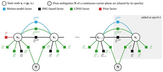
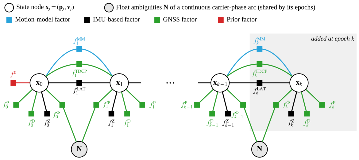
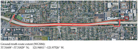
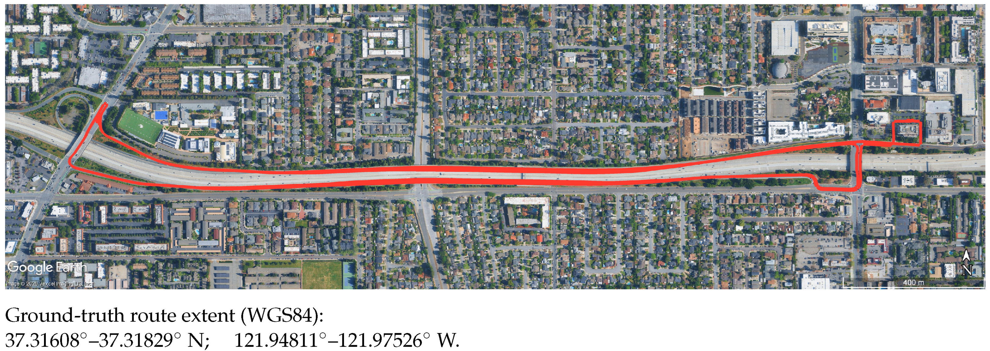
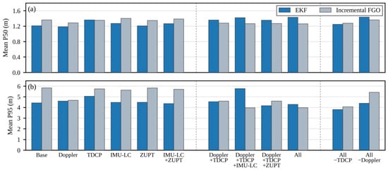
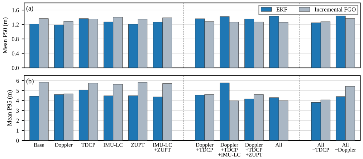
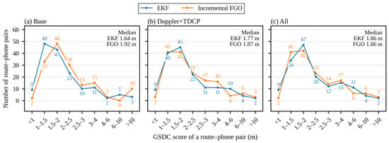
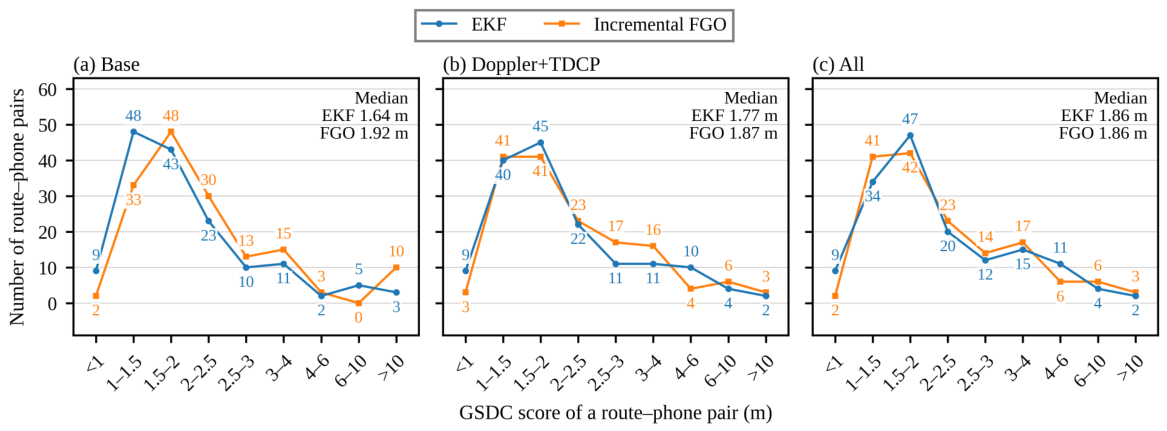
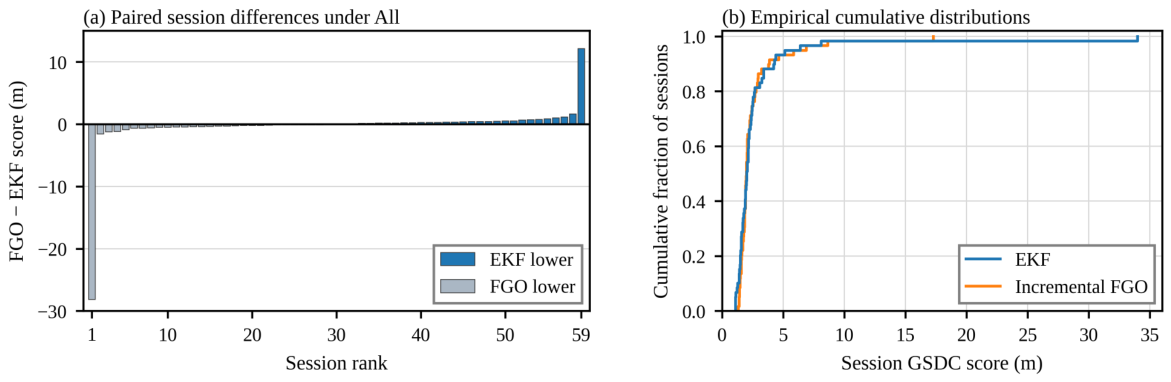
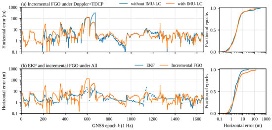
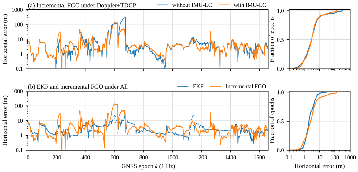
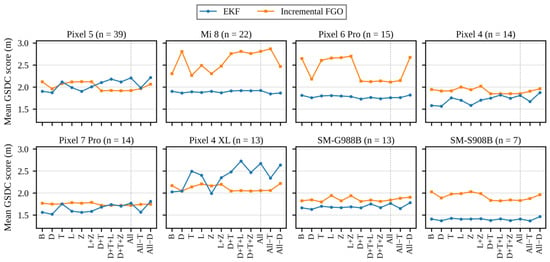
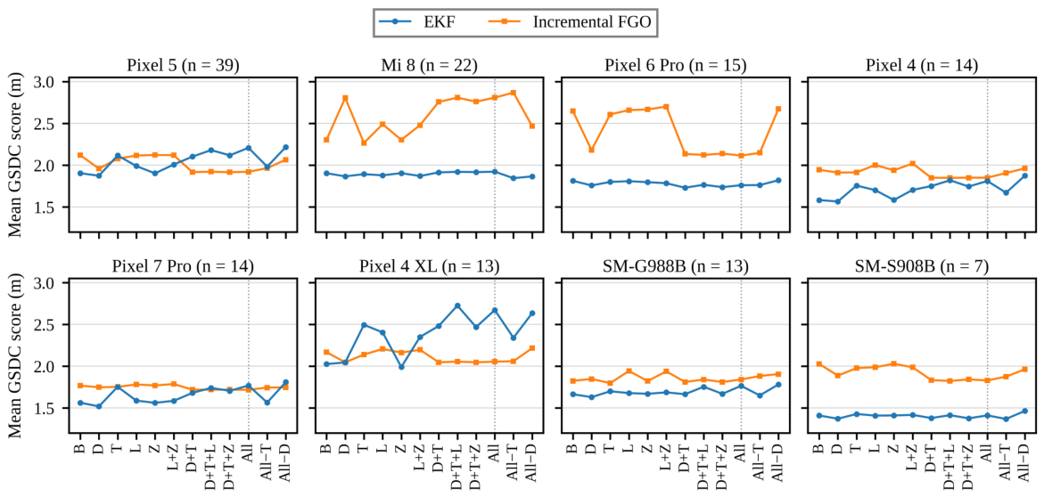
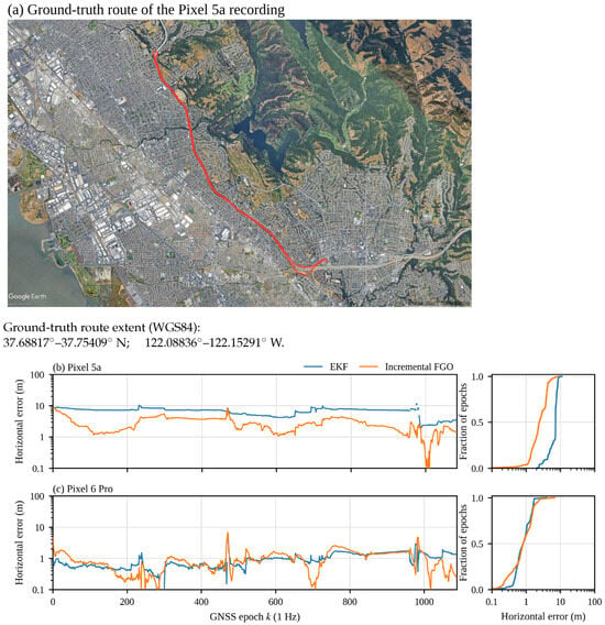
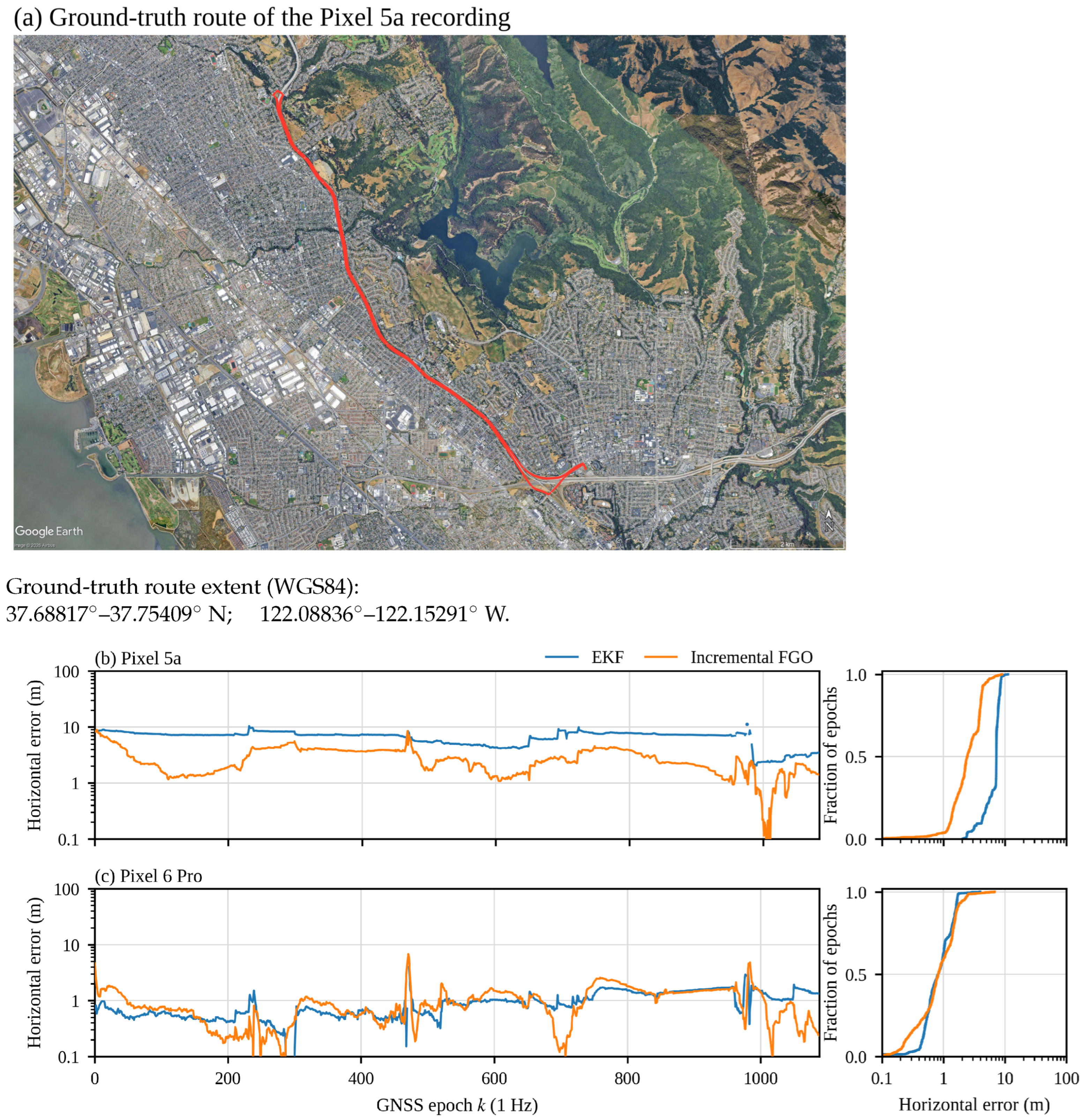
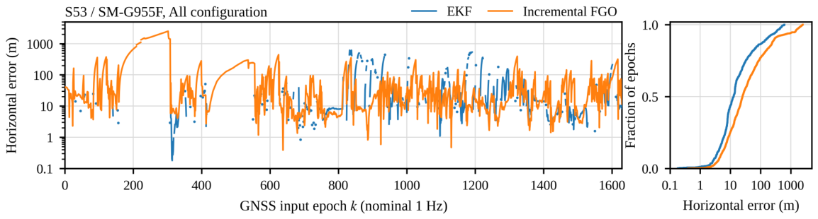

Disclaimer/Publisher’s Note: The statements, opinions and data contained in all publications are solely those of the individual author(s) and contributor(s) and not of MDPI and/or the editor(s). MDPI and/or the editor(s) disclaim responsibility for any injury to people or property resulting from any ideas, methods, instructions or products referred to in the content. |
© 2026 by the authors. Licensee MDPI, Basel, Switzerland. This article is an open access article distributed under the terms and conditions of the Creative Commons Attribution (CC BY) license.