


Abstract
Accurate sulfur dioxide (SO2) estimation is important for sulfur recovery unit (SRU) monitoring when reliable one-step information is required between analyzer observations. This study proposes the Gated Residual Autoregressive–Exogenous GRU Network (GRAG-Net), which separates multivariate process dynamics from strictly causal SO2 history, predicts branch-specific residual corrections relative to the latest measured target, and combines them through a sample-dependent gate. The model was evaluated on 10,081 chronologically ordered industrial observations using three expanding future test periods and five final random seeds. Comparators included persistence, linear extrapolation, absolute and residual classical regressors, process-only and autoregressive GRUs, a joint GRU, LSTM–ARX, TCN–ARX, fixed fusion, and global gating. Across 15 descriptive fold–seed evaluations, GRAG-Net achieved MAE mole%, RMSE mole%, and . Pooled seed-ensemble MAE and RMSE were and mole%, reductions of and relative to AR–GRU. Independently trained ablations identified residual reconstruction and sample-dependent fusion as the main architectural contributors, while dependence-aware bootstrap analysis, causal gate diagnostics, lag analysis, and cross-fold/cross-seed SHAP stability supported robust and interpretable one-step soft sensing.
1. Introduction
Sulfur dioxide (SO2) is an important atmospheric pollutant associated with industrial combustion, mineral processing, petroleum refining, and other sulfur-intensive operations. Following emission, SO2 participates in atmospheric oxidation and aerosol-formation processes that contribute to acid deposition, visibility degradation, and fine-particle formation [1]. Exposure to polluted air is also associated with a substantial global burden of respiratory and cardiovascular disease [2]. In petroleum refineries, accurate monitoring of sulfur compounds is therefore required not only for environmental compliance, but also for maintaining stable process operation, detecting abnormal conditions, and supporting timely corrective action.
Sulfur recovery units (SRUs) convert hydrogen-sulfide-rich acid gases into elemental sulfur, commonly through a thermal stage followed by catalytic Claus conversion and downstream tail-gas treatment. The residual H2S and SO2 concentrations depend on interacting feed conditions, airflow distribution, reaction conditions, catalyst state, and process inertia [3,4]. These relationships are nonlinear and time-dependent, and the effects of an operating adjustment may not be observed immediately because of transport delays and internal process dynamics. Hardware analyzers provide the reference gas-concentration measurements, but their readings can be delayed and their operation requires calibration and maintenance. Data-driven soft sensors can therefore provide complementary real-time estimates for monitoring and diagnostic support [3,5]. In the deployment setting considered here, the hardware analyzer remains the reference measurement source: GRAG-Net estimates the current SO2 concentration from process measurements available through time t and measured analyzer history available only through . The soft sensor is therefore intended to complement the analyzer by providing a model-based one-step estimate between successive validated measurements or during measurement delay; it is not intended to permanently replace the physical analyzer. Continued analyzer measurements remain necessary for reference supervision, performance monitoring, and provision of the causal autoregressive history. Sustained analyzer-outage forecasting, in which predictions must recursively replace missing analyzer values, is outside the scope of this study.
A soft sensor estimates a difficult, delayed, or costly quality variable from routinely measured process information. Data-driven soft sensors are particularly attractive when sufficiently accurate first-principles models are unavailable or too expensive for online use [6,7,8]. Their practical development, however, is complicated by correlated measurements, nonlinear behavior, temporal dependence, measurement imperfections, limited target observations, and changes in operating conditions. Model reliability can deteriorate under process drift, catalyst aging, equipment fouling, raw-material variation, and transitions between operating regimes [9,10]. These characteristics make both dynamic representation and leakage-aware temporal validation essential for industrial soft sensing.
Research on the benchmark SRU process reflects the broader evolution of the field. Early studies considered neural soft analyzers and linear or nonlinear autoregressive models with exogenous inputs [3,11]. Bidar et al. introduced a multi-state-dependent parameter formulation to represent changes in operating state [12], whereas Yuan et al. developed a stacked isomorphic autoencoder for nonlinear feature extraction [13]. Dynamic sequence modeling was later investigated using echo-state networks and recurrent neural networks [14,15]. More recent work has addressed transferability and adaptation through transfer–incremental learning [16], as well as limited labeled data and nonlinear target decomposition through an ISSA–VMD–ESN framework [17]. Collectively, these studies demonstrate the importance of temporal modeling, nonlinear representation, and adaptation in SRU soft sensing.
Dedicated SO2 modeling has also progressed toward increasingly complex temporal architectures. Thameem et al. compared conventional machine learning methods, multilayer perceptrons, one-dimensional convolutional networks, LSTMs, and a CNN–LSTM encoder–decoder for multi-horizon SO2 forecasting in an industrial SRU [4]. Sun et al. subsequently proposed a multistage framework combining variational mode decomposition, CEEMDAN, entropy-guided component reconstruction, an enhanced PatchTST model, and metaheuristic hyperparameter optimization for SRU sulfur gas forecasting [18]. Li and Hao developed a dual-path dynamic soft sensor in which a TCN–Transformer processes auxiliary process variables and a GRU processes historical target values; the two learned representations are combined by summation before final prediction [19]. These recent studies confirm that process-variable histories and target histories provide complementary information. They also expose a remaining question: how should their relative contributions be adjusted when the local operating condition changes?
Existing SRU models generally improve the overall representation through deeper encoders, decomposition, transfer learning, or fixed feature fusion. However, three limitations remain relevant to the present problem. First, process measurements and historical SO2 values represent physically different predictive mechanisms. The latter primarily describe persistence and process inertia, whereas the former provide evidence of process-induced deviation. Embedding both sources in one representation, or combining them using a fixed operation, does not explicitly preserve this distinction. Second, the reliability of the two sources is sample dependent: target persistence can be highly effective under quasi-steady operation but less responsive during rapid transitions, while exogenous airflow information may become more valuable when the process state changes. Third, average test metrics alone do not reveal whether an adaptive fusion mechanism responds meaningfully to branch disagreement, changing operating conditions, or high-change target regimes. In addition, performance estimation for nonstationary time series should preserve temporal order and should separate model selection from evaluation on future observations [20].
To address these limitations, this study proposes the Gated Residual Autoregressive–Exogenous GRU Network (GRAG-Net) for one-step dynamic SO2 soft sensing. GRAG-Net contains two independently parameterized recurrent branches. The process branch encodes a multivariate history of five routinely measured airflow variables, whereas the autoregressive branch encodes only the strictly causal SO2 history. Rather than predicting the absolute concentration independently, each branch estimates a residual correction relative to the most recent available analyzer value. A context-dependent gate then combines the two corrections according to
where and denote the process-driven and autoregressive residual corrections, respectively. The gate is conditioned on the projected features of both branches, the latest SO2 value, the disagreement between the two proposed corrections, and the most recent change in the process variables. Thus, GRAG-Net performs sample-wise soft routing between process-driven and history-driven information instead of applying a global fusion weight. A robust Huber objective is used to reduce excessive sensitivity to isolated large errors [21].
The main contributions of this study are as follows:
- A dual-branch residual architecture is developed in which exogenous process dynamics and autoregressive SO2 persistence are encoded separately and fused through a sample-dependent reliability gate.
- The estimation task is defined explicitly as causal rolling one-step soft sensing: process measurements are available through time t, measured SO2 history is available only through , and neither the current target nor future targets are supplied to the model. Sustained analyzer-outage forecasting is therefore outside the scope of the present study.
- The comparative evaluation is expanded to include persistence and linear extrapolation, absolute and residual classical ARX regressors, strict process-only and autoregressive GRUs, a joint GRU, LSTM–ARX, TCN–ARX, equal-weight fusion, and a global-gate control, in addition to the proposed dynamic gate.
- Architectural claims are tested using independently trained ablations of the residual formulation, fusion mechanism, branch supervision, gate-balance regularization, disagreement input, and process-change input. Chronological folds are treated as the primary evaluation periods, and paired moving-block bootstrap intervals are used to quantify uncertainty in sample-level error differences.
- The diagnostic analysis is made inference-aware: gate associations are evaluated against causal inputs, process–target delays are estimated using training-only lagged correlations, and SHAP explanations are aggregated across folds and seeds with explicit rank-stability analysis.
The experiments use a chronologically ordered industrial benchmark containing 10,081 observations, five airflow-related process measurements, and SO2 concentration as the target [3,22]. The task is formulated as causal one-step soft sensing: process measurements available at time t are combined with target observations available only through . The current target and all future target values are excluded from the model input.
The remainder of this paper is organized as follows. Section 2 describes the dataset, causal sample construction, nested model development protocol, GRAG-Net architecture, benchmark models, evaluation criteria, and interpretability procedures. Section 3 presents the comparative and diagnostic results. Section 4 summarizes the principal findings, industrial implications, limitations, and future research directions.
2. Materials and Methods
This section describes the industrial sulfur recovery unit (SRU) dataset, the causal formulation of the dynamic soft-sensing task, the proposed Gated Residual Autoregressive–Exogenous GRU Network (GRAG-Net), the reference models, and the nested chronological model development protocol. Particular attention is given to preserving the temporal ordering of the plant records and to maintaining a strict separation between hyperparameter selection and final performance estimation. All preprocessing parameters, model configurations, and epoch-selection decisions were derived exclusively from the training information available within the corresponding chronological fold. The evaluation framework further considers chronological robustness, variability across random initializations, target-change regimes, residual behavior, and model interpretability.
2.1. Industrial Sulfur Recovery Process and Dataset
2.1.1. Process Background and Data Source
The experimental data were obtained from a benchmark industrial sulfur recovery process associated with the fourth tail-gas line of an Italian refinery [3,22]. An SRU converts hydrogen-sulfide-rich acid gas streams into elemental sulfur, typically through a high-temperature thermal stage followed by catalytic Claus conversion and downstream tail-gas treatment. In the studied process, acid gas streams originating from the monoethanolamine (MEA) and sour-water-stripping (SWS) sections are combined with controlled air streams before entering the reaction system. The distribution of combustion and secondary air affects the stoichiometric balance of the sulfur-recovery reactions and, consequently, the residual sulfur-compound concentrations measured in the treated tail gas.
The mapping from routinely measured airflow variables to the resulting SO2 concentration is nonlinear and time dependent. Variations in acid gas loading, air allocation, reaction conditions, catalyst state, and downstream treatment do not necessarily affect the measured tail-gas composition instantaneously. Instead, transport delay, process inertia, nonlinear reaction behavior, and interactions among operating variables can produce delayed and regime-dependent responses. These characteristics make the dataset suitable for evaluating dynamic soft sensors that explicitly retain both recent process history and target persistence.
The observations were recorded at one-minute intervals. The original benchmark contains five process measurements and two sulfur gas outputs, H2S and SO2. The present study focuses exclusively on SO2 soft sensing; therefore, the analyzed data matrix contains the five process inputs and the SO2 target field, denoted by y2. Following column selection and numeric conversion, the retained dataset comprised
complete observations in their original chronological order. No missing values were present in the retained variables, and no interpolation or imputation was therefore required. The five deposited process channels are supplied on a scaled benchmark representation, whereas the SO2 target retains the concentration scale used in the originating SRU data and is reported in mole%. This interpretation is consistent with both the original refinery study and the recent public benchmark release [3,18]. The chronological order was preserved throughout the study, and no random shuffling was applied before constructing the training, validation, and test periods.
2.1.2. Process Variables and Prediction Target
Let
denote the process measurements available at sampling instant t. The corresponding target is the SO2 concentration , reported in mole%.
The five airflow-related channels were treated as exogenous process measurements because they are routinely available from the plant instrumentation, whereas SO2 represents the difficult-to-measure quality variable estimated by the soft sensor. The process channels retain their benchmark scaling, while SO2 is reported in mole%. Physical variable names are retained in all tables, figures, lagged-feature labels, and SHAP explanations to preserve process-level interpretability.
2.1.3. Descriptive and Distributional Characteristics
Table 1 reports descriptive statistics for the complete benchmark dataset. These statistics are provided only to characterize the benchmark; they were not used to preprocess validation or test observations. Fold-specific preprocessing parameters were estimated from the relevant training block, as described in Section 2.2.
Table 1.
Descriptive statistics of the industrial SRU benchmark ( 10,081).
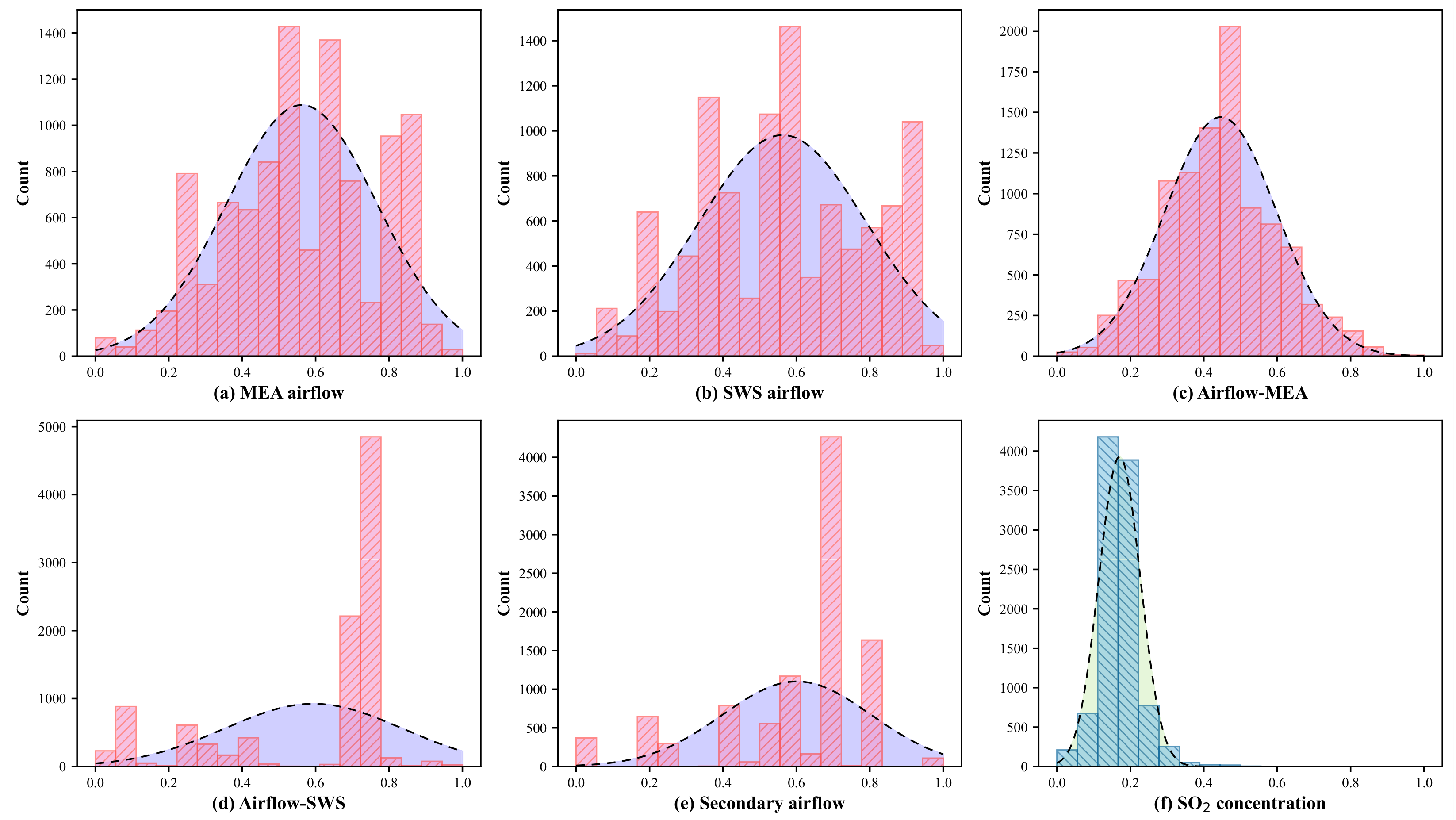
The SO2 concentration is concentrated within a comparatively narrow operating range, with a mean of , a median of , and a standard deviation of . Its third quartile is , despite a maximum of mole%, indicating that large concentration values are relatively infrequent. In contrast, the process measurements span broader and heterogeneous operating ranges. The median values of airflow in the SWS zone () and secondary airflow () are and , respectively, showing that these channels operate near their upper benchmark-scaled regions during a substantial part of the observation period. Airflow in the MEA zone () is more centrally concentrated and exhibits the smallest process-variable standard deviation.
The histogram and density plots in Figure 1 show that several process variables have heterogeneous and visibly multimodal distributions. These modes indicate recurring operating regions rather than one stationary Gaussian regime. The SO2 target has a narrow dominant distribution with a sparse upper tail. This imbalance is relevant because a model may achieve a low average error in the dominant quasi-steady region while remaining less accurate during rare concentration excursions.
Figure 1.
Histogram and density distributions of the five benchmark-scaled SRU process variables and SO2 concentration. The process measurements exhibit heterogeneous and partly multimodal operating distributions, whereas the target is concentrated within a narrow dominant range with a sparse upper tail.
2.1.4. Correlation Structure and Target Persistence
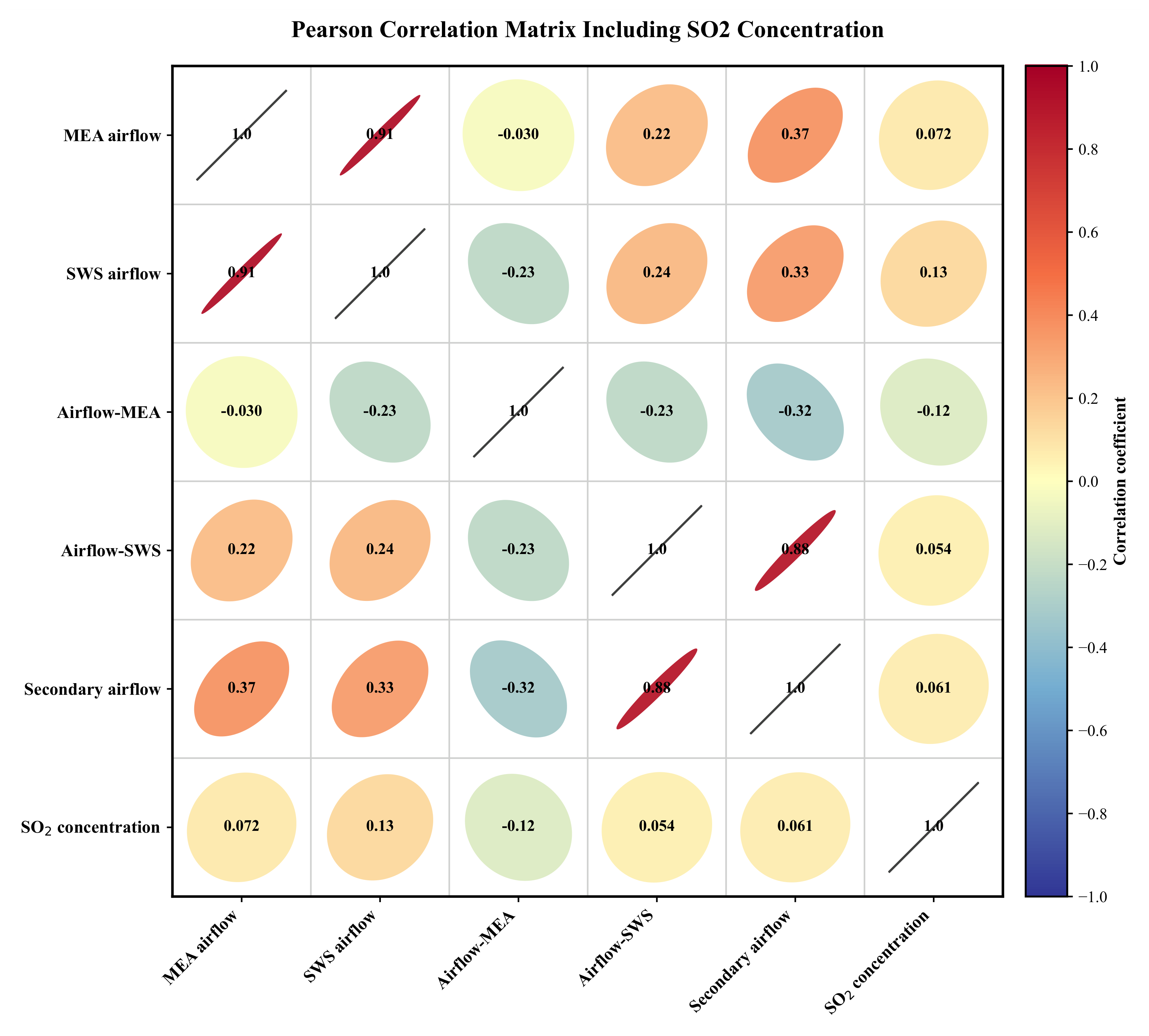
The Pearson correlation structure is shown in Figure 2. Strong dependence is present among selected process variables. The largest positive process-input correlations are observed between MEA airflow and SWS airflow,
and between airflow in the SWS zone and secondary airflow,
These values indicate substantial coupling and partial redundancy among the airflow measurements. In contrast, the zero-lag correlations between the five process variables and SO2 range approximately from to .
The weak instantaneous input–target correlations do not imply that the process measurements are uninformative. Instead, they suggest that their effects on SO2 are delayed, nonlinear, dependent on interactions among variables, or conditional on the operating regime. This observation motivates the use of historical multivariate process windows rather than a static mapping based only on measurements recorded at the current instant.
In contrast to the weak zero-lag process–target associations, the SO2 sequence exhibits pronounced short-term persistence. The autocorrelation coefficients at lags one through five are
The lag-one autocorrelation of confirms that the most recent SO2 observation is a strong local predictor and motivates its use as the persistence reference in GRAG-Net. However, the gradual decay across subsequent lags shows that the useful temporal information is not restricted to a single previous observation. This supports a sequence-based autoregressive encoder with a history length selected through nested hyperparameter optimization.
Figure 2.
Pearson correlation ellipse matrix for the five SRU process variables and SO2 concentration. Ellipse orientation indicates the sign of the relationship, whereas increasing eccentricity denotes stronger linear dependence.
Taken together, the exploratory analysis identifies three properties that directly motivate the proposed methodology: (i) heterogeneous and partly multimodal process-variable distributions; (ii) weak instantaneous but potentially delayed and nonlinear process–target relationships; and (iii) strong short-term target persistence. These characteristics support the separation of process history and target history into two distinct temporal pathways before their contributions are fused dynamically.
2.2. Problem Formulation and Causal Sample Construction
2.2.1. One-Step Dynamic Soft-Sensing Formulation
The objective is to estimate the current SO2 concentration from two information sources that are available at sampling instant t: (i) the recent history of the five routinely measured process variables and (ii) a strictly causal history of previously observed SO2 values. The task is therefore formulated as one-step dynamic soft sensing, rather than unconstrained recursive forecasting. Current process measurements are assumed to be available from the distributed control system at time t, whereas the target history channel terminates at . Consequently, neither the current target nor any future target value is exposed to the model.
Let the instantaneous process vector be
A multivariate process-history window of length is defined as
while the strictly causal SO2 history of length is
The complete information set available for estimating is therefore
The general soft-sensing mapping is expressed as
where denotes a nonlinear estimator with parameters . For GRAG-Net, is extracted from the final element of and is used explicitly as both a gating-context variable and the residual reference in the final reconstruction. The proposed mapping can therefore be written more specifically as
The two histories represent different predictive mechanisms. The process window describes the recent operating trajectory and provides exogenous evidence of process-driven changes, whereas captures target persistence and process inertia. Their history lengths are allowed to differ because the useful temporal extent of the process variables need not match that of the target. Both and are therefore selected independently within the nested hyperparameter-optimization procedure.
2.2.2. Fold-Specific Standardization
Although the process channels are supplied on a scaled benchmark representation and SO2 is retained in mole%, an additional z-score transformation was applied to improve numerical conditioning and to ensure that each model was developed using only the distributional information available in its training period. For process variable ,
and the target was transformed as
Here, , , , and were estimated exclusively from the training block available at the corresponding stage of the nested protocol. During inner hyperparameter optimization, the transformations were fitted only to the inner-training subset and were then applied unchanged to the inner-validation subset. After hyperparameter selection, new transformations were fitted to the complete outer-training block and applied unchanged to its held-out outer-test block.
The standardized history tensors are denoted by and . Neural-model training and prediction were performed in the standardized target domain. Each estimate was subsequently returned to the original benchmark scale using
before computing the reported evaluation metrics.
2.2.3. Sliding-Window Sample Generation
Dynamic samples were constructed with a stride of one observation. Under the zero-based indexing used in the implementation, the first admissible target index for a given pair is
which guarantees that both the complete process window in Equation (8) and the complete target history sequence in Equation (9) are available. For each admissible t, one supervised sample was formed as
No downsampling, interpolation, or random reordering was applied during window construction.
The history lengths were treated as model hyperparameters rather than fixed a priori. The searched values were
Because the records were sampled at one-minute intervals, these values correspond to process histories of 16, 32, or 64 min and target histories of 4, 8, 16, or 32 min.
2.2.4. Causality and Chronological Boundary Handling
The chronological split boundaries were defined in terms of prediction indices, not isolated window matrices. At the beginning of a validation or test block, observations immediately preceding the boundary were retained as historical context when they belonged to the information set . This treatment reflects online deployment: when the first sample of a future period is estimated, the recent process measurements and the valid analyzer observations recorded before that instant are already available.
For every prediction index t, the process sequence terminates at and the target sequence terminates at . Thus, historical context may cross a training–validation or training–test boundary, but the prediction target itself and all future values remain excluded. The procedure does not create a gap between adjacent chronological blocks and does not discard the first or observations of each held-out period unnecessarily.
During outer-test evaluation, each prediction uses the measured SO2 history available through . Predictions are not recursively fed back as substitutes for subsequent analyzer measurements. The reported task therefore represents a rolling one-step inferential setting in which a recent valid target history is available for every sample. This assumption should be distinguished from prolonged analyzer-outage forecasting, which would require recursive prediction and is outside the scope of the present study.
2.2.5. Input Representation for the Baseline Models
The classical autoregressive–exogenous baselines cannot directly process two-dimensional sequences. Their standardized process and target histories were therefore flattened and concatenated:
The same causal information was consequently supplied to all learnable models, while only its representation differed. The support vector regressor and tree ensembles received , whereas GRAG-Net retained the temporal organization of and and processed the two histories through independent recurrent branches. This design ensures that comparative performance differences are not caused by unequal access to process or target history information.
2.3. Proposed GRAG-Net Architecture
2.3.1. Design Rationale and Architectural Overview
The proposed Gated Residual Autoregressive–Exogenous GRU Network (GRAG-Net) is designed to model two complementary mechanisms governing one-step SO2 soft sensing. The first mechanism is the strong short-term persistence of the target, which makes the most recent valid SO2 observation an informative reference under quasi-steady operation. The second mechanism is the process-driven deviation from this recent trajectory, which is reflected in the evolving histories of the five airflow-related variables. Because the relative usefulness of these two information sources can change from one observation to another, GRAG-Net models them through independent temporal branches and combines their residual corrections using a sample-dependent reliability gate.
Let and denote the standardized process and target history windows defined in Section 2.2. Rather than predicting the absolute target independently, each branch estimates a correction relative to the latest standardized SO2 observation . The complete model is summarized by
Here, and denote the process and autoregressive experts, respectively, while denotes the gating network. A value of approaching one gives greater influence to the process-driven correction, whereas a value approaching zero favors the autoregressive correction.
This residual formulation is particularly suitable for the studied target. The skip connection through explicitly preserves the strong persistence component, allowing the trainable branches to focus on the remaining change:
Thus, GRAG-Net does not force either branch to repeatedly learn the near- identity mapping between consecutive target observations. Instead, both branches solve the more focused problem of estimating how the current target departs from its latest measured value.
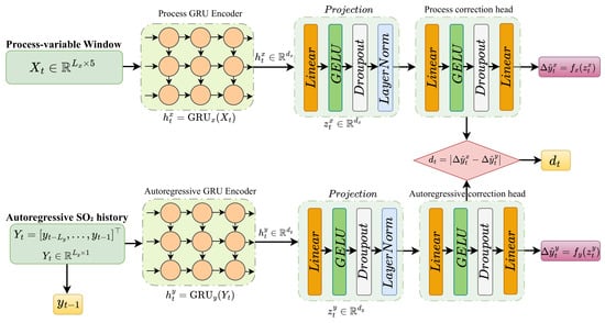
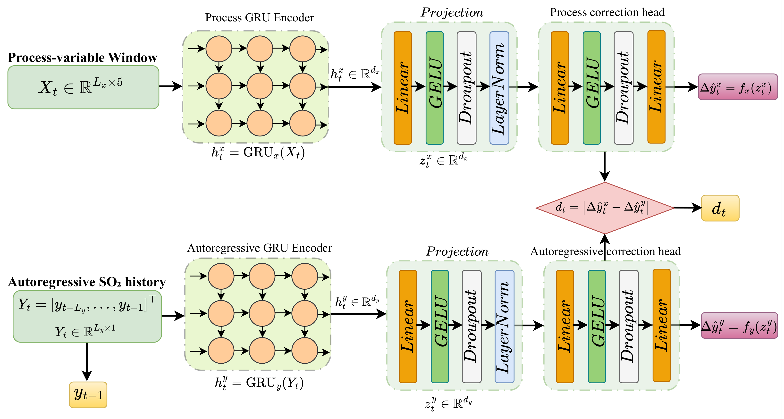
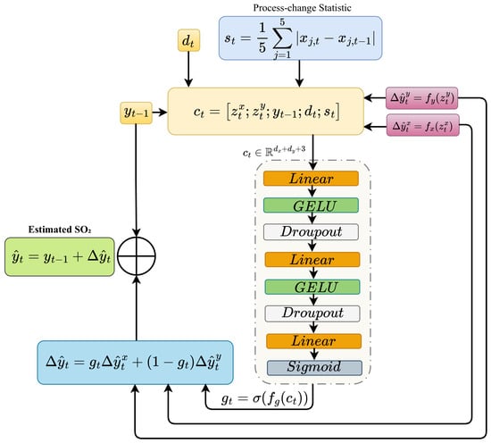
Figure 3 and Figure 4 present the architecture in two complementary parts. Figure 3 illustrates the independent temporal encoders, projection modules, and branch-specific correction heads, while Figure 4 shows the dynamic context, reliability-gate estimation, residual fusion, and final reconstruction. Sequence dimensions are denoted symbolically by and .
Figure 3.
Dual-branch temporal encoding and residual-correction module of GRAG-Net. The process branch encodes the multivariate operating history, whereas the autoregressive branch encodes the strictly causal SO2 history. Each branch produces a dedicated residual correction relative to , and the absolute difference between the two corrections defines the branch-disagreement statistic .
Figure 4.
Context-dependent reliability gating and residual fusion in GRAG-Net. The projected process and autoregressive states, latest SO2 observation, branch disagreement, and recent process-change statistic form the gating context. The resulting process weight adaptively combines the two branch-specific residual corrections before addition to the persistence reference.
2.3.2. GRU-Based Temporal Encoding
A gated recurrent unit (GRU) was selected for both temporal branches because it provides explicit memory-control mechanisms with fewer trainable gates than an LSTM. For an input vector and previous hidden state , a GRU computes
where and are the reset and update gates, denotes the logistic sigmoid, and ⊙ represents element-wise multiplication. Separate parameter sets are learned for the process and autoregressive GRUs; no recurrent weights are shared between the two branches.
2.3.3. Process-Variable Expert
The process expert receives the standardized sequence and models nonlinear temporal interactions among the five process measurements. Its final GRU state is
where is the process-branch hidden dimension. The final state is passed through a projection block consisting of a linear transformation, Gaussian error linear unit (GELU), dropout, and layer normalization:
Layer normalization stabilizes the latent scale before fusion, whereas dropout regularizes the projected representation.
A two-layer correction head maps to a scalar process-driven residual:
The implemented head follows
The resulting branch-level estimate is
Accordingly, the process expert learns the correction implied by the recent evolution of the airflow-related measurements.
2.3.4. Autoregressive Expert
The autoregressive expert independently encodes the strictly causal target history. Its final hidden state is
where is selected independently from . The projected autoregressive representation is
Its correction head is defined as
with layer sequence
The corresponding branch-level estimate is
This branch provides a history-driven correction that exploits the shape, direction, and persistence of the recent SO2 trajectory rather than using only the single value .
2.3.5. Dynamic Context Construction
The reliability gate receives the learned representations of both experts together with two explicit dynamic descriptors. The first descriptor is the absolute disagreement between the proposed branch corrections:
A small value of indicates that the two experts recommend a similar departure from the persistence reference, whereas a large value indicates competition between their process-driven and history-driven explanations.
The second descriptor summarizes the most recent change in the standardized process measurements:
This statistic supplies the gate with a compact indicator of the local process dynamics. It is not used as a manually defined regime label and does not directly determine the gate value; instead, it is learned jointly with the latent branch representations.
The complete context vector is
Including allows the gating decision to depend on the current target level, while and expose the instantaneous degree of branch disagreement and process variation.
2.3.6. Sample-Dependent Reliability Gate and Residual Fusion
The context vector is mapped to a scalar process-branch weight using a three-layer multilayer perceptron:
The implemented sequence is therefore
The gate performs soft routing rather than hard branch selection. The fused residual is
and the final standardized estimate is reconstructed as
Because is computed independently for each sample, the relative branch contribution can vary throughout the operating sequence. The prediction on the original benchmark scale is obtained using the inverse transformation in Equation (15).
2.3.7. Joint Training Objective
A robust Huber loss is used because the target distribution contains a narrow central region together with infrequent large deviations. For a scalar residual e and transition parameter , the loss is
The transition value was fixed at in the standardized target domain. For a mini-batch of size B, the principal prediction loss is
Optimizing only the fused output can permit one expert to become weak while the gate collapses toward the other. To preserve two individually predictive experts, the branch-level estimates in Equations (34) and (40) are supervised through
This auxiliary objective encourages both branches to remain informative before fusion; it does not force their residual corrections to be identical.
A weak gate-balance term can additionally discourage premature batch-level collapse toward a single branch:
The regularizer constrains only the average gate value within a mini-batch and does not require every sample to receive equal process and autoregressive weights. The complete objective is
where and are selected within the inner hyperparameter-optimization loop. When , routing is governed entirely by the predictive and branch-supervision objectives.
2.3.8. Training-Time Autoregressive Perturbation
To reduce excessive dependence on a perfectly noise-free target history, zero-mean Gaussian perturbation is considered as a training-only regularizer:
When perturbation is active, the residual reference provided to the model is the final perturbed history value,
so that the autoregressive sequence and skip connection remain internally consistent. The process history and regression target remain unperturbed. No noise is applied during validation or outer-test evaluation. The standard deviation is selected through the inner optimization procedure.
2.3.9. Architecture Summary
Table 2 summarizes the implemented modules and tensor dimensions. GRAG-Net remains compact because each information source is processed by one recurrent layer and the fusion mechanism consists of a small multilayer perceptron.
Table 2.
Implemented GRAG-Net modules, layer configurations, and output dimensions.
2.4. Comparator Models and Formal Ablations
The revised evaluation was designed to separate three questions: whether target persistence alone is sufficient, whether conventional or sequence-based models can exploit the same causal information, and whether the proposed residual dual-branch gate provides value beyond simpler fusion rules. All learnable models were fitted using only information available within the corresponding outer-training period.
Two parameter-free references were included. Persistence uses , while linear extrapolation extends the most recent target increment, . Four classical regressors—SVR [23], Random Forest [24], Extra Trees [25], and XGBoost [26]—were evaluated in both absolute-target ARX form and residual form. The residual variants predict and reconstruct the target by adding the predicted increment to ; this control is important because it separates the effect of residual learning from the recurrent architecture.
The sequence-model controls comprised a strict process-only GRU, an AR–GRU using only causal target history, a joint GRU receiving combined process and target history information, LSTM–ARX, and TCN–ARX. The process-only GRU receives neither target history samples nor the residual anchor. Two fusion controls use the same dual-branch information as GRAG-Net: equal fusion fixes the branch weight at , whereas the global-gate model learns one scalar fusion weight shared by all samples. These controls distinguish the value of sample-dependent routing from the mere availability of two branches.
Formal ablations were independently trained for the full GRAG-Net, removal of the residual reconstruction, equal fusion, global gating, removal of branch supervision (), removal of gate-balance regularization (), removal of branch disagreement , and removal of the process-change statistic . AR-history perturbation is not interpreted as an active component of the selected final model because hyperparameter selection returned in all three outer folds.
2.5. Chronological Model Development and Reproducibility
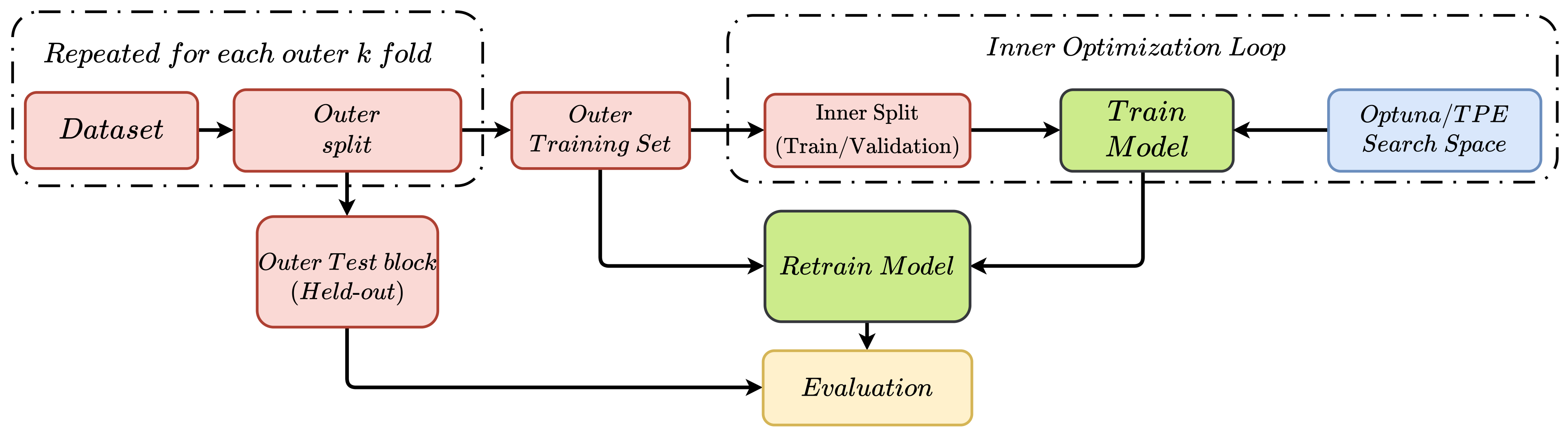
2.5.1. Nested Chronological Design
Random partitioning was avoided because neighboring SRU samples are strongly autocorrelated and time-ordered evaluation is required to avoid optimistic performance estimates in autoregressive settings [27]. Three expanding outer-training periods were therefore followed by non-overlapping future evaluation periods, as summarized in Table 3. The outer-test targets were excluded from model fitting, preprocessing, hyperparameter selection, and epoch selection. During test-time rolling one-step evaluation, however, an SO2 observation becomes admissible historical information after its time has passed; thus a prediction at t may use measured target history only through . Predicted targets are never recursively fed back.
Table 3.
Chronological outer folds used for final evaluation. Intervals are half-open index ranges.
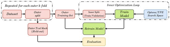
Figure 5 summarizes the nested workflow. Within each outer-training period, the earliest of observations formed the inner-training subset and the latest formed the inner-validation subset. Scaling parameters were estimated only from the active training subset. Optuna [28] with a seeded tree-structured Parzen estimator (2026) was used for configuration selection. Final neural models were evaluated with seeds after all model-selection decisions had been fixed.
Figure 5.
Leakage-aware nested chronological model development. Hyperparameters, preprocessing parameters, and epoch-selection decisions are determined using only the outer-training period. The subsequent future block is held out from model development and is evaluated under causal rolling one-step inference, where measured SO2 history is available only through the preceding time instant.
2.5.2. Hyperparameter Search Spaces and Selected Configuration
To make the revised comparison reproducible, the search domains used for the reviewer-requested models are reported explicitly in Table 4. Search was performed independently inside each outer-training period using the chronological inner split described above; the outer-test block was never used to choose a configuration. Classical models used 18 Optuna trials per fold and neural models used 24 trials per fold. The final reviewer run reused the winning configurations saved from this model development stage, without test-set retuning.
Table 4.
Hyperparameter search spaces used in the nested model development stage. Parameters not listed were fixed by the implementation. Structural ablations used the same numerical search domain while forcing the ablated component to its prescribed setting.
The full GRAG-Net configuration selected independently in each outer fold was identical across all three folds, as summarized in Table 5. This agreement emerged from independent inner-fold selection; the configuration was not imposed globally. In particular, was selected in every fold, so autoregressive history perturbation is not treated as an active component of the final model. Exact fold-specific winning configurations for every comparator and formal ablation, together with the corresponding Optuna trial histories, were retained in the reproducibility outputs. These records are available with the revision materials and permit reconstruction of every reported model-selection decision.
Table 5.
GRAG-Net configuration selected independently in all three chronological outer folds.
After hyperparameter selection, the final training length for each neural model, outer fold, and seed was determined without using the outer-test block. Specifically, the earliest 85% of the corresponding outer-training period was used for fitting and the latest 15% for epoch selection, with a maximum of 150 epochs and early-stopping patience of 15. The selected epoch was then used to retrain the model from a new initialization on the complete outer-training period before evaluation. Thus, the temporary epoch-selection subset was returned to the final training set and no test observation was used to determine training duration.
The final revision was executed under Windows 11 using Python 3.13.9, NumPy 2.3.5, pandas 2.3.3, PyTorch 2.11.0 with CUDA 12.6, scikit-learn 1.7.2, XGBoost 3.2.0, and SHAP 0.51.0 on an NVIDIA T1000 8 GB GPU. The exact chronological splits, selected configurations, fitted preprocessing parameters, epoch-selection histories, model checkpoints, fold–seed predictions, metrics, and diagnostic outputs were retained as a reproducibility audit trail.
2.6. Evaluation, Statistical Analysis, and Diagnostics
All predictions were inverse transformed before evaluation, and SO2 errors are reported in mole%. The primary predictive measures are MAE, RMSE, and ; sMAPE, median absolute error, explained variance, mean bias deviation, and Pearson correlation are retained as secondary diagnostics. Because the five random seeds within one chronological fold share the same test period, the three outer folds are treated as the primary independent evaluation periods; seed dispersion describes optimization variability rather than five additional independent datasets.
For fold k, the main error measures are
The pooled seed-ensemble analysis averages the five predictions for each unique out-of-fold sample before computing metrics over the 4537 non-overlapping test observations. It is reported as a complementary aggregate, not as a replacement for fold-wise evidence.
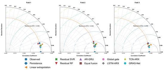
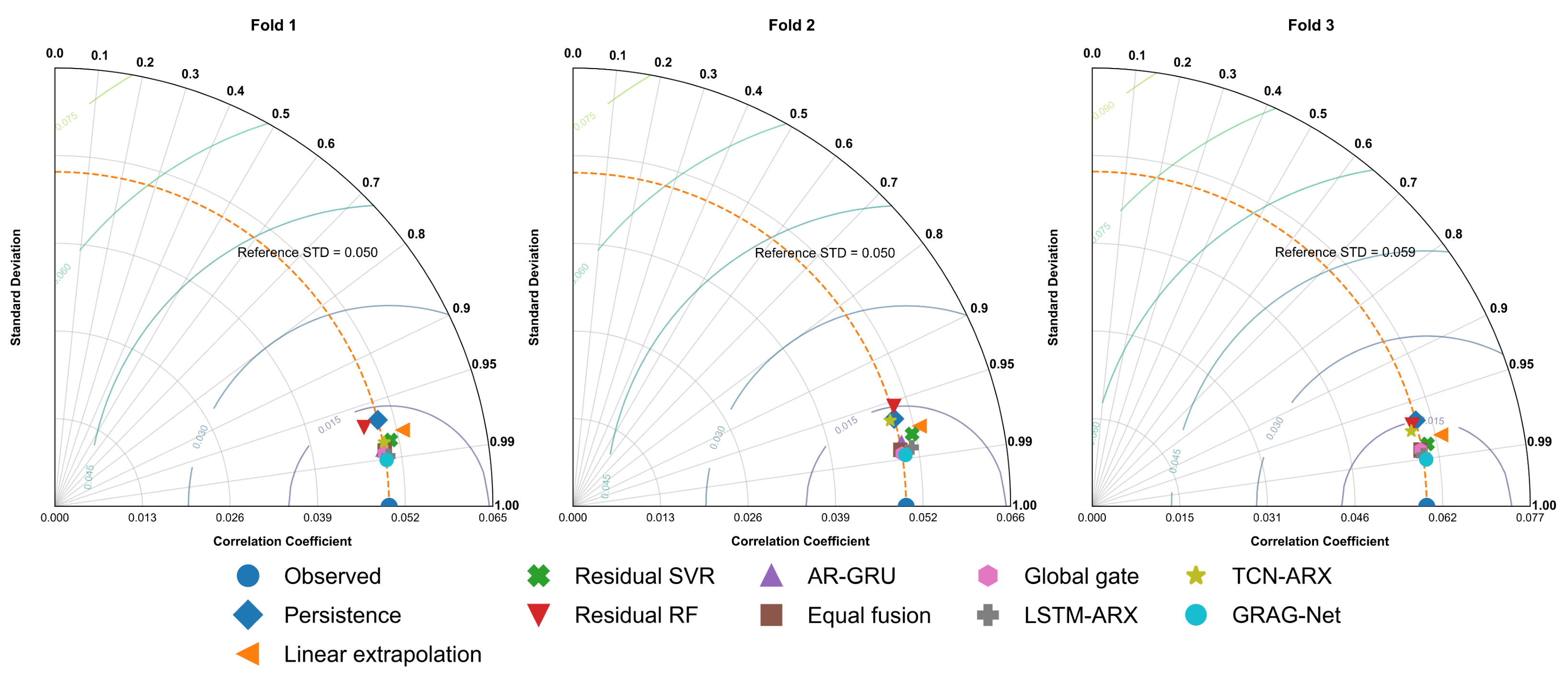
Taylor diagrams are reported separately for the three outer folds. Each model is located by its Pearson correlation and predicted standard deviation, while centered RMSE contours summarize joint discrepancies in phase and variability. The ideal point has correlation one, predicted standard deviation equal to the observed standard deviation, and zero centered RMSE [29].
To quantify uncertainty while respecting serial dependence, paired moving-block bootstrap analysis was applied to sample-wise loss differences
using absolute and squared error losses. A block length of 30 samples is the primary analysis, with 15 and 60 samples retained as sensitivity checks. Negative favors GRAG-Net. Confidence intervals are computed within each chronological test period rather than pooling folds as if they were exchangeable independent replicates.
The diagnostic analysis was deliberately separated into inference-available and retrospective quantities. Gate behavior was summarized by Spearman association between the process-branch weight and three quantities available at inference: branch disagreement , process change , and the latest measured target . Any association with realized branch advantage is treated only as retrospective interpretation because it depends on .
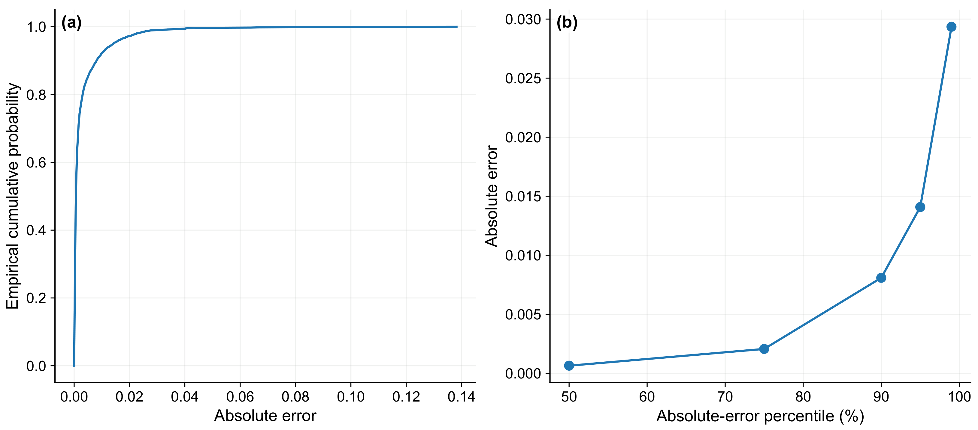
Temporal alignment was examined using training-only lagged Pearson cross-correlations between each process variable and SO2. For each fold, the reported lag is the training-period lag that maximizes ; these correlations are descriptive and are not interpreted as causal delay estimates. Error reliability was assessed using the empirical CDF and the 50th, 75th, 90th, 95th, and 99th percentiles of absolute error. A retrospective target-change analysis partitions test samples by : the lower 50% form the stable regime, the 50th–90th percentiles form the changing regime, and the upper 10% form the large-change regime. This analysis tests whether conclusions depend primarily on quasi-steady observations.
SHAP was computed for two predefined seeds (42 and 52) in each of the three folds. Global importance is based on mean absolute SHAP value aggregated across these six fitted artifacts. Explanation stability is quantified by pairwise Spearman correlation of feature ranks and top-20 Jaccard overlap. SHAP values describe the fitted model and should not be interpreted as causal process effects [30,31].
The public benchmark and the originating SRU literature report SO2 concentration in mole%. The released benchmark does not document the make, calibration uncertainty, accuracy specification, or regulatory tolerance of the plant analyzer used to obtain the reference SO2 measurements. Because these instrument-specific quantities cannot be recovered reliably from the available data, they are not inferred or approximated here. Accordingly, the study reports prediction errors in the available physical concentration unit but does not compare them with an unspecified analyzer-accuracy or compliance threshold.
3. Results and Discussion
The revised experiments assess GRAG-Net under the causal rolling one-step setting defined in Section 2.2. The three non-overlapping chronological test periods are treated as the primary evaluation periods. Five final seeds quantify optimization variability within each fold, while pooled seed-ensemble predictions are reported only as a complementary sample-level summary over the 4537 unique out-of-fold observations.
3.1. Comparative Predictive Performance
Table 6 reports descriptive mean ± standard deviation over the 15 fold–seed evaluations for each model. These values summarize both chronological and initialization variability; they are not interpreted as 15 independent datasets because the five seeds within a fold share the same test observations. GRAG-Net achieved the strongest primary performance, with MAE mole%, RMSE mole%, and . It also obtained the highest Pearson correlation () and the lowest sMAPE () among the learned full-model comparators.
Table 6.
Predictive performance across the three chronological outer folds and five final seeds. Values are descriptive mean ± standard deviation over 15 fold–seed evaluations per model. The three chronological folds, not the 15 repeated runs, are the primary independent evaluation periods; formal paired uncertainty is assessed separately by moving-block bootstrap. The best value is shown in bold and the second-best value is underlined. For MBD, ranking is based on absolute magnitude.
The strongest sequence comparator was LSTM–ARX in RMSE and , whereas linear extrapolation produced the second-lowest MAE. Nevertheless, neither matched GRAG-Net simultaneously in absolute error, squared-error sensitivity, variance explanation, and correlation. The dedicated AR–GRU was also substantially weaker, with MAE and RMSE mole%. Thus, the gain of GRAG-Net cannot be attributed merely to access to recent target history; the exogenous branch and adaptive residual fusion provide additional predictive information beyond a strong autoregressive recurrent model.
MSE and explained variance were also computed and retained in the reproducibility outputs; they are omitted from the main table because they are largely redundant with RMSE and . The residual classical controls additionally show that residualization alone is insufficient: residual SVR is the strongest classical residual model, but its MAE and RMSE remain above those of GRAG-Net. Likewise, equal fusion and global gating improve substantially over the strict process-only model but remain behind the dynamic gate, supporting the value of sample-dependent fusion rather than simply adding a second branch.
The pooled seed-ensemble analysis leads to the same conclusion. GRAG-Net attained MAE mole%, RMSE mole%, and . Relative to persistence, these correspond to MAE and RMSE reductions of and ; relative to AR–GRU, the reductions are and . Because pooling averages the five predictions for each unique sample, these values are complementary ensemble statistics and are not substituted for the fold-level evidence below.
3.2. Chronological Robustness and Temporal Tracking
Table 7 reports fold-wise mean performance over the five final seeds for the principal sequence and fusion models. GRAG-Net has the lowest MAE and RMSE in all three chronological periods. Its MAE ranges from to mole%, while remains between and . The third fold is the most difficult in absolute-error terms, yet the proposed model preserves high explained variance and maintains a clear margin over AR–GRU, LSTM–ARX, TCN–ARX, equal fusion, and global gating.
Table 7.
Fold-level mean performance over five final seeds for the principal sequence and fusion models. Errors are in mole%.
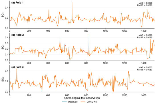
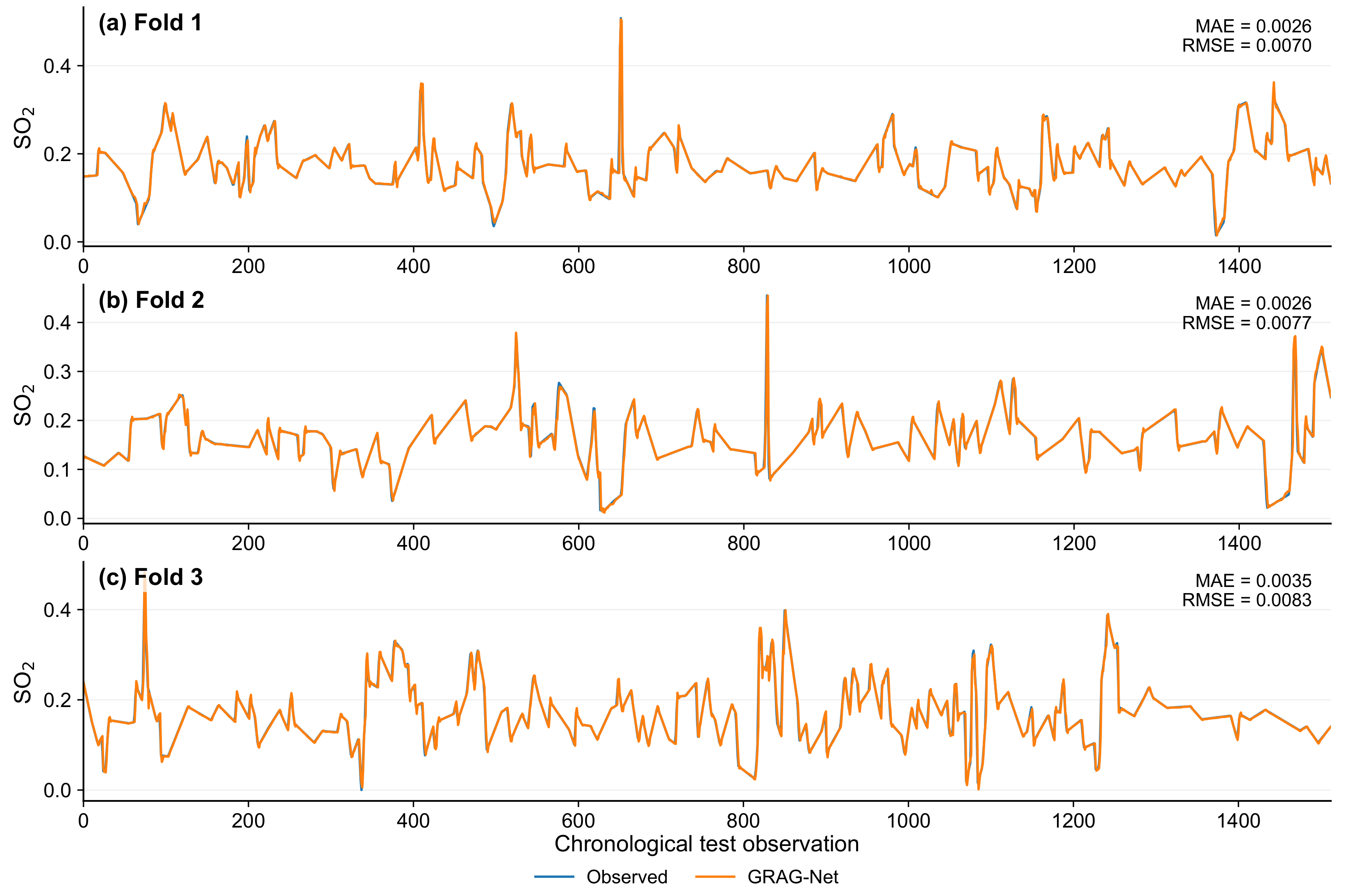
Figure 6 shows the seed-ensemble GRAG-Net trajectories. The ensemble MAE values are , , and mole% for Folds 1–3, respectively, with corresponding RMSE values of approximately , , and mole%. The predicted trajectories closely follow the observed concentration through both steady and rapidly varying intervals, with the largest deviations concentrated around abrupt excursions.
Figure 6.
Observed and GRAG-Net-predicted SO2 concentration over the three chronological outer-test periods. Predictions are seed-ensemble means; fold-specific MAE and RMSE are reported in each panel.
3.3. Taylor-Diagram Assessment
The fold-specific Taylor diagrams in Figure 7 provide a joint view of correlation, variance reproduction, and centered error. GRAG-Net attains correlations of , , and in Folds 1–3 and the lowest centered RMSE in every fold: , , and mole%, respectively. Its predicted standard deviations (, , and ) closely match the corresponding observed values (, , and ). These results indicate that the proposed model not only reduces pointwise error but also reproduces the amplitude and temporal variability of the observed SO2 sequence more faithfully than the evaluated alternatives.
Figure 7.
Taylor diagrams for the three chronological test folds. Radial distance denotes predicted standard deviation, angular position denotes Pearson correlation, and contours denote centered RMSE. The observation is the reference point.
3.4. Formal Ablation of the Proposed Architecture
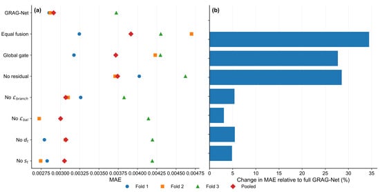
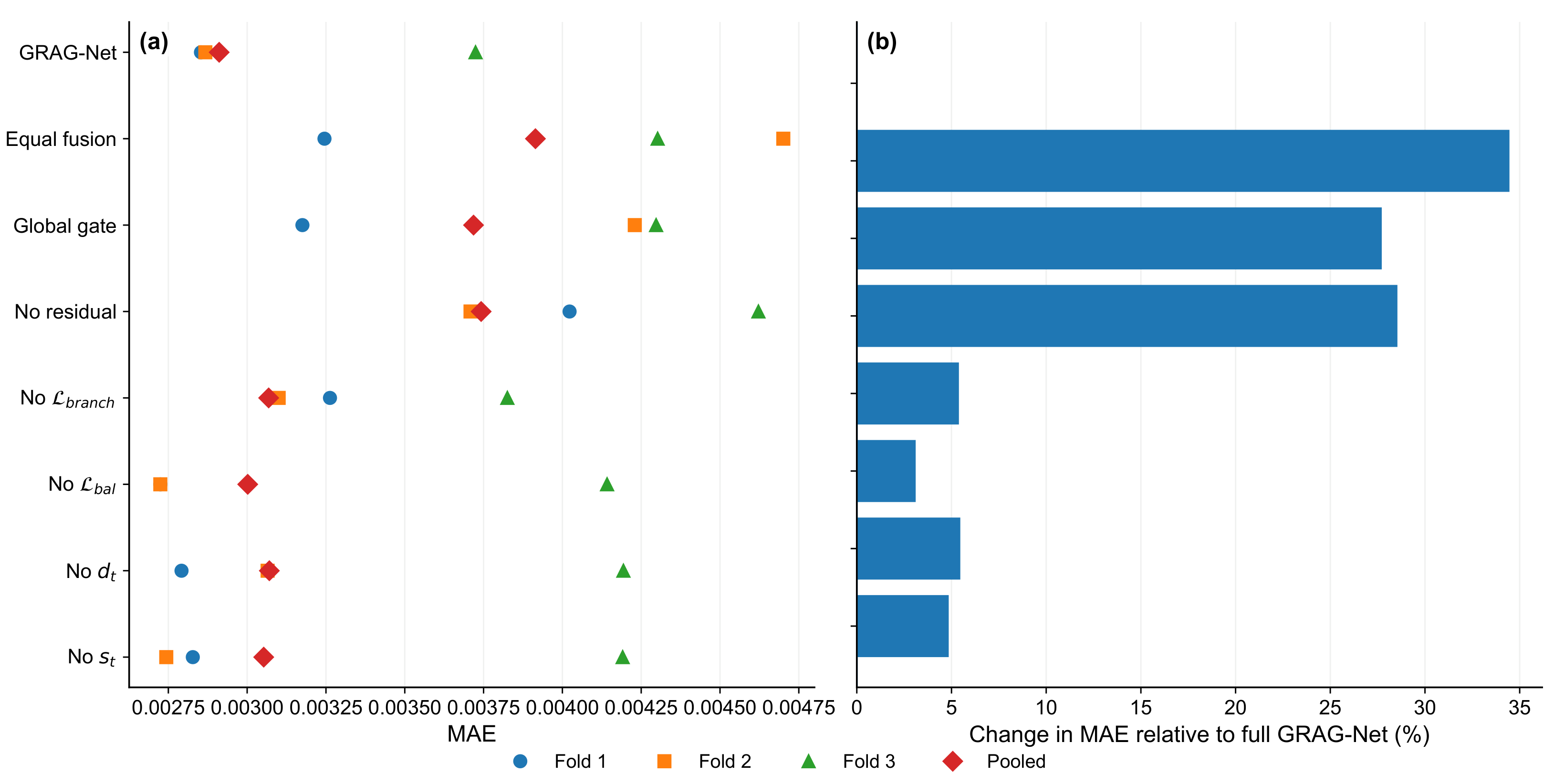
Figure 8 summarizes independently trained and re-optimized ablations. Relative to the full model’s pooled MAE of mole%, fixed equal fusion increases MAE by , a global gate by , and removal of residual reconstruction by . Removing branch supervision, disagreement, process-change context, or gate-balance regularization produces smaller pooled degradations of approximately 3–. The dominant performance losses therefore occur when the residual formulation or sample-dependent fusion mechanism is simplified, directly supporting the two central design choices of GRAG-Net.
Figure 8.
Formal independently trained ablations. (a) Fold-wise and pooled MAE. (b) Pooled percentage change in MAE relative to the full GRAG-Net. Positive values denote degradation relative to the full model.
The smaller components show more modest and fold-dependent effects and should be interpreted as regularizing or contextual refinements rather than as uniformly dominant mechanisms. In particular, the “no AR noise” row is a re-optimized control rather than evidence that perturbation itself is beneficial: the selected full-model configuration has , so autoregressive perturbation is inactive in the final GRAG-Net. This distinction prevents attributing a causal benefit to a component that was not used by the selected model.
3.5. Paired Moving-Block Bootstrap Evidence
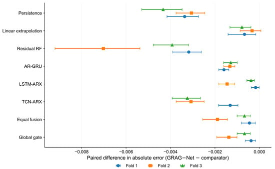
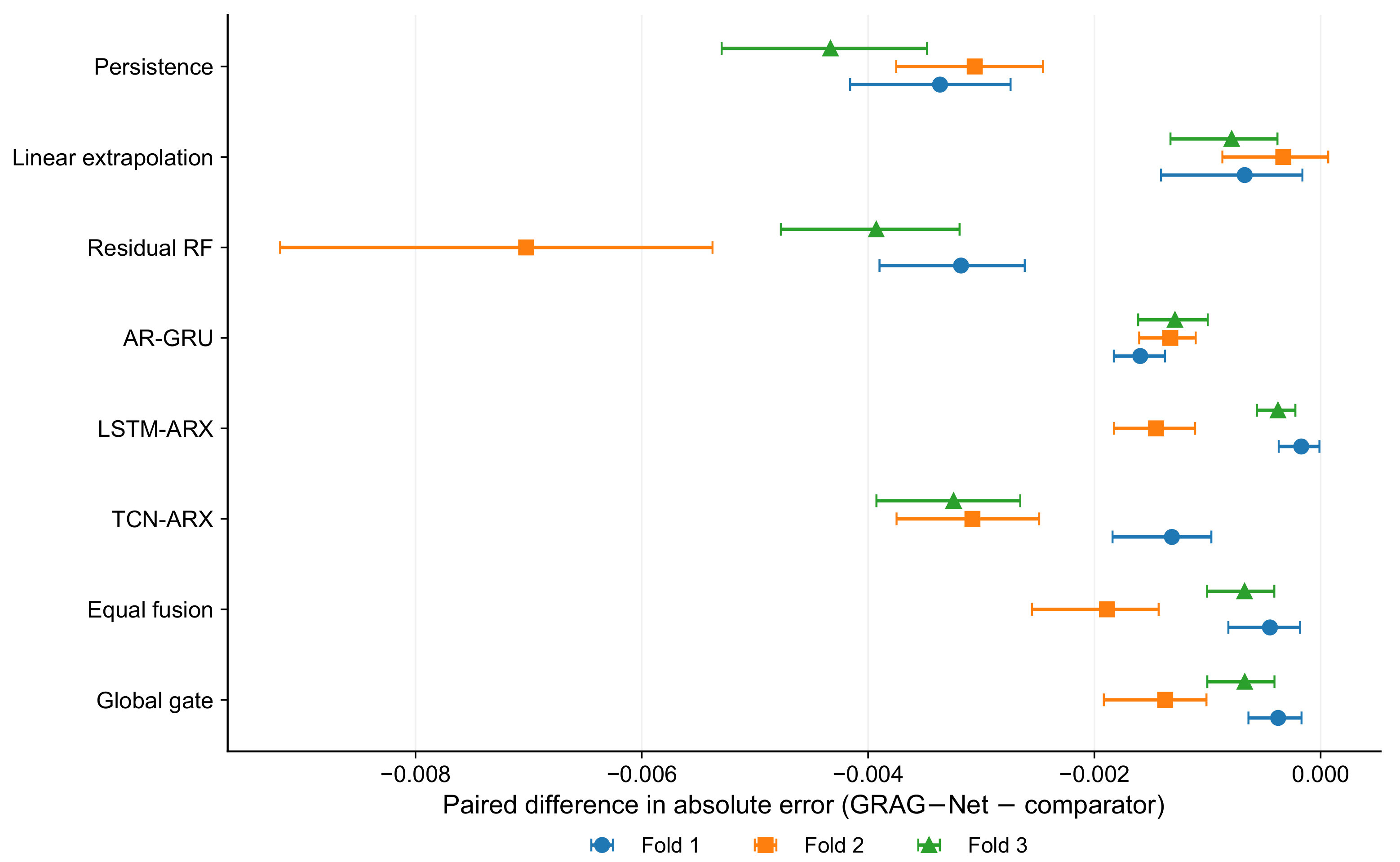
The paired moving-block bootstrap provides dependence-aware uncertainty for sample-wise error differences within each chronological test period. Figure 9 reports the primary 30-sample block analysis for absolute error, where negative values of favor GRAG-Net. Against AR–GRU, the mean differences are , , and mole% in Folds 1–3, and all three 95% confidence intervals lie entirely below zero. GRAG-Net is likewise favored in all folds against LSTM–ARX, TCN–ARX, equal fusion, global gating, persistence, residual RF, and residual SVR. Linear extrapolation is inferior in Folds 1 and 3, while its Fold 2 interval slightly overlaps zero.
Figure 9.
Paired moving-block bootstrap differences in absolute error for the primary block length of 30 samples. Each point is the mean of and the horizontal interval is the 95% bootstrap confidence interval. Negative values favor GRAG-Net.
This analysis strengthens the descriptive metric comparison because it preserves temporal pairing and serial dependence rather than treating individual time samples as independent. The conclusion is also insensitive to the alternative block lengths of 15 and 60 samples retained in the sensitivity analysis: the principal comparisons remain directionally consistent. Thus, the advantage of GRAG-Net over the strongest recurrent controls is not explained solely by averaging across seeds or by a small number of isolated test points.
3.6. Gate Behavior and Training-Only Temporal Lags
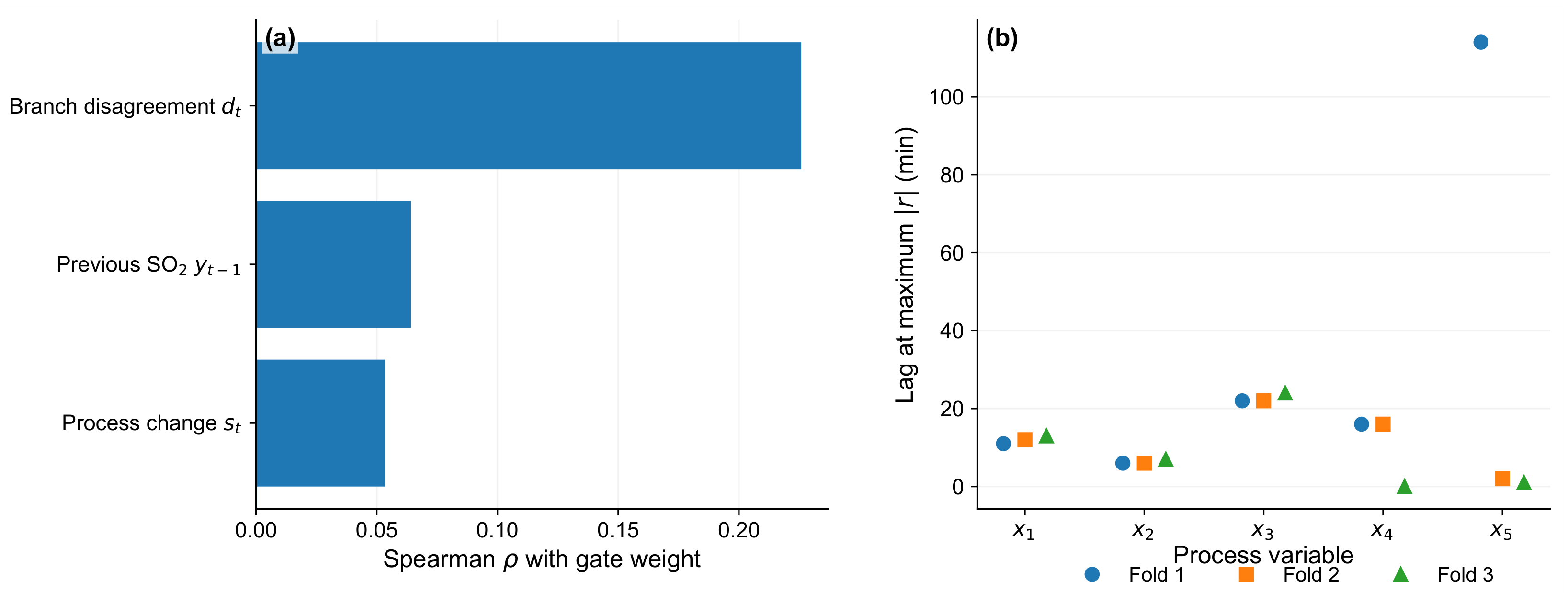
The inference-aware gate analysis in Figure 10a shows that the process-branch weight is most strongly associated with branch disagreement (), whereas associations with the process-change statistic () and the latest SO2 level () are weak. The gate should therefore be interpreted as a learned routing mechanism that reacts primarily to disagreement between the proposed process and autoregressive corrections, with weaker modulation by current process variation and target level. The retrospective association with realized process-branch advantage is only and is not treated as causal evidence because it depends on the subsequently observed target.
Figure 10.
Inference-aware gate and temporal-lag diagnostics. (a) Pooled Spearman association between gate weight and causal gate-context variables. (b) Training-only lag at maximum absolute process–SO2 correlation in each fold.
Training-only lag analysis in Figure 10b identifies the clearest delayed linear relationships for , , and , whose maximum absolute correlations generally occur about 6–24 min before the SO2 response. The corresponding values are modest (approximately –), indicating that no single process variable provides a dominant linear predictor. The Fold 1 maximum for occurs at 114 min but has only ; this weak boundary-like maximum is therefore not interpreted as a physically precise delay. The lag analysis supports the use of temporal process histories while reinforcing the need for a nonlinear multivariate representation.
3.7. SHAP Interpretation and Stability
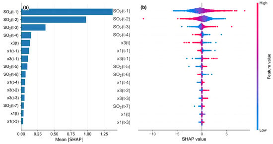
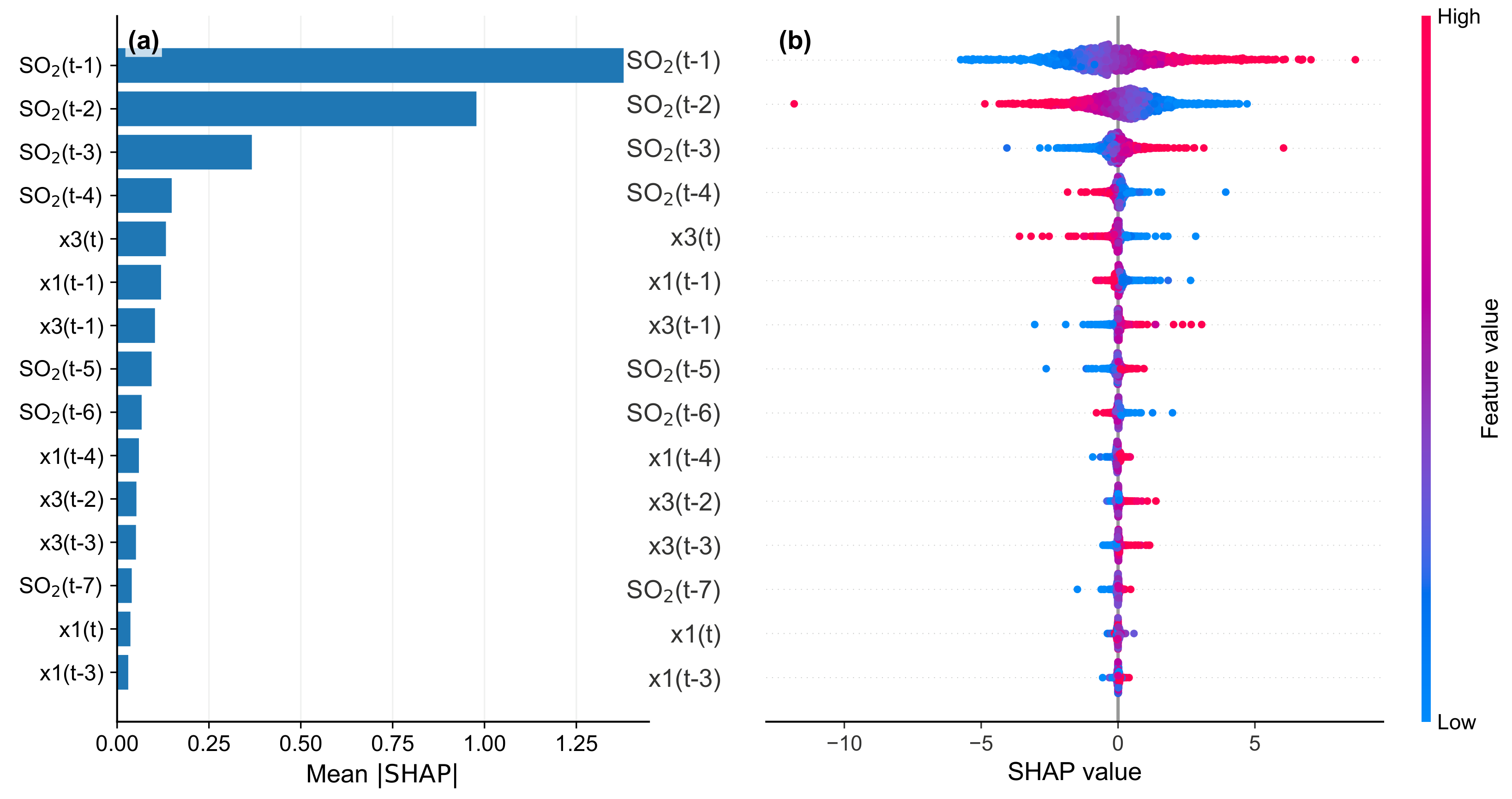
The aggregated SHAP analysis in Figure 11 confirms that recent SO2 history provides the dominant persistence information. The four highest-ranked features are through , with mean absolute SHAP values of , , , and , respectively. The strongest exogenous contributions are current , , and . This ordering is physically consistent with the architecture: the autoregressive branch supplies the dominant local baseline, while airflow histories provide complementary information for correcting the estimate.
Figure 11.
Aggregated SHAP interpretation of GRAG-Net. (a) Mean absolute SHAP importance for the 15 leading lagged features. (b) SHAP beeswarm showing the direction and magnitude of sample-level contributions.
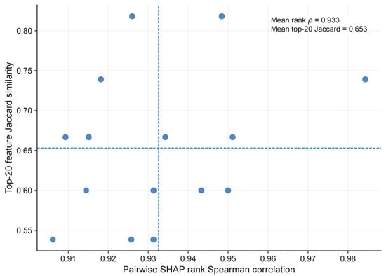
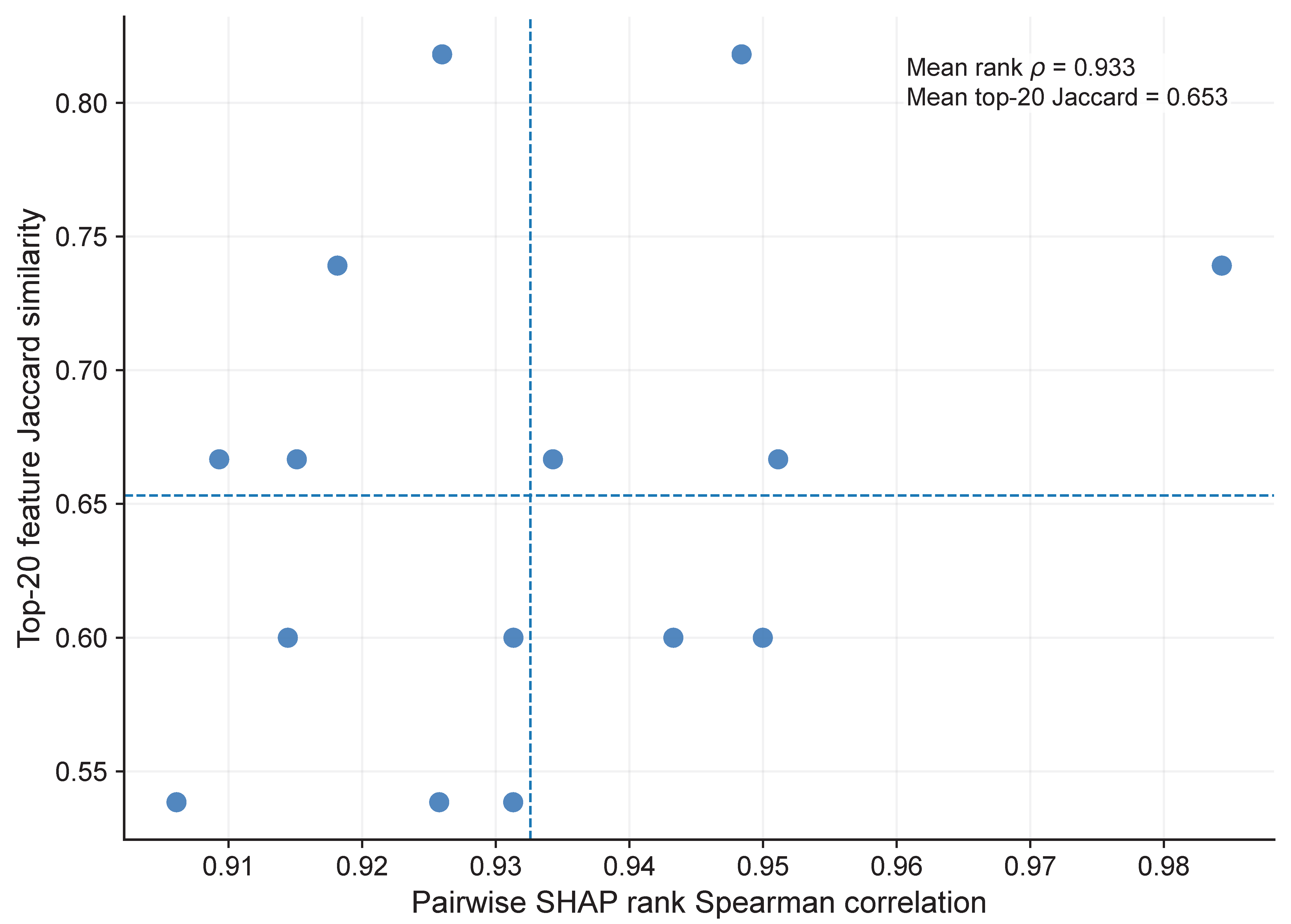
The beeswarm representation further indicates nonlinear and sample-dependent effects rather than a single fixed coefficient for each process lag. These attributions describe the fitted predictor and should not be interpreted as causal plant effects, particularly because neighboring lags and airflow channels are correlated. Importantly, the revision no longer relies on one fitted artifact. Across the six predefined fold–seed artifacts (three folds and seeds 42 and 52), the mean pairwise rank Spearman correlation is (range –), and the mean top-20 Jaccard overlap is (range –). The dominant feature ordering is therefore stable across chronological periods and random initialization, while lower-ranked features show the expected greater variability.
Figure 12 summarizes the consistency of SHAP feature rankings across folds and seeds using Spearman correlation and top-20 Jaccard overlap.
Figure 12.
Cross-fold and cross-seed stability of SHAP rankings. Each point compares two fitted artifacts using full-rank Spearman correlation and top-20 Jaccard overlap; dashed lines denote the corresponding means.
3.8. Error Reliability and Target-Change Regimes
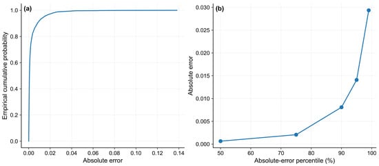
The error-reliability analysis in Figure 13 shows that GRAG-Net improves both the center and the upper tail of the error distribution relative to AR–GRU. Its median absolute error is mole%, compared with mole% for AR–GRU. At the 90th, 95th, and 99th percentiles, GRAG-Net errors are , , and mole%, whereas AR–GRU reaches , , and mole%, respectively. The performance gain is therefore not confined to a few extreme observations; it extends from typical errors through the upper tail.
Figure 13.
GRAG-Net error reliability. (a) Empirical CDF of absolute error. (b) Selected absolute-error percentiles, highlighting the concentration of typical errors and the upper tail.
The target-change analysis gives a complementary view. GRAG-Net attains MAE/RMSE of 0.00095/0.00210 mole% in the stable regime, 0.00243/0.00444 mole% in the changing regime, and 0.01465/0.02202 mole% during large changes. The corresponding AR–GRU values are 0.00131/0.00225, 0.00412/0.00553, and 0.02014/0.02690 mole%. GRAG-Net therefore outperforms the dedicated autoregressive recurrent model in all three regimes, with the largest absolute margin occurring during rapid target changes. This finding supports the intended role of the process branch: exogenous histories provide corrective information that is useful not only during transitions but also during routine one-step estimation.
Overall, the revised evidence is internally consistent across descriptive metrics, chronological folds, Taylor statistics, block-bootstrap intervals, formal ablations, and error-regime analysis. GRAG-Net does not obtain its advantage from target persistence alone: AR–GRU, linear extrapolation, and fixed/global fusion controls all remain weaker. Instead, the combination of residual reconstruction, separate process and autoregressive representations, and sample-dependent routing yields the most accurate and stable one-step predictions among the evaluated models. The gate, lag, and SHAP analyses further support a cautious mechanistic interpretation in which recent SO2 history provides the dominant baseline and process history supplies complementary corrections when the two predictive pathways disagree.
4. Conclusions and Future Work
This study developed GRAG-Net for causal rolling one-step SO2 soft sensing in an industrial sulfur recovery unit. The architecture separates exogenous process dynamics from autoregressive target persistence, predicts residual corrections relative to the latest measured SO2 value, and combines the two branches through a sample-dependent gate. The major revision strengthens the evidence for this design through three chronological future periods, five final seeds, stronger sequence and residual baselines, independently trained ablations, and dependence-aware moving-block bootstrap analysis.
Across the 15 descriptive fold–seed evaluations, GRAG-Net achieved MAE mole%, RMSE mole%, and , providing the strongest overall primary-metric performance among the evaluated full models. On pooled seed-ensemble predictions, MAE and RMSE were and mole%, representing reductions of and relative to persistence and and relative to AR–GRU. GRAG-Net also produced the lowest centered RMSE in all three Taylor folds, lower absolute-error quantiles from the median through the 99th percentile than AR–GRU, and lower MAE and RMSE in stable, changing, and large-change regimes. Paired moving-block bootstrap intervals favor GRAG-Net over AR–GRU in all three folds for absolute error, further supporting that the improvement is consistent within the chronological test periods rather than being driven by pooled averaging alone.
The formal ablations identify residual reconstruction and sample-dependent fusion as the principal architectural contributors: replacing dynamic routing with equal fusion, replacing it with a global gate, or removing residual reconstruction increases pooled MAE by approximately , , and , respectively. Auxiliary losses and individual gate-context variables have smaller and more fold-dependent effects. Inference-aware gate analysis shows that routing is associated most strongly with branch disagreement, while training-only lag analysis identifies modest delayed relationships for the principal airflow channels. Aggregated SHAP analysis confirms that recent SO2 lags dominate prediction and that process variables provide complementary exogenous information; the feature ranking remains stable across folds and seeds (mean rank ).
The conclusions remain limited to one publicly available SRU benchmark and to a rolling one-step setting in which measured SO2 history is available through . The study does not evaluate sustained analyzer outages, recursive multi-step prediction, cross-refinery transfer, or closed-loop deployment. Because the benchmark does not document analyzer accuracy or regulatory tolerance, the reported model errors are not interpreted as evidence of compliance with a particular hardware specification. Future work should prioritize external validation on additional SRUs, recursive outage-oriented evaluation, uncertainty calibration, drift-aware adaptation, and prospective deployment studies under documented analyzer specifications.
Funding
This research was funded by ongoing research funding program (ORF-2026-2179), King Saud University, Riyadh, Saudi Arabia.
Institutional Review Board Statement
Not applicable.
Informed Consent Statement
Not applicable.
Data Availability Statement
The industrial SRU dataset analyzed in this study is publicly available in Mendeley Data, Version 1, at https://doi.org/10.17632/6p865gztg6.1. A reproducibility package containing the source code used for the final reviewer experiments, chronological split definitions, preprocessing protocol, hyperparameter search spaces and selected configurations, epoch-selection records, final random seeds, fold–seed predictions, evaluation metrics, bootstrap outputs, ablation results, and interpretability-analysis files has been retained and is available from the corresponding author.
Conflicts of Interest
The author declares no conflicts of interest.
References
- Seinfeld, J.H.; Pandis, S.N. Atmospheric Chemistry and Physics: From Air Pollution to Climate Change, 3rd ed.; Wiley: Hoboken, NJ, USA, 2016. [Google Scholar]
- Lelieveld, J.; Evans, J.S.; Fnais, M.; Giannadaki, D.; Pozzer, A. The contribution of outdoor air pollution sources to premature mortality on a global scale. Nature 2015, 525, 367–371. [Google Scholar] [CrossRef] [Scilit] [PubMed]
- Fortuna, L.; Rizzo, A.; Sinatra, M.; Xibilia, M.G. Soft analyzers for a sulfur recovery unit. Control Eng. Pract. 2003, 11, 1491–1500. [Google Scholar] [CrossRef] [Scilit]
- Thameem, M.; Raj, A.; Berrouk, A.; Jaoude, M.A.; AlHammadi, A.A. Artificial intelligence-based forecasting model for incinerator in sulfur recovery units to predict SO2 emissions. Environ. Res. 2024, 249, 118329. [Google Scholar] [CrossRef] [Scilit] [PubMed]
- Quek, C.I.; Balasubramanian, R.; Rangaiah, G.P. Consider using ‘soft analyzers’ to improve SRU control. Hydrocarb. Process. 2000, 79, 101–106. [Google Scholar]
- Kadlec, P.; Gabrys, B.; Strandt, S. Data-driven soft sensors in the process industry. Comput. Chem. Eng. 2009, 33, 795–814. [Google Scholar] [CrossRef] [Scilit]
- Souza, F.A.A.; Araújo, R.; Mendes, J. Review of soft sensor methods for regression applications. Chemom. Intell. Lab. Syst. 2016, 152, 69–79. [Google Scholar] [CrossRef] [Scilit]
- Jiang, Y.; Yin, S.; Dong, J.; Kaynak, O. A review on soft sensors for monitoring, control, and optimization of industrial processes. IEEE Sens. J. 2021, 21, 12868–12881. [Google Scholar] [CrossRef] [Scilit]
- Kadlec, P.; Grbić, R.; Gabrys, B. Review of adaptation mechanisms for data-driven soft sensors. Comput. Chem. Eng. 2011, 35, 1–24. [Google Scholar] [CrossRef] [Scilit]
- Brunner, V.; Siegl, M.; Geier, D.; Becker, T. Challenges in the development of soft sensors for bioprocesses: A critical review. Front. Bioeng. Biotechnol. 2021, 9, 722202. [Google Scholar] [CrossRef] [Scilit] [PubMed]
- Bolf, N.; Mohler, I.; Golob, M.; Galinec, G.; Ivandić, M. Software sensor for sulphur recovery unit control. Chem. Eng. Trans. 2009, 17, 1191–1196. [Google Scholar]
- Bidar, B.; Shahraki, F.; Sadeghi, J.; Khalilipour, M.M. Soft sensor modeling based on multi-state-dependent parameter models and application for quality monitoring in industrial sulfur recovery process. IEEE Sens. J. 2018, 18, 4583–4591. [Google Scholar] [CrossRef] [Scilit]
- Yuan, X.; Wang, Y.; Yang, C.; Gui, W. Stacked isomorphic autoencoder based soft analyzer and its application to sulfur recovery unit. Inf. Sci. 2020, 534, 72–84. [Google Scholar] [CrossRef] [Scilit]
- Patanè, L.; Xibilia, M.G. Echo-state networks for soft sensor design in an SRU process. Inf. Sci. 2021, 566, 195–214. [Google Scholar] [CrossRef] [Scilit]
- Curreri, F.; Patanè, L.; Xibilia, M.G. RNN- and LSTM-based soft sensors transferability for an industrial process. Sensors 2021, 21, 823. [Google Scholar] [CrossRef] [Scilit] [PubMed]
- Mou, T.; Liu, J.; Zou, Y.; Li, S.; Xibilia, M.G. Enhanced industrial process modeling with transfer-incremental-learning: A parallel SAE approach and its application to a sulfur recovery unit. Control Eng. Pract. 2024, 148, 105955. [Google Scholar] [CrossRef] [Scilit]
- Wang, Q.; Li, L. Research on semi-supervised soft sensor modeling method for sulfur recovery unit based on ISSA-VMD-ESN. Chem. Eng. Sci. 2024, 298, 120397. [Google Scholar] [CrossRef] [Scilit]
- Sun, W.; Li, L.; Lu, B.; Jiang, L.; Zhang, J. Hybrid multiscale forecasting of SRU sulfur gas concentrations using VMD, CEEMDAN and optimized PatchTST. iScience 2026, 29, 114986. [Google Scholar] [CrossRef] [Scilit] [PubMed]
- Li, J.; Hao, Y. Dynamic soft sensor model based on combination of GRU and TCN–Transformer for chemical process application. J. Meas. Sci. Instrum. 2026, 17, 171–182. [Google Scholar] [CrossRef] [Scilit]
- Cerqueira, V.; Torgo, L.; Mozetič, I. Evaluating time series forecasting models: An empirical study on performance estimation methods. Mach. Learn. 2020, 109, 1997–2028. [Google Scholar] [CrossRef] [Scilit]
- Huber, P.J. Robust estimation of a location parameter. Ann. Math. Stat. 1964, 35, 73–101. [Google Scholar] [CrossRef] [Scilit]
- Sun, W. Industrial Sulfur Gas Concentration Dataset for SRU Forecasting. In Mendeley Data; Version 1; Elsevier: Amsterdam, The Netherlands, 2026. [Google Scholar] [CrossRef]
- Drucker, H.; Burges, C.J.C.; Kaufman, L.; Smola, A.; Vapnik, V. Support vector regression machines. Adv. Neural Inf. Process. Syst. 1997, 9, 155–161. [Google Scholar]
- Breiman, L. Random forests. Mach. Learn. 2001, 45, 5–32. [Google Scholar] [CrossRef] [Scilit]
- Geurts, P.; Ernst, D.; Wehenkel, L. Extremely randomized trees. Mach. Learn. 2006, 63, 3–42. [Google Scholar] [CrossRef] [Scilit]
- Chen, T.; Guestrin, C. XGBoost: A scalable tree boosting system. In Proceedings of the 22nd ACM SIGKDD International Conference on Knowledge Discovery and Data Mining, San Francisco, CA, USA, 13–17 August 2016; Association for Computing Machinery: New York, NY, USA, 2016; pp. 785–794. [Google Scholar] [CrossRef] [Scilit]
- Bergmeir, C.; Hyndman, R.J.; Koo, B. A note on the validity of cross-validation for evaluating autoregressive time series prediction. Comput. Stat. Data Anal. 2018, 120, 70–83. [Google Scholar] [CrossRef] [Scilit]
- Akiba, T.; Sano, S.; Yanase, T.; Ohta, T.; Koyama, M. Optuna: A next-generation hyperparameter optimization framework. In Proceedings of the 25th ACM SIGKDD International Conference on Knowledge Discovery and Data Mining, Anchorage, AK, USA, 4–8 August 2019; Association for Computing Machinery: New York, NY, USA, 2019; pp. 2623–2631. [Google Scholar] [CrossRef] [Scilit]
- Taylor, K.E. Summarizing multiple aspects of model performance in a single diagram. J. Geophys. Res. Atmos. 2001, 106, 7183–7192. [Google Scholar] [CrossRef] [Scilit]
- Lundberg, S.M.; Lee, S.-I. A unified approach to interpreting model predictions. Adv. Neural Inf. Process. Syst. 2017, 30, 4765–4774. [Google Scholar]
- Cao, L.; Ji, X.; Cao, Y.; Li, Y.; Siang, L.C.; Li, J.; Pediredla, V.K.; Gopaluni, R.B. Interpretable soft sensors using extremely randomized trees and SHAP. IFAC-PapersOnLine 2023, 56, 8000–8005. [Google Scholar] [CrossRef] [Scilit]

Disclaimer/Publisher’s Note: The statements, opinions and data contained in all publications are solely those of the individual author(s) and contributor(s) and not of MDPI and/or the editor(s). MDPI and/or the editor(s) disclaim responsibility for any injury to people or property resulting from any ideas, methods, instructions or products referred to in the content. |
© 2026 by the author. Licensee MDPI, Basel, Switzerland. This article is an open access article distributed under the terms and conditions of the Creative Commons Attribution (CC BY) license.