


Abstract
Climate and land-cover change can alter where birds find suitable environmental conditions, raising the question of which areas may remain suitable across plausible futures. We addressed this question in the Yangtze River Basin, China, using pooled bird occurrence records from 6209 occupied 1 km grid cells. We combined three presence–background models using climate, elevation and land-cover predictors. The ensemble achieved a mean area under the receiver operating characteristic curve of 0.752 across the outer folds of nested spatial cross-validation. Across six joint climate and land-cover scenarios classified using mean ranks from three climate models, gains above the fixed baseline 25th-percentile cutoff covered approximately 122,000–147,000 km2 and exceeded losses of 36,000–81,000 km2. At the baseline median cutoff, the joint candidate area shared by all 18 future combinations covered approximately 1840 km2 under the stricter environmental-support criterion (NN95) and 61,600 km2 under the more permissive criterion (NN99). Hubei and Jiangsu ranked among the three provinces with the largest candidate areas under both criteria, joined by Hunan under NN95 and Sichuan under NN99. These spatial contrasts can guide coordinated field assessments and inform habitat retention and urban blue–green infrastructure planning.
1. Introduction
Climate change alters the conditions under which organisms obtain resources, reproduce and survive, challenging conservation strategies based on current habitat distributions [1]. Protected habitats may become less climatically suitable, while sites outside protected areas may acquire favourable conditions [2,3,4,5,6,7,8]. Conservation planning therefore needs to consider where suitable conditions may persist, decline or emerge. Distribution models address this question by relating biological records to environmental conditions and projecting these associations under future scenarios [2]. In urban planning, areas that remain suitable across alternative futures may help identify priorities for habitat retention. Climate-refugia assessments provide a framework for evaluating such persistence, provided that modelled suitability is distinguished from demonstrated ecological persistence [3,4,5].
Some bird groups can indicate habitat conditions relevant to urban planning. Waterbirds, for example, respond to seasonal water regimes and shoreline habitat, whereas responses to vegetation and disturbance vary among terrestrial species [9,10,11,12,13]. Habitat composition and management influence the bird assemblages supported by cities, and responses to blue–green spaces vary among groups [10,14,15]. These relationships make bird data relevant to decisions concerning vegetation, water bodies and habitat mosaics. Bird population indicators also provide established tools for tracking conservation outcomes [16].
The Yangtze River Basin contains closely connected aquatic, terrestrial and urban landscapes. Floodplain lakes, rivers and wetlands provide feeding, breeding, stopover and wintering habitats for waterbirds and other migratory birds. Studies of the basin document environmental influences on waterbird communities and identify habitat networks of conservation importance [11,12,13]. Forests, agricultural land and urban vegetation support other bird groups. Cities and infrastructure are concentrated along parts of the river corridor and around lakes, where development can transform these habitats. The extensive modification of Yangtze Plain lakes illustrates this pressure [17]. Conservation planning must therefore account for connections between river–lake habitats and neighbouring terrestrial and urban areas.
Climatic suitability and habitat availability constrain conservation opportunities in different ways. Seasonal temperature and rainfall influence environmental suitability, while land conversion changes vegetation, water cover and disturbance. Cities can support biodiversity where sufficient space and appropriate habitat structures remain [18,19]. Both land-cover composition and vertical habitat structure influence urban bird communities [20,21]. Climatic suitability alone therefore cannot establish habitat value. Planning must also consider whether habitat resources remain available in persistent areas, whether pressures can be managed in declining areas, and whether newly suitable areas are accessible to the species concerned [22,23,24,25].
Identifying potential refugia also requires attention to the spatial scale and ecological mechanisms of persistence [25,26]. At the basin scale, intersecting projections can reveal a shared geographical core obscured by aggregate area estimates. Summarising these patterns by province can inform coordination across administrative boundaries, particularly in connected river–lake systems. Site-level decisions still require information on species, habitat condition and human activities.
Previous species-level distribution projections and Yangtze waterbird assessments address potential range shifts and important habitats [6,7,8,13]. We compare changes in pooled bird-record scores across the basin and use climate-model agreement and environmental support to identify candidate sites for field assessment. This comparison complements species-level habitat assessments and protected-area planning, which address different conservation outcomes [27,28,29,30,31,32]. Recent research has examined wetland and habitat-quality dynamics in the middle basin [33], climate-related changes in protected-area effectiveness in the middle and lower basin [34], and protected-area expansion for biodiversity and ecosystem services in the Yangtze River Economic Belt [35]. Our analysis tests how restricting projections to environments similar to those used for model fitting changes the area and location of candidate sites.
2. Materials and Methods
2.1. Study Area
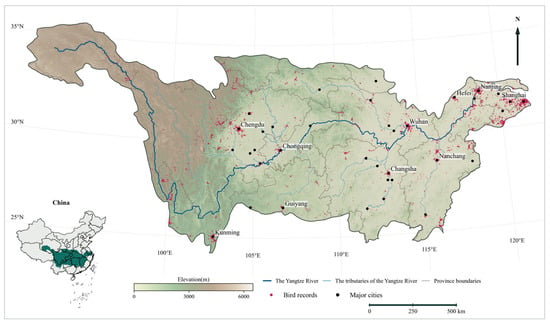
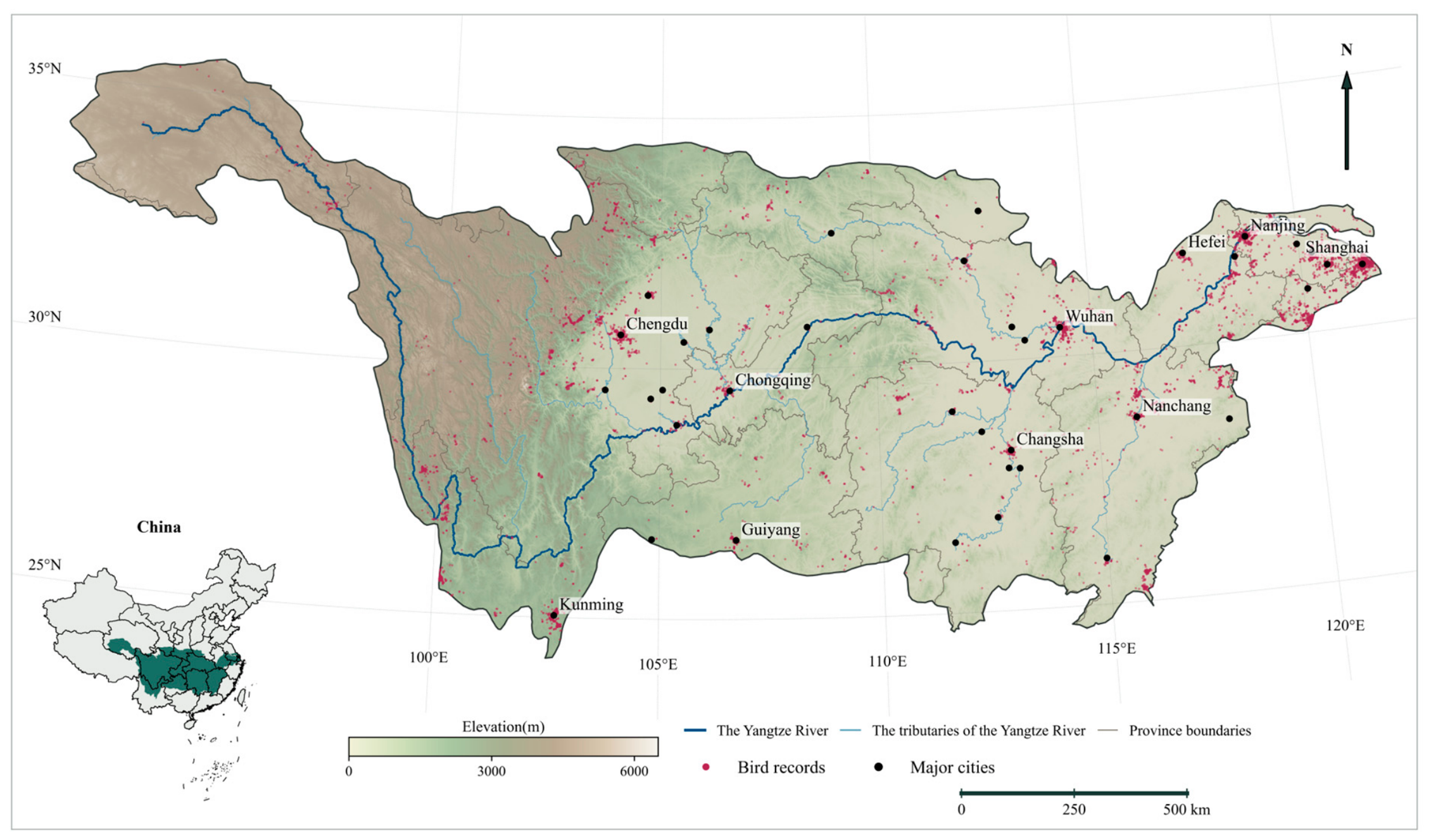
The Yangtze River Basin extends from the Qinghai–Tibet Plateau to the East China Sea, covering approximately 1.8 million km2 [36], or about 18.8% of China’s land area [37] (Figure 1). The basin supports a wide range of species across its forests, grasslands, rivers, lakes and wetlands, with forests covering more than 41% of the basin. Representative conservation taxa include Chinese sturgeon (Acipenser sinensis), Yangtze finless porpoise (Neophocaena asiaeorientalis), Chinese alligator (Alligator sinensis), giant panda (Ailuropoda melanoleuca), golden snub-nosed monkey (Rhinopithecus roxellana), Chinese silver fir (Cathaya argyrophylla), dawn redwood (Metasequoia glyptostroboides) and dove tree (Davidia involucrata Baill.) [38]. River–lake habitats provide feeding, breeding, stopover and wintering resources for different bird groups [11,13]. Urban development along the river brings these habitats into close proximity to expanding settlements and infrastructure, increasing conservation pressures.
Figure 1.
Yangtze River Basin and bird occurrence records.
2.2. Bird Occurrence Records and Processing
2.2.1. Occurrence Data Collection
Broad distributions, established identification methods and documented responses to environmental change support the use of birds in biodiversity monitoring [9,16]. Relative suitability describes the environmental associations of pooled bird records [9,16]. Floodplain lakes, rivers and wetlands support waterbirds and migrants in the Yangtze River Basin, whereas terrestrial and urban vegetation supports other bird groups [11,13,17]. Vegetation structure, land cover and blue–green habitats also influence bird responses within cities [10,14,20,21]. We therefore included water, forest and impervious-cover variables to represent aquatic, wooded and developed environments without assuming that all recorded species depend on wetlands. The dataset comprised public occurrence records from 2015 to 2025, pooled across species and seasons.
2.2.2. Occurrence Quality Control and Environmental Coverage
Public bird occurrence records dated 2015–2025 were retrieved from the Global Biodiversity Information Facility (GBIF) (https://www.gbif.org/; accessed on 4 July 2026). Quality control excluded duplicate identifiers, invalid coordinates or dates, records outside the basin, records indicating absence or non-positive counts, records explicitly identified as captive or managed, and records with generalised coordinates. Records were required to have reported coordinate uncertainty greater than zero and no greater than 1000 m; a value of zero was not interpreted as exact positioning. Coordinate checks incorporated record metadata and followed established occurrence-cleaning principles [39]. Of 72,912 retrieved records, 48,873 passed quality control, representing 706 species-level taxon identifiers. After pooling species and seasons, we retained one presence per occupied 1 km × 1 km equal-area cell to reduce within-cell duplication [40]. This yielded 6212 occupied cells, of which 6209 had complete values for the retained predictors and were included in modelling. We sampled 50,000 background cells with selection probabilities proportional to their areas [41]. Area-weighted background sampling represents the environments available within the basin. Uneven observation effort among cells can persist after spatial thinning and affect spatial cross-validation. We audited GBIF dataset identifiers, record types, years and the number of occupied 1 km cells and 100 km blocks. To test dependence on source composition, we refitted quadratic logistic regression using only cells represented in the dominant iNaturalist dataset, retaining the full-model specification and background sample. We compared the upper baseline quartiles, defined separately with area-weighted scores, using area-weighted intersection over union and overlap with joint NN95 persistence candidates.
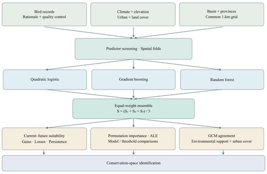
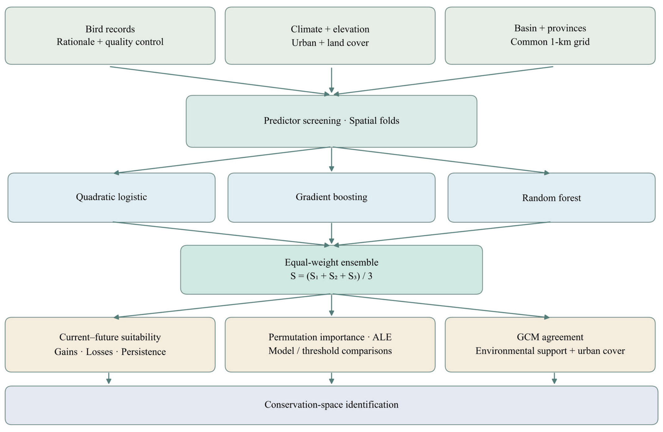
We aggregated bird records to a 1 km grid and screened environmental predictors for redundancy. We evaluated quadratic logistic regression, histogram gradient boosting and random forests by spatial cross-validation and averaged their scores with equal weights. We used permutation importance and fitted response curves to examine predictor contributions to discrimination and fitted associations. We then compared baseline and future relative-suitability maps to quantify changes in area and class membership, locate areas of agreement across climate models and assess their overlap with impervious cover (Figure 2).
Figure 2.
Workflow for screening candidate bird conservation areas.
2.3. Environmental Variables and Processing
2.3.1. Bioclimatic Variables
We considered all nineteen WorldClim 2.1 bioclimatic variables (BIO1–BIO19), encompassing temperature conditions, seasonality and precipitation (https://www.worldclim.org/). Baseline climate data represented 1970–2000 at a native resolution of 30 arcseconds. Future climate projections were obtained from three global climate models (GCMs), ACCESS-CM2, BCC-CSM2-MR and MIROC6, under three Shared Socioeconomic Pathway (SSP) and radiative forcing combinations, SSP1-2.6, SSP2-4.5 and SSP5-8.5, for 2041–2060 and 2061–2080. These models were selected to compare distinct climate-model configurations using consistently downscaled products available for all selected pathways and periods. Published descriptions and evaluations document differences in model structure and simulated climate, including East Asian circulation in BCC-CSM2-MR and western Pacific precipitation in MIROC6 [42,43,44]. Current and future projections used the same screened bioclimatic variables.
2.3.2. Additional Variables
Additional predictors characterised environmental attributes relevant to bird occurrence: elevation represented the topographic setting; water and forest fractions represented aquatic and wooded cover; cropland fraction represented agricultural cover; and impervious cover represented urban development [10,11,14,20,21]. Elevation was held constant over the projection horizon, consistent with its treatment in climate–habitat modelling [6,7]. Baseline impervious cover represented 2015, and baseline land cover represented 2020; SSP-linked projections for 2050 and 2070 provided future values for urban, forest, water and cropland cover [45,46]. The 1970–2000 climate normal, 2015 impervious map and 2020 land-cover map are a composite reference for records from 2015 to 2025, not a contemporaneous reconstruction. The analysis therefore assumes that this reference adequately describes broad environmental contrasts over the occurrence period.
2.3.3. Harmonisation and Variable Screening
Candidate predictors comprised BIO1–BIO19; elevation; impervious-surface percentage; and forest, water and cropland fractions. We assumed that the fitted environmental associations remained applicable despite differences among baseline periods. Climate and elevation data at a native resolution of 30 arcseconds were harmonised with land-cover data at 1 km resolution on a 1 km equal-area grid. Continuous values were area-averaged; land-cover classes were converted to binary indicators before averaging. Unclassified land-cover values coded as zero were excluded, and basin-edge weights were calculated from polygon–cell intersections. Basin-wide Pearson correlations, weighted by the area of each cell within the basin, were calculated independently of the bird response. Elevation was given priority in the fixed candidate order. A candidate was excluded if its absolute Pearson correlation with any previously retained predictor was at least 0.8. This procedure reduced pairwise predictor redundancy [47]. The same retained predictor set was used to fit the models and generate baseline and future projections (Table 1).
Table 1.
Retained predictors and data sources.
2.4. Modelling Relative Environmental Suitability
2.4.1. Model Fitting and Ensemble Construction
We fitted quadratic logistic regression (QL), histogram gradient boosting (HGB) and random forests (RF) using scikit-learn 1.9.1 in Python 3.12.14. Each algorithm produced a presence–background classification score. Predictors for QL were standardised within each training set. Two hyperparameter configurations per algorithm were compared using three-fold grouped cross-validation within each outer training set. We evaluated predictive performance in four outer folds defined by geographical clusters of 100 km spatial blocks, with a 20 km buffer between training and test locations. Performance was assessed using the area under the receiver operating characteristic curve (ROC AUC) and average precision, recognising that these metrics are affected by the presence and background sampling design [2,27,28,48,49,50,51,52]. The final models were refitted after validation.
For reproducibility, logistic regression used standardisation followed by quadratic polynomial features, class balancing, a maximum of 1500 iterations, and C ∈ {0.1, 1}. Histogram gradient boosting used 150 iterations, a learning rate of 0.06, a minimum of 40 samples per leaf, an L2 penalty of 10, no early stopping, and maximum numbers of leaf nodes ∈ {15, 31}. Random forests used 200 trees, a minimum of 15 samples per leaf, a maximum feature fraction of 0.7 per split, class balancing, and maximum tree depths ∈ {12, 20}. Hyperparameters for each algorithm were selected by mean inner-fold AUC. Ensemble weights were fixed independently of outer-fold performance. The ensemble score was the arithmetic mean of the three algorithm scores, S = (Slogistic + Sboosting + Sforest)/3. Higher scores indicate greater modelled similarity to environments associated with recorded presences relative to the sampled background [2,29,41].
2.4.2. Nested Spatial Validation
The four outer test folds comprised geographical clusters of 100 km blocks. In each iteration, one region was held out, and training locations within 20 km of its test locations were excluded. Hyperparameters were selected by three-fold grouped cross-validation within the remaining training data, with buffered separation also imposed in the inner folds. AUC and average precision quantify presence–background discrimination and are affected by the composition of the presence and background samples. The study-specific performance criteria required a mean outer-fold ensemble AUC ≥ 0.70 and AUC ≥ 0.65 in at least three of the four outer folds [27,28,50,51,52]. The discrimination thresholds are descriptive benchmarks, not evidence of ecological calibration or adequate performance throughout the basin or in future conditions. Using the same buffered spatial splits, we excluded each test fold when fitting the scaler and nearest-neighbour support rules, applied the training-only range and distance checks to test environments, and calculated the fraction passing both checks. We also recombined saved out-of-fold scores into the three possible equal-weight two-algorithm ensembles and compared their discrimination. This comparison assesses how algorithm choice affects out-of-fold discrimination.
2.4.3. Future Projections and Suitability Classes
Three GCMs, three SSP–forcing combinations, and two periods yielded eighteen future combinations. Climate projections for 2041–2060 and 2061–2080 were paired with land-cover projections for 2050 and 2070, respectively. The main projections changed climate and land-cover variables jointly, while climate-only comparisons retained baseline land cover; elevation remained fixed in both cases. Before prediction, inputs outside the fitted training ranges were clamped to the nearest range boundary. Because classification thresholds can affect area estimates, we explicitly defined the classes and examined alternative thresholds [53,54]. Scores were converted to area-weighted percentile ranks using the baseline cumulative distribution function (CDF). Ranks < 0.25, 0.25 to <0.50, 0.50 to <0.75 and ≥0.75 defined the unsuitable, low, moderate and high relative-suitability classes, respectively. These operational classes are not independently validated ecological boundaries. The quartile cutoffs were defined using the original basin-wide modelling domain. We applied those cutoffs and fitted models to the provincial reporting domain, where baseline class areas can differ from 25% of the domain. The same baseline CDF was applied to all future projections, allowing future class areas to change. For each SSP–period combination, the main future map was obtained by averaging the three GCM rank maps and classifying the resulting mean. Each GCM map was also classified separately. The suitable area obtained by classifying a GCM-mean rank map therefore need not equal the mean suitable area obtained by classifying each GCM map separately. Individual-algorithm comparisons used each algorithm’s own baseline CDF, held fixed for future predictions. At rank ≥ 0.25, approximately three quarters of the baseline area falls above the cutoff by construction, subject to ties and masking. We refer to this as the above-cutoff class, not as an independently delineated ecological range. Rank ≥ 0.50 selects the upper half of the reference score distribution for the more selective persistence screen.
2.4.4. Predictor Response Analysis
Accumulated local effects (ALE) summarised fitted predictor responses. Within each predictor bin, model scores were evaluated at the lower and upper bin boundaries while the other sampled predictor values were retained; mean local differences were then accumulated and centred. Curves were calculated from classification scores before baseline-rank transformation [55]. ALE calculations used 5000 area-weighted draws with replacement from baseline cells, a random seed of 20261020 and up to 20 quantile bins. Duplicate boundaries were removed, yielding fewer bins for land-cover fractions with many zero values. The ensemble curve was the mean of the separately centred algorithm curves. ALE describes fitted associations rather than causal effects [55]. Predictive importance was quantified as the decrease in held-out ROC AUC after shuffling one predictor within an outer test region while retaining the original training buffer and selected hyperparameters [27,48]. Each predictor was shuffled five times per fold, using a random seed of 20261021 plus the fold index. AUC decreases were averaged first across permutations within each fold and then equally across the four folds. Models refitted for response analysis reproduced the original fold AUCs. Positive importance indicates that shuffling impaired discrimination; negative values indicate higher AUC after permutation.
2.5. Suitability Change and Potential Persistence
2.5.1. Area Accounting and Suitability Transitions
The primary suitable set comprised the low, moderate and high classes (rank ≥ 0.25). Gain was defined as a transition from below threshold to suitable, loss as the reverse transition, stable suitability as meeting the threshold under baseline and future conditions, and stable below-threshold status as meeting it under neither baseline nor future conditions. Gain minus loss therefore equals future minus current suitable area. A separate 4 × 4 matrix recorded transitions among all four classes; a cell could remain suitable while moving between the low, moderate and high classes. Areas were summed using exact fractional polygon–cell intersections within the basin portion of each province. Gain, loss and net-change percentages used current suitable area as the denominator; basin shares used the common valid prediction domain. Thresholds of 0.50 and 0.75 were used for sensitivity comparisons.
2.5.2. Potential Persistence and Environmental Support
We used nearest-neighbour distances to assess how closely projected conditions resembled the environments used for model fitting. Predictors were standardised, and Euclidean distance to the nearest unique training-environment vector was calculated. The NN95 criterion used the 95th percentile of leave-one-out nearest-neighbour distances among unique training vectors as its cutoff; NN99 used the 99th percentile. Support also required every original, unclamped future predictor to remain within its univariate training range. Potential climatic refugia were defined as cells with a current rank ≥ 0.50 and ranks ≥ 0.50 in all three future climate-only GCM projections that also met the environmental-support criteria. Land-cover variables retained baseline values in these projections. Joint persistent areas were identified by applying the same criteria to projections in which both climate and land cover changed. Consensus was evaluated separately for each SSP–period combination. The six consensus maps, each requiring agreement among three GCMs, were then intersected to identify the common core across all eighteen future combinations. These maps indicate potential persistence at baseline and during the two future periods; they do not demonstrate uninterrupted suitability between those periods. Provincial shares used the sum of the corresponding provincial persistent areas as the denominator. Contiguous patches defined by four-neighbour connectivity and their area-weighted centroids characterised spatial concentration. Persistence intersections requiring unanimous GCM agreement were evaluated both with and without environmental-support restrictions. Baseline urban overlap was also calculated for the persistence intersections across all eighteen combinations, using impervious cover ≥ 10% to identify overlap with baseline developed settings. The leave-one-out distance quantiles are internal reference cutoffs, not validation against an independent baseline sample. The univariate rule detects marginal range violations; the distance rule can also flag unusual predictor combinations within marginal ranges. A prediction flagged by either rule remains uncertain even when its fitted score is high. We centred each predictor at its mean and scaled it by its population standard deviation in the final presence–background training sample before deduplicating standardised vectors. Euclidean distances were unweighted. NN95 is the stricter operational proximity screen, used to flag a conservative candidate subset rather than selected as an empirically optimal boundary. To evaluate spatial sensitivity, we applied rank cutoffs of 0.25, 0.50 and 0.75 to baseline and every joint future member under both support rules and ranked provinces by retained area using the same fractional area weights.
2.5.3. Mapping Candidate Conservation and Survey Areas
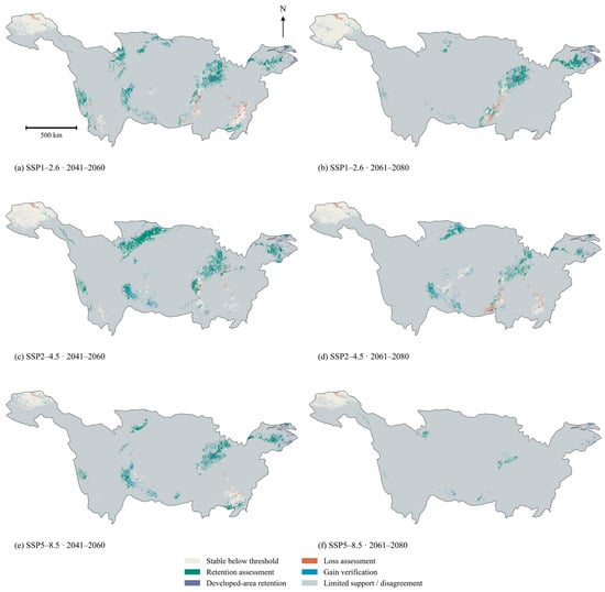
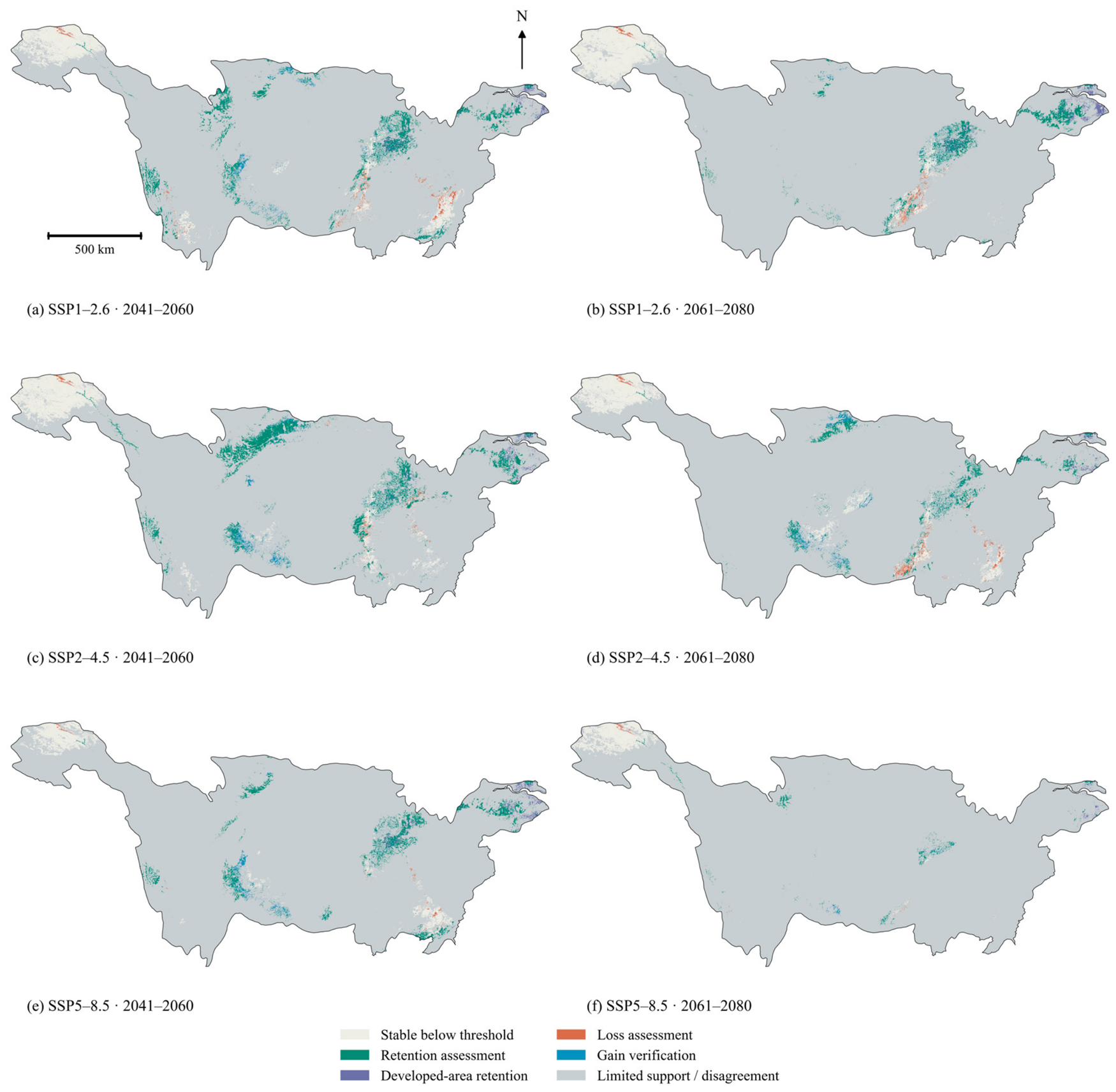
For each SSP–period combination, we combined current suitability, unanimous outcomes across the three GCMs, environmental support and future impervious cover. Supported cells with rank ≥ 0.50 under current conditions and in all three future GCM projections were mapped as candidate habitat-retention areas, subdivided into settings with lower impervious cover (<10%) and developed settings (≥10%). For this conservation screening, the same rank threshold of 0.50 defined all change categories, distinct from the 0.25 threshold used for the main suitable-area analysis. Among supported cells, loss required current rank ≥ 0.50 and future rank < 0.50 in all three GCMs; gain required current rank < 0.50 and future rank ≥ 0.50 in all three GCMs. Stable below-threshold cells had current rank < 0.50 and future rank < 0.50 in all three GCMs. Loss and gain identified candidates for restoration assessment and habitat-resource verification, respectively. The two retention categories, loss, gain and stable below-threshold categories were mutually exclusive. All other cells in the common valid domain were assigned to a single residual category comprising limited environmental support or GCM disagreement, so the six mapped categories partitioned the entire domain. The 10% impervious-cover cutoff was a spatial screening convention rather than a biological response threshold.
2.5.4. Sensitivity of Projected Expansion
Suitable-area change was assessed for each GCM and statistical algorithm at fixed baseline-rank thresholds of 0.25, 0.50 and 0.75. Counts of increases and decreases summarised agreement among configurations. To assess sensitivity to environmental support, current and future areas were recalculated within the same paired domains, defined by univariate training ranges and the additional NN95 or NN99 proximity criterion. In eighteen additional projections, impervious cover was held at baseline values while climate and forest, water and cropland fractions took their future values; the fitted models and baseline ensemble CDF were unchanged.
3. Results
3.1. Predictor Screening, Model Performance and Predictor Responses
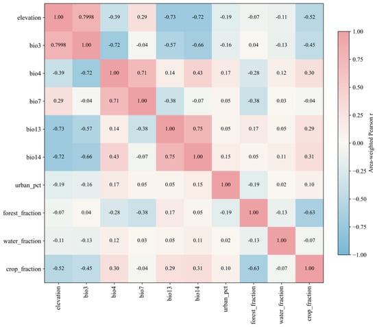
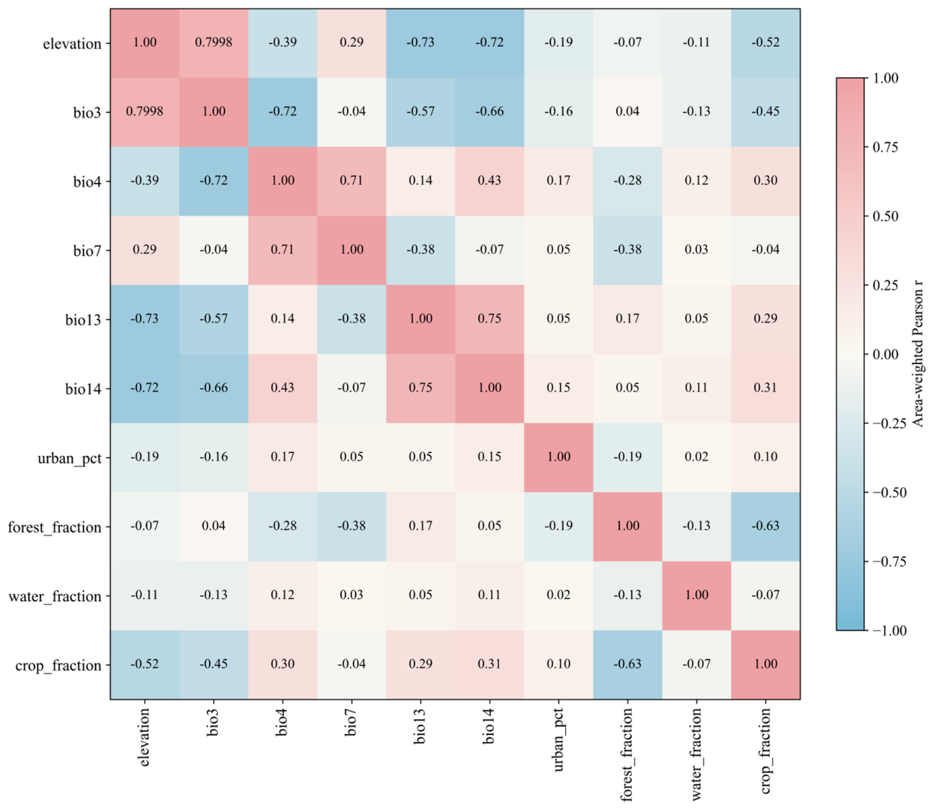
Correlation screening retained 10 of the 24 candidate predictors: elevation, five bioclimatic variables (BIO3, BIO4, BIO7, BIO13 and BIO14), and four land-cover variables (impervious, forest, water and cropland cover; Table 1). Figure 3 shows the area-weighted Pearson correlations among the retained predictors. The maximum absolute pairwise correlation was 0.7998, just below the 0.8 exclusion threshold. The correlation matrix for all 24 candidates is presented in Figure S1.
Figure 3.
Correlations among the ten retained environmental predictors.
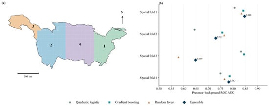
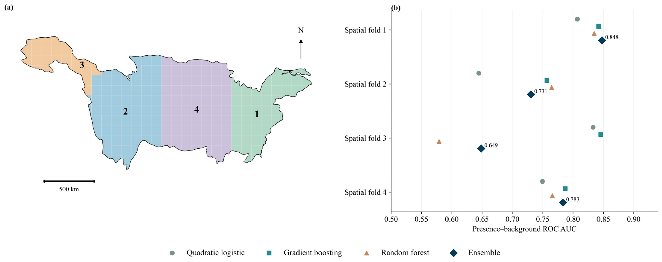
The ensemble achieved a mean outer-fold AUC of 0.752 and a mean average precision of 0.399. The four fold-specific AUCs were 0.848, 0.731, 0.649 and 0.783 (Figure 4). The mean AUC exceeded 0.70, and three of the four folds met the AUC benchmark of 0.65. In the third fold, which covered the north-western test region, AUC was 0.579 for random forest and 0.845 for gradient boosting (Figure 4). Urban cells (baseline impervious cover ≥ 10%) and cells containing mapped water (water fraction > 0) accounted for 49.81% and 16.91% of presence cells, respectively, compared with 5.35% and 3.60% of the modelled area. Both conditions were met in 8.36% of presence cells.
Figure 4.
Spatial cross-validation folds (a) and model performance (b).
The upper-quartile baseline areas from the full-record and iNaturalist-restricted quadratic logistic models had an area-weighted intersection over union of 0.864. Urban cells accounted for 20.9% and 21.0% of these areas, respectively. The proportion of the joint NN95 candidate area falling within each model’s upper-quartile baseline area was 31.1% and 32.6%, respectively. The north-western test fold contained 81 presence and 5077 background samples, with a median elevation of 4683 m compared with 599 m in its buffered training sample. Across the four held-out folds, 14.8–36.7% of samples met both the univariate range and NN95 proximity criteria, compared with 30.9–69.2% when NN99 was used. The two-algorithm ensembles had mean AUCs of 0.729–0.795 across the four folds and AUCs of 0.580–0.844 in the north-western fold.
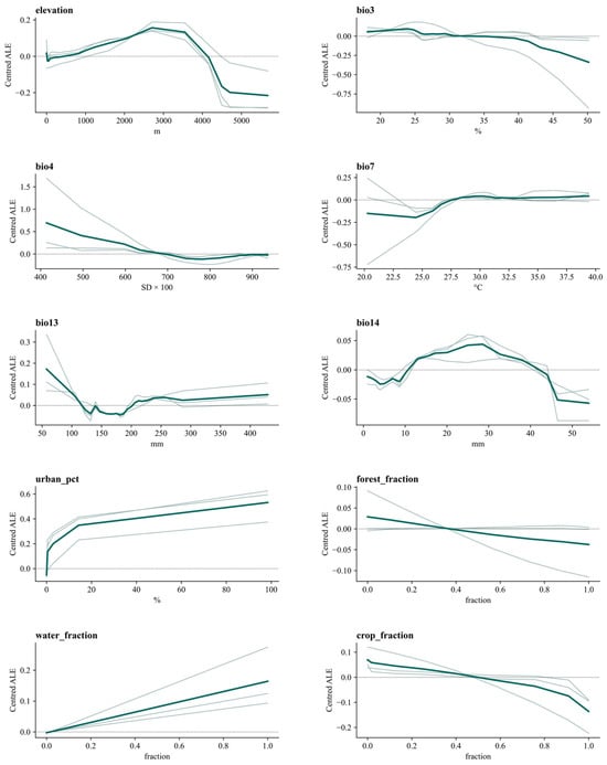
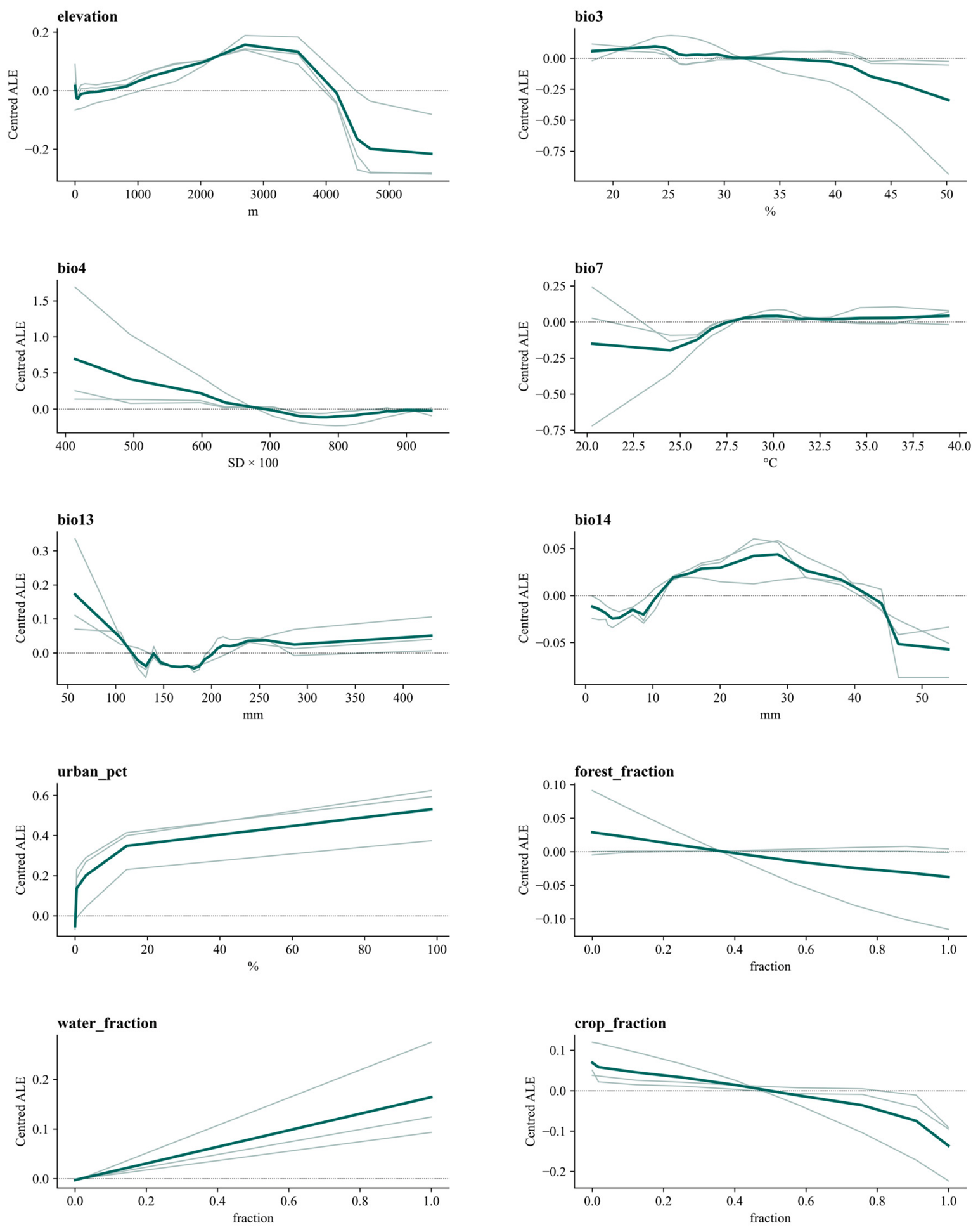
Ensemble ALE increased with impervious cover and water fraction. The elevation response peaked at intermediate elevations, whereas the forest and cropland responses decreased over parts of their observed ranges. Climatic responses differed among algorithms, particularly near the limits of predictor ranges. Curves for land-cover fractions had fewer segments where quantile boundaries coincided (Figure 5).
Figure 5.
Accumulated local effects of the fitted models. Green indicates the equally weighted ensemble; grey indicates individual model fits.
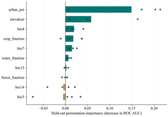
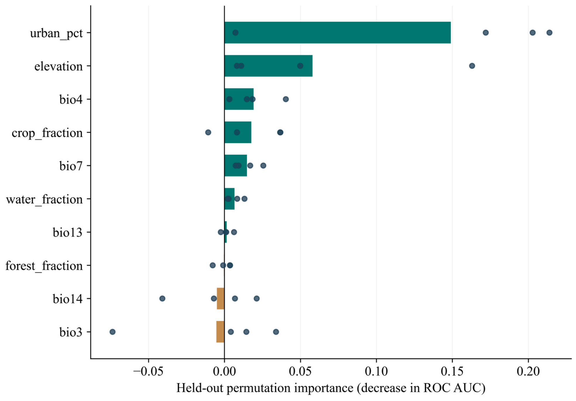
Held-out permutation importance was greatest for impervious cover (mean AUC decrease: 0.149), followed by elevation (0.058), BIO4 (0.019), cropland fraction (0.018) and BIO7 (0.015). Water fraction and BIO13 had mean AUC decreases of 0.007 and 0.001, respectively, whereas mean values for BIO3, BIO14 and forest fraction were negative. Importance varied among the four test regions (Figure 6).
Figure 6.
Spatially held-out permutation importance. Bars show the mean decrease in ensemble ROC AUC across four folds; points show fold means over five permutations. Negative values are retained.
3.2. Baseline Relative Suitability and Area Above the Cutoff
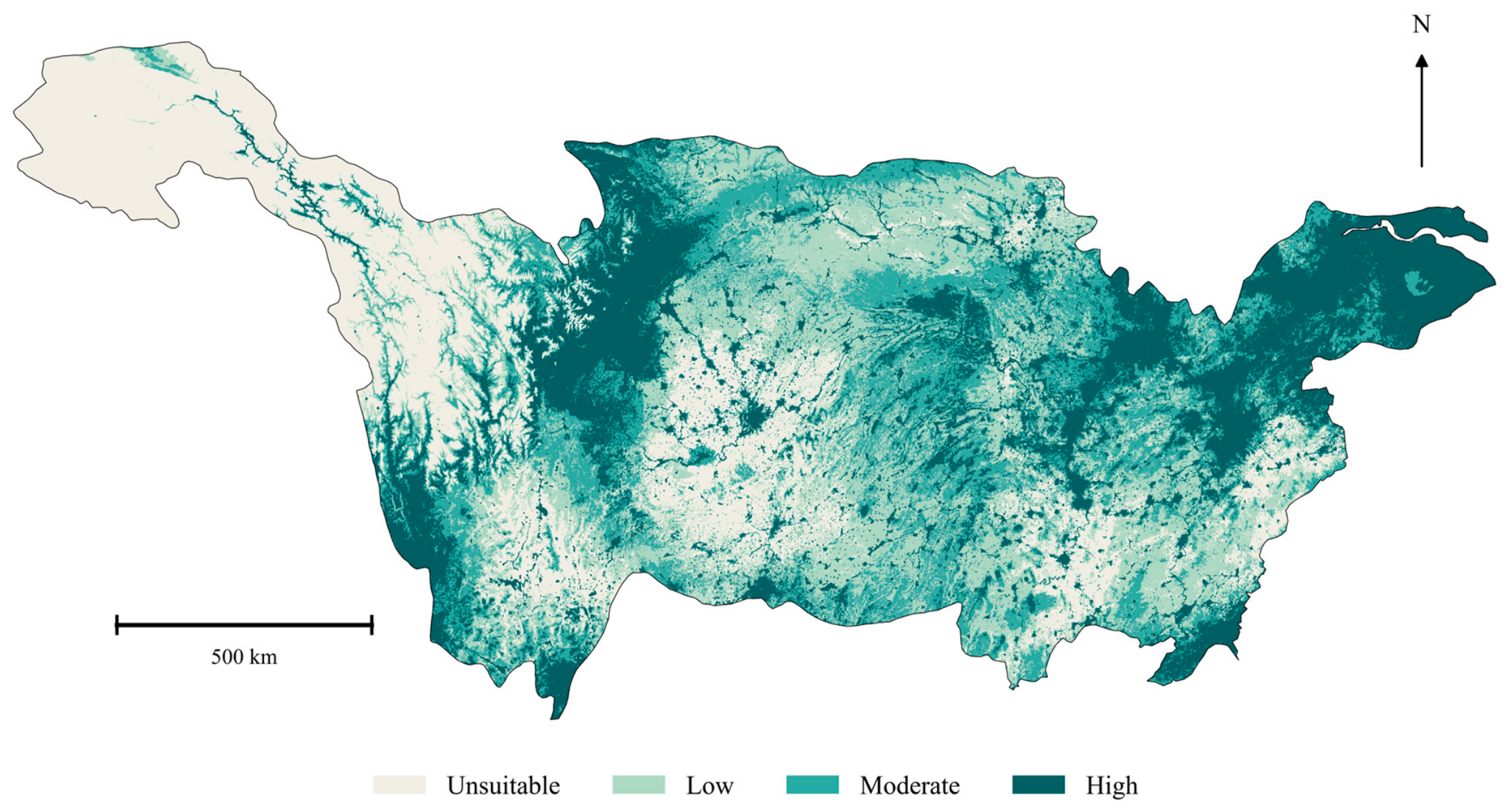
Current suitable area, defined as the upper three baseline classes, totalled 1,335,219.45 km2 (Figure 7). Sichuan had the largest current suitable area (308,753.20 km2), followed by Hubei (180,006.26 km2), Hunan (175,526.39 km2) and Jiangxi (139,138.01 km2). Suitable areas in Guizhou and Yunnan were 89,030.17 and 98,057.70 km2, respectively, while those in Jiangsu and Shanghai were 35,764.39 and 4247.52 km2 (Table 2).
Figure 7.
Current relative suitability for pooled bird occurrences.
Table 2.
Current and future suitable areas (km2) *.
3.3. Projected Relative Suitability and Area Above the Cutoff
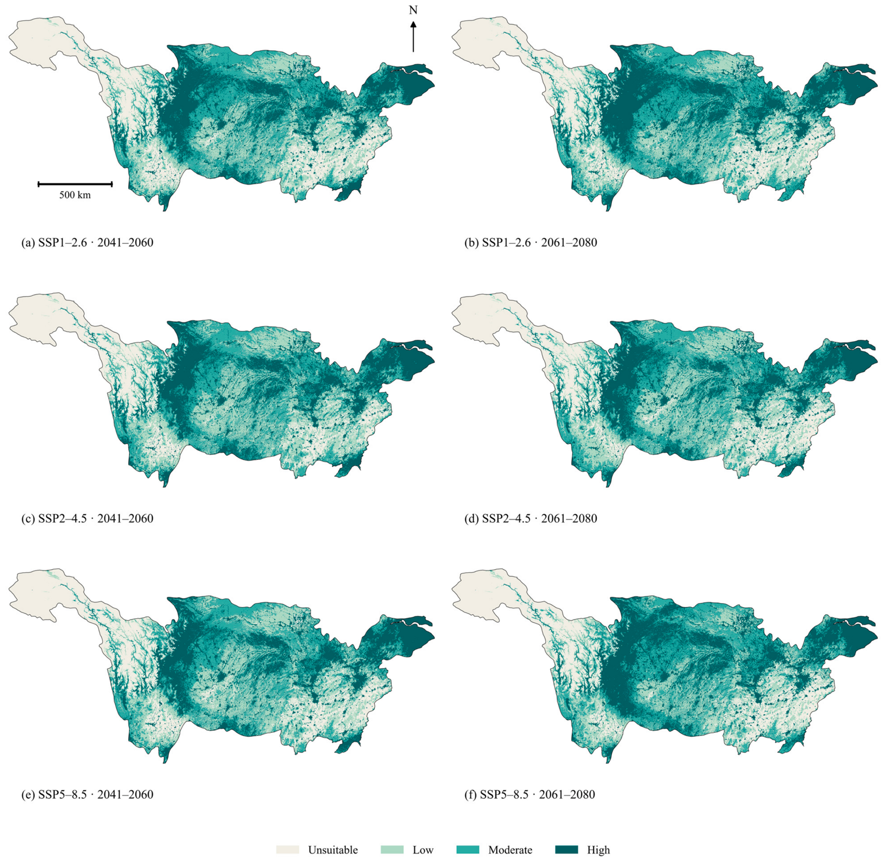
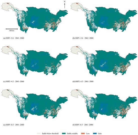
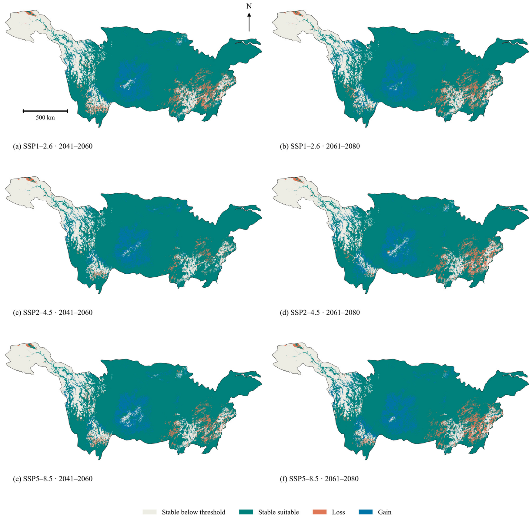
Future suitable area in the joint projections classified from GCM-mean ranks ranged from 1,377,342.93 to 1,433,257.48 km2, equivalent to 77.36–80.51% of the provincial reporting domain. Under SSP1-2.6, suitable area increased from 1,377,342.93 km2 in 2041–2060 to 1,397,746.85 km2 in 2061–2080. Under SSP2-4.5, it decreased from 1,433,257.48 to 1,402,034.70 km2; under SSP5-8.5, it increased from 1,395,321.06 to 1,402,900.04 km2. High-suitability areas in 2041–2060 were 480,275.96, 474,481.75 and 447,486.03 km2 under SSP1-2.6, SSP2-4.5 and SSP5-8.5, respectively. The corresponding areas in 2061–2080 were 522,771.09, 451,825.49 and 520,467.77 km2 (Figure 8).
Figure 8.
Future suitability under joint scenarios. (a,b) SSP1-2.6; (c,d) SSP2-4.5; (e,f) SSP5-8.5.
Sichuan retained the largest future suitable area (346,387.19–366,128.34 km2). Relative to current conditions, suitable area increased under all six SSP–period combinations in Sichuan, Guizhou and Chongqing, but decreased under all six in Hunan, Jiangxi and Qinghai. Suitable area in Jiangxi declined from 139,138.01 km2 to 98,295.20–126,901.04 km2, while that in Hunan declined from 175,526.39 to 155,082.67–170,758.05 km2. Jiangsu and Shanghai retained 35,764.39 and 4247.52 km2, respectively, in every SSP–period combination classified from GCM-mean ranks (Table 2). The centroid of the combined moderate- and high-suitability area shifted 56.65 km north-west under SSP1-2.6 in 2041–2060.
Across the eighteen GCM–SSP–period projections, high-suitability area ranged from 257,700.33 to 669,168.90 km2 for QL, from 436,122.01 to 577,002.00 km2 for HGB, and from 506,263.21 to 672,961.12 km2 for RF. Table 3 and Table 4 summarise GCM-specific ensemble areas and means of separately classified GCM areas for each algorithm, respectively. At rank ≥ 0.25, suitable area increased in 15 of the 18 GCM-specific ensemble projections and decreased in three; net changes ranged from −3.15% to 5.99%. Figure S2 summarises sensitivity to model choice and suitability thresholds.
Table 3.
Relative-suitability class areas by GCM, SSP–forcing combination and period (km2).
Table 4.
Mean relative-suitability class areas across GCMs for each statistical algorithm (km2).
3.4. Projected Gains, Losses and Suitability Transitions
Across the six joint scenarios classified from GCM-mean ranks, suitable-area gains ranged from 121,777.23 to 147,261.82 km2 and losses from 36,433.43 to 80,541.38 km2, while 1,254,678.07–1,298,786.02 km2 remained suitable. Gains exceeded losses in every scenario, yielding net gains of 42,123.48–98,038.03 km2 (3.15–7.34% of current suitable area) (Table 5 and Figure 9). Transitions among the four suitability classes comprised upgrades, downgrades and unchanged classes, distinguishing shifts within the suitable set from gains and losses across the suitability threshold (Table 6).
Table 5.
Suitable-area gains, losses, stability and net change (km2).
Figure 9.
Gains, losses and stability of suitable area.
Table 6.
Transitions among the four relative-suitability classes (km2).
3.5. Areas of Persistent Relative Suitability
Under the primary NN95 support criterion, the area of potential climatic refugia shared by all three GCMs decreased from 75,403.29 to 54,514.61 km2 between 2041–2060 and 2061–2080 under SSP1-2.6; from 87,036.23 to 44,915.35 km2 under SSP2-4.5; and from 61,364.23 to 10,731.12 km2 under SSP5-8.5. Joint persistent areas were smaller in all six comparisons, ranging from 7919.04 to 80,362.94 km2 (Table 7). The climate-only intersection across all eighteen future combinations covered 2806.49 km2. Jiangsu contributed 1041.49 km2 (37.11%), Hubei 949.47 km2 (33.83%) and Hunan 479.53 km2 (17.09%), together accounting for 88.03% of the climate-only intersection. Qinghai contributed a further 199.00 km2 (7.09%). Under joint climate and land-cover change, the common persistent area across all eighteen combinations was 1836.95 km2. Hubei, Jiangsu and Hunan accounted for 655.68 km2 (35.69%), 482.95 km2 (26.29%) and 382.32 km2 (20.81%), respectively (Table 8). At the 0.50 cutoff, the leading provinces under NN95 were Hubei, Jiangsu and Hunan; under NN99 they were Hubei, Sichuan and Jiangsu. At the 0.25, 0.50 and 0.75 cutoffs, joint candidate areas were approximately 4209, 1837 and 503 km2 under NN95, and 111,280, 61,593 and 26,084 km2 under NN99. Hubei led at the two lower cutoffs under both support rules, whereas Jiangsu led at 0.75.
Table 7.
Supported three-GCM climatic refugia and joint persistence by scenario (km2).
Table 8.
Provincial distribution of supported persistent areas across all eighteen future combinations.
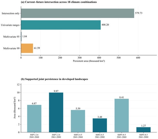
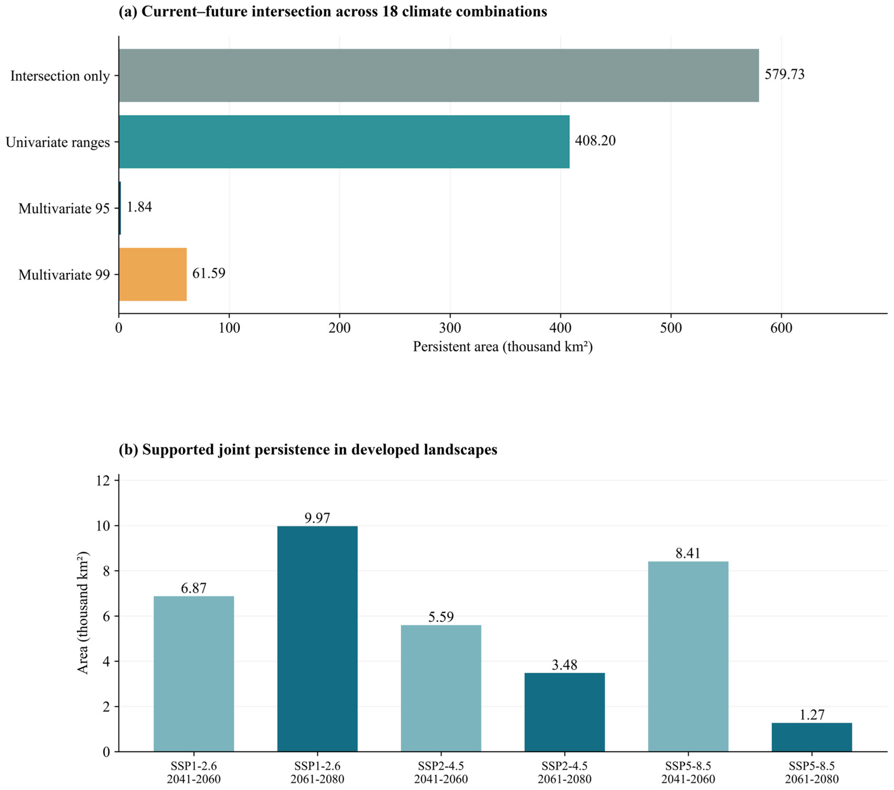
The largest patch of persistent relative suitability under climate-only change, defined by four-neighbour connectivity, covered 844.16 km2 in eastern Jiangsu. Other large patches occurred in Hubei (99.00 and 85.00 km2), Hunan (78.00 km2) and Qinghai (50.00 km2). Under joint change, the largest patch covered 324.67 km2 in eastern Jiangsu, followed by a 63.00 km2 patch in Hunan. Without environmental-support restrictions, intersections across all eighteen future combinations covered 575,045.15 km2 under climate-only change and 579,726.16 km2 under joint change. The NN99 support criterion retained 71,464.30 and 61,592.73 km2, respectively (Figure 10).
Figure 10.
Persistent relative suitability and urban overlap. (a) Intersection of current and joint future suitability across three GCMs × three SSP–forcing combinations × two periods within the provincial reporting domain under alternative support rules; (b) joint persistence across three GCMs that met the environmental-support criterion and overlapped cells with projected impervious cover ≥ 10%.
3.6. Overlap with Impervious Cover and Candidate Areas for Field Assessment
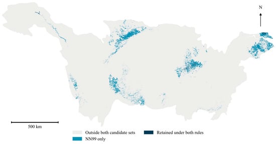
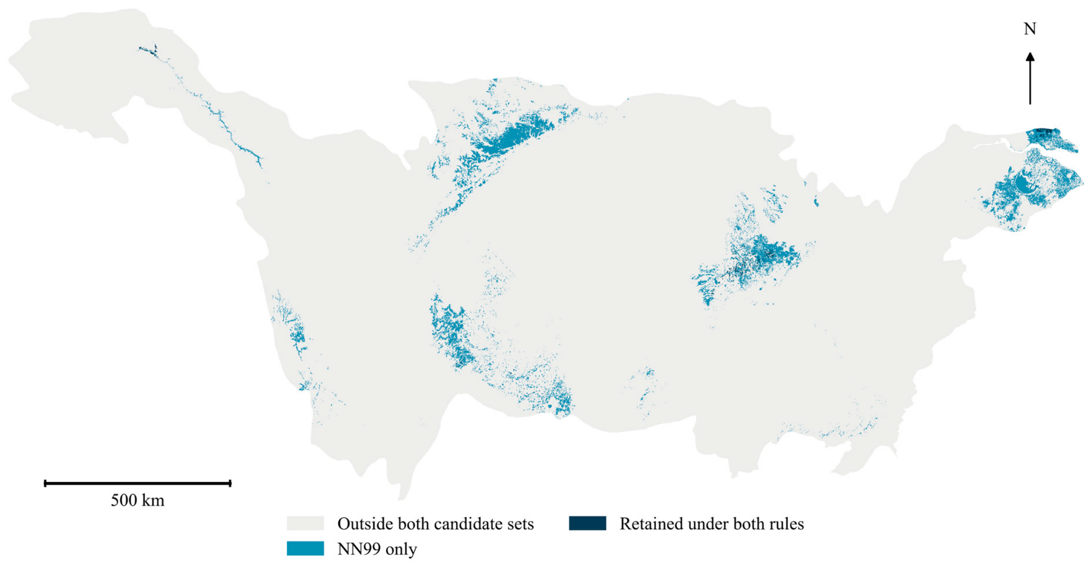
Across the six SSP–period combinations, supported areas of persistent suitability overlapping future impervious cover ≥ 10% ranged from 1269.96 to 9969.44 km2. In the intersection across all eighteen future combinations, 414.94 km2 of climate-only refugia and 54.70 km2 of joint persistent areas overlapped baseline impervious cover ≥ 10%. All overlap with the joint persistence intersection occurred in Jiangsu. The spatial classification distinguished candidate habitat-retention areas in settings with lower impervious cover and developed settings, restoration-assessment areas with unanimous losses, and newly suitable areas with unanimous gains. Cells with limited environmental support or GCM disagreement were mapped separately. The primary joint environmental-support domain covered 3.47–14.12% of the common prediction domain (Figure 11). Figure 12 compares the spatial distribution of joint candidate persistence under NN95 and NN99 at a relative-rank cutoff of 0.50, distinguishing areas retained under both rules from those retained only under NN99.
Figure 11.
Candidate areas for habitat retention, restoration assessment and field surveys.
Figure 12.
Spatial comparison of joint candidate persistence under NN95 and NN99 at relative rank ≥ 0.50.
4. Discussion
An increase in suitability for pooled bird occurrences does not imply a gain in biodiversity. Previous studies project range expansion for many Chinese birds but contraction for others [56], including substantial losses among protected species [57]. Forest recovery has also been associated with projected habitat expansion for non-migratory forest birds [58]. In our analysis, relative suitability for pooled occurrences could increase in environments associated with widespread or urban-tolerant species even as specialists lose habitat. The basin-wide balance of gains and losses should therefore be interpreted alongside the spatial distribution of decline and persistence, rather than as evidence of improved conservation status.
4.1. Current Suitability and Possible Mechanisms
The positive fitted response to water fraction is consistent with the feeding and resting resources provided by river–lake habitats. Its modest permutation importance indicates that water fraction contributed less to held-out discrimination than impervious cover or elevation. Water extent does not capture prey availability, shoreline vegetation or seasonal inundation, all of which may influence habitat use. Studies of floodplain waterbirds document the importance of habitat conditions and their temporal variation [11,12]. The response peak at intermediate elevations may reflect associations with climate and habitat heterogeneity, as terrain can create environmental contrasts over short distances [59]. Urban bird responses also vary among habitats and ecological groups [10,60,61]. Although impervious cover had the greatest permutation importance, its positive fitted response does not demonstrate an ecological benefit of urbanisation. Accessible urban sites may attract both urban-tolerant birds and observers, and area-weighted background sampling does not correct uneven observation effort [41]. The pooled records and area-weighted background sample cannot disentangle these ecological and sampling effects.
4.2. Interpreting Net Expansion and Suitability Redistribution
Seasonal temperature and precipitation may alter water availability, vegetation productivity and resource timing, while land-cover change modifies the spatial distribution of these resources. These processes could contribute to the contrasting provincial projections, but the fitted associations do not establish causal effects. Mean-temperature variables were excluded during screening, so projected expansion cannot be attributed directly to warming. The direction of change also depended on the algorithm and environmental-support criterion: at rank ≥ 0.25, suitable area increased in 15 of the 18 ensemble combinations, compared with five for QL, eight for HGB and eighteen for RF. Only ten ensemble combinations showed increases within paired NN95 domains. Projected net expansion is therefore conditional on modelling choices and the environments in which projections are evaluated. With impervious cover held at baseline values, suitable area still increased in 15 of the 18 combinations. This conditional comparison suggests that changes in impervious cover alone do not account for the ensemble pattern. Newly suitable environments may nevertheless lack appropriate vegetation, water regimes or accessibility for particular species [2,7,32]. At baseline rank thresholds of 0.50 and 0.75, all 18 GCM-specific ensemble projections showed net gains. All six mean-rank maps showed net gains at the 0.25 cutoff. Averaging ranks before thresholding can move cells across the cutoff; the resulting area can differ from the mean area calculated after thresholding each projection separately. These combinations share inputs and are not probability-weighted futures.
4.3. Persistent Suitability and Potential Refugia
The largest concentrations of supported persistent suitability occurred in the middle and lower basin, a pattern obscured by the positive basin-wide area balance. River–lake mosaics may provide complementary seasonal resources in these areas, although their ecological function depends on water regimes and habitat management [11,26]. Under NN95 support, the common persistent area was smaller in joint projections than in climate-only projections. This difference cannot be attributed solely to land-cover change because the environmental-support screen also changes with the projected environment; without this screen, the joint intersection was slightly larger. The sharp reduction in area after applying NN95 indicates that the extent of candidate refugia depends strongly on similarity to the training environments. These intersections identify candidates for habitat assessment and retention rather than verified refuges for all species [3,4,6,30,31]. Small upland patches may represent environments absent from larger lowland concentrations, but their ecological function requires local assessment [59]. Within the provincial reporting domain, we estimated joint and climate-only intersections of approximately 580,000 and 575,000 km2, respectively, before screening for environmental support. Applying marginal-range checks reduced both intersections to approximately 408,000 km2. Adding the NN99 criterion reduced them to approximately 62,000 and 71,000 km2, respectively, and applying the stricter NN95 criterion instead reduced them to approximately 1800 and 2800 km2 (Figure 10a and Table 8). The climate-only and joint comparisons use different projected environments, and these differences cannot be interpreted as an additive attribution of novelty to climate or land cover. Requiring all 18 combinations to pass removes a cell if even one combination fails. The provincial comparisons show that support sensitivity changes both extent and geographical priorities. Hubei and Jiangsu remain prominent at the primary cutoff, but the shift from Hunan to Sichuan among the three leading provinces under NN99 argues for treating priorities as conditional on the screen. In the spatial validation, the low proportion of held-out samples meeting the NN95 criterion indicated substantial environmental differences between training and test regions.
4.4. Conservation Implications
The screening maps can guide the selection of sites for field assessment. In Jiangsu, surveys of remnant riparian habitat could establish how much habitat persists through redevelopment and whether it remains connected to nearby waterways and green space. In Hubei and Hunan, repeated surveys in comparable seasons could relate bird detections to inundation duration and native shoreline vegetation, with visit duration and spatial coverage recorded to account for survey effort. Where suitability is projected to decline, field assessments could identify pressures amenable to management. Where suitability is projected to increase, surveys could establish whether habitat resources are available and accessible from occupied sites. Sampling sites with limited environmental support or disagreement among climate models would help assess how the screening criteria affect site selection.
4.5. Study Limitations
The principal limitations concern occurrence data and the transfer of fitted associations to future conditions. Pooled opportunistic records characterise environments where birds were observed; they do not measure biodiversity across taxa. Cell-level aggregation reduces duplicate records but does not correct uneven observation effort or resolve differences among species and seasons. Projections also depend on the selected climate and land-cover scenarios, differences among baseline periods, classification thresholds and environmental-support criteria. Spatial cross-validation assesses present-day transferability; neither validation performance nor model agreement verifies future ecological persistence. Standardised surveys, species- or guild-specific models, and local habitat assessments are needed before site-level conservation decisions are made. Complete checklists with recorded survey effort would allow separate analyses of water-associated and terrestrial guilds by season. Independent structured surveys could test how well these relationships transfer to new sites. Protected-area and key-site overlays would add planning context but would not independently validate occurrence predictions. Sensitivity to the urban cutoff, alternative ensemble weights and alternative land-cover products remains unquantified.
5. Conclusions
The Yangtze River Basin projections identify areas for field assessment based on the environmental associations of pooled bird records. Hubei and Jiangsu ranked among the leading provinces at the primary score cutoff under both support rules. The joint candidate extent increased from about 1840 km2 under NN95 to 61,600 km2 under NN99, and Sichuan replaced Hunan among the three leading provinces. Independent bird surveys and habitat assessments are needed to determine whether these areas warrant protection or restoration.
Supplementary Materials
The following supporting information can be downloaded at: https://www.mdpi.com/article/10.3390/d18110720/s1, Figure S1 presents correlations among candidate predictors. Figure S2 presents sensitivity of net above-cutoff area change to algorithm and rank threshold.
Author Contributions
Conceptualisation, Y.D.; methodology, Y.D.; software, B.L.; validation, B.L.; data curation, B.L.; writing—original draft preparation, B.L.; writing—review and editing, Y.D.; supervision, Y.D.; funding acquisition, Y.D. All authors have read and agreed to the published version of the manuscript.
Funding
This research was funded by the 2024 Award Fund of Qinghai Provincial Key Laboratory of Animal Ecological Genomics, grant number QHEG-2024-09.
Institutional Review Board Statement
Not applicable.
Data Availability Statement
The raw data supporting the findings of this study are available from the corresponding author upon reasonable request.
Acknowledgments
We thank the Global Biodiversity Information Facility (GBIF) for providing access to bird occurrence data and Xia Peng for supporting the development of the manuscript’s conceptual framework and structure.
Conflicts of Interest
The authors declare no conflicts of interest.
References
- Parmesan, C.; Yohe, G. A globally coherent fingerprint of climate change impacts across natural systems. Nature 2003, 421, 37–42. [Google Scholar] [CrossRef] [Scilit]
- Elith, J.; Leathwick, J.R. Species Distribution Models: Ecological Explanation and Prediction Across Space and Time. Annu. Rev. Ecol. Evol. Syst. 2009, 40, 677–697. [Google Scholar] [CrossRef] [Scilit]
- Keppel, G.; Van Niel, K.P.; Wardell-Johnson, G.W.; Yates, C.J.; Byrne, M.; Mucina, L.; Schut, A.G.T.; Hopper, S.D.; Franklin, S.E. Refugia: Identifying and understanding safe havens for biodiversity under climate change. Glob. Ecol. Biogeogr. 2012, 21, 393–404. [Google Scholar] [CrossRef] [Scilit]
- Morelli, T.L.; Daly, C.; Dobrowski, S.Z.; Dulen, D.M.; Ebersole, J.L.; Jackson, S.T.; Lundquist, J.D.; Millar, C.I.; Maher, S.P.; Monahan, W.B.; et al. Managing Climate Change Refugia for Climate Adaptation. PLoS ONE 2016, 11, e0159909. [Google Scholar] [CrossRef] [Scilit]
- Zurell, D.; Franklin, J.; König, C.; Bouchet, P.J.; Dormann, C.F.; Elith, J.; Fandos, G.; Feng, X.; Guillera-Arroita, G.; Guisan, A.; et al. A standard protocol for reporting species distribution models. Ecography 2020, 43, 1261–1277. [Google Scholar] [CrossRef] [Scilit]
- Dai, Y.; Hacker, C.E.; Zhang, Y.; Li, W.; Zhang, Y.; Liu, H.; Zhang, J.; Ji, Y.; Xue, Y.; Li, D. Identifying climate refugia and its potential impact on Tibetan brown bear (Ursus arctos pruinosus) in Sanjiangyuan National Park, China. Ecol. Evol. 2019, 9, 13278–13293. [Google Scholar] [CrossRef] [Scilit]
- Dai, Y.; Peng, G.; Wen, C.; Zahoor, B.; Ma, X.; Hacker, C.E.; Xue, Y. Climate and land use changes shift the distribution and dispersal of two umbrella species in the Hindu Kush Himalayan region. Sci. Total Environ. 2021, 777, 146207. [Google Scholar] [CrossRef] [Scilit]
- Chen, J.; Dai, Y. Identification of key conservation areas in the Qinghai-Tibet Plateau ecotourism zones under climate change. Contrib. Zool. 2026, 1–27. [Google Scholar] [CrossRef] [Scilit]
- Fraixedas, S.; Lindén, A.; Piha, M.; Cabeza, M.; Gregory, R.; Lehikoinen, A. A state-of-the-art review on birds as indicators of biodiversity: Advances, challenges, and future directions. Ecol. Indic. 2020, 118, 106728. [Google Scholar] [CrossRef] [Scilit]
- Guo, Y.; Lu, X.; Wang, Y. Responses of birds with different habitat preferences to urban blue-green spaces: A systematic review and meta-analysis at a global scale. Biol. Conserv. 2025, 307, 111190. [Google Scholar] [CrossRef] [Scilit]
- Jia, Q.; Wang, X.; Zhang, Y.; Cao, L.; Fox, A.D. Drivers of waterbird communities and their declines on Yangtze River floodplain lakes. Biol. Conserv. 2018, 218, 240–246. [Google Scholar] [CrossRef] [Scilit]
- Chen, Y.; Zhang, J.; Zhang, Y.; Deng, X.; Ao, P.; Gu, D.; Zhang, B.; Damba, I.; Navaandorj, I.; Zhao, Q.; et al. Spatiotemporal diversity patterns and homogenization signs: Ecological responses and conservation strategies for waterbird communities in the Yangtze River floodplain. Biol. Conserv. 2025, 308, 111244. [Google Scholar] [CrossRef] [Scilit]
- Tian, X.; Liu, Z.; Zhang, Y.; Guo, S.; Wang, Y. Waterbird diversity as an indicator for identifying key habitats in the Yangtze River Basin. Ecol. Indic. 2025, 179, 114230. [Google Scholar] [CrossRef] [Scilit]
- Aronson, M.F.J.; La Sorte, F.A.; Nilon, C.H.; Katti, M.; Goddard, M.A.; Lepczyk, C.A.; Warren, P.S.; Williams, N.S.G.; Cilliers, S.; Clarkson, B.; et al. A global analysis of the impacts of urbanization on bird and plant diversity reveals key anthropogenic drivers. Proc. R. Soc. B 2014, 281, 20133330. [Google Scholar] [CrossRef] [Scilit]
- Aronson, M.F.J.; Lepczyk, C.A.; Evans, K.L.; Goddard, M.A.; Lerman, S.B.; MacIvor, J.S.; Nilon, C.H.; Vargo, T. Biodiversity in the city: Key challenges for urban green space management. Front. Ecol. Environ. 2017, 15, 189–196. [Google Scholar] [CrossRef] [Scilit]
- Gregory, R.D.; Vořišek, P.; Noble, D.G.; Van Strien, A.; Klvaňová, A.; Eaton, M.; Gmelig Meyling, A.W.; Joys, A.; Foppen, R.P.B.; Burfield, I.J. The generation and use of bird population indicators in Europe. Bird Conserv. Int. 2008, 18, S223–S244. [Google Scholar] [CrossRef] [Scilit]
- Hou, X.; Feng, L.; Tang, J.; Song, X.P.; Liu, J.; Zhang, Y.; Wang, J.; Xu, Y.; Dai, Y.; Zheng, Y.; et al. Anthropogenic transformation of Yangtze Plain freshwater lakes: Patterns, drivers and impacts. Remote Sens. Environ. 2020, 248, 111998. [Google Scholar] [CrossRef] [Scilit]
- Kowarik, I.; Fischer, L.K.; Haase, D.; Kabisch, N.; Kleinschroth, F.; Konijnendijk, C.; Straka, T.M.; von Haaren, C. Promoting urban biodiversity for the benefit of people and nature. Nat. Rev. Biodivers. 2025, 1, 214–232. [Google Scholar] [CrossRef] [Scilit]
- Beninde, J.; Veith, M.; Hochkirch, A. Biodiversity in cities needs space: A meta-analysis of factors determining intra-urban biodiversity variation. Ecol. Lett. 2015, 18, 581–592. [Google Scholar] [CrossRef] [Scilit]
- Zhang, W.; Zhao, S.; Yang, X.; Tian, J.; Wang, X.; Chen, D.; Yu, Y.; Shi, J.; Cui, P.; Li, C. Effects of Land Cover on the Taxonomic and Functional Diversity of the Bird Communities on an Urban Subtropical Mountain. Diversity 2024, 16, 107. [Google Scholar] [CrossRef] [Scilit]
- Re, A.J.; Rogers, A.M.; Possingham, H.P.; Kark, S. Bird Utilisation of Vertical Space in Urban Environments. Diversity 2025, 17, 16. [Google Scholar] [CrossRef] [Scilit]
- Sumasgutner, P.; Cunningham, S.J.; Hegemann, A.; Amar, A.; Watson, H.; Nilsson, J.F.; Andersson, M.N.; Isaksson, C. Interactive effects of rising temperatures and urbanisation on birds across different climate zones: A mechanistic perspective. Glob. Change Biol. 2023, 29, 2399–2420. [Google Scholar] [CrossRef] [Scilit]
- Goddard, M.A.; Dougill, A.J.; Benton, T.G. Scaling up from gardens: Biodiversity conservation in urban environments. Trends Ecol. Evol. 2010, 25, 90–98. [Google Scholar] [CrossRef] [Scilit]
- Ives, C.D.; Lentini, P.E.; Threlfall, C.G.; Ikin, K.; Shanahan, D.F.; Garrard, G.E.; Bekessy, S.A.; Fuller, R.A.; Mumaw, L.; Rayner, L.; et al. Cities are hotspots for threatened species. Glob. Ecol. Biogeogr. 2016, 25, 117–126. [Google Scholar] [CrossRef] [Scilit]
- Heller, N.E.; Zavaleta, E.S. Biodiversity management in the face of climate change: A review of 22 years of recommendations. Biol. Conserv. 2009, 142, 14–32. [Google Scholar] [CrossRef] [Scilit]
- Ashcroft, M.B. Identifying refugia from climate change. J. Biogeogr. 2010, 37, 1407–1413. [Google Scholar] [CrossRef] [Scilit]
- Roberts, D.R.; Bahn, V.; Ciuti, S.; Boyce, M.S.; Elith, J.; Guillera-Arroita, G.; Hauenstein, S.; Lahoz-Monfort, J.J.; Schröder, B.; Thuiller, W.; et al. Cross-validation strategies for data with temporal, spatial, hierarchical, or phylogenetic structure. Ecography 2017, 40, 913–929. [Google Scholar] [CrossRef] [Scilit]
- Wenger, S.J.; Olden, J.D. Assessing transferability of ecological models: An underappreciated aspect of statistical validation. Methods Ecol. Evol. 2012, 3, 260–267. [Google Scholar] [CrossRef] [Scilit]
- Araújo, M.B.; New, M. Ensemble forecasting of species distributions. Trends Ecol. Evol. 2007, 22, 42–47. [Google Scholar] [CrossRef] [Scilit]
- Mesgaran, M.B.; Cousens, R.D.; Webber, B.L. Here be dragons: A tool for quantifying novelty due to covariate range and correlation change when projecting species distribution models. Divers. Distrib. 2014, 20, 1147–1159. [Google Scholar] [CrossRef] [Scilit]
- Meyer, H.; Pebesma, E. Predicting into unknown space? Estimating the area of applicability of spatial prediction models. Methods Ecol. Evol. 2021, 12, 1620–1633. [Google Scholar] [CrossRef] [Scilit]
- Elith, J.; Kearney, M.; Phillips, S. The art of modelling range-shifting species. Methods Ecol. Evol. 2010, 1, 330–342. [Google Scholar] [CrossRef] [Scilit]
- Yang, P.; Sun, K.; Zhu, Y.; Xia, J.; Huang, H.; Song, J.; Shi, X.; Lu, X. Wetland and habitat dynamics in the evolving landscape of the Middle Yangtze River Basin. J. Geogr. Sci. 2025, 35, 88–111. [Google Scholar] [CrossRef] [Scilit]
- Zhang, S.; Han, Q.; Liu, S.; Wang, Y.; Jin, L. Impact of climate change on protected area effectiveness in the middle and lower Yangtze River Basin: Implications for adaptive management. J. Environ. Manag. 2026, 401, 128928. [Google Scholar] [CrossRef] [Scilit]
- Xie, J.; Li, S. Expanding protected areas for biodiversity and ecosystem services considering climate change: A case of the Yangtze River Economic Belt in China. Landsc. Urban Plan. 2026, 274, 105708. [Google Scholar] [CrossRef] [Scilit]
- Chen, Y.; Fok, H.S.; Ma, Z.; Tenzer, R. Improved Remotely Sensed Total Basin Discharge and Its Seasonal Error Characterization in the Yangtze River Basin. Sensors 2019, 19, 3386. [Google Scholar] [CrossRef] [Scilit]
- Office of the Leading Group for Promoting the Development of the Yangtze River Economic Belt. Overview of Economic and Social Development. 2019. Available online: https://cjjjd.ndrc.gov.cn/zoujinchangjiang/jingjishehuifazhan/201907/t20190713_941469.htm (accessed on 21 October 2026).
- Ministry of Environmental Protection; National Development and Reform Commission; Ministry of Water Resources. Ecological and Environmental Protection Plan for the Yangtze River Economic Belt. 2017. Available online: https://www.mee.gov.cn/gkml/hbb/bwj/201707/W020170718547124128228.pdf (accessed on 22 October 2026).
- Zizka, A.; Silvestro, D.; Andermann, T.; Azevedo, J.; Duarte Ritter, C.; Edler, D.; Farooq, H.; Herdean, A.; Ariza, M.; Scharn, R.; et al. CoordinateCleaner: Standardized cleaning of occurrence records from biological collection databases. Methods Ecol. Evol. 2019, 10, 744–751. [Google Scholar] [CrossRef] [Scilit]
- Boria, R.A.; Olson, L.E.; Goodman, S.M.; Anderson, R.P. Spatial filtering to reduce sampling bias can improve the performance of ecological niche models. Ecol. Model. 2014, 275, 73–77. [Google Scholar] [CrossRef] [Scilit]
- Phillips, S.J.; Dudík, M.; Elith, J.; Graham, C.H.; Lehmann, A.; Leathwick, J.; Ferrier, S. Sample selection bias and presence-only distribution models: Implications for background and pseudo-absence data. Ecol. Appl. 2009, 19, 181–197. [Google Scholar] [CrossRef] [Scilit]
- Bi, D.; Dix, M.; Marsland, S.; O’Farrell, S.; Sullivan, A.; Bodman, R.; Law, R.; Harman, I.; Srbinovsky, J.; Rashid, H.A.; et al. Configuration and spin-up of ACCESS-CM2, the new generation Australian Community Climate and Earth System Simulator Coupled Model. J. South. Hemisph. Earth Syst. Sci. 2020, 70, 225–251. [Google Scholar] [CrossRef] [Scilit]
- Wu, T.; Lu, Y.; Fang, Y.; Xin, X.; Li, L.; Li, W.; Jie, W.; Zhang, J.; Liu, Y.; Zhang, L.; et al. The Beijing Climate Center Climate System Model (BCC-CSM): The main progress from CMIP5 to CMIP6. Geosci. Model Dev. 2019, 12, 1573–1600. [Google Scholar] [CrossRef] [Scilit]
- Tatebe, H.; Ogura, T.; Nitta, T.; Komuro, Y.; Ogochi, K.; Takemura, T.; Sudo, K.; Sekiguchi, M.; Abe, M.; Saito, F.; et al. Description and basic evaluation of simulated mean state, internal variability, and climate sensitivity in MIROC6. Geosci. Model Dev. 2019, 12, 2727–2765. [Google Scholar] [CrossRef] [Scilit]
- He, W.; Li, X.; Zhou, Y.; Shi, Z.; Yu, G.; Hu, T.; Wang, Y.; Huang, J.; Bai, T.; Sun, Z.; et al. Global urban fractional changes at a 1 km resolution throughout 2100 under eight scenarios of Shared Socioeconomic Pathways (SSPs) and Representative Concentration Pathways (RCPs). Earth Syst. Sci. Data 2023, 15, 3623–3639. [Google Scholar] [CrossRef] [Scilit]
- Zhang, T.; Cheng, C.; Wu, X. Mapping the spatial heterogeneity of global land use and land cover from 2020 to 2100 at a 1 km resolution. Sci. Data 2023, 10, 748. [Google Scholar] [CrossRef] [Scilit]
- Dormann, C.F.; Elith, J.; Bacher, S.; Buchmann, C.; Carl, G.; Carré, G.; Marquéz, J.R.G.; Gruber, B.; Lafourcade, B.; Leitão, P.J.; et al. Collinearity: A review of methods to deal with it and a simulation study evaluating their performance. Ecography 2013, 36, 27–46. [Google Scholar] [CrossRef] [Scilit]
- Breiman, L. Random Forests. Mach. Learn. 2001, 45, 5–32. [Google Scholar] [CrossRef] [Scilit]
- Friedman, J.H. Greedy function approximation: A gradient boosting machine. Ann. Stat. 2001, 29, 1189–1232. [Google Scholar] [CrossRef] [Scilit]
- Sofaer, H.R.; Hoeting, J.A.; Jarnevich, C.S. The area under the precision-recall curve as a performance metric for rare binary events. Methods Ecol. Evol. 2019, 10, 565–577. [Google Scholar] [CrossRef] [Scilit]
- Valavi, R.; Elith, J.; Lahoz-Monfort, J.J.; Guillera-Arroita, G. blockCV: An R package for generating spatially or environmentally separated folds for k-fold cross-validation of species distribution models. Methods Ecol. Evol. 2019, 10, 225–232. [Google Scholar] [CrossRef] [Scilit]
- Lobo, J.M.; Jiménez-Valverde, A.; Real, R. AUC: A misleading measure of the performance of predictive distribution models. Glob. Ecol. Biogeogr. 2008, 17, 145–151. [Google Scholar] [CrossRef] [Scilit]
- Liu, C.; Berry, P.M.; Dawson, T.P.; Pearson, R.G. Selecting thresholds of occurrence in the prediction of species distributions. Ecography 2005, 28, 385–393. [Google Scholar] [CrossRef] [Scilit]
- Abdel Moniem, H.E.; Mallon, C.; Allen, B.; Littlefair, C.; Leston, L.; Azeria, E.; Petty, A.; Pendlebury, D. Thresholding species distribution models: Simple approaches for land-use planning in multifunctional landscapes. Methods Ecol. Evol. 2026, 17, 1462–1479. [Google Scholar] [CrossRef] [Scilit]
- Apley, D.W.; Zhu, J. Visualizing the effects of predictor variables in black box supervised learning models. J. R. Stat. Soc. B 2020, 82, 1059–1086. [Google Scholar] [CrossRef] [Scilit]
- Hu, R.; Gu, Y.; Luo, M.; Lu, Z.; Wei, M.; Zhong, J. Shifts in bird ranges and conservation priorities in China under climate change. PLoS ONE 2020, 15, e0240225. [Google Scholar] [CrossRef] [Scilit]
- Li, X.; Clinton, N.; Si, Y.; Liao, J.; Liang, L.; Gong, P. Projected impacts of climate change on protected birds and nature reserves in China. Sci. Bull. 2015, 60, 1644–1653. [Google Scholar] [CrossRef] [Scilit]
- Wang, B.; Wen, Z.; Que, P.; Zhang, T.; He, X.; Yang, N.; Zhong, X.; Xu, Y. Biodiversity benefits of China’s 20-year efforts in forest restoration. Nat. Commun. 2025, 16, 10724. [Google Scholar] [CrossRef] [Scilit]
- Dobrowski, S.Z. A climatic basis for microrefugia: The influence of terrain on climate. Glob. Change Biol. 2011, 17, 1022–1035. [Google Scholar] [CrossRef] [Scilit]
- Peng, L.; Liu, Q.; Wang, Q.; Si, X.; Niu, H.; Zhang, H. Effects of urbanization and vegetation on bird diversity in a megacity of central China. Biol. Conserv. 2024, 297, 110718. [Google Scholar] [CrossRef] [Scilit]
- Moreno-Contreras, I.; Jokimäki, J.; Kaisanlahti-Jokimäki, M.L.; Leveau, L.M.; Suhonen, J.; Tobias, J.A.; Tryjanowski, P. Disentangling the drivers of urban bird diversity in the non-breeding season: A general synthesis. Glob. Change Biol. 2024, 30, e17421. [Google Scholar] [CrossRef] [Scilit]

Disclaimer/Publisher’s Note: The statements, opinions and data contained in all publications are solely those of the individual author(s) and contributor(s) and not of MDPI and/or the editor(s). MDPI and/or the editor(s) disclaim responsibility for any injury to people or property resulting from any ideas, methods, instructions or products referred to in the content. |
© 2026 by the authors. Licensee MDPI, Basel, Switzerland. This article is an open access article distributed under the terms and conditions of the Creative Commons Attribution (CC BY) license.