


Abstract
Coastal wetlands can serve different ecological functions across the non-breeding season, so a fixed midwinter survey period may not fully represent seasonal bird use. We evaluated how much information from an extended October–March window was captured by the December–January standard window at the Janghang coast, Republic of Korea, using monthly surveys across nine fixed sections over five wintering seasons (30 surveys). We compared species richness, community composition, species-level non-detection, threatened-species representation, and peak observed counts. The standard window recorded 67–77 species per winter versus 84–95 in the extended window, with a pooled observed representativeness of 78.33%. At a common sample coverage of 0.9850, estimated species richness was 94.00 versus 111.41 species (descriptive coverage-standardized representativeness, 84.37%; no formal test). PERMANOVA indicated an association between survey period and community composition (R2 = 0.145, p = 0.004), although dispersion differed and ANOSIM showed little separation between periods. Twenty-six species were never detected during December–January, including several threatened species, and the standard-window maximum matched the extended-window maximum in 30.18% of species–wintering-season combinations. These results suggest that standardized midwinter surveys remain useful for long-term comparison, while surveys outside the core midwinter period may provide complementary information on seasonal occurrence, community variation, and conservation-priority species.
1. Introduction
Wetlands are among the most biologically diverse and productive ecosystems [1], but substantial areas have been lost through conversion to human land uses [2]. Migratory waterbirds use networks of sites across different stages of their annual cycle, including breeding and non-breeding areas as well as stopover and staging sites used during migration [3,4]. Because the timing and function of site use can differ across these stages, information on when and how waterbirds use wetlands can be relevant to interpreting their conservation value and to designing monitoring programs [5].
The Republic of Korea lies within the East Asian–Australasian Flyway (EAAF) and supports migratory waterbirds during both migration and winter [6,7,8]. Tidal flats along the western and southwestern coasts provide important habitats for migratory waterbirds [9]. A survey of 18 major coastal areas found that all met the study criteria for internationally important shorebird stopover sites [7]. At the same time, tidal flats throughout the Yellow Sea have undergone substantial loss associated with coastal development and land reclamation [10,11]. Among migratory shorebird taxa using the EAAF, greater reliance on Yellow Sea stopover habitats has also been associated with greater population declines [12]. These findings suggest that Korean coastal wetlands are relevant to several phases of the migratory cycle, including both migration and wintering periods.
Surveys of ten coastal wetlands along the southern and western coasts of the Republic of Korea reported the highest numbers of both waterbird species and individuals in spring [13]. Monthly surveys at the Hwaseong Wetlands likewise showed temporal variation in species richness and abundance across migration and wintering periods [14]. At the Gochang tidal flat, bird assemblage composition and abundance also varied among fall, winter, and spring [15]. In addition, surveys at the Seocheon Tidal Flat reported species-specific temporal distribution patterns and seasonal habitat use among endangered waterbirds [16]. Taken together, these studies suggest that the occurrence, abundance, and composition of waterbirds can vary across migration and wintering periods at Korean coastal wetlands, and that the information obtained at an individual site may therefore vary with survey timing.
Standardized counts conducted at consistent sites and times provide a basis for comparing waterbird populations over time [17]. The International Waterbird Census (IWC) has historically centered on a mid-January count, while its monitoring guidance also notes that more frequent surveys may be needed to characterize waterbird use at national or individual-site levels, including additional surveys during autumn and spring migration [18]. Empirical studies have similarly reported that the interpretation of waterbird population trends can be affected by the count period and temporal frequency of surveys, particularly at individual sites [19,20]. Thus, a fixed midwinter survey period provides temporal consistency for long-term monitoring, whereas the amount of seasonal information represented at an individual wetland may vary with survey timing and frequency.
Comparisons among survey periods with different sampling effort require additional caution. Observed species richness is sensitive to sampling effort, because increasing the number of surveys generally increases opportunities to detect additional species [21]. Moreover, failure to record a species during a survey does not necessarily indicate true absence when detection probability is less than one [22]. For samples that differ in effort, coverage-based rarefaction and extrapolation allow species richness to be compared at similar levels of sample completeness rather than simply at equal sample sizes [23]. Abundance data present a related issue because cumulative counts from repeated surveys can increase with survey frequency and may include repeated observations of the same individuals; maximum or peak observed abundance has therefore been proposed as one descriptive alternative for summarizing repeated waterbird counts [24]. These considerations suggest that comparisons of survey windows may benefit from considering sampling completeness, species occurrence and composition, and the scale of observed counts rather than relying on a single cumulative measure.
In the Republic of Korea, the Winter Waterbird Census began in 1999 with surveys centered on mid-January and was expanded in 2014 to include monthly surveys from October through March [8,25]. In the present study, we operationally defined December–January as the “standard window” to represent a fixed core-midwinter period encompassing the conventional mid-January census timing; this term does not refer to a formal two-month IWC survey period.
A recent nationwide analysis of long-term trends nevertheless used January data from 2000–2024 to maintain temporal consistency among years [8]. Against this background, we asked how much of the bird information recorded across October–March at an individual coastal wetland is represented by a survey window restricted to December–January. We hypothesized that the December–January standard window would provide an incomplete representation of bird use across October–March, because species occurrence, community composition, and observed abundance may vary outside the core midwinter period. Using monthly surveys conducted over five wintering seasons at the Janghang coast, we therefore aimed to (1) compare observed species richness between the standard and extended survey windows and evaluate richness at a common sample coverage; (2) examine species not detected in the standard window, including the recurrence of non-detection across wintering seasons and the representation of threatened wildlife species; (3) evaluate temporal variation in community composition between the standard period and the outside-standard period; and (4) assess the extent to which the standard window captured the peak observed counts recorded during the extended window.
2. Materials and Methods
2.1. Study Area and Survey Design
This study was conducted along the coastal and tidal-flat areas of the Janghang coast, spanning Janghang-eup, Maseo-myeon, Jongcheon-myeon, and Biin-myeon in Seocheon-gun, Chungcheongnam-do, Republic of Korea. The study area lies between 36.02–36.14° N and 126.57–126.66° E, encompassing the coastline from Janghang Port to Biin Beach. The area includes a variety of habitats centered on tidal flats, including salt marshes, reed beds, artificial channels, coastal forest, and adjacent farmland (Figure 1). The Seocheon Tidal Flat within the study area was inscribed on the UNESCO World Natural Heritage List in 2021 as part of ‘Getbol, Korean Tidal Flats’ [26]. The survey area was divided into nine fixed survey sections: Janghang Port, Songnimpogu, Solli, Apjangbulsan, Galmok Beach, Dangjeongman, Dasahang, Seocheon-eup Bawi, and Biin Beach. The same sections were used throughout the study period, and all nine sections were surveyed on every survey day.
Figure 1.
Location of the study area and the nine fixed survey sections (1–9) along the Janghang coast, Seocheon-gun, Chungcheongnam-do, Republic of Korea. Sections were surveyed from north (Section 9, near Biin-myeon) to south (Section 1, near Janghang-eup) during five wintering seasons (2021–2022 to 2025–2026). The inset map shows the location of Seocheon-gun within the Republic of Korea. Basemap: World Imagery (Esri, Maxar, Earthstar Geographics, CNES/Airbus DS, USDA, USGS, AeroGRID, IGN, and the GIS User Community). The map was produced using QGIS (version 4.0.3-Norrköping).
Bird surveys were conducted from October 2021 to March 2026. Data were divided into five consecutive wintering seasons, from 2021–2022 to 2025–2026, each comprising six monthly surveys from October through March of the following year. A total of 30 area-wide monthly surveys were conducted over the study period. Because all nine sections were surveyed on each survey date, these surveys comprised 270 survey-day-by-section sampling units (30 survey dates × 9 sections). For subsequent area-wide analyses, counts from the nine sections were aggregated by survey date as described below. Field surveys followed the survey protocol of the National Institute of Biological Resources’ Winter Waterbird Census [25]. Observers moved through each survey section by vehicle and on foot, recording the species and number of birds observed on open water, tidal flats, backmarsh wetlands, coastal forest, and adjacent farmland. Observations were made using binoculars (Leica 8 × 32; Leica Camera AG, Wetzlar, Germany) and a spotting scope (Swarovski 25–50 × 80; Swarovski Optik, Absam, Austria). Individuals within view were counted directly, and the direction of movement and arrival points of moving individuals and flocks were tracked to minimize double-counting within and between adjacent survey sections [27,28]. Surveys were conducted by two observers—one expert observer (20 years of field experience) and one general observer (10 years of field experience)—with no change in observer composition throughout the study period. Field surveys began at sunrise and were conducted during the morning, covering the nine fixed survey sections sequentially. Section-specific survey duration, travel distance, and surveyed area were not available as standardized effort variables. However, all nine fixed sections were surveyed on every survey date by the same two observers using the same field protocol. The Winter Waterbird Census protocol [25] does not specify a target tidal stage, and tidal stage was not recorded during the surveys; it was therefore not included as a covariate in the present analysis.
Because the survey sections included habitats with contrasting vegetation structure and visibility, such as open tidal flats and water surfaces as well as reed beds and coastal forest, detectability may have differed among species and habitat types. No additional survey protocol specifically targeting cryptic species, such as playback or species-specific detection surveys, was applied. The same field protocol and observer composition were maintained throughout the study period to ensure consistency among monthly surveys. No sensitivity analysis or statistical adjustment for habitat-specific detectability was performed; accordingly, species-occurrence and peak-count results are interpreted as observed survey outcomes rather than estimates corrected for imperfect detection.
2.2. Data Processing and Definition of Survey Windows
Before analysis, we checked that all nine survey sections were included for every survey day in the raw data and examined the data for duplicate survey-day–section–species combinations, missing, negative, or non-integer counts, and inconsistencies among species number, scientific name, and Korean name. The count values in the raw data were used for analysis, and the counts from the nine survey sections for the same survey day and species were summed to obtain a regional count (regional_count). The row-total values included in the raw data (row_total_original) were not used in the analysis.
After aggregation at the regional level, a complete dataset was constructed comprising every combination of the 30 survey days and all species recorded. The regional_count was set to zero for any species not recorded on a given survey day. This value indicates that the species was not detected during that survey and was not interpreted as evidence that the species was truly absent from the study area.
Species number, scientific name, and Korean name were cross-checked to ensure that species names were applied consistently throughout the study period, and any missing or inconsistent legal protection status was also examined. Inconsistencies in taxonomy or legal protection status found in the raw data were corrected in the curated dataset based on other records of the same species in the reference data, without altering the raw data itself. Scientific and Korean names followed the National List of Species of Korea maintained by the National Institute of Biological Resources [29]. In this study, “threatened wildlife species” refers exclusively to species classified as Class I or Class II under the Wildlife Protection and Management Act of the Republic of Korea, with classification determined according to Annex 1 of its Enforcement Rule [30].
A wintering season was defined by the calendar year in which October fell; thus, October–December data were assigned to the wintering season of that year, and January–March data were assigned to the wintering season that began in the preceding October. Thus, for example, October–December 2021 and January–March 2022 were both assigned to the 2021–2022 wintering season. For this study, December–January was operationally defined as the standard window, representing a fixed core-midwinter period that encompasses the conventional mid-January census timing [8,25]. This study-defined window should not be interpreted as the formal IWC counting period. October through March of the following year, encompassing the broader non-breeding period including southbound and northbound migration, was defined as the extended window. Accordingly, each wintering season comprised two monthly surveys in the standard window and six monthly surveys in the extended window. The nine survey sections, being contiguous, were combined and analyzed as a single survey unit along the Janghang coast. A species was considered to have occurred on a given survey day if its regional_count was one or greater.
For the multivariate community-composition analyses, survey dates were further classified into two mutually exclusive temporal groups: the standard period (December–January) and the outside-standard period (October–November and February–March). This classification was used only for the community-composition analyses because the standard survey window is nested within the extended survey window and the two windows therefore cannot be treated as independent groups for multivariate comparison. The original definitions of the standard and extended survey windows were retained for all other analyses. For clarity, “window” refers to the nested December–January versus October–March comparison used for richness, occurrence, and peak-count analyses, whereas “period” is reserved for the mutually exclusive standard and outside-standard groups used only for community-composition analyses.
2.3. Statistical Analysis
2.3.1. Species Richness and Temporal Representation
For each wintering season, observed species richness (S) was calculated as the number of species recorded at least once in the standard window and in the extended window. Standard-window observed representativeness (RS), indicating the extent to which the standard window captured the species list of the extended window, was calculated as follows.
where Sstandard and Sextended are the numbers of species observed in the standard and extended windows, respectively, of the same wintering season. The same calculation was also applied to the pooled species lists across all five wintering seasons. RS is a simple ratio of the observed species counts obtained under the actual survey schedule and does not correct for differences in survey effort.
RS = (Sstandard/Sextended) × 100
Because the standard and extended windows comprised 10 and 30 surveys, respectively, coverage-based rarefaction and extrapolation were applied to compare species richness while accounting for differences in survey effort [23,31]. One area-wide monthly survey, combining data from the nine survey sections conducted on the same survey day, was treated as a single sampling unit. Within each sampling unit, regional_count was converted to 1 if greater than zero and to 0 otherwise, yielding species incidence (presence/absence) data.
Data from the five wintering seasons were pooled by window, yielding 10 sampling units for the standard window and 30 for the extended window. Species never recorded in a given window (all-zero rows) were excluded from that window’s iNEXT input matrix. Because these rows contained no incidences within the corresponding window, their exclusion did not change the observed richness, total incidence frequency, or the frequencies of species detected in one or two sampling units used in the iNEXT analysis. Sample coverage and species richness were estimated using the iNEXT 3.0.1 package in R 4.3.1 [32,33]. iNEXT::DataInfo() was used to obtain the number of sampling units (T), total incidence frequency (U), observed species richness (S.obs), observed sample coverage (SC), and the numbers of species detected in exactly one (Q1) and exactly two (Q2) sampling units. Observed sample coverage (SC) was obtained directly from iNEXT::DataInfo(), which applies the incidence-based finite-sample correction rather than the simple expression 1 − Q1/U. To compare the two windows at equal sample completeness, the lower of the two windows’ observed sample coverage values was set as the common sample coverage (C*).
C* = min(Cstandard, Cextended)
Species richness at Hill number q = 0 at the common sample coverage was estimated using iNEXT::estimateD() (datatype = “incidence_raw”, base = “coverage”, conf = 0.95, nboot = 200). A random seed of 20260902 was fixed for reproducibility.
The difference in species richness between the standard and extended windows at the common sample coverage, and the corresponding coverage-standardized representativeness, were calculated descriptively. Because the December and January data included in the standard window are also included in the extended window, the two windows are not statistically independent datasets. Accordingly, no hypothesis test was performed between the two estimates, and the 95% confidence intervals were used only to indicate the estimation uncertainty of each window. The coverage-based analysis was conducted for all bird species combined.
Species not detected in the standard window were subsequently evaluated at both the pooled and per-wintering-season levels. A pooled standard-window-absent species was defined as a species recorded at least once in the extended window across the five wintering seasons but never recorded in December or January throughout the entire study period. A per-season missed species was defined as a species recorded in the October–March extended window of a given wintering season but not recorded in the December–January standard window of that same season. Accordingly, a species recorded in December or January of a different wintering season could still be classified as missed for a given wintering season if it was not recorded in the standard window of that particular season.
For pooled standard-window-absent species, occurrence in October, November, February, and March was examined separately. Because the same species can occur in more than one month, monthly species counts may include overlap and were not simply summed to obtain the total number of pooled standard-window-absent species. For each species, we compiled the months of occurrence outside the standard window, the number of survey days on which it occurred, its occurrence frequency, its maximum regional_count on any survey day, and its threatened-species status. Because surveys outside the standard window comprised four months × five wintering seasons (20 surveys in total), occurrence frequency for each species was calculated as follows.
where ds is the number of survey days, out of the 20 surveys outside the standard window, on which species s was recorded (Fs is the resulting occurrence frequency, %). We also assessed each species’ temporal representativeness using the number of wintering seasons in which it occurred in the extended window and, among these, the number of seasons in which it was also recorded in the standard window. Species-level standard-window representativeness was calculated as follows.
where Kextended,s is the number of wintering seasons in which species s occurred in the extended window, and Kstandard,s is the number of these seasons in which it was also recorded in the standard window. Species were classified as recorded in the standard window in every wintering season in which they occurred in the extended window, recorded in the standard window in only some of those seasons, or never recorded in the standard window in any season in which they occurred in the extended window. The number and identity of missed wintering seasons were also compiled for each species. This measure reflects temporal representativeness based on observational data and was not interpreted as an estimate of the species’ true detection probability.
Fs = ds/20 × 100
Rs = Kstandard,s/Kextended,s × 100
The same observed representativeness framework was applied separately to threatened wildlife species classified as Class I or Class II. For each wintering season, the number of threatened species occurring in the standard and extended windows was calculated, and standard-window representativeness was calculated using the same ratio described in Equation (1), with the numbers of threatened species substituted for total species richness.
Threatened species recorded in the extended window but not in the standard window of the same season were identified separately. For each such species, we compiled its threatened-species grade, the months of occurrence outside the standard window, the number of survey days on which it occurred, its maximum count on any survey day, and the wintering seasons in which it was missed. The number of wintering seasons in which the same species was repeatedly missed was also calculated to assess recurrence. This analysis was intended as a descriptive comparison of the threatened-species observation information obtained under the actual survey schedule, and no separate sample-coverage standardization or significance testing was applied.
2.3.2. Community-Composition Analysis
To evaluate temporal variation in bird community composition, survey dates were compared between the standard period (December–January; n = 10) and the outside-standard period (October–November and February–March; n = 20). The standard and extended survey windows were not directly compared because the December–January observations were nested within the October–March extended window and therefore did not constitute independent groups for multivariate testing.
For each survey date, species abundances were represented by regional_count, obtained by summing counts across the nine survey sections. The resulting survey-by-species abundance matrix was square-root transformed to reduce the influence of highly abundant species while retaining abundance information, and Bray–Curtis dissimilarities were subsequently calculated.
Differences in community composition between the standard and outside-standard periods were evaluated using permutational multivariate analysis of variance (PERMANOVA) [34]. A total of 9999 permutations were used, with permutations restricted within wintering seasons to account for the repeated temporal structure of the monthly surveys. Because PERMANOVA results can be influenced by differences in multivariate dispersion among groups, homogeneity of dispersion was additionally evaluated using PERMDISP [35,36]. Distances to group spatial medians were used, with bias adjustment for the unequal numbers of samples in the two temporal groups. Analysis of similarities (ANOSIM) was also conducted using the same Bray–Curtis dissimilarity matrix and restricted permutation structure as a complementary measure of group separation [37].
Temporal patterns in community composition were visualized using two-dimensional non-metric multidimensional scaling (NMDS) based on the same square-root-transformed abundance data and Bray–Curtis dissimilarities [38]. Ordination quality was evaluated using the NMDS stress value, and monthly trajectories within each wintering season were examined to visualize temporal changes in assemblage composition. Community-composition analyses were conducted in R 4.3.1 [33] using the vegan 2.6-10 [39] and permute 0.9-10 [40] packages.
2.3.3. Peak-Count Capture Analysis
We aimed to assess the extent to which the standard window captured the peak count of each species observed in the extended window. For each species s and wintering season y, the maximum regional_count across survey days was calculated separately for the standard and extended windows.
where ns,t is the regional_count of species s on survey day t, summed across the nine survey sections, and w denotes the standard or extended window. For species–wintering-season combinations recorded at least once in the extended window, the peak-count capture rate was calculated by dividing the standard-window peak count by the extended-window peak count, each obtained using Equation (5) [24,41].
Nmaxs,y,w = max(ns,t)
RN,s,y = Nmaxs,y,standard/Nmaxs,y,extended × 100
Each species–wintering-season combination was classified into one of three types: (1) full capture, where the standard-window peak count equaled the extended-window peak count; (2) partial capture, where the species was also recorded in the standard window but with a lower peak count than in the extended window; and (3) not captured, where the species occurred in the extended window but was not recorded in the standard window. For each wintering season, the number and proportion of species in each type were calculated, and the median and first and third quartiles of the species-level peak-count capture rate were reported. The same analysis was conducted separately for threatened wildlife species.
Because the extended window comprised more surveys than the standard window, it inherently offered more opportunities to record a larger peak count. Accordingly, the full-capture, partial-capture, and not-captured categories reflect the unequal survey opportunities of the two windows and should not be interpreted as categories standardized for equal survey effort. The peak-count capture rate was therefore not interpreted as a statistical measure of true population size or of the difference in abundance between the two windows, but was used as a supplementary descriptive measure of the extent to which the December–January standard survey, under the actual survey schedule, captured the peak counts recorded over October–March. Cumulative counts, which are directly affected by the number of surveys, were not compared between the two windows, and no significance testing was applied to the peak counts. Data processing and descriptive statistical analyses were performed using Python 3.12.7 and pandas 3.0.3 [42], and sample-coverage-based species-richness standardization was performed using R 4.3.1 and iNEXT 3.0.1 [32,33]. Multivariate community-composition analyses and their software are described in Section 2.3.2.
3. Results
3.1. Observed Species Richness in the Standard and Extended Windows
In all five wintering seasons, the species recorded in the standard window were a subset of the species recorded in the extended window of the same season. The number of species observed in the standard window ranged from 67 to 77 per wintering season, compared with 84 to 95 in the extended window. The number of additional species recorded in the extended window ranged from 15 to 27, being highest in the 2022–2023 wintering season and lowest in 2024–2025. The observed per-season representativeness of the standard window, calculated as standard-window richness divided by extended-window richness × 100, ranged from 71.58% to 82.76% (Table 1).
Table 1.
Observed species richness in the standard and extended survey windows by wintering season.
Pooling the species lists across the five wintering seasons yielded 94 species in the standard window and 120 species in the extended window. Thus, 26 species were recorded only in the extended window over the entire study period, and the pooled observed representativeness of the standard window was 78.33%.
3.2. Coverage-Standardized Species Richness
In the incidence-based dataset using survey days as sampling units, the standard window comprised 599 species occurrences across 10 survey days, with 94 species observed. The extended window comprised 1765 species occurrences across 30 survey days, with 120 species observed. Observed sample coverage was 0.9850 (98.50%) in the standard window and 0.9906 (99.06%) in the extended window. The numbers of species detected exactly once (Q1) were 11 and 17, respectively, and the numbers detected exactly twice (Q2) were 11 and 6, respectively (Table 2).
Table 2.
Basic incidence-based sample information for iNEXT analysis by survey window.
The lower of the two windows’ observed sample coverage values, 0.9850, was applied as the common coverage (Equation (2)). At this level, estimated q = 0 species richness was 94.00 species (95% CI: 86.61–101.39) in the standard window and 111.41 species (102.95–119.87) in the extended window. The standard-window estimate corresponded to its observed coverage level, whereas the extended-window estimate was a rarefied value adjusted to the same coverage (Figure 2). The difference between the two point estimates was 17.41 species, and the coverage-standardized representativeness, calculated as the standard-window richness estimate divided by the extended-window richness estimate at the common sample coverage × 100, was 84.37%.
Figure 2.
Sample-coverage-based rarefaction (solid lines) and extrapolation (dashed lines) curves for species richness (Hill number q = 0) in the standard and extended survey windows, pooled across all five wintering seasons. Gray and orange curves represent the standard and extended windows, respectively; the orange dashed segment is the extrapolated part of the extended-window curve. Filled circles mark the observed sample coverage and species richness of each window. Shaded bands indicate 95% confidence intervals; the vertical dotted line marks the common sample coverage (0.9850) used for the standardized comparison.
3.3. Community Composition
Community composition showed a significant association with survey period in the PERMANOVA (pseudo-F = 4.736, R2 = 0.145, p = 0.004), although survey period accounted for a relatively modest proportion of the total variation in Bray–Curtis dissimilarity. Multivariate dispersion also differed significantly between the standard and outside-standard periods (PERMDISP: F = 12.419, p = 0.002). In contrast, ANOSIM indicated weak and non-significant separation between the two temporal groups (R = 0.006, p = 0.375). Taken together, these results suggest that survey period was related to part of the variation in community composition, but the two temporal groups were not strongly separated.
The two-dimensional NMDS ordination had a stress value of 0.104 and showed considerable overlap between observations from the standard and outside-standard periods (Figure 3). Nevertheless, the monthly trajectories suggested recurring changes in assemblage composition across the October–March survey period. October observations tended to be positioned apart from the December–January observations, while November often occupied intermediate positions. February observations generally occurred close to, or overlapped with, those from December and January, whereas March observations extended into different parts of the ordination space in several wintering seasons.
Figure 3.
Non-metric multidimensional scaling (NMDS) of monthly bird-community composition across five wintering seasons. (a) Distribution of standard-period (December–January) and outside-standard observations across all surveys. (b–f) Monthly trajectories from October to March for the 2021–2022, 2022–2023, 2023–2024, 2024–2025, and 2025–2026 wintering seasons, respectively. Arrows indicate the temporal sequence of monthly surveys. Ordination was based on Bray–Curtis dissimilarities of square-root-transformed species abundances. Stress = 0.104.
The extent and direction of these month-to-month changes varied among wintering seasons, and no single seasonal trajectory was consistent across all five winters. However, observations from December and January tended to occupy a more restricted portion of the ordination space, whereas observations from months outside the standard window extended over a broader range. These patterns may be interpreted as suggesting that bird community composition varied through the October–March period, with some temporal variation occurring outside the December–January standard survey window.
3.4. Species Not Detected in the Standard Window and Recurrence of Missed Detections
A total of 26 species were recorded in the extended window over the entire study period but were never recorded in the standard window. Of these, 14 species occurred in October, 11 in November, 4 in February, and 12 in March (Figure 4). Because a species can occur in more than one month, the monthly counts include overlap; pooling the species lists across the four months yielded 26 species.
Figure 4.
Monthly distribution of the 26 species detected only outside the standard survey window (October, November, February, and March), based on the pooled species list across all five wintering seasons.
The occurrence frequency (Equation (3)) of these 26 species outside the standard window ranged from 1 to 13 of the 20 survey days (5.0–65.0%). Among these 26 species, the Far Eastern Curlew was recorded most frequently, on 13 occasions (65.0%), followed by the Black-faced Bunting on 9 (45.0%), the Terek Sandpiper on 6 (30.0%), and the Osprey on 5 (25.0%). The Northern Shoveler, Chinese Egret, and Yellow-billed Grosbeak were each recorded on 4 occasions (20.0%). Maximum daily counts ranged from 1 to 671 individuals, and the five highest maximum daily counts among these 26 species were recorded for the Far Eastern Curlew (671), Bar-tailed Godwit (565), Terek Sandpiper (485), Barn Swallow (483), and Lesser Sand Plover (97). Of these 26 species, 7 were threatened wildlife species: the Class I Chinese Egret, and the Class II Osprey, Pied Harrier, Northern Goshawk, Upland Buzzard, Bar-tailed Godwit, and Far Eastern Curlew (Table S3).
Based on the per-season occurrence of the 120 species, 67 species (55.83%) were recorded in the standard window in every wintering season in which they occurred in the extended window, 27 species (22.50%) were recorded in the standard window in only some of those seasons, and 26 species (21.67%) were never recorded in the standard window in any season in which they occurred (Table 3).
Table 3.
Standard-window detection categories based on species occurrence across wintering seasons.
The number of wintering seasons in which a species was not recorded in the standard window was most often zero (67 species, 55.83%), followed by one (25 species, 20.83%), two (14 species, 11.67%), three (9 species, 7.50%), four (3 species, 2.50%), and five (2 species, 1.67%) (Table 4). The Far Eastern Curlew and Black-faced Bunting were not recorded in the standard window in any of the five wintering seasons, and the Black-faced Spoonbill, Osprey, and Terek Sandpiper were not recorded in four seasons. The number of wintering seasons of occurrence, the number of seasons recorded in the standard window, the missed seasons, and the species-level representativeness (Equation (4)), the proportion of winters of occurrence in which each species was recorded in the standard window, for all 120 species are presented in Table S4.
Table 4.
Distribution of the number of winters in which each species was missed by the standard window.
3.5. Standard-Window Representativeness for Threatened Wildlife Species
Over the entire study period, 23 threatened wildlife species were recorded in the extended window, of which 16 were recorded at least once in the standard window. The remaining 7 species were recorded only outside the standard window, giving a pooled observed representativeness of 69.57% for threatened species, calculated as the number of threatened species recorded in the standard window divided by the number recorded in the extended window × 100.
Per wintering season, 6 to 12 threatened species were recorded in the standard window and 13 to 19 in the extended window. The number of threatened species not recorded in the standard window ranged from 3 to 9 per season, and the observed representativeness of the standard window ranged from 42.86% to 76.92%. Representativeness was highest in the 2024–2025 wintering season and lowest in 2022–2023 (Figure 5).
Figure 5.
Standard-window observed representativeness (%) by wintering season for all species and for threatened species (Class I/II under the Wildlife Protection and Management Act of the Republic of Korea).
The missed threatened species across all wintering seasons totaled 31 species–wintering-season combinations, corresponding to 15 unique species. The Far Eastern Curlew was missed in 5 wintering seasons; the Black-faced Spoonbill and Osprey were each missed in 4 seasons; the Bar-tailed Godwit and Chinese Egret were each missed in 3 seasons. The Hen Harrier and Northern Goshawk were each missed in 2 seasons, and the remaining 8 species were missed in 1 season. Species names, threatened-status grades, months of occurrence, number of survey days of occurrence, and maximum counts by wintering season are presented in Table S5.
3.6. Capture of Peak Observed Counts by the Standard Window
Among the 454 species–wintering-season combinations recorded at least once in the extended window, the standard-window peak count matched the extended-window peak count in 137 combinations (30.18%). The standard-window peak count was lower but nonzero in 215 combinations (47.36%), and the species was not recorded in the standard window in 102 combinations (22.47%). The median peak-count capture rate (Equation (6)) across all combinations was 60.12%, with first and third quartiles of 15.11% and 100.00%, respectively (Table S1).
The median peak-count capture rate by wintering season ranged from 43.04% to 72.82%, with the proportion of full captures ranging from 22.34% to 39.36% and the proportion of not-captured combinations ranging from 17.24% to 28.42%. Both the median and the proportion of full captures were highest in the 2023–2024 wintering season and lowest in 2025–2026 (Figure 6a and Figure 7).
Figure 6.
Composition of peak-count capture types by wintering season for (a) all species and (b) threatened species. Full capture indicates that the standard-window maximum count equaled the extended-window maximum; partial capture indicates a lower but nonzero standard-window maximum; not captured indicates the species was not recorded in the standard window.
Figure 7.
Boxplots of the peak-count capture rate (%) by wintering season for all species and threatened species. Boxes show the interquartile range with the median indicated by the horizontal line (which coincides with the lower box boundary at 0.00% for threatened species in 2022–23 and 2025–26); whiskers extend to the most extreme values within 1.5× the interquartile range, and circles indicate outliers beyond this range (three threatened-species records at 0.00% in 2024–25, placed side by side so that all three are visible).
Among the 77 species–wintering-season combinations involving threatened wildlife species, 33 (42.86%) were fully captured, 13 (16.88%) were partially captured, and 31 (40.26%) were not captured. The median capture rate was 83.33%, with first and third quartiles of 0.00% and 100.00%, respectively (Table S2). When the 77 combinations were ranked by capture rate, 31 had a value of 0%, 13 had intermediate values, and 33 had a value of 100%; the median (the 39th ranked value) therefore fell within the partially captured combinations, at 83.33%, whereas the proportion of full captures includes only the 33 combinations (42.86%) with a capture rate of exactly 100%.
The proportion of full captures for threatened species by wintering season ranged from 17.65% to 61.54%, and the proportion of not-captured combinations ranged from 23.08% to 57.14%. The median capture rate was 100.00% in the 2023–2024 and 2024–2025 wintering seasons but 0.00% in 2022–2023 and 2025–2026. Accordingly, peak-count capture for threatened species showed substantial variation among wintering seasons (Figure 6b).
4. Discussion
4.1. Representativeness of the Standard Window for Species Richness
The December–January standard window recorded a substantial proportion of the species observed across the October–March extended window, with a pooled observed representativeness of 78.33%. At the same time, additional species were recorded outside December–January, indicating that the standard window did not fully represent the species composition documented over the broader non-breeding period.
When directly comparing species richness between the two survey windows, however, the difference in survey effort must be considered. Observed species richness generally increases with survey effort and sample size, making it difficult to separate differences in species occurrence from the effect of additional sampling when unequal numbers of surveys are compared [21,43]. In the present study, the standard window comprised fewer survey occasions and was nested within the extended window. The difference in observed richness should therefore not be interpreted simply as the number of species added by expanding the survey period, or as a detection gap unique to December–January. Rather, it reflects the combined effects of broader temporal coverage and additional survey opportunities.
To reduce the influence of unequal sampling completeness, species richness was also compared at a common sample coverage. Coverage-based rarefaction and extrapolation allow samples of different sizes to be compared at a similar level of completeness [23,31], and this comparison was implemented using iNEXT [32]. Sample coverage was high in both survey windows, but these values describe the completeness of the observations obtained within each window; they do not indicate how completely the standard window represented all species using the Janghang coast across October–March. In particular, species occurring only outside December–January do not contribute directly to the standard-window coverage estimate.
At the common sample coverage, the standard-window richness estimate corresponded to 84.37% of the extended-window estimate. The persistence of a difference after coverage standardization suggests that unequal sample completeness alone may not fully explain the contrast between the two windows. However, because the standard-window observations were nested within the extended dataset and no separate statistical test was conducted between the two estimates, this comparison should be interpreted descriptively rather than as evidence of a statistically significant difference between survey windows. The confidence intervals similarly indicate uncertainty around each richness estimate rather than a formal test of the difference between them.
The pooled observed representativeness and the coverage-standardized representativeness also describe different quantities. The former reflects the proportion of the cumulative species list actually recorded under the two survey schedules, whereas the latter compares richness estimates after the samples have been standardized to the same level of completeness. Their difference should therefore not be interpreted as the proportion of the observed richness gap that can be attributed to survey effort. Coverage standardization reduces the influence of unequal sample completeness, but it does not independently separate seasonal changes in species occurrence from the additional opportunities for detection created by more survey occasions [23,31].
The remaining difference between the two windows may nevertheless be partly consistent with seasonal variation in bird occurrence. Along the Korean west coast, waterbird species richness and abundance have been reported to vary among migration and wintering periods, with substantial monthly variation in community composition and abundance [14]. The additional species recorded outside December–January at the Janghang coast may therefore reflect, at least in part, seasonal changes in site use. This interpretation, however, should be considered together with the species-level timing and recurrence patterns examined in the following sections, because the present richness comparison alone cannot distinguish seasonal occurrence from increased survey frequency.
In summary, the December–January survey remains meaningful as a standardized window for comparing the core midwinter bird community at a consistent time among wintering seasons. At the same time, the present results indicate that this window alone did not contain all of the species information recorded across October–March. International waterbird-monitoring guidance similarly emphasizes standardized midwinter counts for long-term population comparison while recognizing that more frequent surveys may be required when the objective is to characterize broader seasonal site use [18]. The two survey windows should therefore be interpreted as providing different but complementary information, rather than as directly interchangeable estimates of the same assemblage.
4.2. Temporal Variation in Community Composition
The community-composition analyses provided an additional perspective on temporal variation beyond species richness. Survey period accounted for 14.5% of the variation in Bray–Curtis dissimilarity in the PERMANOVA, suggesting that the distinction between the standard and outside-standard periods was related to part of the observed variation in community composition. Seasonal differences in bird assemblages have also been reported at Gochang Getbol, where assemblage composition and abundance varied among fall, winter, and spring [15]. Broader regional studies have likewise documented intra-annual changes in waterbird community composition [44]. These studies suggest that temporal variation in assemblage composition can occur across migration and wintering periods.
The PERMANOVA result, however, requires cautious interpretation because multivariate dispersion also differed between the two temporal groups. This issue is particularly relevant because the groups contained unequal numbers of observations. Heterogeneous dispersion can influence the interpretation of resemblance-based permutation tests under unbalanced designs [36], and the PERMANOVA result therefore cannot be attributed solely to a difference between group centroids. Consistent with this caution, ANOSIM indicated little separation between the standard and outside-standard periods. Thus, although survey period was associated with part of the variation in community composition, the analyses do not indicate that the two temporal groups supported clearly distinct bird assemblages.
The NMDS ordination showed a similar pattern. Observations from the standard and outside-standard periods overlapped substantially, while monthly positions shifted through the October–March period. The direction and extent of these changes also varied among wintering seasons. Monthly variation in waterbird occurrence and abundance has been reported at the Hwaseong Wetlands [14], and seasonal changes in assemblage composition have also been documented at other coastal wetlands [15,44]. The month-to-month changes observed at the Janghang coast may therefore be partly consistent with seasonal changes in species occurrence and local abundance across migration and wintering periods.
At the same time, the ordination did not show a single temporal trajectory that was repeated consistently across all five winters. This interannual variation may reflect differences in migration timing, local abundance, habitat use, or other environmental conditions among wintering seasons, although the present analysis was not designed to distinguish among these processes. The community-level results should therefore be interpreted as indicating temporal variation within the broader October–March period rather than a simple replacement of one assemblage by another outside December–January.
Taken together, the community-composition analyses complement the species-richness results by showing that temporal differences were not limited to the number of species recorded. However, the substantial overlap between the two temporal groups and the sensitivity of the PERMANOVA result to differences in dispersion indicate that the ecological distinction between the standard and outside-standard periods should not be overstated. Rather, the assemblage appears to change gradually and variably through the non-breeding period, with the extent and direction of change differing among wintering seasons.
4.3. Species-Level Non-Detection and Threatened Species
Species-level patterns showed that the difference between the two survey windows was not limited to total species richness. Some species were recorded in the standard window in some wintering seasons but not in others, whereas others were repeatedly not detected during December–January across multiple winters. This indicates that the representativeness of the standard window varied not only among species but also among wintering seasons for the same species. Recurrent non-detection across several winters is difficult to explain solely as an isolated observation in a single season and may indicate that the timing of site use for some species does not consistently coincide with the December–January survey period.
The monthly distribution of records outside the standard window further suggests that seasonal occurrence contributed to these patterns. Species detected only outside December–January were recorded more frequently during the earlier and later parts of the October–March period than in February. This pattern is consistent with previous studies showing that Korean west-coast wetlands are used not only during midwinter but also during autumn and spring migration. At the Hwaseong Wetlands, waterbird richness and abundance varied among migration and wintering periods [14], while surveys of Korean tidal flats have reported seasonal differences in dominant species and abundance [7]. A year-round survey at Gochang Tidal Flat likewise found distinct seasonal occurrence patterns among major shorebirds, including the Far Eastern Curlew, Bar-tailed Godwit, Whimbrel, and Grey-tailed Tattler [45].
These findings support the possibility that at least some species recorded outside the standard window were associated with migration-period use of the Janghang coast. Yellow Sea tidal flats constitute important staging and stopover habitats for shorebirds migrating along the East Asian–Australasian Flyway [46], and species with greater dependence on Yellow Sea tidal flats have experienced greater population declines [12]. From this perspective, recording species that use coastal wetlands during migration but are not detected in midwinter surveys can provide information relevant to the seasonal conservation function of a site. However, the present study did not track individuals or estimate residence time, and records outside December–January cannot by themselves confirm stopover use.
Not all species recorded outside the standard window showed recurrent occurrence. Some were represented by only a few observations, and such records may reflect low abundance, short residence time, irregular site use, local movement, or imperfect detection in addition to true seasonal differences in occurrence. Non-detection in bird surveys does not imply true absence when detection probability is less than one [22], and the number of repeat visits required to adequately characterize a bird community can differ among species according to detectability [47]. Accordingly, an isolated non-detection should not be generalized as evidence of a fixed seasonal absence. In contrast, species repeatedly not detected in December–January across multiple winters, or repeatedly recorded outside the standard period, warrant separate consideration because their patterns may reflect more persistent differences in seasonal site use.
Threatened wildlife species showed a similar, but conservation-relevant, pattern. Their representativeness in the standard window was consistently lower than that of the overall bird assemblage across wintering seasons, and several conservation-priority species were repeatedly recorded outside December–January. This indicates that overall species-richness representativeness alone may not adequately describe how well a fixed midwinter window represents species of conservation concern.
The ecological meaning of non-detection also differed among threatened species. The Far Eastern Curlew, assessed as Endangered on the IUCN Red List [48], was repeatedly recorded outside the standard window and occurred in relatively large aggregations. The Black-faced Spoonbill, whose population is monitored through international synchronized censuses [49], also showed recurrent occurrence outside December–January in several wintering seasons. These cases suggest that some threatened species were not simply represented by incidental observations outside the standard period, but showed recurring seasonal use of the Janghang coast.
By contrast, threatened raptors such as the Pied Harrier, Northern Goshawk, and Upland Buzzard were recorded relatively infrequently. Raptors typically occur at low densities, range over large areas, and can be difficult to census consistently using standard bird-survey methods [50,51]. Their non-detection in the standard window may therefore reflect imperfect detection or local movement as well as seasonal occurrence. This difference among taxa emphasizes that the same pattern of non-detection should not be interpreted identically for all threatened species.
Species-specific seasonal use has also been documented within the broader Seocheon coastal system. Surveys at the Seocheon Tidal Flat reported distinct temporal and spatial distribution patterns among threatened waterbirds, including differences in seasonal habitat use [16]. In particular, the Bar-tailed Godwit and Far Eastern Curlew were characterized as passage migrants, with differences in their principal periods of occurrence and spatial distribution [16]. The recurrent occurrence of these species outside December–January in the present study is therefore consistent with migration-period use of the Janghang coast, although the present survey design cannot determine individual turnover or duration of use.
The records of Far Eastern Curlew also illustrate why the conservation implications of surveys outside the standard window should be interpreted carefully. The maximum count recorded outside December–January exceeded the 1% threshold applied to the current EAAF population estimate [52]. Ramsar Criterion 6 and the EAAFP Flyway Network Site criteria recognize wetlands that regularly support at least 1% of a biogeographic population as internationally important [53,54]. However, the present study was not designed to evaluate formal Ramsar or Flyway Network Site eligibility, nor did it determine whether the survey boundary corresponds directly to the area that would be assessed under those frameworks. A single count exceeding a numerical threshold therefore should not be interpreted as evidence that the Janghang coast formally satisfies those criteria.
More generally, assessments of international importance require consideration of the relevant biogeographic population, the applicable population threshold, and the regularity of site use together [55]. The present records can contribute information relevant to such an assessment, but they should be interpreted as evidence of seasonal site use rather than as a formal population-level evaluation.
Taken together, the species-level results suggest that the standard midwinter window may represent some species consistently while providing less complete information for others, including several threatened species. Repeated observations outside December–January are consistent with differences in seasonal occurrence and migration-period use, but they do not establish complete seasonal absence from the standard window. Maintaining the standardized midwinter survey while supplementing it, where appropriate, with surveys timed to the occurrence patterns of target species may therefore provide a more complete basis for evaluating seasonal site use and conservation relevance.
4.4. Capture of Peak Observed Counts
The peak-count analysis showed that the information difference between the two survey windows was not limited to whether a species was recorded. In many species–wintering-season combinations, a species was detected during December–January but a larger count was recorded elsewhere within the October–March period. Thus, occurrence within the standard window did not necessarily mean that the largest observed aggregation of that species was represented during the same period.
Previous waterbird-monitoring studies have similarly shown that the temporal extent and frequency of surveys can influence the abundance patterns inferred from monitoring data [19,20]. These studies addressed different monitoring objectives and therefore should not be regarded as direct validation of the capture rates calculated here. They nevertheless support the broader interpretation that survey timing and survey frequency can affect the abundance information obtained from repeated counts.
Larger counts outside the standard window may partly reflect species-specific seasonality. Along the Korean west coast, the richness and abundance of waterbirds and shorebirds vary among migration and wintering periods [7,14,45]. Species using coastal wetlands during migration may therefore reach relatively high local abundance outside the core midwinter period. This provides one plausible explanation for larger observed counts outside December–January at the Janghang coast. However, the present analysis did not directly relate the timing of each peak to species-specific migration ecology, and larger counts could also arise from local redistribution, short-term flock formation, or other temporal changes in site use.
Peak counts were used in this study because cumulative counts across repeated surveys can include the same individuals more than once and tend to increase as additional survey occasions are added. A peak count instead summarizes the largest number observed during a survey window and avoids directly accumulating repeated observations [24]. Peak counts have also been used as a relative index derived from repeated surveys [41]. However, an observed maximum is not equivalent to the total number of individuals that used the area or to the true population size. At migratory stopover sites, turnover among individuals can cause the peak count to underestimate the total number of birds using a site over a longer period [56,57].
The difference in survey frequency between the two windows remains important even when peak counts are used. The extended window contained more survey occasions and therefore provided more opportunities to record a large count. More frequent surveys can capture finer-scale temporal changes that may be missed under lower-frequency sampling [19,20]. Consequently, the observed contrast in peak counts reflects the combined effects of differences in survey timing and survey frequency, and the present study design does not allow these effects to be separated.
Observed counts may also vary independently of true local abundance. Detection probability can differ among bird species, habitats, and survey conditions [58], while movements within the study area can alter the number of individuals visible at a particular survey time. For intertidal birds, tidal stage is especially relevant because the extent of exposed habitat and the spatial distribution of birds change through the tidal cycle. Surveys conducted at a particular tidal stage can therefore yield different estimates of site use from observations spanning a wider tidal range [59]. Because tidal stage, species-specific detection probability, and other observation conditions were not explicitly modeled here, differences in peak counts should not be attributed solely to seasonal changes in abundance.
For the same reason, the peak-count capture rate should be interpreted strictly as a descriptive ratio between the largest counts observed under the two survey schedules. It does not indicate the proportion of the population detected during December–January, the probability of detecting a species, or the proportion of individuals occurring outside the standard window. Similarly, variation in capture rates among wintering seasons should not be interpreted as evidence that the performance of the standard survey window itself changed among years, because species composition, local abundance, and observation conditions also varied among winters.
Threatened species showed a particularly heterogeneous pattern. Some species–wintering-season combinations had similar peak counts in the two windows, whereas other threatened species were not recorded in the standard window at all. A relatively high median capture rate among threatened species should therefore not be interpreted by itself as evidence that their peak abundance was better represented. The frequency of complete non-detection must be considered together with capture rates because high capture among some species can occur simultaneously with failure to record others.
This issue is particularly relevant when large aggregations of conservation-priority species occur outside the standard window. Such observations would not be represented in an assessment based only on December–January counts. However, this does not by itself mean that the conservation importance of the Janghang coast has been underestimated. Evaluation against population-based criteria, such as the Ramsar 1% threshold, requires consideration of the relevant biogeographic population, the applicable threshold, and the regularity of site use [55]. Peak counts recorded in the present study may provide useful baseline information for such assessments, but the capture-rate analysis alone cannot determine whether criteria for international importance are satisfied.
The expanded October–March schedule of Korea’s Winter Waterbird Census also illustrates that broader seasonal data can complement a standardized midwinter count [8]. The existence of a longer survey period, however, does not imply that October–March is the optimal monitoring window for every species or objective. December–January peak counts remain useful for consistent comparison of the core midwinter assemblage, whereas counts outside the standard window can provide additional information on seasonal variation in the scale of site use. Peak counts should therefore be interpreted as descriptive observations influenced by survey timing, survey frequency, and observation conditions rather than as estimates of true population size.
4.5. Monitoring Implications, Limitations, and Future Directions
Taken together, the analyses of species richness, community composition, species-level occurrence, threatened species, and peak observed counts indicate that the December–January standard window and the broader October–March window provide partly different types of information on bird use at the Janghang coast. The standard window consistently characterized the core midwinter assemblage, whereas observations outside this period added information on seasonal occurrence, temporal variation in community composition, threatened species, and periods of relatively high local abundance. The representativeness of a fixed survey window therefore depends partly on the ecological attribute being evaluated and on the objective of the monitoring program.
These findings do not argue against standardized midwinter surveys. Repeating surveys at the same time and using consistent methods provides an important basis for comparing bird communities and abundance among years. International waterbird-monitoring guidance accordingly retains standardized midwinter counts as a core component of long-term population monitoring while also recognizing the value of more frequent surveys for characterizing broader seasonal site use and identifying important habitats [18]. Korea’s Winter Waterbird Census has similarly expanded beyond the core midwinter period and has accumulated monthly October–March data since 2014 [8]. The standard and extended survey approaches should therefore be viewed as complementary rather than interchangeable: the former supports temporal consistency in long-term comparison, whereas the latter can provide additional information on seasonal patterns that are not necessarily represented during the core midwinter period.
For the Janghang coast, maintaining the December–January survey as the core standardized window while using observations from outside this period as supplementary information appears appropriate when monitoring objectives include migration-period use, threatened species, or seasonal variation in local abundance. Species repeatedly not detected during the standard window, or repeatedly recorded in relatively large numbers outside it, may particularly benefit from surveys timed to their characteristic occurrence periods. The number of repeat visits needed for adequate community detection can vary among species according to detectability [47]. However, the present study did not compare the relative efficiency of individual additional months and therefore does not identify October–November, February–March, or any single month as an optimal supplementary period. Nor do the results imply that all months from October through March require equal survey effort. The timing and frequency of supplementary surveys should instead be determined according to the monitoring objective, target taxa, existing information on seasonal occurrence, and management needs [5,60].
Several limitations should be considered when interpreting these findings. First, the standard and extended windows were nested and differed in survey frequency, so the differences between them reflect broader temporal coverage and additional survey opportunities together. Coverage-based standardization allows samples with unequal effort to be compared at a common level of completeness, but it cannot independently separate seasonal turnover from the effect of survey frequency [23,31]. Second, species-specific detection probability was not estimated. A species not recorded on a survey day was therefore not necessarily absent, and peak counts should be interpreted as relative observations rather than as estimates of true population size [22,41,58]. Third, tidal stage, weather, local movements, and other observation conditions were not explicitly incorporated into the analyses, although such factors can influence the distribution and detectability of coastal birds [59]. The community-composition results also require caution because multivariate dispersion differed between the standard and outside-standard periods, making it inappropriate to interpret the PERMANOVA result solely as a difference in group centroids.
A further limitation is that this study was conducted at a single coastal site over five wintering seasons. Occurrence patterns may vary among years with migration timing, local environmental conditions, or changes in habitat use, and the relatively small number of observations available for threatened and other infrequently recorded species means that a limited number of detections can substantially affect descriptive representativeness and capture-rate values. The results should therefore be interpreted as a site-specific assessment of the information difference between the December–January standard window and the October–March extended window, rather than as a general rule applicable to all Korean coastal wetlands or waterbird-monitoring programs.
Future studies could separate survey timing from survey frequency more directly by allocating equal survey effort among months or by comparing datasets matched for sampling effort [19,20]. Systematic recording of tidal stage, weather, and other observation conditions would improve interpretation of temporal variation in counts, while analyses that explicitly account for imperfect detection could provide a clearer assessment of species occurrence where sufficient repeated observations are available [22,58]. Individual marking, resighting, or tracking could further help distinguish short-term passage and individual turnover from longer seasonal use. Applying the same analytical framework to other Korean west-coast wetlands would also help determine whether the patterns observed at the Janghang coast are consistent across sites. For threatened species, integrating survey records with biogeographic population estimates, current 1% thresholds, and the regularity of site use would allow the conservation contribution of the Janghang coast to be evaluated more explicitly at the population level [55].
5. Conclusions
Across five wintering seasons, the December–January standard survey window captured a substantial portion of the bird information recorded at the Janghang coast, but it did not fully represent the broader patterns observed from October to March. Differences between the two survey windows were evident in species richness, species-level occurrence, threatened-species representation, and peak observed counts. The coverage-standardized richness comparison should be interpreted descriptively rather than inferentially because the standard window was nested within the extended window and the two windows differed in survey effort; no formal hypothesis test was conducted between the richness estimates. Community-composition analyses likewise indicated temporal variation across the non-breeding period, although the standard and outside-standard periods were not clearly separated and the direction and extent of monthly changes varied among wintering seasons. Together, these results suggest that a fixed midwinter survey can characterize the core wintering assemblage while providing only part of the information available across the broader non-breeding season.
This distinction is particularly relevant when monitoring objectives extend beyond long-term comparison of the core midwinter assemblage. Some species, including several threatened species, were repeatedly recorded outside December–January, and the largest observed counts of many species occurred outside the standard window. Surveys restricted to the core midwinter period may therefore provide limited information on seasonal occurrence, migration-period use, and periods of relatively high local abundance. Survey timing should consequently be considered an explicit component of monitoring design when these aspects of site use are relevant to conservation assessment.
These findings do not argue for replacing standardized core-midwinter monitoring. A fixed core-midwinter survey remains important for maintaining temporal consistency in long-term comparisons, whereas surveys outside the core-midwinter period may provide complementary information for different monitoring objectives. The present study did not compare the relative efficiency of individual additional months and therefore does not identify an optimal supplementary survey period or imply that all months from October to March require equal survey effort. Rather, the timing and frequency of supplementary surveys should be matched to the monitoring objective, target taxa, existing information on seasonal occurrence, and management needs.
The implications of this study should nevertheless be interpreted within its design limitations. The standard and extended windows differed in both temporal coverage and survey frequency; species-specific detection probability and individual turnover were not directly estimated, and the study was conducted at a single coastal site over five wintering seasons. Further studies using effort-matched designs, repeated surveys, and multiple coastal wetlands would help separate the effects of survey timing from survey frequency and evaluate whether the patterns observed at the Janghang coast are consistent across sites. Such work could provide a stronger basis for combining standardized midwinter monitoring with supplementary surveys designed for specific ecological and conservation objectives.
Supplementary Materials
The following supporting information can be downloaded at: https://www.mdpi.com/article/10.3390/d18100646/s1: Table S1: Peak-count capture results for all species by wintering season (n = 454 species–wintering-season combinations); Table S2: Peak-count capture results for threatened wildlife species by wintering season (n = 77 species–wintering-season combinations); Table S3: The 26 species detected only outside the standard survey window (December–January), pooled across all five wintering seasons; Table S4: Species-level standard-window representativeness for all 120 species recorded during the study; Table S5: Threatened wildlife species missed by the standard survey window, by wintering season (n = 31 species–wintering-season combinations, 15 unique species).
Author Contributions
Conceptualization, J.-H.K. and Y.S.K.; methodology, Y.S.K.; software, Y.S.K.; validation, Y.S.K. and J.-H.K.; formal analysis, Y.S.K.; investigation, J.-H.K.; resources, J.-H.K.; data curation, Y.S.K.; writing—original draft preparation, Y.S.K.; writing—review and editing, J.-H.K.; visualization, Y.S.K.; supervision, J.-H.K.; project administration, J.-H.K.; funding acquisition, J.-H.K. All authors have read and agreed to the published version of the manuscript.
Funding
This work was supported by a grant from the National Institute of Ecology (NIE), funded by the Ministry of Climate, Energy and Environment (MCEE) of the Republic of Korea (NIE-C-2026-154 and NIE-C-2026-19).
Institutional Review Board Statement
Not applicable.
Data Availability Statement
The raw data supporting the conclusions of this article will be made available by the authors on request.
Conflicts of Interest
The authors declare no conflicts of interest.
References
- Amano, T.; Székely, T.; Sandel, B.; Nagy, S.; Mundkur, T.; Langendoen, T.; Blanco, D.; Soykan, C.U.; Sutherland, W.J. Successful conservation of global waterbird populations depends on effective governance. Nature 2018, 553, 199–202. [Google Scholar] [CrossRef] [Scilit] [PubMed]
- Fluet-Chouinard, E.; Stocker, B.D.; Zhang, Z.; Malhotra, A.; Melton, J.R.; Poulter, B.; Kaplan, J.O.; Klein Goldewijk, K.; Siebert, S.; Minayeva, T.; et al. Extensive global wetland loss over the past three centuries. Nature 2023, 614, 281–286. [Google Scholar] [CrossRef] [Scilit] [PubMed]
- Warnock, N. Stopping vs. staging: The difference between a hop and a jump. J. Avian Biol. 2010, 41, 621–626. [Google Scholar] [CrossRef] [Scilit]
- Kirby, J.S.; Stattersfield, A.J.; Butchart, S.H.M.; Evans, M.I.; Grimmett, R.F.A.; Jones, V.R.; O’Sullivan, J.; Tucker, G.M.; Newton, I. Key conservation issues for migratory land- and waterbird species on the world’s major flyways. Bird Conserv. Int. 2008, 18, S49–S73. [Google Scholar] [CrossRef] [Scilit]
- Nichols, J.D.; Williams, B.K. Monitoring for conservation. Trends Ecol. Evol. 2006, 21, 668–673. [Google Scholar] [CrossRef] [Scilit] [PubMed]
- Bamford, M.; Watkins, D.; Bancroft, W.; Tischler, G.; Wahl, J. Migratory Shorebirds of the East Asian–Australasian Flyway: Population Estimates and Internationally Important Sites; Wetlands International—Oceania: Canberra, Australia, 2008; ISBN 978-90-5882-008-2. [Google Scholar]
- Lee, J.-H.; Kim, I.-C.; Lee, S.-W.; Son, J.-J.; Jang, J.-U.; Sung, H.-C. International importance of tidal flats in the Republic of Korea as shorebird stopover sites in the East Asian–Australasian flyway. Avian Conserv. Ecol. 2023, 18, 23. [Google Scholar] [CrossRef] [Scilit]
- Nam, H.-K.; Hur, W.-H.; Kim, H.-J.; Kim, D.-W.; Hwang, J.-W.; Park, J.; Kil, H.J.; Choi, Y.-S. Long-term changes in population trends of wintering waterbirds in the Republic of Korea. Bird Conserv. Int. 2025, 35, e30. [Google Scholar] [CrossRef] [Scilit]
- Koh, C.-H.; Khim, J.S. The Korean tidal flat of the Yellow Sea: Physical setting, ecosystem and management. Ocean Coast. Manag. 2014, 102, 398–414. [Google Scholar] [CrossRef] [Scilit]
- Murray, N.J.; Clemens, R.S.; Phinn, S.R.; Possingham, H.P.; Fuller, R.A. Tracking the rapid loss of tidal wetlands in the Yellow Sea. Front. Ecol. Environ. 2014, 12, 267–272. [Google Scholar] [CrossRef] [Scilit]
- MacKinnon, J.; Verkuil, Y.I.; Murray, N. IUCN Situation Analysis on East and Southeast Asian Intertidal Habitats, with Particular Reference to the Yellow Sea (Including the Bohai Sea); Occasional Paper of the IUCN Species Survival Commission No. 47; IUCN: Gland, Switzerland; Cambridge, UK, 2012; ISBN 978-2-8317-1255-0. [Google Scholar]
- Studds, C.E.; Kendall, B.E.; Murray, N.J.; Wilson, H.B.; Rogers, D.I.; Clemens, R.S.; Gosbell, K.; Hassell, C.J.; Jessop, R.; Melville, D.S.; et al. Rapid population decline in migratory shorebirds relying on Yellow Sea tidal mudflats as stopover sites. Nat. Commun. 2017, 8, 14895. [Google Scholar] [CrossRef] [Scilit] [PubMed]
- Shin, Y.-U.; Kang, T.-H.; Lee, S.-W.; Oh, H.-S. Water Birds Community Characteristics of the Coastal Wetlands of the South-west Coast of Korea. Korean J. Ornithol. 2016, 23, 11–20. [Google Scholar]
- Moores, N.; Jung, H.; Kim, H.-J.; Hwang, B.-Y.; Hur, W.-H.; Borzée, A. The Hwaseong Wetlands Reclamation Area and Tidal Flats, Republic of Korea: A case of waterbird conservation in the Yellow Sea. Conservation 2022, 2, 526–549. [Google Scholar] [CrossRef] [Scilit]
- Lee, M.-B.; Lee, J.-H.; Bing, G.-C.; Choi, W.-S.; Ha, J.-M.; Jang, J.-U.; Kim, S.-Y.; Son, J.-J.; Chang, A.-J.; Lee, J.-Y.; et al. Spatiotemporal variations in migratory bird diversity and abundance along the coast of Gochang getbol. PLoS ONE 2024, 19, e0300353. [Google Scholar] [CrossRef] [Scilit]
- Cho, D.-H.; Jung, S.-M.; Kang, T.-H.; Han, S.-W.; Lee, S.-Y.; Lee, S.-W.; Sung, H.-C. Spatiotemporal variations and distribution patterns in waterbirds along Seocheon Tidal Flat: Focused on endangered wildlife species. J. Asia-Pac. Biodivers. 2025, 18, 935–943. [Google Scholar] [CrossRef] [Scilit]
- Underhill, L.G.; Prŷs-Jones, R.P. Index numbers for waterbird populations. I. Review and methodology. J. Appl. Ecol. 1994, 31, 463–480. [Google Scholar] [CrossRef] [Scilit] [PubMed]
- Wetlands International. Guidance on Waterbird Monitoring Methodology: Field Protocol for Waterbird Counting; Wetlands International: Wageningen, The Netherlands, 2010. [Google Scholar]
- Atkinson, P.W.; Austin, G.E.; Rehfisch, M.M.; Baker, H.; Cranswick, P.; Kershaw, M.; Robinson, J.; Langston, R.H.W.; Stroud, D.A.; Van Turnhout, C.; et al. Identifying declines in waterbirds: The effects of missing data, population variability and count period on the interpretation of long-term survey data. Biol. Conserv. 2006, 130, 549–559. [Google Scholar] [CrossRef] [Scilit]
- Henry, D.A.W.; O’Connor, T.G. Survey frequency affects the estimates and conclusions of long-term changes in waterbird populations: A case study from a South African wetland. Biodivers. Conserv. 2019, 28, 3429–3443. [Google Scholar] [CrossRef] [Scilit]
- Gotelli, N.J.; Colwell, R.K. Quantifying biodiversity: Procedures and pitfalls in the measurement and comparison of species richness. Ecol. Lett. 2001, 4, 379–391. [Google Scholar] [CrossRef] [Scilit]
- MacKenzie, D.I.; Nichols, J.D.; Lachman, G.B.; Droege, S.; Royle, J.A.; Langtimm, C.A. Estimating site occupancy rates when detection probabilities are less than one. Ecology 2002, 83, 2248–2255. [Google Scholar] [CrossRef]
- Chao, A.; Jost, L. Coverage-based rarefaction and extrapolation: Standardizing samples by completeness rather than size. Ecology 2012, 93, 2533–2547. [Google Scholar] [CrossRef] [Scilit] [PubMed]
- González-Oreja, J.A.; Zuberogoitia, I. Summarizing abundance changes in waterbirds: Some problems and a possible solution. Rev. Mex. Biodivers. 2020, 91, e913313. [Google Scholar] [CrossRef] [Scilit]
- National Institute of Biological Resources (NIBR). 2023–2024 Winter Waterbird Census of Korea; National Institute of Biological Resources: Incheon, Republic of Korea, 2024; ISBN 978-89-6811-599-8.
- UNESCO World Heritage Centre. Getbol, Korean Tidal Flats; World Heritage List, Ref. 1591. UNESCO: Paris, France, 2021. Boundary Modification 2026. Available online: https://whc.unesco.org/en/list/1591/ (accessed on 5 September 2026).
- Bibby, C.J.; Burgess, N.D.; Hill, D.A.; Mustoe, S.H. Bird Census Techniques, 2nd ed.; Academic Press: London, UK, 2000; ISBN 978-0-12-095831-3. [Google Scholar]
- Howes, J.; Bakewell, D. Shorebird Studies Manual; Asian Wetland Bureau Publication No. 55; Asian Wetland Bureau: Kuala Lumpur, Malaysia, 1989. [Google Scholar]
- National Institute of Biological Resources (NIBR). National List of Species of Korea; National Institute of Biological Resources: Incheon, Republic of Korea, 2025. Available online: https://www.kbr.go.kr (accessed on 5 September 2026).
- Ministry of Environment, Republic of Korea. Wildlife Protection and Management Act, Article 2; Enforcement Rule of the Wildlife Protection and Management Act, Annex 1 (Endangered Wildlife), amended 9 December 2022. Available online: https://www.law.go.kr (accessed on 5 September 2026).
- Chao, A.; Gotelli, N.J.; Hsieh, T.C.; Sander, E.L.; Ma, K.H.; Colwell, R.K.; Ellison, A.M. Rarefaction and extrapolation with Hill numbers: A framework for sampling and estimation in species diversity studies. Ecol. Monogr. 2014, 84, 45–67. [Google Scholar] [CrossRef] [Scilit]
- Hsieh, T.C.; Ma, K.H.; Chao, A. iNEXT: An R package for rarefaction and extrapolation of species diversity (Hill numbers). Methods Ecol. Evol. 2016, 7, 1451–1456. [Google Scholar] [CrossRef] [Scilit]
- R Core Team. R: A Language and Environment for Statistical Computing; R Foundation for Statistical Computing: Vienna, Austria, 2023; Available online: https://www.R-project.org (accessed on 5 September 2026).
- Anderson, M.J. A new method for non-parametric multivariate analysis of variance. Austral Ecol. 2001, 26, 32–46. [Google Scholar] [CrossRef] [Scilit]
- Anderson, M.J. Distance-based tests for homogeneity of multivariate dispersions. Biometrics 2006, 62, 245–253. [Google Scholar] [CrossRef] [Scilit] [PubMed]
- Anderson, M.J.; Walsh, D.C.I. PERMANOVA, ANOSIM, and the Mantel test in the face of heterogeneous dispersions: What null hypothesis are you testing? Ecol. Monogr. 2013, 83, 557–574. [Google Scholar] [CrossRef] [Scilit]
- Clarke, K.R. Non-parametric multivariate analyses of changes in community structure. Aust. J. Ecol. 1993, 18, 117–143. [Google Scholar] [CrossRef] [Scilit]
- Kruskal, J.B. Nonmetric multidimensional scaling: A numerical method. Psychometrika 1964, 29, 115–129. [Google Scholar] [CrossRef] [Scilit]
- Oksanen, J.; Simpson, G.L.; Blanchet, F.G.; Kindt, R.; Legendre, P.; Minchin, P.R.; O’Hara, R.B.; Solymos, P.; Stevens, M.H.H.; Szoecs, E.; et al. vegan: Community Ecology Package; R Package Version 2.6-10. 2025. Available online: https://CRAN.R-project.org/package=vegan (accessed on 5 September 2026).
- Simpson, G.L. permute: Functions for Generating Restricted Permutations of Data; R Package Version 0.9-10. 2026. Available online: https://CRAN.R-project.org/package=permute (accessed on 5 September 2026).
- Rigby, E.A.; Johnson, D.H. Effects of imperfect detection on inferences from bird surveys. Avian Conserv. Ecol. 2025, 20, 3. [Google Scholar] [CrossRef] [Scilit]
- McKinney, W. Data structures for statistical computing in Python. In Proceedings of the 9th Python in Science Conference, Austin, TX, USA, 28 June–3 July 2010; pp. 56–61. [Google Scholar] [CrossRef] [Scilit]
- Walther, B.A.; Martin, J.-L. Species richness estimation of bird communities: How to control for sampling effort? Ibis 2001, 143, 413–419. [Google Scholar] [CrossRef] [Scilit]
- Li, Z.; Wang, Y.; Jia, Y.; Xu, C.; Xu, X.; Chen, Z.; Su, G.; Xu, J. Intra-annual compositions and diversity variations of waterbird communities in China. Glob. Ecol. Conserv. 2024, 54, e03151. [Google Scholar] [CrossRef] [Scilit]
- Lee, J.-H.; Choi, W.-S.; Bing, G.-C.; Jang, J.-U.; Kim, S.-Y.; Son, J.-J.; Cho, D.-H.; Choi, E.-B.; Ha, J.-M.; Lee, W.-S.; et al. Annual patterns of shorebird migration and habitat use at the Gochang Tidal Flat: Insights from 10 selected shorebird species. Waterbirds 2025, 47, 1–18. [Google Scholar] [CrossRef] [Scilit]
- Barter, M.A. Shorebirds of the Yellow Sea: Importance, Threats and Conservation Status; Wetlands International Global Series 9, International Wader Studies 12; Wetlands International: Canberra, Australia, 2002; ISBN 90-5882-009-2. [Google Scholar]
- Sliwinski, M.; Powell, L.; Koper, N.; Giovanni, M.; Schacht, W. Research design considerations to ensure detection of all species in an avian community. Methods Ecol. Evol. 2016, 7, 456–462. [Google Scholar] [CrossRef] [Scilit]
- BirdLife International. Numenius madagascariensis. The IUCN Red List of Threatened Species 2024, e.T22693199A250045646. Available online: https://www.iucnredlist.org/species/22693199/250045646 (accessed on 5 September 2026). [CrossRef] [Scilit]
- Sung, Y.-H.; Tse, I.W.-L.; Yu, Y.-T. Population trends of the Black-faced Spoonbill Platalea minor: Analysis of data from international synchronised censuses. Bird Conserv. Int. 2018, 28, 157–167. [Google Scholar] [CrossRef] [Scilit]
- Fuller, M.R.; Mosher, J.A. Methods of detecting and counting raptors: A review. In Estimating Numbers of Terrestrial Birds; Ralph, C.J., Scott, J.M., Eds.; Studies in Avian Biology No. 6; Cooper Ornithological Society: Lawrence, KS, USA, 1981; pp. 235–246. [Google Scholar]
- Murn, C.; Holloway, G.J. Using areas of known occupancy to identify sources of variation in detection probability of raptors: Taking time lowers replication effort for surveys. R. Soc. Open Sci. 2016, 3, 160368. [Google Scholar] [CrossRef] [Scilit] [PubMed]
- Mundkur, T.; Langendoen, T. Report on the Conservation Status of Migratory Waterbirds of the East Asian–Australasian Flyway, 1st ed.; Wetlands International: Ede, The Netherlands, 2022. [Google Scholar]
- Convention on Wetlands. Resolution XI.8, Annex 2: Strategic Framework and Guidelines for the Future Development of the List of Wetlands of International Importance—2012 Revision; Convention on Wetlands: Gland, Switzerland, 2012. [Google Scholar]
- East Asian–Australasian Flyway Partnership (EAAFP). Guidance for the Completion of FNS Site Information Sheet (SIS) v2025 Fields; EAAFP/MOP12/Decision 9, Attachment B; EAAFP Secretariat: Incheon, Republic of Korea, 2025. [Google Scholar]
- Ramsar Convention Secretariat. Designating Ramsar Sites: Strategic Framework and Guidelines for the Future Development of the List of Wetlands of International Importance. In Ramsar Handbooks for the Wise Use of Wetlands, 4th ed.; Ramsar Convention Secretariat: Gland, Switzerland, 2010; Volume 17. [Google Scholar]
- Farmer, A.; Durbian, F. Estimating shorebird numbers at migration stopover sites. Condor 2006, 108, 792–807. [Google Scholar] [CrossRef]
- Frederiksen, M.; Fox, A.D.; Madsen, J.; Colhoun, K. Estimating the total number of birds using a staging site. J. Wildl. Manag. 2001, 65, 282–289. [Google Scholar] [CrossRef] [Scilit]
- Thompson, W.L. Towards reliable bird surveys: Accounting for individuals present but not detected. Auk 2002, 119, 18–25. [Google Scholar] [CrossRef]
- Dias, M.P.; Granadeiro, J.P.; Martins, R.C.; Palmeirim, J.M. Estimating the use of tidal flats by waders: Inaccuracies due to the response of birds to the tidal cycle. Bird Study 2006, 53, 32–38. [Google Scholar] [CrossRef] [Scilit]
- Yoccoz, N.G.; Nichols, J.D.; Boulinier, T. Monitoring of biological diversity in space and time. Trends Ecol. Evol. 2001, 16, 446–453. [Google Scholar] [CrossRef] [Scilit]
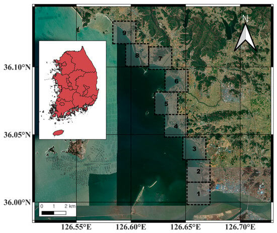
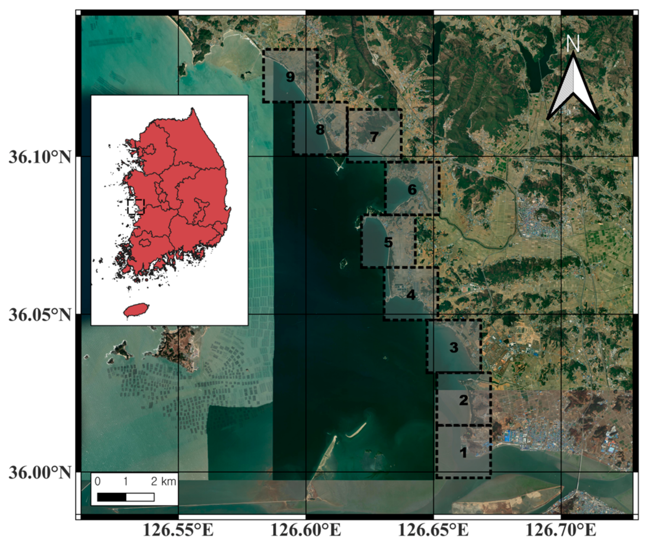
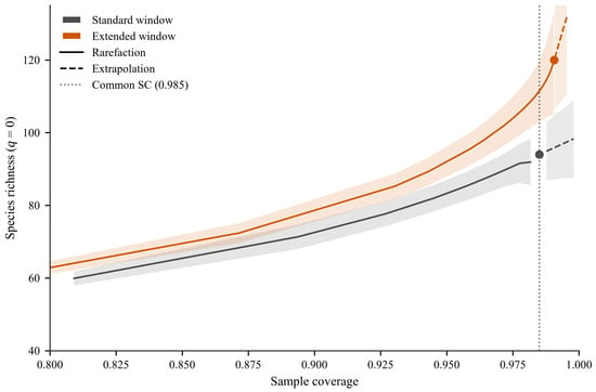
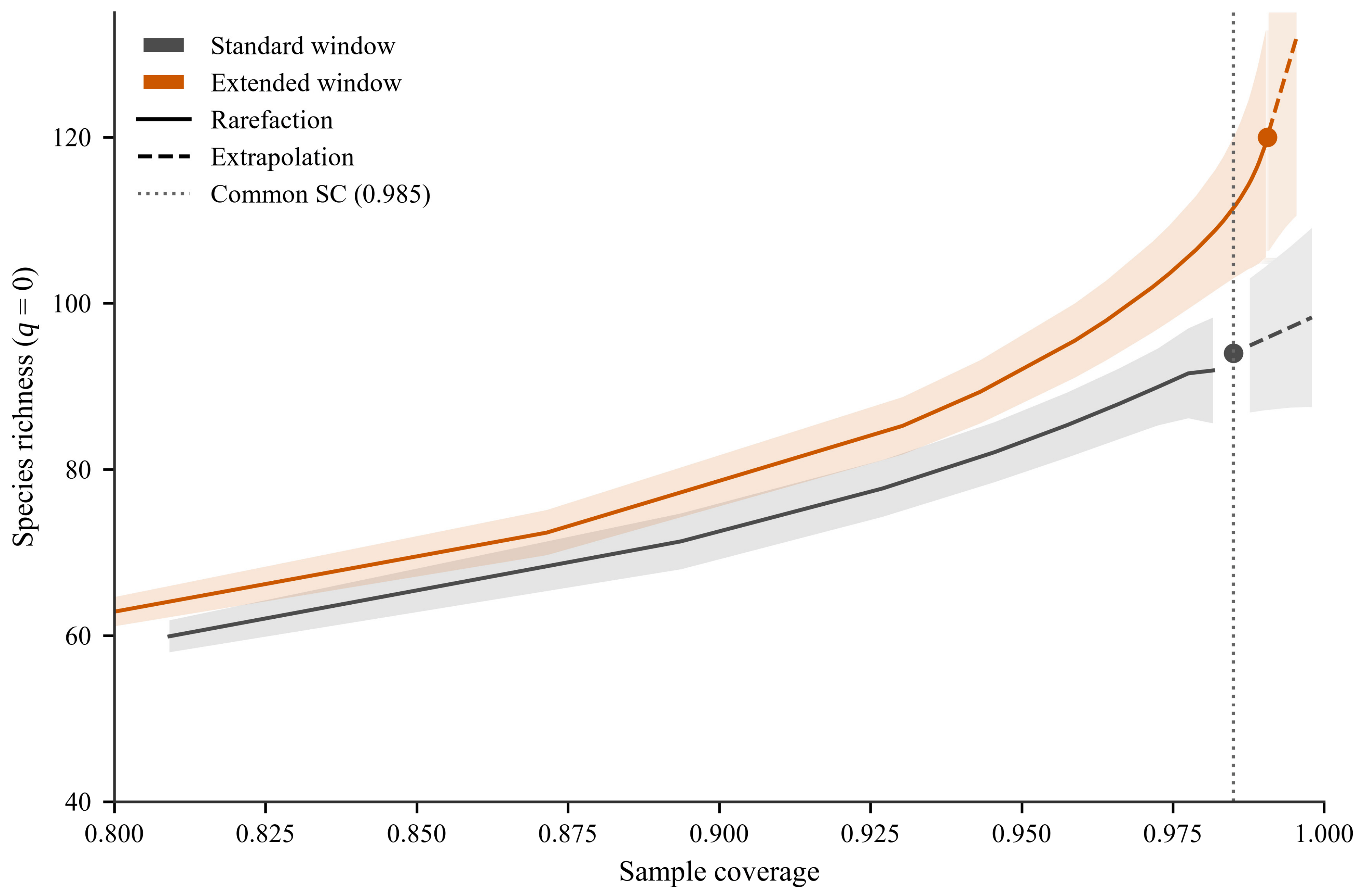
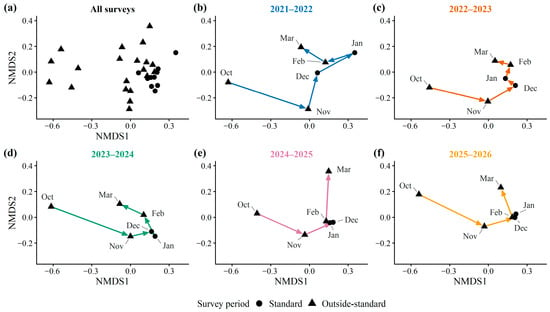
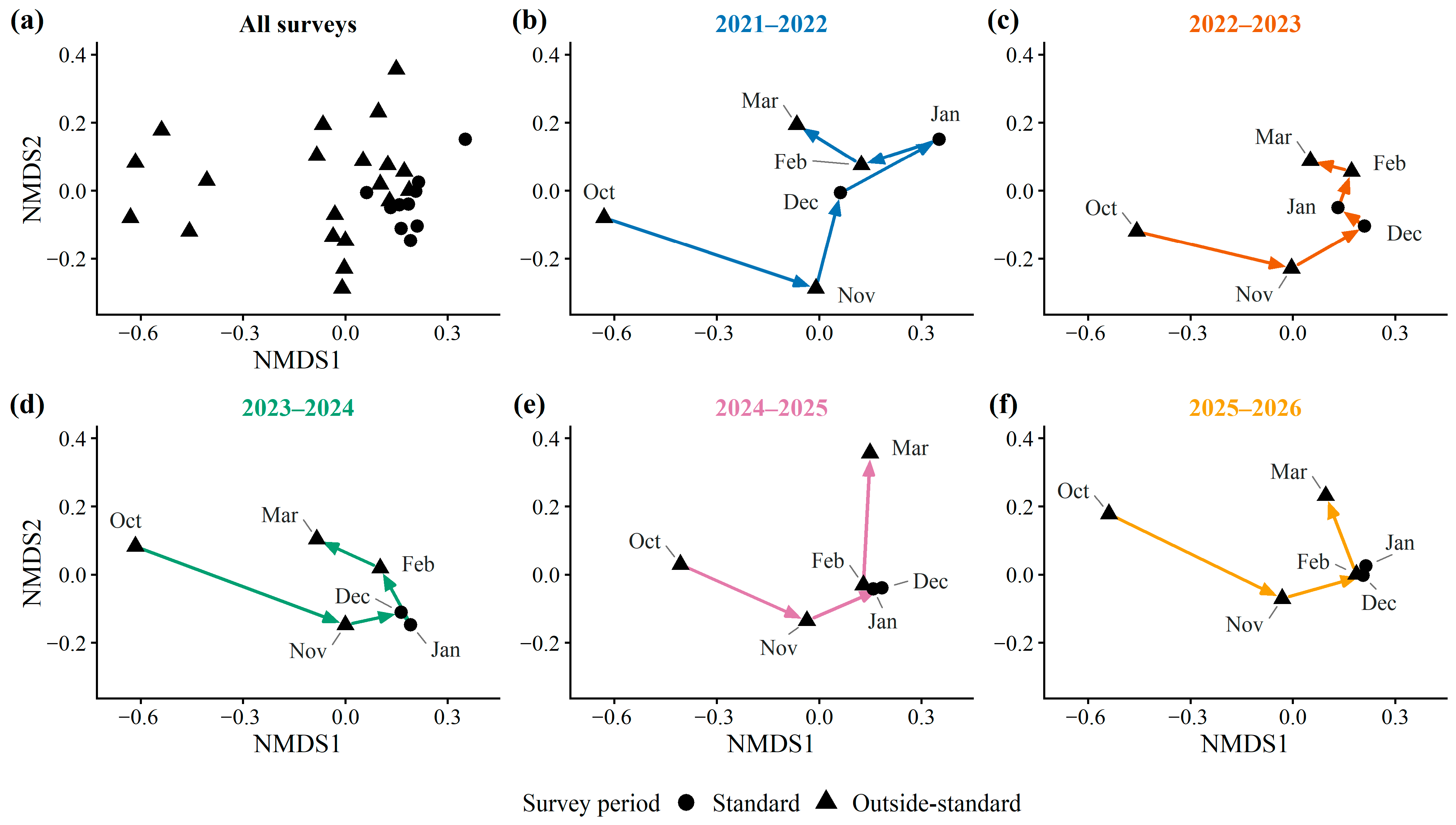
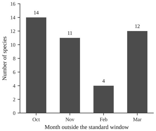
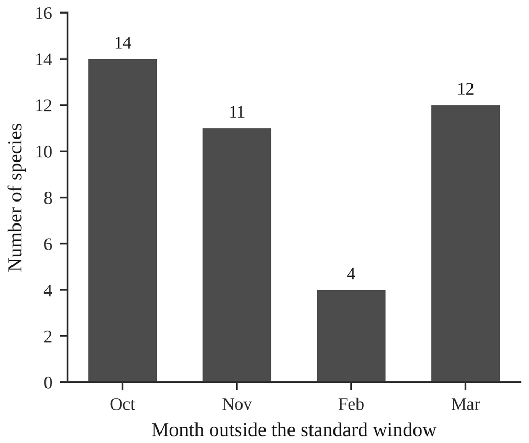
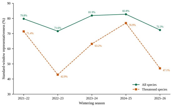
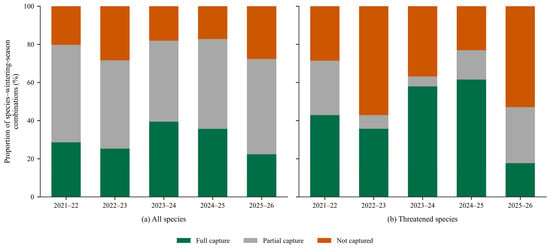
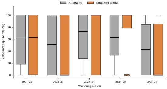
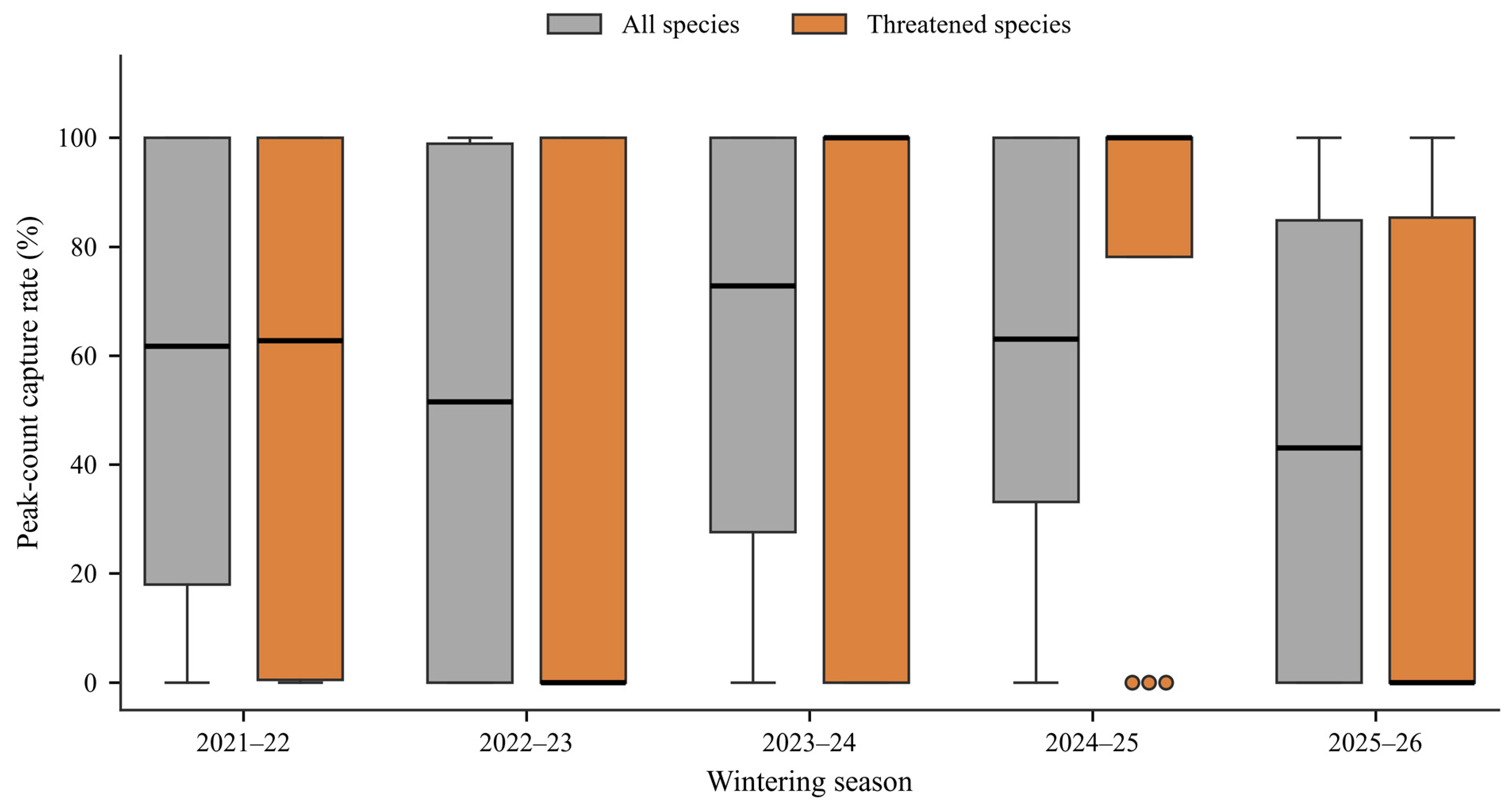

Disclaimer/Publisher’s Note: The statements, opinions and data contained in all publications are solely those of the individual author(s) and contributor(s) and not of MDPI and/or the editor(s). MDPI and/or the editor(s) disclaim responsibility for any injury to people or property resulting from any ideas, methods, instructions or products referred to in the content. |
© 2026 by the authors. Licensee MDPI, Basel, Switzerland. This article is an open access article distributed under the terms and conditions of the Creative Commons Attribution (CC BY) license.