Sampling Bias, Floristic Differentiation, and Conservation Screening in South Korean Limestone-Area Plant Occurrence Records

Abstract

Historical occurrence records combine floristic patterns with uneven survey histories. We analyzed 69,707 vascular-plant records representing 2209 standardized taxa from limestone-bearing areas of South Korea in 10 km × 10 km grids. Observed richness correlated strongly with record count across 129 recorded grids (Spearman ρ = 0.996). Among 66 grids with at least 100 records, expected richness in 100 records had little monotonic association with record count (ρ = 0.021), but closely tracked record-frequency diversity (Hurlbert PIE; ρ = 0.992). Observed and standardized richness ranks shared one top-10 grid. Primary 100-record Sørensen dissimilarity had a median of 0.892 and geographic-distance correlation of 0.352. Standardized geographic and composite PCA environmental-distance coefficients were 0.338 and 0.044 (R² = 0.127), remaining similar after accounting for record counts and source composition. In separate geography-adjusted models, elevation distance was associated with dissimilarity (β = 0.362; exploratory), indicating dependence on environmental-distance definition. Excluding cultivation-flagged taxa preserved dissimilarity ranks (ρ = 0.993). Separate conservation-attribute and alien-occurrence indices identified provisional candidate groups whose membership frequencies depended on resampling cutoffs. These records support descriptive regional comparisons and survey targeting, while recording processes constrain ecological interpretation.

1. Introduction

Limestone landscapes can contain spatially restricted habitats and conservation-important biota while also being exposed to land-use pressures. Studies of Asian karst systems have therefore emphasized the need to document and prioritize biodiversity before habitat loss occurs [1]. Field surveys and synthesis from Korean limestone areas likewise document distinctive floras containing endemic, red-listed, and alien taxa [2]. Regional assessments, however, often rely on records assembled from different agencies, projects, years, and survey purposes rather than on one probability-based sampling design.

Korean limestone habitats include geographically separated outcrops with conservation issues that extend beyond species totals. For example, population-genetic work on the endemic shrub Zabelia tyaihyonii documents the importance of population history and differentiation in limestone forests [3]. Regional occurrence summaries can locate gaps and candidate areas, but they cannot substitute for this population-level evidence or identify limestone preference without a non-limestone comparison.

Presence-only records capture both plant occurrence and observation effort. Accessibility, observer activity, taxonomic interest, and source coverage can bias their spatial and environmental distribution [4,5,6,7,8]. A grid without records is not a confirmed absence, while observed richness tends to increase with record number [9,10,11]. These properties complicate comparisons among limestone grids compiled from different surveys.

Coverage-based rarefaction supports comparisons at similar sample completeness when sampling units are commensurate [12,13,14]. In heterogeneous legacy data, equal record totals do not ensure comparable survey processes, and undersampling can alter dissimilarity in metric-dependent ways [15,16]. We used the conventional Sørensen dissimilarity and its turnover and nestedness-resultant components [17,18], then evaluated the finite-record dependence of an author-defined diagnostic derived from a within-grid resampling reference. This distinction matters when translating recorded beta diversity into conservation screening [19]. Conservation attributes and alien occurrence were evaluated separately because they inform different screening questions [20,21,22,23].

Korean limestone floras and conservation-important taxa have been documented [2], but the combined effects of uneven record accumulation on grid-level richness, compositional differentiation, and conservation screening have not been evaluated across the mapped Korean limestone domain. Assessing these outcomes together can identify where historical records support regional comparison and where field verification is needed.

This study evaluated vascular-plant occurrence records within mapped limestone-bearing areas of South Korea. We asked: (1) How strongly observed richness covaried with record accumulation; (2) what coverage- and fixed-record standardization measured in this database; (3) how record-standardized composition related to geographic and occurrence-associated environmental distance, and how these patterns changed with analytical choices; and (4) how conservation attributes and alien occurrence could identify provisional grids for field verification. The limestone-only design did not test preference relative to non-limestone habitats.

2. Materials and Methods

2.1. Study Area and Plant Occurrence Data

The study covered South Korea. Limestone distribution was delimited with the 2025 KIGAM 1:25,000 geological-map data [24]. Geological units whose lithology names contained ‘limestone’ were selected and rasterized as a binary 100 m limestone layer in EPSG:5186. Plant occurrence records within this mapped distribution were then extracted. The mapped layer was a spatial selection criterion; occurrence within it does not establish that a taxon is a limestone specialist. Maps were prepared using QGIS (version 3.34).

We used plant occurrence data analyzed by Hong et al. (2025) [25]. These data combine observations from several survey programs, including the National Institute of Biological Resources (NIBR), the NIBR biogeographic information service, Korea National Park Service (KNPS), and the second through fifth National Ecosystem Surveys (NIE2nd–NIE5th). Table S1 defines all 13 source categories and summarizes their survey context and observation periods. We used taxon names standardized against the National Species List of South Korea, retaining the taxonomic units distinguished in that list; the integration and name-standardization procedures are described in earlier studies [26,27]. Grids without records were treated as unrecorded, not as confirmed absences.

2.2. Spatial Aggregation and Uneven Record Accumulation

Occurrence records and mapped limestone area were aggregated into 10 km × 10 km grids. Grids containing at least one 100 m limestone raster cell formed the study domain. The 10 km grid was a regional reporting unit and does not imply a homogeneous limestone habitat throughout each grid.

We summarized variation in record accumulation using ranges, medians, source shares, and Gini coefficients. Among grids with records, Spearman correlations compared observed taxon richness with record count, the number of distinct source–year combinations, and mapped limestone area. Source–year combinations counted the distinct data-source and calendar-year combinations with records in each grid. A diagnostic linear model related log(1 + observed richness) to log(1 + record count) and log(1 + limestone area).

2.3. Record Standardization and Richness Sensitivities

To evaluate coverage standardization, each source–year combination formed one grouping within a grid, and each taxon was scored once per grouping. Coverage-based rarefaction was assessed for grids with at least five such groupings [12,13,14], with extrapolation limited to twice the observed number of groupings. We repeated the diagnostic with source–year–coordinate groupings. Neither grouping represents field visits with equal survey effort.

For fixed-record standardization, each database row was one record, and we sampled rows without replacement within each grid. If a grid had N records, of which n_i belonged to taxon i, the probability that taxon i occurred in a sample of m records was 1 − C(N − n_i, m)/C(N, m), where C denotes combinations. Expected richness was the sum of these inclusion probabilities [9,28]; its value at m = 100 is denoted S₁₀₀. Record frequency determined sampling probabilities and was not treated as organism abundance. We compared S₁₀₀ with the proportion of single-record taxa, observed taxa per record, source shares, and Hurlbert’s PIE, calculated as N/(N − 1) × [1 − Σ(n_i/N)²] [29].

We evaluated targets of 25, 50, 100, and 200 records without extrapolation, retaining only grids with at least the target number of records. For each eligible grid and target, 5000 multivariate hypergeometric draws gave the 2.5th and 97.5th percentiles of subsampled richness. The principal analysis used 100 records; threshold sensitivity compared the same 58 grids with at least 200 records. Observed and standardized richness ranks were compared using Spearman correlation, overlap among the ten highest-ranked grids, and absolute rank shifts. Mean ranks were used for correlation and minimum ranks for reported positions. These intervals describe subsampling variation conditional on the observed records, not uncertainty about a grid’s complete flora.

For source sensitivity, we removed each of the 13 source categories in turn and repeated 100-record standardization. Comparisons used grids that remained eligible after removal; richness ranks and conservation-screening percentiles were recalculated on the common eligible grids. Sensitivity results are summarized in Table S2.

For temporal sensitivity, we separately analyzed records from 2006 to 2018 and 2015–2024, reassessing eligibility at 100 records in each window. The windows overlap and were used as alternative restrictions on the pooled data, not independent tests of ecological change. Richness ranks and top-ten overlap were compared with the corresponding full-period results and after reranking on common eligible grids; compositional comparisons used 1000 draws.

In an additional sensitivity, taxa carrying a cultivation-status flag were excluded and richness and Sørensen dissimilarity were recalculated with 1000 draws. This taxon-level flag does not establish that an individual record represents a planted plant.

2.4. Between-Grid Composition and Within-Grid Variation

Between-grid composition was compared using taxon presence and Sørensen dissimilarity, partitioned into Simpson turnover and nestedness-resultant components following Baselga [17,18]. The principal analysis included 66 grids with at least 100 records. We drew 100 records without replacement per grid in 1000 replicates and used the mean pairwise Sørensen dissimilarity as the primary response. Threshold sensitivity used the same 58 grids with at least 200 records, drawing 25, 50, 100, or 200 records in 500 replicates per threshold.

To assess variation caused by resampling within a grid, each replicate r included two independent 100-record draws per grid. B_ij^(r) denotes dissimilarity between the first samples from grids i and j, and W_i^(r) denotes dissimilarity between the two samples from grid i. The pair-specific within-grid reference was the arithmetic mean of the two within-grid dissimilarities, giving equal weight to references based on the same sample size and ensuring symmetry when the grid labels were exchanged:

$$W_{\mathit{ij}}^{\left(r\right)}={\displaystyle \frac{W_i^{\left(r\right)}+W_j^{\left(r\right)}}{2}}$$

(1)

Although each sample was drawn without replacement, independently drawn samples could share records. For a pool of N records and sample size m, their expected record overlap is m²/N; thus, the within-grid reference can depend on pool size. Across 1000 replicates, mean between-grid dissimilarity and mean pair-specific reference were denoted ${\overline{B}}_{\mathit{ij}}$ and ${\overline{W}}_{\mathit{ij}}$, respectively. We defined the following secondary diagnostic:

$$D_{\mathit{ij}}={\displaystyle \frac{{\overline{B}}_{\mathit{ij}}-{\overline{W}}_{\mathit{ij}}}{1-{\overline{W}}_{\mathit{ij}}}}$$

(2)

D is zero when the two means coincide, may be negative, becomes sensitive to small changes as ${\overline{W}}_{\mathit{ij}}$ approaches one and the denominator approaches zero, and is undefined when ${\overline{W}}_{\mathit{ij}}$ = 1. It was not interpreted as a correction for incomplete detection or survey bias. For sensitivity, we also compared raw-presence Sørensen dissimilarity and the unscaled difference ${\overline{B}}_{\mathit{ij}}$ − ${\overline{W}}_{\mathit{ij}}$.

We examined the dependence of grid-level W on record count and drew two disjoint 100-record subsets from 200 distinct records within each of the same 58 eligible grids (1000 replicates). Under an identical-assemblage null, two grids shared the same 500 equiprobable taxa. Independent record pools of N = 100, 200, 500, or 2000 were generated 100 times per condition and resampled 100 times per dataset. Overlapping independent draws were compared with disjoint draws where N ≥ 200 to assess dependence of D on pool size and sampling design.

2.5. Geographic and Environmental Relationships

Geographic distance was the Euclidean distance in kilometers between grid-level mean projected occurrence coordinates (EPSG:5186). Its association with compositional dissimilarity was assessed by a Spearman Mantel test [30] with 999 simultaneous row-and-column permutations of grid labels and a two-sided test.

Environmental values attached to the integrated occurrence data were used [26,27]. Elevation, slope, and aspect originated from the National Geographic Information Institute digital elevation model (2024; native resolution 30 m), with elevation represented by the 1 km values used in the source data [31]. Mean temperature, precipitation, wind speed, humidity, and solar radiation originated from Korea Meteorological Administration data [32]. For each grid, elevation, slope, and the five meteorological variables were summarized as medians across occurrence rows. Aspect was transformed to eastness (sin aspect) and northness (cos aspect), then averaged. Missing values were omitted on a variable-by-variable basis, and flat-cell aspect codes were excluded from directional means. Repeated records at the same location received repeated weight, so these summaries describe recorded locations rather than all limestone habitat within a grid.

Nine environmental variables were standardized and reduced by PCA, retaining the fewest axes explaining at least 80% of the variance. Euclidean environmental distance was computed from retained PC scores on their original, unwhitened variance scales. Multiple regression on distance matrices [33] related the principal 100-record Sørensen response to log(1 + geographic distance) and PCA environmental distance. Standardized coefficients and pairwise-distance R² were evaluated using 999 simultaneous row-and-column permutations of response grid labels; these unrestricted permutations do not preserve spatial autocorrelation and were interpreted as exploratory [30,34]. We varied PC retention, excluded one grid at a time, and tested each of the nine individual environmental distances jointly with geographic distance, applying Benjamini–Hochberg adjustment across the nine tests. An equal-coordinate-weight analysis assessed the effect of repeated occurrence locations. Additional fits included pairwise mean and absolute difference in log record count, followed by the Bray–Curtis distance between the grids’ proportions of records from the 13 sources. The same covariates were added to the geography–elevation model. Comparisons used the same 66 grids and 2145 pairs.

2.6. Conservation and Alien-Taxon Screening

To compare conservation-related and alien-taxon occurrences among grids, we used the taxon attributes in the integrated data [26,27]. The conservation components were Korean endangered wildlife Class I or II (P), Korean endemic taxa (E), and taxa classified as Critically Endangered, Endangered, or Vulnerable in the national Red List (R). P is a legal designation under Article 2 and Appendix 1 of the Enforcement Rule of the Wildlife Protection and Management Act [35]; R is a scientific extinction-risk assessment [36]. These attributes can overlap but have distinct meanings.

Alien taxa (A) are taxa introduced outside their native range through human activity [37] and were operationally identified by the alien-status flag in the source data [26,27]. The flag does not indicate whether an occurrence was invasive or caused ecological harm.

We calculated the expected number of distinct P, E, R, and A taxa in a 100-record sample per grid. For each component across the 66 eligible grids, percentile ranks were computed as (rank − 1)/(n − 1), with mean ranks for ties and n denoting grid count. CPI-R was 100 times the equally weighted mean of the P, E, and R percentile ranks; the alien-occurrence percentile was 100 times the A rank. A raw CPI-R for comparison used observed rather than 100-record expected component counts. Alien taxa were screened separately and were not subtracted from CPI-R.

The 75th percentiles of CPI-R and alien occurrence defined upper groups, including values equal to either cutoff. Grids were classified as joint-high, conservation-attribute only, alien-occurrence only, or other screened. We assessed stability with 1000 independent 100-record draws per grid, recalculating component ranks and scores in each replicate. We report conditional medians and 2.5th–97.5th percentile intervals and distinguish membership frequencies using replicate-specific cutoffs from those using fixed point-estimate cutoffs; neither is a probability of true conservation priority. Threshold sensitivity compared scores and upper-group overlap on the same 58 grids with at least 200 records. We also omitted P, E, and R in turn and compared CPI-R ranks and upper-quartile membership with the three-component index. Grid-specific components and screening results are given in Table S3. Statistical analyses were performed using Python (version 3.11).

3. Results

3.1. Data Coverage and Record Accumulation

The dataset contained 69,707 occurrence records and 2209 standardized taxa from 13 assigned source categories. Dated records spanned 1969–2024, and eight records had unknown years.

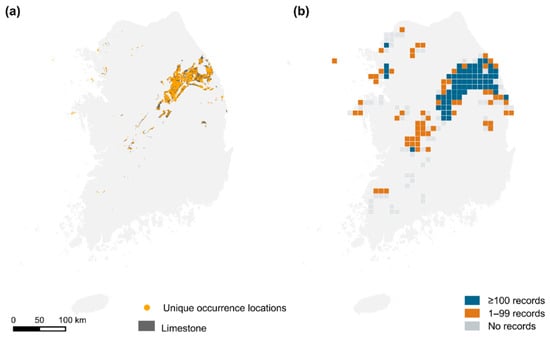
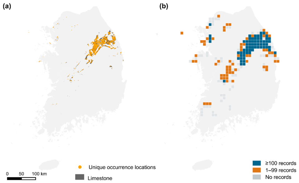
The limestone raster contained 2976.64 km² of mapped limestone in 194 grids. Of these, 66 grids contained at least 100 records and were included in the principal analysis, 63 contained 1–99 records and were ineligible for the 100-record analysis, and 65 contained no occurrence records (Figure 1). The 66 analyzed grids represented 34.0% of all limestone-bearing grids but contained 2648.86 km², or 89.0%, of the mapped limestone area. Analytical eligibility indicates the availability of occurrence records and does not indicate ecological or conservation value.

Figure 1. Limestone distribution and spatial coverage of occurrence data. (a) Mapped limestone raster cells and unique occurrence locations. (b) Analytical status of the 194 limestone-bearing 10 km × 10 km grids: analyzed grids with at least 100 records (n = 66), ineligible grids with 1–99 records (n = 63), and unrecorded grids with no occurrence records (n = 65). The categories indicate occurrence-data availability and eligibility for the principal 100-record analysis, not ecological or conservation value.

Temporal coverage differed among sources (Table S1). Median observation years were 2014 for NIBR and NIBR biogeographic information service, 2016 for KNPS, and 1998, 2011, 2018 and 2023 for NIE2nd, NIE3rd, NIE4th and NIE5th, respectively.

Among the 129 record-bearing grids, record counts ranged from 1 to 4079 (median = 123), observed richness ranged from 1 to 985 taxa (median = 91), and source–year combination counts ranged from 1 to 50 (median = 10). Fourteen grids contained just one observed taxon: 12 had one occurrence record and two had two records of the same standardized taxon. All 14 had fewer than 100 records and were excluded from the principal analysis; observed richness among the 66 eligible grids ranged from 66 to 985 taxa. The minimum of one reflects sparse records rather than the complete flora of a 10 km grid. Grid-record Gini coefficients were 0.698 for record-bearing grids and 0.799 for all limestone-bearing grids. The Gini coefficient for record counts across source–year combinations was 0.745.

NIBR biogeographic information service contributed 20,996 records (30.1%), NIBR 16,359 (23.5%), NIE5th 9621 (13.8%), NIE4th 6586 (9.4%), and NIE3rd 5112 (7.3%). Contributions from all 13 assigned source categories are shown in Table S1. Percentages use all 69,707 records as their denominator.

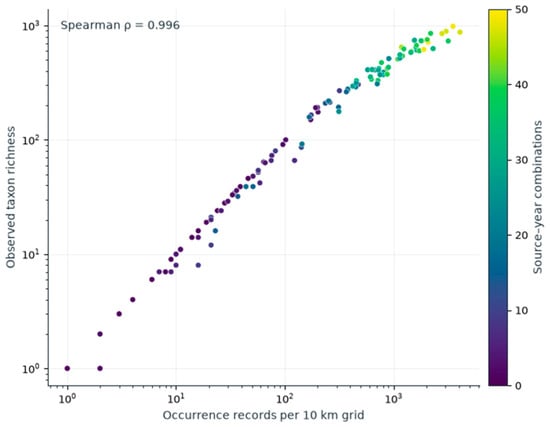
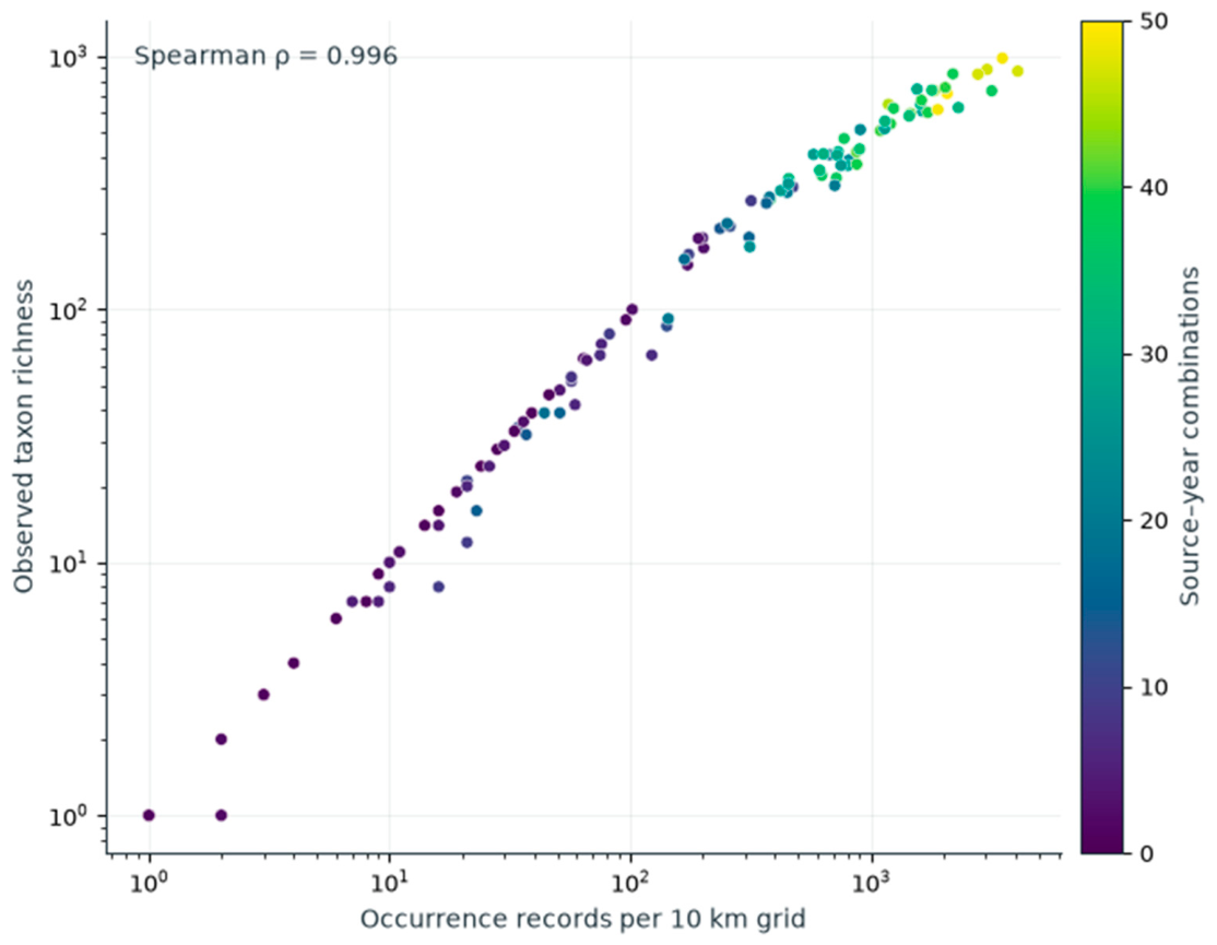
Observed richness had Spearman correlations of ρ = 0.996 with record count, ρ = 0.900 with source–year combination count, and ρ = 0.844 with limestone area (all p < 0.001; Figure 2). The diagnostic log-linear model had adjusted R² = 0.987. Coefficients were 0.901 for log(1 + record count) (p < 0.001) and −0.084 for log(1 + limestone area) (p = 0.002).

Figure 2. Observed taxon richness and occurrence-record count in 129 record-bearing 10 km grids. Both axes use logarithmic scales and include all 69,707 records. Color denotes source–year combination count. Twelve grids with one occurrence record and one observed taxon overlap at (1,1).

3.2. Coverage-Standardization Applicability

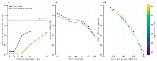
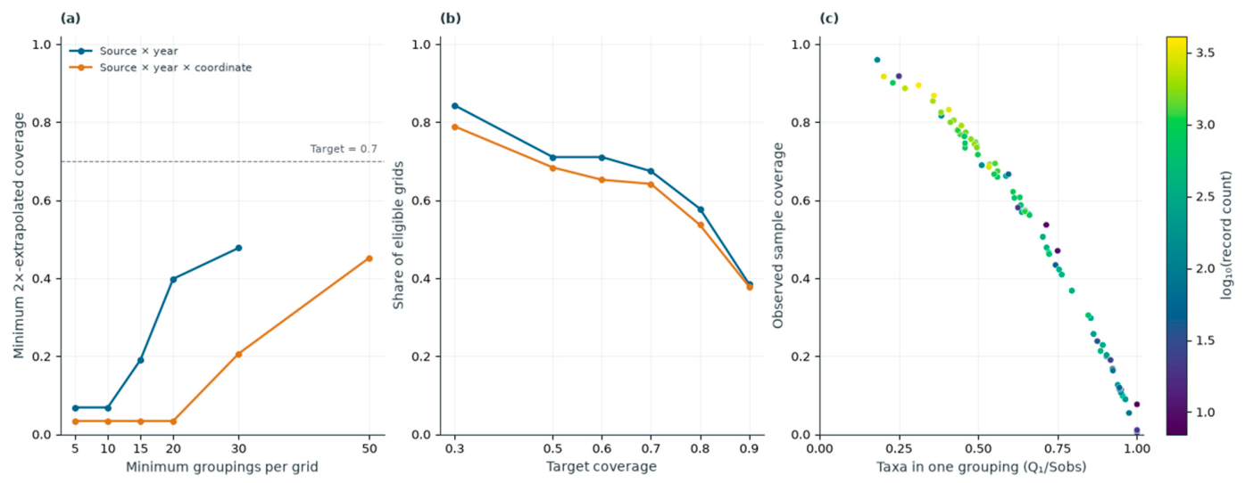
Among 83 grids containing at least five source–year groupings, observed coverage ranged from 0.005 to 0.960 (median = 0.588), and twofold-extrapolated coverage ranged from 0.069 to 1.000 (median = 0.841). The minimum is an extreme-grid constraint rather than typical completeness.

At target coverages of 0.5, 0.7 and 0.8, the source–year definition retained 59, 56 and 48 of 83 grids, respectively. The source × year × coordinate definition retained 65, 61 and 51 of 95 grids, respectively (Figure 3). These percentages use proxy-specific eligible sets. Relative to all 129 recorded grids, source–year coverage 0.7 retained 56 grids (43.4%), whereas the 100-record threshold retained 66 (51.2%); retention alone does not establish comparable sampling units.

Figure 3. Applicability of incidence-based coverage standardization using all 69,707 records. (a) Minimum twofold-extrapolated coverage by the minimum number of groupings per grid. (b) Share of eligible grids retained at fixed coverage targets. (c) Observed coverage versus the proportion of taxa recorded in one source–year grouping (Q1/Sobs); color indicates log10-transformed record count. The one-grid source–year result at 50 groupings is omitted in (a); initial eligibility was 83 and 95 grids. Panel (c) is a descriptive diagnostic mathematically coupled to the coverage estimator, not an independent validation.

3.3. Record-Standardized Richness

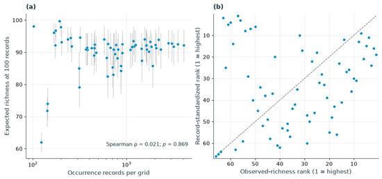
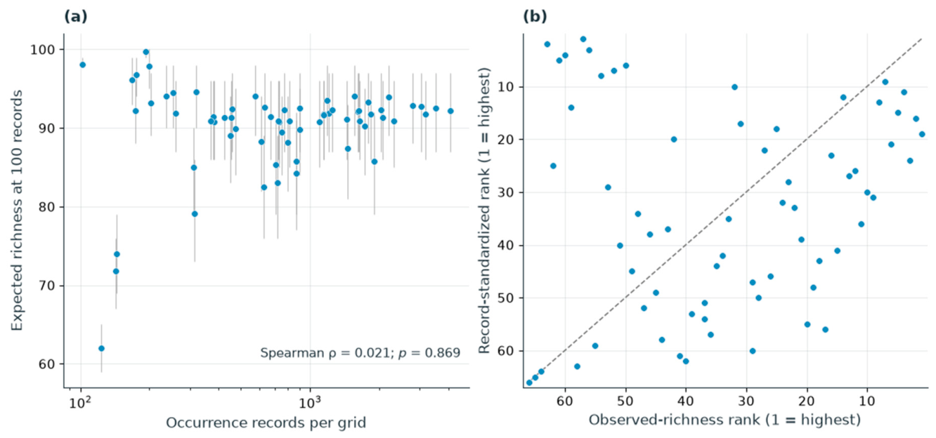
Record thresholds of 25, 50, 100, and 200 retained 88, 78, 66, and 58 grids, respectively (Table S2.1). At 100 records, observed richness had ρ = 0.978 with total record count, whereas standardized richness had ρ = 0.021 (p = 0.869). Correlations of standardized richness with limestone area and source–year combination count were 0.015 and −0.123, respectively (p = 0.904 and p = 0.325).

At 100 records, observed and standardized richness ranks had ρ = 0.146 (p = 0.243), their top-10 overlap was one grid, and the median absolute rank change was 14.5 positions (maximum = 61; Figure 4). Pairwise correlations among standardized ranks at the four thresholds ranged from 0.986 to 0.999 on the common 58-grid set.

Figure 4. Record-standardized richness across 66 grids with at least 100 records. (a) Expected richness in 100 records versus total record count; vertical lines indicate 95% random-subsampling intervals. (b) Observed versus standardized richness ranks (1 = highest); the dashed line indicates identical ranks. The top-10 lists share one grid. Intervals describe draws from the observed record pool.

Expected richness in 100 records had median 91.56 (range 62.00–99.73), with 54 of 66 grids concentrated above 85 and at or below 95; five exceeded 95. Its correlations with record-frequency PIE, singleton fraction, and observed taxa per record were 0.992, 0.317, and 0.270, respectively (Table S2.2). Associations with source proportions included NIBR (ρ = −0.441), NIBR biogeographic information service (−0.311), and NIE5th (0.279). The eight highest-ranked grids had only 102–318 records and observed-richness ranks of 50–63.

3.4. Source, Temporal, and Cultivation Sensitivity Analyses

Removing each of the 13 source categories left 62–66 grids eligible at the 100-record threshold. Correlations between all-source and source-removal standardized-richness ranks ranged from 0.837 to 1.000 on the common eligible sets (Table S2.3). The lowest correlations followed removal of NIBR (ρ = 0.837; 63 grids) and NIBR biogeographic information service (ρ = 0.839; 63 grids).

Source-removal comparisons shared 7–10 of the ten highest-ranked grids with their reference, and maximum absolute rank shifts ranged from 1 to 44 positions. Removing NIBR biogeographic information service shared seven top-ranked grids, while removing NIE5th produced the largest rank shift.

The 2006–2018 and 2015–2024 analyses retained 59 and 58 grids at the 100-record threshold, respectively. Within these period-specific grid sets, correlations between observed richness and record count remained high (ρ = 0.967 and 0.977, respectively), whereas correlations between 100-record-standardized richness and record count were ρ = 0.023 and 0.077. Standardized-richness rank correlations with the corresponding full-period values were ρ = 0.842 for 2006–2018 and ρ = 0.781 for 2015–2024. In each window, only seven of the full-period top-10 grids remained eligible, and six were retained in the period-specific top 10. Reranking both datasets on common eligible grids gave seven shared top-10 grids (Table S2.3).

Median primary 100-record Sørensen dissimilarity was 0.888 for 2006–2018 and 0.887 for 2015–2024. Pairwise correlations with full-period dissimilarities on shared grid pairs were 0.909 and 0.813; corresponding geographic-distance correlations were 0.343 and 0.389.

Excluding cultivation-flagged taxa retained 67,477 records and 2002 taxa. All 66 principal grids remained eligible; standardized richness ranks correlated with the primary analysis at ρ = 0.996, and the Sørensen pair correlation was ρ = 0.993.

3.5. Beta-Diversity Patterns

Raw pairwise Sørensen dissimilarity among 66 grids had a median of 0.638, with median turnover and nestedness-resultant components of 0.420 and 0.148. At 100 records, the corresponding medians were 0.892, 0.888, and 0.002. The mean turnover component divided by mean total standardized Sørensen dissimilarity was 99.5%. Raw and standardized total-dissimilarity ranks had ρ = 0.366 (p < 0.001). Component medians are marginal summaries: turnover plus nestedness-resultant dissimilarity equaled total Sørensen dissimilarity for every grid pair, but the separately calculated marginal medians were not required to sum.

The within-grid reference correlated strongly with record count (ρ = 0.969). On the same 58 grids with ≥200 records, preventing record overlap between the two 100-record samples changed the reference-derived D median from 0.606 to 0.322 and its geographic correlation from 0.493 to 0.378. Under the identical-assemblage null, overlapping-draw median D declined from 0.816 at N = 100 to 0.171 at N = 2000. In contrast, disjoint-draw medians were 0.010, −0.006, and approximately zero at N = 200, 500, and 2000, respectively. Disjoint sampling reduced the artifact under this uniform-frequency null; both D variants remained secondary diagnostics (Table S2.4).

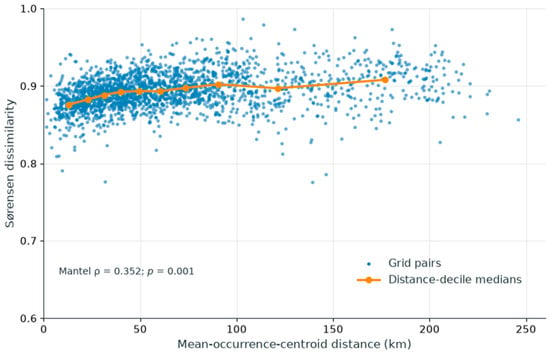
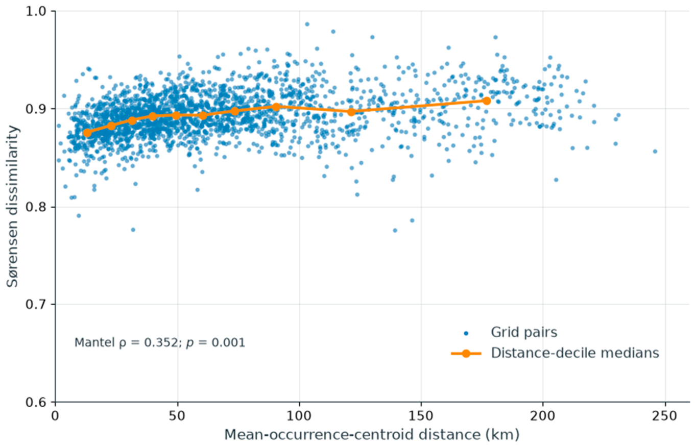
Mean occurrence centroids were 2.94 km from cell centers on average (maximum 6.18 km). The primary 100-record Sørensen response correlated with geographic distance at ρ = 0.352 (p = 0.001, the minimum attainable value for 999 permutations; Figure 5). The turnover and nestedness-resultant correlations were 0.348 (p = 0.001, minimum attainable) and −0.044 (p = 0.519), respectively. On the common 58-grid threshold set, geographic correlations for conventional Sørensen ranged from 0.382 to 0.408 across 25–200 records (Table S2.1).

Figure 5. Primary 100-record Sørensen dissimilarity versus distance among 2145 pairs of 66 grids. Blue points denote grid pairs; orange points and connecting lines denote geographic-distance-decile medians. Distance is between mean occurrence coordinates. The y-axis spans 0.6–1.0; all grid pairs are displayed. The annotation reports the descriptive Mantel correlation and unrestricted permutation p value; these are not spatially controlled tests of ecological mechanisms.

3.6. Geographic and Environmental Associations

Six PCA axes explained 86.8% of variance in the occurrence-associated environmental summaries. Environmental and geographic distances had a Mantel correlation of ρ = 0.406 (p = 0.001).

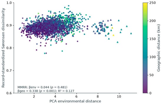
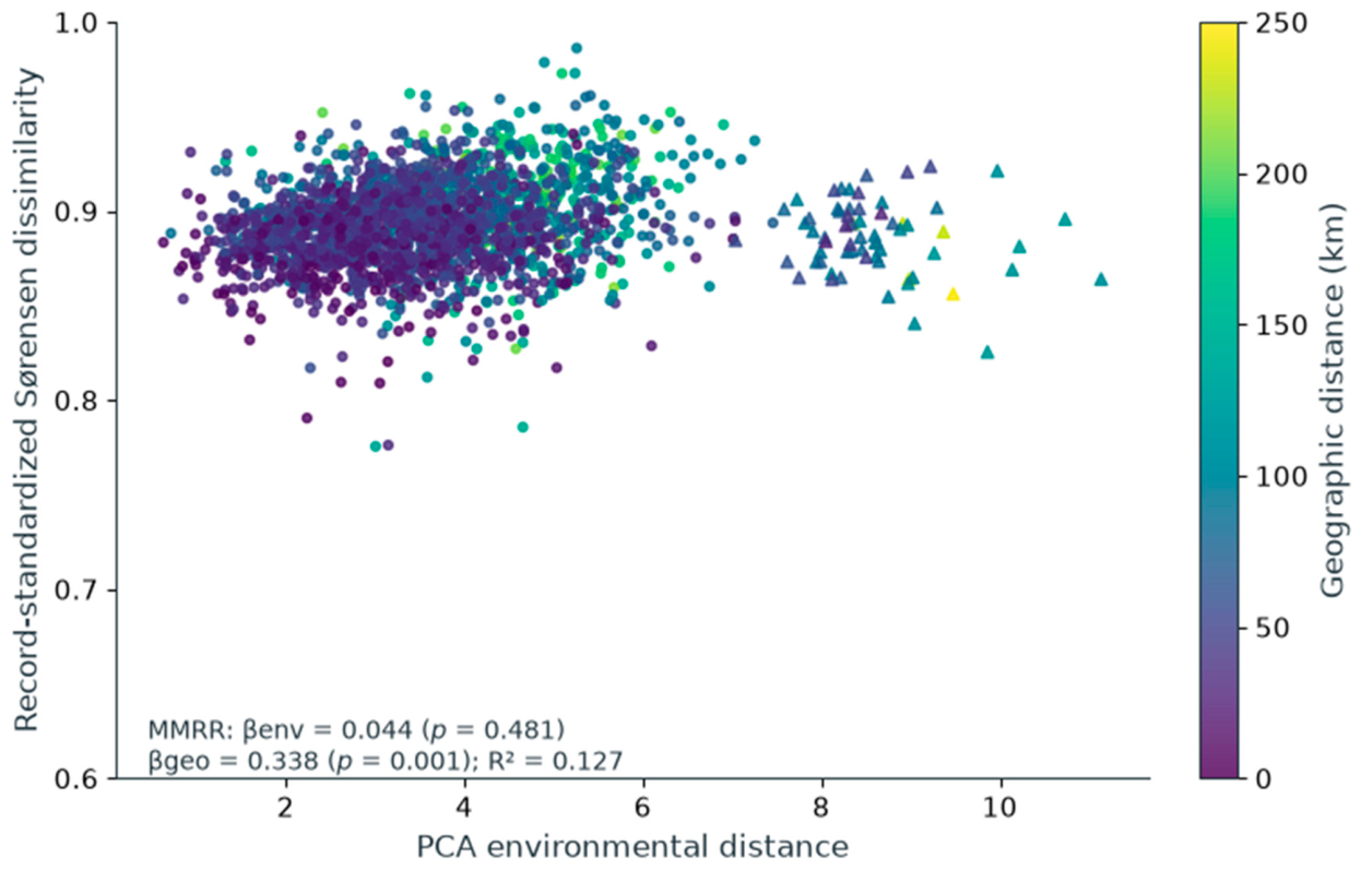
For the primary 100-record Sørensen dissimilarity, standardized coefficients were 0.338 for geographic distance (p = 0.001) and 0.044 for environmental distance (p = 0.481), with R² = 0.127. Thus, composite PCA environmental distance added little explanatory information to this descriptive distance model (Table 1; Figure 6).

Table 1. Descriptive distance-matrix regressions for primary and sensitivity responses in 66 grids.

Response/Model	Geography β	Environment β (PCA or Elevation)	R2 (%)
100-record Sørensen	0.338	0.044	12.7
+ Record counts	0.362	0.075	14.1
+ Record counts and sources	0.360	0.074	14.2
100-record: geography + elevation	0.277	0.362	25.1
+ Record counts and sources (elevation)	0.282	0.365	26.0
Raw presence	0.343	0.267	25.7
Reference-derived D	0.368	0.277	28.9
Between−within	0.250	0.268	18.4

β values are standardized regression coefficients. Environment is PCA distance except in the elevation models. Record-count covariates are the pairwise mean and absolute difference in log N; source composition is the Bray–Curtis distance among 13 source proportions (Table S2.6). Reference-derived D uses overlapping draws (Table S2.4). Raw presence is sensitive to record count and inventory completeness. R² describes pairwise dissimilarity variation. Unrestricted permutation tests reported in the text do not control spatial autocorrelation.

Figure 6. Primary 100-record Sørensen dissimilarity versus PCA environmental distance among 2145 pairs of 66 grids. Symbol color denotes geographic distance. The triangles identify all 65 pairs including G10_E041_N048; 54 of these have environmental distance ≥8. The y-axis spans 0.6–1.0. The annotation reports standardized regression coefficients, unrestricted permutation p values, and R² of pairwise dissimilarities. Environmental attributes describe occurrence locations; the model is exploratory. Grid locations and details are provided in Table S3.

Environmental coefficients ranged from 0.038 to 0.064 across PCA-retention settings and from 0.018 to 0.135 across leave-one-grid-out fits. Individual-variable models, each adjusted for geographic distance, identified elevation (β = 0.362; BH-adjusted p = 0.009) and slope (β = 0.160; adjusted p = 0.018), interpreted as exploratory. The geography–elevation model had geographic β = 0.277 and R² = 0.251 (Table 1; Table S2.5). All 54 pairs with environmental distance ≥8 included G10_E041_N048; the leave-one-grid-out results quantify this dependence.

Adding mean and absolute difference in log record count gave geographic and PCA environmental coefficients of 0.362 and 0.075 (R² = 0.141). Adding source-composition distance gave coefficients of 0.360, 0.074, and 0.023 for geography, PCA environment, and source composition, respectively; the increment was ΔR² < 0.001. In the separate elevation model with both record-count covariates and source composition, elevation β remained 0.365 (geographic β = 0.282; R² = 0.260; Table 1; Table S2.6). Equal weighting of stored coordinates gave geographic and PCA environmental coefficients of 0.330 and 0.065. The reference-derived D environmental coefficient changed from 0.277 to 0.082 after adding record-count covariates. These are descriptive coefficient comparisons, not spatially controlled significance tests.

3.7. Conservation Attributes and Alien-Species Occurrence

Conservation screening was restricted to the 66 grids containing at least 100 occurrence records. The remaining 63 recorded but ineligible grids and 65 unrecorded grids were not assigned conservation or alien-occurrence screening values. The 66-grid analysis set included 18 protected, 122 endemic, 40 CR–EN–VU, and 164 alien taxa. Grid coordinates, record counts, observation years, and index components are listed in Table S3.

Correlations between raw and 100-record-standardized grid ranks were ρ = 0.901 for CPI-R and ρ = 0.583 for the alien-species occurrence percentile.

Expected P, E, and R counts were zero in 29, 2, and 23 grids, respectively. Across resamples, the median numbers of zero-count grids were 42, 8, and 41. These tied component ranks affected the conditional score distributions.

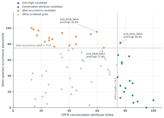
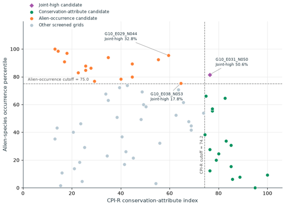
Point-estimate cutoffs of CPI-R = 74.2 and alien-occurrence percentile = 75.0 produced one joint-high candidate, 16 conservation-attribute candidates, 16 alien-occurrence candidates, and 33 other screened grids (Figure 7). For G10_E031_N050, CPI-R was 76.4, its resampling median was 75.5 (95% interval 58.7–91.5), and joint-high frequency was 50.6% with recalculated cutoffs or 24.9% with fixed cutoffs. For G10_E029_N044, CPI-R was 59.5, its resampling median was 61.9 (49.5–71.5), and the corresponding frequencies were 32.8% and 0.4%. For the third labeled grid, G10_E038_N053, joint-high frequencies were 17.8% and 6.8% with recalculated and fixed cutoffs, respectively. The resampled CPI-R cutoff itself had median 66.3 (2.5–97.5% range 61.4–71.5), explaining why the two classification frequencies differ (Table S3).

Figure 7. Relationship between the rank-based conservation-attribute index (CPI-R), calculated from P, E, and R, and the alien-species occurrence percentile among the 66 grids retained at the 100-record threshold. The dashed lines indicate the upper-quartile cutoffs (CPI-R = 74.2; alien-species occurrence percentile = 75.0), and the colors denote point-estimate screening groups. Labels report joint-high frequencies from 1000 replicates with percentile ranks and quartile cutoffs recalculated each time. These relative membership frequencies should not be compared directly with fixed-cutoff exceedance frequencies in Table S3. Grid locations and details are provided in Table S3.

Across the 25–200-record thresholds on the same 58 grids, minimum rank correlations were 0.993 for CPI-R and 0.997 for the alien-species occurrence percentile (Table S2.1). The minimum CPI-R correlation after omission of one of the three components was 0.926. Using the all-source reference and common eligible grid sets, source-removal correlations ranged from 0.921 to 1.000 for CPI-R and from 0.910 to 1.000 for alien-species occurrence (Table S2.3).

4. Discussion

4.1. Record Accumulation and Richness Standardization

Raw richness strongly tracked record accumulation, but the near-zero S₁₀₀–record-count correlation does not validate removal of survey bias. S₁₀₀ closely tracked record-frequency PIE (ρ = 0.992), and high values occurred where most records represented different taxa. Because expected richness in two records equals 1 + PIE [29], these quantities are mathematically related; their strong association is a frequency-distribution diagnostic, not independent validation of standardization or evidence that entire rarefaction curves never cross. Checklist-like accumulation can therefore yield high fixed-record richness even in poorly recorded grids. This is expected richness conditional on an empirical record pool, not an estimate of complete grid richness or pure ecological evenness [9,29]. Upper-end compression also limits interpretation of small rank differences.

Coverage standardization requires interpretable, comparable sampling units [12,13,14]. Neither source–year nor source–year–coordinate groupings established equal survey effort or a consistent checklist process. This non-comparability is the main reason for treating coverage as an applicability diagnostic; retention rates and extreme minimum coverage are secondary considerations. Fixed-record sampling provides a transparent comparison of stored records but cannot correct site selection, taxonomic targeting, or repeated reporting.

Standardized richness ranks were highly consistent across record thresholds, while source-removal correlations ranged from 0.837 to 1.000 and individual grids could move by as many as 44 positions. Source composition therefore remains relevant to individual grid rankings. Rank stability within retained grids and geographic coverage are separate properties of the analysis.

4.2. Compositional Differentiation and Geographic Distance

Primary record-standardized Sørensen dissimilarity increased with geographic distance, and the relationship persisted after excluding cultivation-flagged taxa. Adding record-count and source-composition distances changed the geographic coefficient little. Thus, differences in measured source proportions did not explain the geographic association, although source categories do not identify survey teams, routes, or every reporting practice. The within-grid reference depended strongly on the size of the finite record pool. Disjoint sampling produced near-zero D under the identical, uniform-frequency null; that restricted result does not establish correction under unequal frequencies or heterogeneous detection. Conventional Sørensen therefore remained the primary response, with D used only as a diagnostic.

Turnover comprised nearly all standardized Sørensen dissimilarity under the Baselga partition [15,17,18]. This value describes the algebraic structure of equal-record species lists, in which unmatched species counts were generally balanced between grids. It is not an estimate that the same percentage of ecological change was caused by species replacement. Equalized record totals, incomplete species detection, and pooled survey years all influence the partition [19].

The need for field interpretation is illustrated by Zabelia tyaihyonii: genetic differentiation within a limestone-associated species addresses population processes that pooled grid lists do not measure [3]. The present geographic signal should therefore guide geographically distributed field sampling rather than be attributed directly to dispersal limitation or limestone-driven filtering.

4.3. Geographic and Environmental Associations

The primary distance model showed a positive geographic relationship and a small coefficient for composite PCA environmental distance. In contrast, geography-adjusted elevation distance was associated with dissimilarity, and its coefficient remained similar after accounting for record counts and source composition. The result therefore depends on the environmental-distance definition and does not support a general conclusion that environmental associations are weak. Stronger environmental coefficients in the reference-derived diagnostic and raw-presence response demonstrate method dependence rather than a general environmental effect. Moreover, unrestricted grid-label permutations do not retain spatial autocorrelation, so the reported p values cannot isolate environmental filtering from spatial and recording processes [30,34].

Record-weighted environmental summaries can reflect survey placement and repeated coordinates [38]; giving unique stored coordinates equal weight did not produce a large environmental coefficient. The exploratory elevation and slope associations can reflect topographic habitat differences or preferential survey access along roads and valleys. Survey routes were unavailable, so these alternatives cannot be separated. Independent environmental layers covering the limestone domain and standardized field observations are needed for ecological attribution.

4.4. Conservation-Attribute and Alien-Occurrence Screening

CPI-R and the alien-species occurrence percentile were retained as separate axes because conservation attributes and alien occurrence represent different decision dimensions [20,21,22,23]. The alien axis measures the expected number of distinct alien taxa in a fixed number of records; it does not measure abundance, ecological impact, spread rate, or control feasibility [20,21].

The screening groups are provisional. Rare-species targeting directly affects protected and Red List records, while large blocks of zero or small integer component counts generate tied ranks. Consequently, ranking expected counts and ranking each resample need not produce the same classification. Recalculated-cutoff frequencies express relative standing within each draw, whereas fixed-cutoff frequencies describe a different threshold question. Tied integer component counts alter both the score distribution and recalculated cutoffs; both frequencies are conditional on their respective definitions, and neither is a calibrated probability of true conservation priority. Component values, score intervals, and both frequencies should inform field verification [22,23]. CPI-R was more rank-stable before and after standardization than overall richness, but this does not demonstrate freedom from targeted-survey bias.

4.5. Limitations and Validation Priorities

Interpretation is constrained by presence-only observations, heterogeneous survey processes, temporally pooled records, and a 10 km reporting scale. Grids can contain distinct limestone outcrops and other habitats. Of the 194 limestone-bearing grids, 128 were ineligible or unrecorded; their omission reflects insufficient data, not low conservation importance. Without matched non-limestone observations and repeatable site surveys, the analyses cannot estimate limestone affinity, occupancy, or local population condition. Site-level decisions require field assessment. Record-level coordinate accuracy and georeferencing uncertainty were unavailable in the supplied subset. Earlier database work also identifies positional uncertainty in historical records [27].

Time-window restriction changed individual richness ranks (ρ = 0.842 and 0.781) and compositional comparisons despite retaining a broad geographic pattern. Differences in eligibility must also be separated from rank changes: each time window retained only seven of the full-period top-10 grids. Overlapping windows do not provide independent evidence of temporal stability, and pooled differences may reflect ecological change, recording history, or both.

The next step is targeted field validation. Candidate and data-deficient grids should be sampled with repeatable effort and explicit non-detections. Surveys should verify current populations, microhabitats, alien-taxon abundance and pathways, habitat condition, threats, and management feasibility. A matched non-limestone design and independent wall-to-wall environmental data would be required to test limestone affinity and strengthen causal environmental inference.

5. Conclusions

Record accumulation was spatially uneven across South Korean limestone-bearing grids. Fixed-record richness changed grid rankings substantially but closely reflected the taxon-frequency distribution of the records. Stability across record thresholds did not remove source-related or temporal uncertainty.

Conventional 100-record Sørensen dissimilarity retained a positive geographic relationship in the cultivation-exclusion sensitivity. The within-grid-reference diagnostic depended strongly on record count and was not used to infer corrected ecological differentiation. The composite PCA environmental-distance coefficient was small, whereas elevation distance retained an exploratory association after adjustment for geography, record counts, and source composition. Conservation-screening assignments depended on resampling and cutoff definitions. The results support provisional survey targeting and regional description; site-level ecological and management interpretation requires contemporary field validation.

References

- Clements, R.; Sodhi, N.S.; Schilthuizen, M.; Ng, P.K.L. Limestone karsts of Southeast Asia: Imperiled arks of biodiversity. BioScience 2006, 56, 733–742. [Google Scholar] [CrossRef] [Scilit]
- Kim, J.-H.; Nam, G.-H.; Lee, S.-B.; Shin, S.; Kim, J.-S. A checklist of vascular plants in limestone areas on the Korean Peninsula. Korean J. Plant Taxon. 2021, 51, 250–293. [Google Scholar] [CrossRef] [Scilit]
- Choi, I.-S.; Han, E.-K.; Wojciechowski, M.F.; Heo, T.-I.; Park, J.-S.; Yang, J.-C.; Gantsetseg, A.; Cheon, K.-S.; Tamaki, I.; Lee, J.-H. The genetic structure and demographic history of Zabelia tyaihyonii, endemic to Korean limestone karst forests, based on genome-wide SNP markers. Ecol. Evol. 2023, 13, e10252. [Google Scholar] [CrossRef] [Scilit] [PubMed]
- Phillips, S.J.; Dudík, M.; Elith, J.; Graham, C.H.; Lehmann, A.; Leathwick, J.; Ferrier, S. Sample selection bias and presence-only distribution models: Implications for background and pseudo-absence data. Ecol. Appl. 2009, 19, 181–197. [Google Scholar] [CrossRef] [Scilit] [PubMed]
- Boakes, E.H.; McGowan, P.J.K.; Fuller, R.A.; Chang-qing, D.; Clark, N.E.; O’Connor, K.; Mace, G.M. Distorted views of biodiversity: Spatial and temporal bias in species occurrence data. PLoS Biol. 2010, 8, e1000385. [Google Scholar] [CrossRef] [Scilit] [PubMed]
- Meyer, C.; Weigelt, P.; Kreft, H. Multidimensional biases, gaps and uncertainties in global plant occurrence information. Ecol. Lett. 2016, 19, 992–1006. [Google Scholar] [CrossRef] [Scilit] [PubMed]
- Daru, B.H.; Park, D.S.; Primack, R.B.; Willis, C.G.; Barrington, D.S.; Whitfeld, T.J.S.; Seidler, T.G.; Sweeney, P.W.; Foster, D.R.; Ellison, A.M.; et al. Widespread sampling biases in herbaria revealed from large-scale digitization. New Phytol. 2018, 217, 939–955. [Google Scholar] [CrossRef] [Scilit] [PubMed]
- Hortal, J.; de Bello, F.; Diniz-Filho, J.A.F.; Lewinsohn, T.M.; Lobo, J.M.; Ladle, R.J. Seven shortfalls that beset large-scale knowledge of biodiversity. Annu. Rev. Ecol. Evol. Syst. 2015, 46, 523–549. [Google Scholar] [CrossRef] [Scilit]
- Gotelli, N.J.; Colwell, R.K. Quantifying biodiversity: Procedures and pitfalls in the measurement and comparison of species richness. Ecol. Lett. 2001, 4, 379–391. [Google Scholar] [CrossRef] [Scilit]
- Isaac, N.J.B.; van Strien, A.J.; August, T.A.; de Zeeuw, M.P.; Roy, D.B. Statistics for citizen science: Extracting signals of change from noisy ecological data. Methods Ecol. Evol. 2014, 5, 1052–1060. [Google Scholar] [CrossRef] [Scilit]
- Zamani, A.; Vahtera, V.; Sääksjärvi, I.E.; Carvalho, L.S. The effect of sampling bias on evaluating the diversity and distribution patterns of Iranian spiders (Arachnida: Araneae). Diversity 2023, 15, 22. [Google Scholar] [CrossRef] [Scilit]
- Chao, A.; Jost, L. Coverage-based rarefaction and extrapolation: Standardizing samples by completeness rather than size. Ecology 2012, 93, 2533–2547. [Google Scholar] [CrossRef] [Scilit] [PubMed]
- Chao, A.; Gotelli, N.J.; Hsieh, T.C.; Sander, E.L.; Ma, K.H.; Colwell, R.K.; Ellison, A.M. Rarefaction and extrapolation with Hill numbers: A framework for sampling and estimation in species diversity studies. Ecol. Monogr. 2014, 84, 45–67. [Google Scholar] [CrossRef] [Scilit]
- Hsieh, T.C.; Ma, K.H.; Chao, A. iNEXT: An R package for rarefaction and extrapolation of species diversity (Hill numbers). Methods Ecol. Evol. 2016, 7, 1451–1456. [Google Scholar] [CrossRef] [Scilit]
- Anderson, M.J.; Crist, T.O.; Chase, J.M.; Vellend, M.; Inouye, B.D.; Freestone, A.L.; Sanders, N.J.; Cornell, H.V.; Comita, L.S.; Davies, K.F.; et al. Navigating the multiple meanings of β diversity: A roadmap for the practicing ecologist. Ecol. Lett. 2011, 14, 19–28. [Google Scholar] [CrossRef] [Scilit] [PubMed]
- Beck, J.; Holloway, J.D.; Schwanghart, W. Undersampling and the measurement of beta diversity. Methods Ecol. Evol. 2013, 4, 370–382. [Google Scholar] [CrossRef] [Scilit]
- Baselga, A. Partitioning the turnover and nestedness components of beta diversity. Glob. Ecol. Biogeogr. 2010, 19, 134–143. [Google Scholar] [CrossRef] [Scilit]
- Baselga, A.; Orme, C.D.L. betapart: An R package for the study of beta diversity. Methods Ecol. Evol. 2012, 3, 808–812. [Google Scholar] [CrossRef] [Scilit]
- Socolar, J.B.; Gilroy, J.J.; Kunin, W.E.; Edwards, D.P. How should beta-diversity inform biodiversity conservation? Trends Ecol. Evol. 2016, 31, 67–80. [Google Scholar] [CrossRef] [Scilit] [PubMed]
- McGeoch, M.A.; Butchart, S.H.M.; Spear, D.; Marais, E.; Kleynhans, E.J.; Symes, A.; Chanson, J.; Hoffmann, M. Global indicators of biological invasion: Species numbers, biodiversity impact and policy responses. Divers. Distrib. 2010, 16, 95–108. [Google Scholar] [CrossRef] [Scilit]
- Blackburn, T.M.; Essl, F.; Evans, T.; Hulme, P.E.; Jeschke, J.M.; Kühn, I.; Kumschick, S.; Marková, Z.; Mrugała, A.; Nentwig, W.; et al. A unified classification of alien species based on the magnitude of their environmental impacts. PLoS Biol. 2014, 12, e1001850. [Google Scholar] [CrossRef] [Scilit] [PubMed]
- Moilanen, A.; Lehtinen, P.; Kohonen, I.; Jalkanen, J.; Virtanen, E.A.; Kujala, H. Novel methods for spatial prioritization with applications in conservation, land use planning and ecological impact avoidance. Methods Ecol. Evol. 2022, 13, 1062–1072. [Google Scholar] [CrossRef] [Scilit]
- Kujala, H.; Lahoz-Monfort, J.J.; Elith, J.; Moilanen, A. Not all data are equal: Influence of data type and amount in spatial conservation prioritisation. Methods Ecol. Evol. 2018, 9, 2249–2261. [Google Scholar] [CrossRef] [Scilit]
- Ko, K. Geological Survey in the Korean Peninsula and Publication of the Geological Maps; Ministry of Science and ICT and Korea Institute of Geoscience and Mineral Resources: Daejeon, Republic of Korea, 2024; 382p, Available online: https://data.kigam.re.kr/data/RP-63774 (accessed on 27 September 2026).
- Hong, S.; Lee, K.; Oh, J.; Cha, J. Assessing regional climate warming risk to plant species: A basis for adaptation planning. Environ. Res. Commun. 2025, 7, 105002. [Google Scholar] [CrossRef] [Scilit]
- Hong, S.; Oh, J.; Cha, J.; Lee, K. Plant species richness in Korea utilizing integrated biological survey data. Korean J. Ecol. Environ. 2023, 56, 363–374. [Google Scholar] [CrossRef] [Scilit]
- Lee, K.; Hong, S. Integration and standardization of species survey data sets for climate change impact research for ecosystems. J. Clim. Change Res. 2024, 15, 929–939. [Google Scholar] [CrossRef] [Scilit]
- Heck, K.L., Jr.; van Belle, G.; Simberloff, D. Explicit calculation of the rarefaction diversity measurement and the determination of sufficient sample size. Ecology 1975, 56, 1459–1461. [Google Scholar] [CrossRef] [Scilit] [PubMed]
- Hurlbert, S.H. The nonconcept of species diversity: A critique and alternative parameters. Ecology 1971, 52, 577–586. [Google Scholar] [CrossRef] [Scilit] [PubMed]
- Legendre, P.; Fortin, M.-J. Comparison of the Mantel test and alternative approaches for detecting complex multivariate relationships in the spatial analysis of genetic data. Mol. Ecol. Resour. 2010, 10, 831–844. [Google Scholar] [CrossRef] [Scilit] [PubMed]
- National Geographic Information Institute (NGII). Digital Elevation Model of the Republic of Korea, 30 m Resolution; NGII: Suwon, Republic of Korea, 2024. [Google Scholar]
- Korea Meteorological Administration (KMA). Open MET Data Portal. Available online: https://data.kma.go.kr/ (accessed on 27 September 2026).
- Wang, I.J. Examining the full effects of landscape heterogeneity on spatial genetic variation: A multiple matrix regression approach for quantifying geographic and ecological isolation. Evolution 2013, 67, 3403–3411. [Google Scholar] [CrossRef] [Scilit] [PubMed]
- Legendre, P.; Borcard, D.; Peres-Neto, P.R. Analyzing beta diversity: Partitioning the spatial variation of community composition data. Ecol. Monogr. 2005, 75, 435–450. [Google Scholar] [CrossRef] [Scilit]
- Republic of Korea. Enforcement Rule of the Wildlife Protection and Management Act, Article 2 and Appendix 1. Available online: https://law.go.kr/lsLinkCommonInfo.do?lspttninfSeq=77685 (accessed on 27 September 2026).
- National Institute of Biological Resources. Red Data Book of Republic of Korea, Second Edition: Integrated Volume (2019–2024); National Institute of Biological Resources: Incheon, Republic of Korea, 2024; Available online: https://www.nibr.go.kr/aiibook/access/ecatalogt.jsp?Dir=1339&callmode=admin&catimage=&eclang=ko&start=0&um=s (accessed on 27 September 2026)ISBN 978-89-6811-601-8.
- Richardson, D.M.; Pyšek, P.; Rejmánek, M.; Barbour, M.G.; Panetta, F.D.; West, C.J. Naturalization and invasion of alien plants: Concepts and definitions. Divers. Distrib. 2000, 6, 93–107. [Google Scholar] [CrossRef] [Scilit]
- Fourcade, Y.; Engler, J.O.; Rödder, D.; Secondi, J. Mapping species distributions with MAXENT using a geographically biased sample of presence data: A performance assessment of methods for correcting sampling bias. PLoS ONE 2014, 9, e97122. [Google Scholar] [CrossRef] [Scilit] [PubMed]
Disclaimer/Publisher’s Note: The statements, opinions and data contained in all publications are solely those of the individual author(s) and contributor(s) and not of MDPI and/or the editor(s). MDPI and/or the editor(s) disclaim responsibility for any injury to people or property resulting from any ideas, methods, instructions or products referred to in the content. |
© 2026 by the authors. Licensee MDPI, Basel, Switzerland. This article is an open access article distributed under the terms and conditions of the Creative Commons Attribution (CC BY) license.