


Abstract
This study examined the horizontal distribution and environmental drivers of selected epipelagic mesozooplankton along the Turkish Levantine coast during summer 2019, together with diel vertical migration (DVM) observations conducted at a single offshore station near Anamur. Zooplankton were collected from 64 stations with a 300 µm WP-2 net using stratified coastal-offshore sampling design, and relationships with hydrographic variables were tested using multivariate analyses. Among the investigated groups, Appendicularia, Siphonophora, Pteropoda, Doliolida, Foraminifera, and meroplanktonic larvae dominated assemblages. Holoplankton and meroplankton showed regional and inshore–offshore variability. Offshore waters influenced by the Asia Minor Current and rim-current structures had higher abundances of oligotrophic taxa, including Siphonophora, Pteropoda, Foraminifera, and Euphausiacea, whereas coastal and semi-enclosed areas supported Bivalvia, Gastropoda, Decapoda, and Cirripedia larvae, consistent with larval retention and reproduction. Noctiluca spp. showed localized maxima near anthropogenically influenced coasts. At the single offshore station near Anamur, DVM differed among taxa and was associated with the local thermocline structure, chlorophyll-a maxima, light intensity, and suspended particulate matter. Most taxa occurred within the upper 100 m, showing nocturnal upward migration or thermocline-associated aggregation. Appendicularia, Pteropoda, Doliolida, and Foraminifera aggregated near subsurface chlorophyll maxima, whereas Hyperiid Amphipoda and Euphausiacea occurred deeper, potentially reflecting predator avoidance and trophic optimization. Fish larvae were thermocline-associated. Temperature, sea-surface density, optical variables, chlorophyll-a, pH, and distance from the coast were the main environmental drivers. Overall, circulation, stratification, mesoscale hydrodynamics, and anthropogenic influences shaped distribution and DVM.
1. Introduction
Marine plankton constitute one of the most widespread and ecologically important biological components of aquatic ecosystems because they occur across a broad range of habitats and environmental conditions. In marine ecosystems, phytoplankton function as primary producers, whereas zooplankton occupy intermediate trophic positions as primary and secondary consumers. Zooplankton thereby transfer energy from microbial and phytoplanktonic production to higher trophic levels [1]. Herbivorous zooplankton consume phytoplankton and microzooplankton, thereby converting plant-derived biomass into animal protein, while carnivorous taxa feed on other zooplankton groups and ichthyoplankton. Consequently, zooplankton communities play a central role in marine food-web dynamics, trophic coupling, nutrient recycling, and carbon transfer processes.
Zooplankton were traditionally considered passive biological tracers whose distributions were mainly structured by large-scale physical forcing. However, numerous studies have shown that behavioral processes such as feeding, predator avoidance, mating, and diel vertical migration (DVM) also substantially contribute to spatial patchiness and community organization [2]. Coastal environments and water-mass interactions frequently create biologically productive subregions characterized by marked trophic responses extending from planktonic to nektonic levels [3,4]. Water-mass properties are therefore widely used to evaluate ecological processes regulating primary and secondary production and defining distinct epipelagic ecosystem zones [5,6,7]. In the Mediterranean Sea, zooplankton species richness and community composition have been associated with hydrographic interactions and mesoscale circulation processes [8].
Metazooplankton are also considered valuable bioindicators of aquatic environmental quality because many taxa respond rapidly to environmental stress, eutrophication, pollution, and hydrographic variability [9,10]. Although the overall zooplankton composition of the eastern and western Mediterranean shows considerable similarity, standing stocks and assemblage structures vary substantially among subregions in association with seasonal hydrological variability, circulation patterns, and trophic conditions [11,12]. In oligotrophic Mediterranean waters, most of epipelagic mesozooplankton are generally concentrated within the upper 100 m, where they maintain strong trophic interactions with phytoplankton and microzooplankton in the euphotic zone [13,14,15,16]. Several investigations of mesozooplankton communities have been conducted in offshore Mediterranean ecosystems [17,18,19], indicating associations between zooplankton assemblages and stratification, mesoscale hydrodynamics, and frontal systems.
Holoplankton and meroplankton constitute two fundamental components of marine pelagic ecosystems and play important roles in trophic transfer, nutrient cycling, and population connectivity between pelagic and benthic environments. Holoplankton spend their entire life cycle within the planktonic realm and include dominant taxa such as Copepoda, Appendicularia, Chaetognatha, Siphonophora, Pteropoda, and Ostracoda. These organisms occupy diverse trophic roles, including grazing and predation, and represent important prey for fish larvae, pelagic fishes, gelatinous organisms, and higher trophic levels. Through feeding, excretion, and diel vertical migration, holoplankton make important contributions to nutrient regeneration and vertical carbon export in marine ecosystems [13,20]. In contrast, meroplankton comprise the temporary planktonic larval stages of benthic and nektonic organisms, including Decapoda, Bivalvia, Gastropoda, Cirripedia, Polychaeta, Echinodermata, and fish larvae. Despite their transient occurrence in plankton, meroplankton are ecologically important because they contribute to recruitment success, dispersal potential, population connectivity, and benthic community structure. Their abundance and survival are associated with hydrographic processes, larval retention mechanisms, stratification intensity, and food availability. Semi-enclosed coastal systems, frontal zones, and mesoscale circulation structures frequently function as retention and nursery habitats for meroplankton and ichthyoplankton [21,22]. Interactions between holoplankton and meroplankton also play an important role in pelagic ecosystem dynamics. Holoplanktonic organisms may serve both as competitors and prey for meroplanktonic larvae, while larval stages contribute substantially to seasonal zooplankton biomass and trophic pathways, particularly in productive coastal environments [23,24]. Consequently, the simultaneous investigation of holoplankton and meroplankton communities is important for understanding ecosystem functioning, larval transport processes, biodiversity maintenance, and trophic interactions in oligotrophic Mediterranean ecosystems.
Spatial heterogeneity in zooplankton communities is commonly linked to four major ecological mechanisms: DVM, predator avoidance, food searching, and reproductive behavior [2]. Biomass, density, and species composition may vary substantially over diel cycles due to vertical migration, regional current systems, and seasonal hydrographic changes [25]. Zooplankton vertical distribution is regulated by environmental variables, including temperature, salinity, light intensity, hydrostatic pressure, feeding strategies, reproductive cycles, and predator presence [26]. Positive and negative phototactic responses generate distinct diel depth distributions as sunlight intensity and angle vary throughout the day [27]. Consequently, DVM represents one of the most important biological mechanisms generating zooplankton patchiness in marine systems [2].
Three principal DVM patterns have been recognized: (i) nocturnal migration, characterized by nighttime ascent and daytime descent; (ii) reverse migration, involving daytime ascent and nighttime descent; and (iii) midnight migration, involving multiple ascents and descents within a 24 h cycle [28]. Seasonal ontogenetic migration patterns are also common in many zooplankton groups. DVM is generally interpreted as an adaptive strategy, balancing feeding efficiency and predator avoidance [29,30]. Carnivorous and gelatinous taxa frequently display complex migration behaviors associated with feeding activity and the avoidance of visual predators [31,32]. In the Algerian Eddy, Chaetognatha were strongly associated with chlorophyll-rich waters extending to a depth of 200 m depth [33], whereas Appendicularia, Siphonophora, and Pteropoda have frequently been associated with thermocline structures and oligotrophic offshore environments [14,34].
DVM also contributes to biogeochemical cycling through the biological carbon pump. Migrating zooplankton actively transport carbon from surface waters to deeper layers through feeding, respiration, excretion, and mortality [20,35,36]. In particular, the production of fast-sinking fecal pellet contributes directly to downward particulate organic carbon (POC) flux [37,38], whereas respiration and excretion by migrating zooplankton at depth release carbon and nutrients acquired in surface waters, thereby reducing the potential for the immediate return of carbon to the atmosphere [39,40]. Furthermore, these migrations facilitate vertical fluxes of particulate and dissolved organic matter and influence nutrient regeneration throughout the water column via the metabolic excretion of bioavailable nitrogen (ammonium) and phosphorus [41,42]. In oligotrophic systems, where stratification restricts nutrient replenishment, vertical migration and trophic coupling become especially important in sustaining pelagic productivity [43,44]. These processes link zooplankton behavior to the efficiency of the biological carbon pump and to the sequestration and redistribution of carbon within the ocean. However, zooplankton-mediated fluxes and associated community dynamics may be altered by anthropogenic and climate-related pressures. Coastal eutrophication and land-derived nutrient inputs can alter nutrient cycling, pelagic invertebrate communities, and food-web structure in coastal waters [45], while climate-driven warming and enhanced upper-ocean stratification can reduce nutrient availability and ocean primary productivity, with consequences for marine food webs [46]. Warming can further alter zooplankton community composition and size structure, generally favoring smaller-bodied taxa [47,48]. Such shifts may modify trophic-transfer pathways and zooplankton-mediated carbon cycling, with potential consequences for the efficiency of the biological carbon pump and carbon export [48]. In eutrophic coastal systems, these effects may also interact with other anthropogenic stressors and biological invasions, further affecting zooplankton communities and trophic relationships [45]. Incorporating these functional responses into baseline ecological assessments may therefore provide useful indicators of ecosystem change and support adaptive ecosystem management and regional conservation efforts [45,48].
The Mediterranean Sea represents one of the most oligotrophic marine ecosystems globally and is characterized by environmental gradients, complex thermohaline circulation, and pronounced mesoscale hydrodynamic activity. Zooplankton assemblages throughout the Mediterranean are influenced by water-mass structure, thermocline development, frontal systems, and regional circulation patterns [17,49,50]. Copepoda generally dominate Mediterranean mesozooplankton communities, often comprising 70–90% of total abundance, while Appendicularia, Cladocera, Chaetognatha, Siphonophora, Doliolida, Ostracoda, Pteropoda, and meroplanktonic larvae contribute variably depending on trophic and hydrographic conditions [14,51,52,53]. Several studies have additionally reported associations of zooplankton distributions and larval retention with mesoscale eddies, semi-enclosed embayments, and frontal zones [54,55].
Numerous investigations have examined Mediterranean zooplankton ecology beyond Turkish waters. Early studies by Pavlova [56], Kimor and Wood [34], Pasteur et al. [57], Hure et al. [12], and Lakkis [58] focused on species composition, seasonal dynamics, and biogeographic patterns in the Levantine Basin and adjacent Mediterranean regions. Later studies expanded our understanding of horizontal distribution, vertical migration, and trophic interactions throughout the Mediterranean Sea [59,60,61,62]. Research conducted from Sicily to Cyprus reported marked vertical gradients, with maximum zooplankton abundances occurring in the upper 50–100 m and substantial inshore–offshore differences among taxa [14]. Similar spatial and seasonal patterns have been reported from the Adriatic Sea, Ionian Sea, Aegean Sea, Tunisian waters, and western Mediterranean [21,51,52,63,64,65,66].
In Turkish marine ecosystems, zooplankton research began in the 1950s along the Black Sea and Aegean coasts [67,68]. Subsequent studies examined seasonal and spatial variability in Copepoda, Cladocera, Euphausiacea, and meroplanktonic larvae [69,70,71,72]. DVM patterns have mainly been investigated in the Black Sea [73,74,75,76], while studies in the Turkish Mediterranean focused primarily on Copepoda and Chaetognatha diversity, abundance, and new species records [77,78,79,80]. More recent investigations concentrated on anthropogenic impacts and gelatinous zooplankton dynamics in the Sea of Marmara and the Black Sea [81,82]. Nevertheless, comprehensive investigations addressing both the horizontal distribution and DVM of holoplankton and meroplankton assemblages along the entire Turkish Mediterranean coast remain limited.
To address these knowledge gaps, the present study investigates the horizontal distribution of holoplankton and meroplankton assemblages along the Turkish Mediterranean coast during the oligotrophic summer period and examines their DVM at a single offshore station near Anamur. By integrating zooplankton data with extensive physical, chemical, and optical environmental measurements, this study evaluates spatial and environmental variability in the investigated epipelagic mesozooplankton groups in the Turkish Levantine Basin. Accordingly, we tested the following hypotheses:
H1.
The composition of selected holoplankton and meroplankton assemblage differs among subregions and between coastal and offshore waters in the Turkish Mediterranean.
H2.
At the offshore DVM station, the investigated mesozooplankton taxa exhibit depth- and time-related variation in vertical distribution and show taxon-specific associations with measured water-column environmental gradients, including temperature, density, chlorophyll-a, and PAR.
H3.
The composizition of holoplankton and meroplankton assemblage is associated with measured hydrographic and optical environmental gradients, including temperature, density, chlorophyll-a, pH, and distance from the coast.
H4.
The abundance of holoplankton and meroplankton are positively associated across the study area, indicating concordant spatial variability between these two assemblage components.
Given this scope, the present study does not aim to characterize the entire epipelagic mesozooplankton community. Instead, it focuses on the spatial and vertical distribution of selected holoplanktonic taxa and meroplankton assemblages that were not addressed at finer taxonomic resolution in the associated companion studies [83,84,85].
2. Materials and Methods
2.1. Study Area
The study area was previously described in detail by Karaca et al. [86]. This study examines summer holoplankton and meroplankton composition and abundance along the Turkish Mediterranean coast, from Taşucu in the east to Datça in the west (Figure 1a). The area includes shallow coastal stations (up to 40 m) and offshore sites reaching depths of up to 400 m. For analysis, the region was divided into four sub-regions based on the main coastal current system.
Figure 1.
(a) Study area (region indicated by a yellow line), sub-regions, schematic rim current and its direction (white line), and sampling stations (marked with blue point). The green rectangle indicates the station where the DVM study was conducted. Detailed views of the sub-regions and the stations (red point) located within each are also shown: (b) Region 1 (R1) (covering the area between Anamur and Taşucu); (c) Region 2 (R2) (including Antalya Bay); (d) Region 3 (R3) (covering the area between Finike and Kaş); (e) Region 4 (R4) (covering the area between Kaş and Datça). F.G.: Fethiye Gulf, M.B.: Marmaris Bay, Y.G.: Yeşilova Gulf, H.G.: Hisarönü Gulf.
The Levantine Basin features several permanent gyres—such as the Cyclonic Rhodes Gyre, Anticyclonic Mersa Matruh Gyre, and Shikmona Gyre—and the eastward Mid-Mediterranean Jet, which splits near Cyprus. These currents and gyres vary seasonally and annually [87]. The Turkish Mediterranean coast showed pronounced spatial and vertical environmental variability during the summer period, associated with regional circulation systems, freshwater inputs, and local hydrographic conditions. Surface waters were stratified, with temperature generally decreasing from east to west, while salinity patterns reflected the influence of freshwater discharges, particularly in the Gulf of Antalya (R2). Region R3 was characterized by the deepest stations and the highest environmental variability, whereas R2 exhibited warmer, lower-salinity, and lower-density waters associated with riverine inputs and coastal circulation processes. PCA indicated that physical and chemical variables, especially temperature, pH, and nutrient concentrations, were the main variables contributing to regional separation, while optical properties showed comparatively weak regional differentiation.
Nutrient distributions showed marked spatial heterogeneity across the study area. Reactive silicate and ammonium concentrations were particularly elevated in R2, likely associated with terrestrial runoff and local anthropogenic influences, whereas nitrate and orthophosphate generally increased westward and reached their highest values in R3. Particulate matter components, including tripton, bioseston, and seston, also increased toward the western regions, while chlorophyll-a concentrations peaked in Antalya Bay, suggesting localized areas of higher productivity. Optical parameters indicated relatively clear conditions in offshore waters, especially in R4, whereas coastal stations exhibited reduced transparency, associated with suspended organic and inorganic material.
The vertical structure of the water column at the offshore station revealed a well-developed summer stratification pattern. A shallow mixed layer extended to approximately 10 m, followed by a pronounced thermocline and pycnocline from 10 m to approximately 40–50 m. Below the thermocline, deeper waters remained relatively homogeneous in temperature and salinity. Nutrient concentrations generally increased below the upper stratified layers, particularly nitrate, nitrite, phosphate, and silicate, consistent with nutrient regeneration in deeper waters. Maximum chlorophyll-a concentrations occurred within the upper photic layers and were associated with PAR distribution, while seston and bioseston showed subsurface maxima around the thermocline. Overall, the environmental structure of the study area reflected the combined effects of oligotrophic Mediterranean conditions, regional circulation dynamics, and localized nutrient enrichment processes that likely influence phytoplankton and zooplankton distribution patterns.
2.2. Field and Laboratory Study
The field and laboratory methods were described by Duman et al. [83,84]. Zooplankton and environmental samples were collected during summer 2019 from 64 coastal and offshore stations along the Turkish Mediterranean coast between the Gulf of Mersin and Datça (Figure 1a). Horizontal zooplankton sampling was conducted during daylight hours using a WP-2 plankton net (300 µm mesh size, 57 cm mouth diameter) by vertical hauls from a maximum depth of 200 m, or from 2 m above the bottom at shallower stations, to the surface. The 300 µm mesh primarily retained medium- and large-sized holoplanktonic taxa and meroplanktonic larvae but likely undersampled smaller microzooplankton, including Radiolaria and Tintinnina. The abundances of these smaller groups were therefore treated as minimum net-retained estimates. In addition, diel vertical migration (DVM) was investigated at a single offshore station near Anamur (Figure 1a,b) over one 24 h sampling cycle. Four sampling series (T1–T4) were conducted at different periods of the diel cycle. During each series, stratified zooplankton sampling was performed at ten consecutive 20 m depth intervals between the surface and 200 m, with one vertical haul collected from each depth interval. Thus, 10 samples were obtained during each sampling period, yielding a total of 40 stratified zooplankton samples. Each depth × sampling-time combination was represented by a single vertical haul, with no replicate hauls within individual depth–time combinations. The sampling periods, expressed in local time, were as follws: T1, 23:10–01:10; T2, 05:11–07:00; T3, 12:15–13:50; and T4, 17:51–20:03. Consequently, the DVM component was designed as an intensive, station-specific observational case study and not as a spatially replicated assessment of diel vertical migration across the Turkish Mediterranean.
Simultaneously, physical, chemical, and optical environmental parameters were measured, including temperature, salinity, pH, nutrients, chlorophyll-a, total suspended solids, seston, bioseston, tripton, Secchi depth, and PAR. Water samples were collected using Nansen bottles and analyzed following standard APHA methods [88,89] and spectrophotometric procedures. In the laboratory, zooplankton samples were preserved in 4% buffered formaldehyde, subsampled using a Folsom splitter, and assigned to the main zooplankton taxonomic groups under an Olympus SZX16 stereomicroscope (Olympus Corporation, Tokyo, Japan) using standard taxonomic references and the WoRMS classification. Copepoda, Cladocera, and Chaetognatha, which are among the dominant components of Mediterranean mesozooplankton, were excluded because they were identified at a finer taxonomic resolution and analyzed separately in companion studies addressing group-specific hypotheses [83,84,85]. Their exclusion reflects the scope of the study rather than their ecological importance. The analyses therefore focus on selected holoplanktonic taxa and meroplankton assemblages, and the resulting diversity and assemblage patterns should not be considered representative of the entire mesozooplankton community.
2.3. Study Area Classification
The study area extended over approximately 1100 km of coastline between Taşucu and Datça. Due to differing physico-chemical and geomorphological features, it was classified into four distinct regions based on statistical analyses and the course of the main coastal current (Figure 1a):
- Region 1: Located within the Cilician Basin, under the influence of coastal currents (Figure 1b)
- Region 2: Situated in the Gulf of Antalya, minimally influenced by the main currents (Figure 1c).
- Region 3: Characterized by coastal current influence and the absence of Aegean Sea water properties (Figure 1d).
- Region 4: Characterized by the onset of Aegean Sea characteristics and bifurcating coastal currents (Figure 1e).
Region 1 is also distinct due to the influence of three major rivers (Seyhan, Ceyhan and Göksu), in contrast to the minor streams affecting the other regions. The rationale for this regional classification is statistically supported in Section 3.
The Mediterranean Sea is one of the semi-enclosed basins connected to the Atlantic Ocean. Atlantic waters enter the Mediterranean, following the North African coast into the Western Mediterranean. The current moves eastward, incorporating Black Sea and Aegean waters, and partly flows into the Adriatic Sea before returning westward to join newly entering Atlantic waters near Sicily. The Atlantic surface current in the Mediterranean has a thickness of about 200 m, beneath which flows a counter current from the Mediterranean to the Atlantic at depths of 400–500 m. This deep outflow exits via the Strait of Sicily and separates into northern and southern branches that later merge in the Alboran Sea before entering the Atlantic Ocean [90].
2.4. Statistical Analyses
The filtered water volume for each tow was estimated from the net-mouth area and the deployed cable length, and abundance was standardized as ind. m−3. When the cable deviated from the vertical, the effective sampling depth was corrected using the recorded wire angle. Areal abundance for each tow was subsequently calculated by multiplying the volumetric abundance by the corresponding angle-corrected vertical sampling depth and was expressed as ind. m−2.
Statistical analyses were applied to evaluate distribution patterns and relationships between environmental and biological data using univariate and multivariate approaches. Distribution maps were generated using Surfer 12 (v12.0.626, Golden Software), Grapher 9 (v9.4.819, Golden Software), and MATLAB (v2021a, MathWorks).
For univariate analyses, the frequency and dominance of species at sampling stations were assessed using the following:
- Dominance Index (%DO): Relative abundance across the study area.
- Frequency of Occurrence (%FO): Frequency across sampling stations.
- Numerical Dominance (%NO): Relative numerical abundance.
Based on %DO, species were classified as follows:
- Persistent (%DO ≥ 50);
- Common (25 ≤ %DO < 50);
- Rare (%DO < 25) [91].
Pearson and Spearman correlations were calculated between the percentage abundance of each species and environmental parameters in the DVM study.
Furthermore, the Spearman partial correlation was conducted to figure out the hidden environmental variables in correlation with the abundance, taking the migration into account during the day. Analysis of variance (ANOVA) was applied to the percentage abundance of each species in the DVM samples to test for differences among the sampling depths and times. The analyses were performed using the statistical tools in MATLAB (version 2021a).
Multivariate analyses were employed to assess patterns in mesozooplankton distributions and environmental conditions, with emphasis on coastal-offshore and regional variations. Principal Component Analysis (PCA) was applied to identify the physical, chemical, and optical variables contributing most to variation, separately for surface and bottom waters. Although nutrient concentrations are more directly relevant to phytoplankton than to zooplankton, they were included to characterize regional physico-chemical variability.
Faunistic characteristics of holoplankton and meroplankton communities were evaluated using the following metrics: species richness (S), total abundance (N), Margalef’s richness index (d), Pielou’s evenness index (J’), and Shannon–Wiener diversity Index (H’) [92,93].
Cluster and non-metric multidimensional scaling (nMDS) analyses were performed on log10(N + 1)-transformed abundance data using Bray–Curtis similarities to assess distribution patterns. Differences in assemblage composition between coastal and offshore stations and among regions were tested using a two-way PERMANOVA model (region × coastal/offshore). Key taxa contributing most to within-group similarities and between-group dissimilarities were identified via SIMPER analysis. These analyses were conducted using Primer 6 & PERMANOVA+ (v1.0.3).
Canonical Correspondence Analysis (CCA) was used to examine relationships between biological and environmental parameters, chosen over Redundancy Analysis (RDA) as one of the gradient lengths exceeded 3.0. Data were log10(N + 1) transformed to reduce the influence of dominant species and emphasize rarer taxa. The statistical significance of the CCA model was tested using a Monte Carlo permutation test, and analyses were performed with CANOCO software (v4.5).
To examine interspecific and species–environment relationships, a heatmap (similar to Trellis diagrams used previously), followed by clustergram was applied to the Spearman correlation matrix of abundance and/or environmental parameters, using Euclidean distances among taxa and between taxa and environmental parameters. For this application, MATLAB (vers. 2021a) was used.
3. Results
This particular study deals with the spatial distribution of selected epipelagic mesozooplankton taxa, including both holoplankton and meroplankton, along a substantial section of the Mediterranean Sea, namely, the Turkish Levantine coast. Cladocera, Copepoda, and Chaetognatha were not included in the analysis and were assessed separately at a finer taxonomic resolution in companion studies [83,84,85]. In this respect, the abundance, diversity, and assemblage patterns, which are described below, should not be considered representative of the whole epipelagic mesozooplankton community.
The summer distribution is of particular importance, as it occurs under relatively stagnant environmental conditions following nutrient depletion due to spring phytoplankton production, and is subsequently influenced by post-bloom mesozooplankton dynamics.
Among the selected holoplankton taxa, eight were identified as constant. Siphonophora was present at 98.5% of all sampling stations, followed by Pteropoda and Noctiluca spp., each occurring at 95.5% (DO%) (Table S1). Of all selected taxa considered, Foraminifera, Pteropoda, Siphonophora, Dolioida, Appendicularia, and Noctiluca spp. exhibited the highest frequency of occurrence (FO%; 4–5.3%) and numerical occurrence (NO%; 0.4–2.4%). Siphonophora was detected at all stations in regions R1–R3 and at 95.5% of stations in R4. Pteropoda and Foraminifera were present at all stations in R1 and R3, with their lowest DO% observed in R4. Dolioida was found at all stations exclusively in R3, showing an increasing trend from east to west. Noctiluca spp. occurred at all stations only in R4, displaying a spatial pattern similar to that of Dolioida (Table S1).
Hyperiid Amphipoda, Euphausiacea, and Appendicularia constituted the second most dominant group across the regions. Hyperiid Amphipoda and Euphausiacea exhibited high dominance values (DO% > 50) in R1 and R3–R4. Appendicularia showed the highest DO% in R1, followed by R3, with lower values in R2 and R4.
Among the meroplankton (excluding ichthyoplankton), seven taxa were constant across the study area and in R4 (Table S1). Six taxa were constant in R1 and R2, while seven taxa were recorded in R3, albeit with a different taxonomic composition compared to R4. Decapoda occurred at all stations in R1 and R3, whereas Ostracoda was present at all stations in R3 and R4. Hydrozoa, Ostracoda, Decapoda, and Echinodermata were constant across all regions. Cirripedia was constant in R4, Stomatopoda in R3, Polychaeta in R2–R4, Bivalvia in R1–R2 and R4, and Gastropoda in R1 and R3 (Table S1).
The most frequently occurring taxa were Decapoda, Hydrozoa, and Ostracoda in R1–R2, with Stomatopoda additionally prominent in R3 and Cirripedia in R4. In terms of abundance, Ostracoda was the dominant taxon across the study area, followed by Decapoda, Hydrozoa, and Echinodermata. Regionally, Ostracoda dominated in R1, followed by Echinodermata and Hydrozoa; in R2, Decapoda and Ostracoda were dominant, followed by Bivalvia and Echinodermata; in R3, all taxa showed relatively high abundance; and, in R4, Ostracoda and Decapoda were dominant (Table S1). Bryozoa, Sipuncula, and Cumacea larvae were the rarest taxa observed in the study area.
Fish larvae were most abundant in R1, followed by R4 and, to a lesser extent, R2. Fish eggs exhibited percent dominance values exceeding 50% in all regions. In addition to occurring frequently, ichthyoplankton showed its highest percent abundance in R3, followed by R4, and decreased eastward (Table S1).
3.1. Distribution
Horizontal correlations among taxon abundances expressed as individuals per m3 (ind. m−3) and m2 (ind. m−2), are presented in Table 1. Excluding fish eggs, all remaining taxa exhibited significant positive correlations with one another. Fish eggs showed a significant correlation only with fish larvae (Table 1).
Table 1.
Spearman correlations between selected taxa considered in the present study. Bold correlation is significant at p < 0.05. Holo: holoplankton, mero: meroplankton, F lar: fish larvae, and F eggs: fish eggs.
Selected holoplankton abundance increased from east to west, with the highest concentrations observed in offshore waters of R3, followed by the Yeşilova–Hisarönü/Datça Gulf area in R4. In contrast, the lowest abundances of all taxa were recorded in the region between Kalkan (Antalya–Muğla border) and the Marmaris Bay (Figure 2a). The horizontal distribution of meroplankton was generally similar to that of holoplankton; however, R2 exhibited comparatively high abundances. Overall, maximum abundances were recorded in R3 (Figure 2b). In R1 and R2, inshore and offshore waters showed similar meroplankton abundances, in partial contrast to the pattern observed for holoplankton (Figure 2a,b). These spatial patterns were more clearly pronounced when abundance was expressed as ind. m−2 (Figure 2a,b).
Figure 2.
Horizontal distribution of selected holoplankton (a) and meroplankton (b) abundance (ind. m−3) (left panel) and in ind. m−2 (right panel). Inshore is in green and offshore in red circle.
Among the ichthyoplankton, fish larvae were particularly abundant at specific locations (e.g., around Antalya city center, Finike, and Yeşilova Cove), whereas fish eggs were distributed more uniformly across the study area. In contrast to other taxa, for which abundance per m2 better reflected horizontal patterns, the horizontal distribution of ichthyoplankton was more clearly represented when abundance was expressed as ind. m−3 (Table S2). Detailed analyses of horizontal and vertical distribution are provided in subsequent sections of this study.
3.1.1. Holoplankton
Among the 12 selected holoplankton taxa and zooplankton eggs, the highest abundances were recorded for Foraminifera, followed by Pteropoda, Siphonophora, Appendicularia, and Noctiluca spp., whereas the lowest abundances were observed for Radiolaria and Tintinnina, followed by Heteropoda and Hyperiid Amphipoda across the study area (Figure 3).
Figure 3.
Horizontal abundance distribution of of selected holoplankton taxon (ind. m−3) (see Figure S1 for the distribution in ind. m−2). Inshore is in green and offshore in red circle.
Regionally, the dominant taxa based on abundance varied among areas. Pteropoda and Siphonophora were dominant in R1 and R2, in both inshore and offshore waters, with a more pronounced pattern offshore. In R3, Foraminifera and Siphonophora were the dominant taxa, whereas, in R4, Noctiluca spp. and Pteropoda exhibited the highest abundances (Table S2).
Horizontal Distribution
One of the rarest taxa in the study area was Radiolaria, followed by Tintinnina, as the mesh size of the sampling net was larger than the size of these taxa. As a result, these taxa were detected at only a few locations, specifically in R1 and R4 for Radiolaria and in R2 for Tintinnina (Table S2, Figure 3).
Foraminifera were distributed along almost the entire study coastline, with varying regional abundances and an average abundance of 10.4 ± 24.3 ind. m−3 across the study area (Table S2, Figure 3). The highest average abundance was recorded in R3 (59.7 ± 58.8 ind. m−3), while R4 showed the lowest abundance, with fewer than 10 ind. m−3. The abundance of Foraminifera was three times as high offshore as inshore, particularly in R3, where the pattern was most pronounced. In some areas of R4, Foraminifera were almost completely absent (Figure 3).
The horizontal distribution of Pteropoda was similar to that of Foraminifera, although with different regional abundances. The average abundance for the study area was 27.0 ± 63.1 ind. m−3 (Table S2, Figure 3). The highest average abundance was recorded in R1, followed by R3, which had roughly one-third the abundance of R1. R4 had the lowest abundance. Offshore waters had four times the abundance of inshore areas. Specific coastal areas with higher abundance included the easternmost part of R1, around Antalya city in R2, and the westernmost part of R4. In R3, which was an exception to the general pattern, inshore areas showed higher abundance than offshore areas (Figure 3). This pattern appears to be related to high tourism activity in these regions.
However, Heteropoda were nearly absent in R1, R2, and the eastern half of R3, with an average abundance of only 0.1 ± 0.5 ind. m−3 across the study area (Table S2). The highest abundance was found in R3, with particular areas around Marmaris–Datça in R4 showing a higher abundance of Heteropoda (Figure 3). Abundance was higher offshore than inshore.
The distribution of Siphonophora was similar to that of Foraminifera, although Siphonophora occurred more frequently in R4 (Figure 3). This taxon ranked second in terms of abundance among holoplankton, with an average abundance of 19.6 ± 33.8 ind. m−3 for the study area (Table S2). The highest abundances were recorded in R1 and R3 (>40 ind. m−3), while the other regions had abundances of fewer than 10 ind. m−3. The abundance was particularly high in certain areas, such as the Antalya city center in R2 and Kaş in R3, with a relatively low abundance in R4 (Figure 3). In general, offshore waters had three times the abundance of inshore areas (Table S2).
Hyperiid Amphipoda, a group of symbiotic amphipods that can be classified as holoplankton, exhibited a spatial distribution similar to Siphonophora, but with lower abundance overall (Figure 3). The abundance of Hyperiid Amphipoda increased from east to west, with regional average abundances ranging from 0.7 ± 1.6 ind. m−3 in R2 to 4.7 ± 7.5 ind. m−3 in R1 (Table S2). Specific areas with higher abundance included the Antalya city center in R2 and Kaş in R3, as well as a particular area in R4 (Figure 3). As with Siphonophora, offshore waters showed an abundance that was nine times that in inshore areas (Table S2).
Euphausiacea exhibited a spatial distribution similar to that of Hyperiid Amphipoda, but with a slightly lower abundance in R4 (Figure 3). The highest abundance was found in R1 and R3, with average values of 6.5–6.8 ind. m−3, while the lowest was observed in R2 and R4, with average values of 1.2 and 1.5 ind. m−3, respectively (Table S2). Maximum abundance occurred in specific areas of R2 and R3, where abundances exceeded 20 ind. m−3 (Figure 3). Offshore waters showed six times the abundance observed in inshore waters (Table S2).
Salpida was found in only a few locations across the study area (Figure 3). No Salpida was recorded in R1, and the highest abundances (around 1–2 ind. m−3) were found in the westernmost regions (R3 and R4), with lower abundance (0.1 ind. m−3) in R2. The abundance increased from east to west, with specific locations exhibiting higher concentrations (Table S2, Figure 3). Most sampling stations, however, were devoid of Salpida. One of the dominant taxa in the study area, Doliolida, was present in all regions, with an average abundance of 5.9 ± 12.4 ind. m−3. Its abundance increased from east to west, except for a particular area in R4 where maximum abundance was not observed (Table S2, Figure 3). The average abundance varied from 2.2 ind. m−3 in R4 to 20.1 ind. m−3 in R3, with the next highest value recorded in R1. Maximum abundance was recorded at Finike in R3 and Antalya city in R2. Offshore waters harbored higher abundances compared to inshore areas (Table S2).
Appendicularia were found at nearly all sampling stations, with the highest abundance recorded at Side in R2 and Finike in R3, averaging 4.7 ± 12.3 ind. m−3 for the study area (Table S2, Figure 3). The highest average abundance was recorded in R3 (17.3 ± 29.4 ind. m−3), followed by R1, with R4 showing the lowest values. Inshore waters exhibited half the abundance compared to offshore waters (Table S2).
Noctiluca spp., whose retention by the sampling net may have been influenced by mesh size, showed an increasing abundance trend from R1 to R3, followed by a decrease in R4 (Figure 3). Maximum abundances were recorded in the eastern part of R3. The average abundance for the study area was 9.9 ± 15.9 ind. m−3 (Table S2). The highest average abundance was recorded in R3, where it was approximately four times that in the other regions (8–9 ind. m−3). Offshore waters had three times the abundance of inshore waters on average (Table S2).
DVM
At the diel vertical migration (DVM) sampling station, Salpida and Tintinnina were not detected. Radiolaria (within the thermocline) and Heteropoda (within the bioseston peak) were encountered at sunrise, whereas Mysida was encountered in the deepest layer at midnight (Figure 4). Among holoplankton, Pteropoda and Noctiluca spp. showed significant differences in abundance across the depth layers during DVM (Tables S3 and S4).
Figure 4.
DVM of percent abundance from ind. m−3 of each holoplankton taxa from midnight to evening (see Figure S2 for the environmental parameter profile).
Foraminifera exhibited a clear DVM pattern characterized by positive phototaxis (Figure 4). Specimens predominantly inhabited the lower layers during dark periods, with the midnight pattern being particularly pronounced. At sunrise, specimens from deeper layers ascended, reaching the upper layers within the seasonal thermocline and chlorophyll-a (chl-a) layer (Figure S2). By evening, surface specimens descended, with two distinct aggregation layers forming: one below 90 m and another above 80 m. No environmental parameters were significantly correlated with Foraminifera abundance during the DVM cycle; this may be related to regular migration over the diel cycle (Table S5).
Pteropoda were present throughout the water column, showing a migration pattern characterized by weaker positive phototaxis than that of Foraminifera, while specimens in the mixed layer showed no daytime migration (Figure 4). More than half of the specimens were aggregated in the lower layer of the thermocline, where phosphate (PO4) and silicate concentrations showed subsurface peaks (Figure S2). By sunrise, they migrated upward within the seasonal thermocline and chl-a gradient, and, by evening, the specimens were distributed throughout the water column below the thermocline (Figure 4 and Figure S2). By midnight, most specimens were concentrated in the lowest layer of the epipelagic zone completing the observed diel cycle. Pteropoda abundance during the DVM cycle was positively correlated with temperature, tripton, chl-a, ammonium (NH4), and photosynthetically active radiation (PAR), and negatively correlated with density, pH, and silicate at p < 0.05 (Table S5).
Siphonophora exhibited a clear DVM pattern during daylight (Figure 4). During dark periods, specimens were distributed throughout the water column, with some aggregation, but they were more concentrated in the upper layers (above 120 m) during daylight. At sunrise, most specimens were concentrated between 40 and 120 m and had ascended by noon, when they were primarily found just below the mixed layer, with no specimens remaining in the deepest layer (Figure 4).
Hyperiid Amphipoda exhibited a clear DVM pattern characterized by negative phototaxis, forming discrete layers throughout the water column (Figure 4). During daylight, most specimens were located below the seasonal thermocline, with some specimens remaining in the upper layers. By midnight, all specimens had ascended to layers above 100 m, with two distinct peaks in abundance. At sunrise, specimens descended from the upper layers, with some forming aggregations in the deepest layers. By noon, they were distributed throughout the mid- and upper layers, leaving the deeper layers. In the evening, Hyperiid Amphipoda occurred in discrete layers throughout the water column (Figure 4). No significant correlation was observed between the distribution of specimens and environmental variables (Table S5).
Euphausiacea exhibited a reverse migration pattern, with specimens distributed in discrete layers throughout the water column (Figure 4). At midnight and sunrise, most specimens were found below 60 m and 40 m, respectively, forming two distinct aggregation layers. By noon, specimens left the deepest layers and ascended to form two aggregation layers between 20 m and 120 m, but did not reach the mixed layer. By sunset, some specimens had ascended to the mixed layer, while most remained below the seasonal thermocline, leaving the thermocline unoccupied (Figure 4). Aggregations of Euphausiacea were positively correlated with pH and silicate, and negatively correlated with chl-a and PAR, at p < 0.05 (Table S5).
Dolloidae were primarily found above 80 m, with most specimens aggregating in the lower layers of the thermocline. A few specimens were found above the thermocline, with specimens in diapause remaining in the deepest layer during the day (Figure 4). During daylight, specimens left the mixed layer and were distributed in two distinct layers. At sunrise and noon, specimens did not reach the deepest layers but remained in the upper thermocline layers. By evening, specimens migrated upward, with primary aggregation around 100 m and a secondary peak around 20 m. Doliolida abundance during DVM cycle was positively correlated with silicate, NO2, and NO2 + NO3 concentrations throughout the water column (Table S5).
Appendicularia exhibited a discrete migration pattern in relation to light, in contrast to other taxa (Figure 4). By sunrise, specimens aggregated within the thermocline and reached the upper layers by noon. By evening, some specimens had begun to descend, reaching depths of 100 m, while others remained above the permanent thermocline. By midnight, specimens descended to form a single aggregation layer similar to their evening distribution (Figure 4). None of the environmental parameters showed significant correlation with Appendicularia aggregation (Table S5).
Noctiluca spp. were distributed throughout the water column, with the deepest layer nearly devoid of specimens. These specimens appeared to migrate in response to sunlight. During daylight, most specimens were found above 120 m and remained in this layer during the evening. By midnight, some specimens descended into deeper water layers, with a small portion found at the greatest depth by sunrise (Figure 4). The aggregation of Noctiluca spp. was positively correlated with tripton, seston, and PAR during the day (Table S5).
Ecological Characteristics
The numbers of selected zooplankton taxa (S) were 10 in R3, 11 in R1 and R2, and 12 in R4, with offshore waters hosting 13 taxa and inshore waters hosting 12 taxa (Table 2). Taxon richness ranged from 4 to 11 at individual sampling stations, with average values ranging from 5 to 8 taxa per station (Figure 5a). The highest average abundance (N) was recorded in R3, followed by R1, both associated with the rim current vector, while R4 and R2 showed lower abundance, with values of 30–45 (Table 2). Higher abundance was found in specific areas within R1 and R3, while the lowest abundance occurred along the coast of R4 (Figure 5b). Notably, offshore abundance was lower than inshore abundance in all regions (Table 2).
Table 2.
Average abundance (Avg) (ind. m−3) and standard deviation (SD) of faunistic parameters of selected zooplankton groups in the subregions (R1–R4), and the inshore and offshore areas (S: number of taxa, N: abundance, d: taxa richness, J’: evenness index, H’: diversity index).
Figure 5.
Faunistic characteristic of the holoplankton at each station along the study area. (a) number of species (S), (b) abundance (ind. m−2) (N), (c): Margalef’s richness index (d), (d) Pielou’s evenness index (J’) and (e) Shannon–Weaver diversity index (H’).
The margalef richness index (d) was highest in R4, with values ranging from 1.44 in R3 to 1.88 in R1 (Table 2). The lowest richness was found along the coast of R3, while the highest richness was recorded around Antalya city center and extending toward the easternmost part of the study area, including the Marmaris Gulf area (Figure 5c). Offshore waters generally exhibited higher richness than inshore waters (Table 2).
The diversity index (H’) also showed similar values across regions and between inshore and offshore waters (Table 2, Figure 5d). Pielou’s evenness index (J’) was relatively uniform, ranging from 0.74 in R1 to 0.8 in R2 and R3, and was similar across both inshore and offshore waters, with abundance relatively evenly distributed among taxa within each region (Table 2, Figure 5e).
Holoplankton assemblages exhibited regional differences (p < 0.05), but there were no significant differences between inshore and offshore waters (Table 3). The regional differences were most pronounced between R4 and both R1 and R3, and between R2 and both R1 and R3, in contrast to the cladoceran assemblages (Table 3). However, R2 did not differ significantly from the other regions overall (Table 3).
Table 3.
Two-way PerMANOVA for the difference in abundance of the selected holoplankton among regions and waters (inshore and offshore) with their interactions, and pair-wise regional difference. Bold p value denotes a significant difference with factors at p < 0.05. p(MC): Monte Carlo test p value.
Non-metric multidimensional scaling (nMDS) was used to visualize patterns in holoplankton assemblage composition among stations (Figure S3). Most taxa showed a negative correlation with the nMDS1 axis, and most stations from R3 were located on the negative side of this axis. Holoplankton assemblages were discriminated along a gradient between R1 and R4 on the nMDS dimensions (Figure S3).
SIMPER analysis revealed that the average within-region similarities in R1 and R3 were higher than those in R2 and R4 (Table S6). In R1, similarity was primarily driven by Pteropoda, Foraminifera, and Siphonophora based on abundance (ind. m−3), while Siphonophora was the dominant contributor in terms of abundance (ind. m−2). In R2, Siphonophora and Noctiluca were the main contributors to similarity in both abundance measures. In R3, similarity was driven by Pteropoda, and, in R4, by Noctiluca and Siphonophora (Table S6).
Taxa contributing most to pairwise dissimilarities based on abundance (ind. m−3) in specific regions were as follows: Siphonophora (both regions) and Pteropoda (R1) between R1 and R2; Foraminifera (R3), Doliolida (R3), and Pteropoda (R3) between R2 and R3; Pteropoda (both regions) and Doliolida (R3) between R1 and R3; Noctiluca spp. (both regions) and Foraminifera (R2) between R2 and R4; Pteropoda (R1), Foraminifera (R1), Doliolida (R1), and Appendicularia (R1) between R1 and R4; Foraminifera (R3) and Pteropoda (R3) between R3 and R4; and Pteropoda (offshore), Doliolida (offshore), and Foraminifera (both waters) between offshore and inshore waters (Tables S6, S8 and S9).
In CCA based on abundance expressed as ind. m−2, R2 was largely seperated from the other regions, although it showed considerable scatter. A cluster of R1 and R3 was observed, separated from R4, which exhibited high variation. No significant discrimination between inshore and offshore waters was observed along the CCA axes (Figure S3). However, when abundance was expressed in ind. m−3, separation between offshore and inshore waters was more pronounced along CCA2, though there was no regional discrimination based on holoplankton assemblages (Figure S4). Approximately half of the total variance was explained by differences when abundance was expressed as ind. m−2, and about one-third was explained when it was expressed as ind. m−3 (Table S10).
CCA1 (Figure S4) was negatively correlated with K (optical parameter) and pH, followed by CD (distance from coast), whereas CCA2 was positively correlated with water temperature and negatively correlated with sea surface density (Table S10). In CCA presented in Figure S4, the axis was positively correlated with near-bottom temperature, followed by PAR, and negatively correlated with CD and sea surface density (Table S10, Figure S4). CD (representing the coastal–offshore gradient) showed a stronger association with the CCA axes when abundance was expressed as ind. m−2 than when it was expressed as ind. m−3, suggesting offshore–inshore seperation (Table S10, Figures S3 and S4). Monte Carlo tests indicated marginally significant separation based on abundance expressed as ind. m−2 for CCA1 (F = 5.918, p = 0.050), but not across all axes (F = 1.223, p = 0.132). For abundance expressed as ind. m−3, this seperation was more pronounced, with the Monte Carlo test showing significant results (F = 6.337, p = 0.020 for CCA1 and F = 1.540, p = 0.004 for all axes). Taxa associated with regions along CCA1 (left–right) and CCA2 (upper–lower) are depicted in Figures S3 and S4, with their correlations with environmental parameters. Taxon–environment correlations ranged from 0.7 to 0.8 on the two CCA axes (Table S10).
3.1.2. Meroplankon
A total of thirteen benthic larval taxa and two ichthyoplankton taxa were identified during the present study. The most abundant taxa were Ostracoda and Bivalvia, followed by Hydrozoa, Decapoda, Echinodermata, and Gastropoda. The remaining taxa exhibited abundances of fewer than 10 ind. m−3 (Figure 6).
Figure 6.
Horizontal distribution of abundance (ind. m−3) (see Figure S5 for horizontal distribution in ind m−2) of each meroplankton taxon. Inshore is in green and offshore in red circle.
Benthic Larvae
Three benthic meroplankton taxa were distributed along almost the entire coastline of the study area. The remaining taxa occurred regionally, with some (e.g., Sipuncula, Cumacea, Mysida, and Bryozoa) observed at only a few stations (Figure 6). These showed similarly limited occurrences at the DVM station (Figure 7).
Horizontal Distribution
Cirripedia abundance reached a maximum of 6.3 ind. m−3 (approximately 219.5 ind. m−2) at three stations (one in R3 and two in R4), with an average abundance of 1.1 ± 2.4 ind. m−3 for the study area (Table S2, Figure 6). Higher abundances appeared to occur near towns and cities with high levels of tourism activity and outside the pathway of the rim current (Figure 6). Inshore–offshore distribution varied among the regions. In R3, all specimens were found offshore, while R4 exhibited the highest abundances in inshore waters. R1 and R2 showed no clear pattern (Figure 6). On average, the highest abundance was recorded in R1, followed by R3, with offshore waters having higher abundance than inshore (Table S2).
Ostracoda was predominantly distributed in the offshore waters throughout the study area, with an average abundance of 23.0 ± 52.3 ind. m−3 (Table S2, Figure 6). The highest abundances were recorded in the westernmost part of R2 and throughout R3, with overall higher abundances in R3 and R4 than in the eastern half of the study area (Figure 6). On average, R1 and R3 had the highest abundance (Approximately 50 ind. m−3), while the remaining regions had fewer than 10 ind. m−3 (Table S2). Offshore waters had ten times the abundance of inshore waters (Table S2). The horizontal distribution of Ostracoda appeared to be associated with circulation and the rim current (Figure 1 and Figure 6).
Decapoda abundance averaged 14.2 ± 19.8 ind. m−3 across the study area (Table S2). Maximum abundance was recorded as 53.3 ind. m−3 (2633 ind. m−2) in R3, followed by the westernmost part of R4 (Figure 6). Decapoda were generally more abundant in inshore waters compared to R3. The highest average abundance was found in R1 and R3, approximately three times that in R2 and R4 (Table S2). Maximum abundances were associated with areas of high tourism activity and semi-enclosed coves in R4. Offshore waters had twice the abundance of inshore waters on average across the study area.
Stomatopoda was encountered at only a few locations in R1, R2, and parts of R4, but across almost all of R3 (Figure 6). Maximum abundance was observed at specific locations in R3 and R2, followed by R4, particularly in areas influenced by tourism activity. The highest average abundance was recorded in R3 and R1 (approximately 1–2 ind. m−3), higher than in the other regions (0.1–0.2 ind. m−3), with an overall average of 0.5 ± 1.3 ind. m−3 for the study area. There was no significant difference in abundance between offshore and inshore waters (Table S2).
Polychaeta were distributed predominantly in the western part of the study area (Figure 6). As observed for Stomatopoda, the easternmost part of the study area was devoid of specimens. R3 and R4 had higher abundance in offshore waters compared to inshore, while R1 and R2 exhibited the opposite pattern. Abundance was lower than that of most other taxa, with an average of 2.2 ± 4.8 ind. m−3, and a maximum of 9.5 ind. m−3 (Table S2, Figure 6). The highest average abundance was found in R1, followed by R3 (2–5 times that in the other regions), and offshore waters had six times the abundance of inshore waters (Table S2).
Bivalvia were almost absent in R3 and the eastern half of R4, with only a few stations showing exceptional abundance (>50 ind. m−3, up to 78 ind. m−3 in Side, R2). Other stations recorded very low abundance (<10 ind. m−3) (Figure 6). They were more abundant inshore in R1 and R2, particularly west of Antalya city. R1 and R4 had similar abundance, higher than R3, but much lower than R2 on average (Table S2). Overall, inshore waters had three times the abundance recorded in offshore waters, with an average of 3.4 ± 10.3 ind. m−3 for the study area.
Gastropoda was most abundant in R2, particularly in areas outside the pathway of the rim current and associated circulation, compared to other regions (Figure 1 and Figure 6). Average abundance decreased from R1 to R4, with an overall average of 1.8 ± 4.1 ind. m−3 across the study area. There was almost no difference between offshore and inshore waters (Table S2). R1 and R2 had similar average abundance, 2–5 times higher than the other regions.
Hydrozoa were distributed along the entire coast of R1–R3, and partly in R4 (Figure 6). In R1, high abundances occurred inshore; in R3, they occurred both offshore and inshore, particularly in areas with upwelling and downwelling; and, in R2, they were associated in relation to water movement (Figure 6). The average abundance was 11.3 ± 23.3 ind. m−3 for the study area, with high regional abundance in R1, followed by R3. The other regions had relatively low abundance (<5 ind. m−3) (Table S2). Overall, offshore waters had twice the abundance of inshore waters on average (Table S2).
The distribution of Echinodermata partly resembled that of Hydrozoa along the coastline, with the exception of higher abundance in the eastern half of R2, consistent with water movement. Maximum abundance was recorded as 40 ind. m−3 (approximately 2194 ind. m−2), with an average of 11.0 ± 29.0 ind. m−3 for the study area (Table S2, Figure 6). The highest average abundance was found in R1, five times that in R2 and R3, and forty times that in R4. Offshore waters had three times the abundance of inshore overall (Table S2).
Sipuncula, Bryozoa, Cumacea, and Mysida were found at only a few stations (one to three), and typically had abundances less than 0.2 ind. m−3, primarily in R2 (Figure 6).
DVM
During the DVM sampling, Sipuncula and Cumacea were not detected. Bryozoa were found during one sampling period, Bivalvia during two, and Stomatopoda during three (Figure 7). However, there were no significant differences in the percent abundance of any meroplankton taxa by depth layer or sampling time (Tables S3 and S4).
One taxon, Cirripedia, was distributed throughout the water column at all sampling times, generally occupying layers above the deepest layer during daylight. However, specimens were found either in the deepest or shallowest layers during the evening, with the other depth layers unoccupied. The Cirripedia did not exhibit a clear, regular DVM pattern and seemed to display positive phototaxis (Figure 7). Cirripedia abundance across depth layers were positively correlated only with bioseston during the DVM sampling at p < 0.05 (Table S5).
Ostracoda exhibited a more distinct DVM pattern and were distributed throughout the water column during the day. Specimens ascended by sunrise, reaching the upper layers above the thermocline by noon, and then began to descend by evening, emptying the upper layer by midnight. However, Ostracoda did not occur in the surface water layer during daylight (Figure 7). Ostracoda abundance was negatively correlated only with salinity at p < 0.05 (Table S5).
Decapoda were distributed throughout the entire epipelagic zone, but did not exhibit a distinct DVM pattern. Most specimens tended to remain in the upper layers, above the lower boundary of the thermocline during daylight, and in the lower layers during the dark period (Figure 7). Decapoda abundance was not significantly correlated with any environmental parameter (Table S5).
Stomatopoda were restricted to the first 25 m of the water column during the day (Figure 7). By sunrise, specimens were distributed in the upper layer, aggregated within the second layer by noon, and aggregated in the third layer by evening. However, no specimens were found by midnight (Figure 7). There was no significant correlation between their DVM pattern and environmental parameters (Table S5).
Polychaeta exhibited a partial DVM pattern during the day (Figure 7). By sunrise, specimens began to ascend, were aggregated in the thermocline by noon, and began descending by evening, with some specimens remaining in the mixed layer. By midnight, specimens were distributed throughout the water column, with some reaching the lowest depths (Figure 7). Polychaeta abundance was positively correlated with seston and tripton at p < 0.05 (Table S5).
Echinodermata were dynamic and distributed throughout the water column during the day (Figure 7). By sunrise, specimens slowly ascended, reaching the upper layer and leaving the deepest layer unoccupied, with most specimens aggregating in the first 80 m. By evening, aggregated specimens descended and were distributed more evenly throughout the water column. By midnight, some specimens aggregated in the deepest layer, with most staying below 80 m (Figure 7). Echinodermata abundance positively correlated only with seston at p < 0.05 (Table S5).
Bivalvia were undersampled during DVM and were detected at only a few sampling times (Figure 7). By midnight, all specimens were found in the deepest layer, and, by sunrise, most specimens were found in the shallowest layer (mixed layer).
Gastropoda were distributed in discrete layers throughout the water column but were concentrated in the upper layers by noon and evening (Figure 7). Most specimens occurred below 120 m by midnight, and, by sunrise, half of the specimens were found in the upper layers, with some at depths below 160 m. However, none of the environmental parameters were significantly correlated with the distribution of Gastropoda (Table S5).
Bryozoa were detected at only one sampling time, and specimens were found at a depth of 40–80 m (Figure 7).
Hydrozoa were distributed throughout the water column during the day. By sunrise and noon, their vertical distributions were similar, with most specimens remaining above 140 m. By evening and midnight, a group of specimens occurred in the mixed layer, though some descended to the deepest layers (Figure 7). Hydrozoa abundance was positively correlated with temperature, seston, and tripton at p < 0.05 (Table S5).
Ecological characteristics
The number of meroplankton taxa in the study area varied between 4 and 12, with an average of around 8, showing little variation across regions (Figure 8a). The number was slightly higher in R1 and R2 compared to R3 and R4, but there was no significant difference between inshore and offshore waters (Table 4 and Table 5). On average, the number of taxa varied from 7.21 in R2 to 7.93 in R1. The abundance ranged from 27 ind. m−3 in R4 to 195 ind. m−3 in R1, with inshore waters generally showing lower abundance than offshore (Table 4). The highest abundance recorded was around 800 ind. m−3 in R1, though most regions had average abundances below 150 ind. m−3 (Figure 8b).
Figure 8.
Faunistic characteristic of the meroplankton at each station along the study area. (a): number of species, (b): abundance (ind. m−2), (c): Margalef’s richness index, (d): Pielou’s evenness index and (e): Shannon–Weaver diversity index.
Table 4.
Average values and standard deviations (SD) of meroplankton assemblage indices calculated from abundance (ind. m−3) across regions and between inshore and offshore waters. S: number of taxa; N: abundance; d: Margalef’s richness index; J’: Pielou’s evenness index; H’: Shannon–Wiener diversity index.
Table 5.
Two-way PerMANOVA for the difference in abundance of the meroplankton among regions and waters (inshore and offshore) with their interactions, and pair-wise regional difference. Bold p value denotes a significant difference with factors at p < 0.05. p(MC): Monte Carlo test p value.
Margalef richness index (d) exhibited a different distribution compared to the number of taxa, with R4 being the richest region, followed by R2, with average values of 2.74 and 2.04, respectively (Table 4, Figure 8c). Unlike the number of taxa, inshore waters had a higher average richness index than offshore waters on average, in contrast to abundance patterns (Table 4). The Shannon–Wiener diversity index (H’) was relatively consistent across regions and waters, ranging from 1.38 in R2 to 1.57 in R1, and averaging 1.4 for both offshore and inshore waters (Table 4, Figure 8d). Pielou’s evenness index (J’) was similar across regions and between inshore and offshore waters, with an average value of approximately 0.7 (Table 4, Figure 8e).
Faunal assemblages of meroplankton showed regional differences, but no significant differences were observed between waters or in the interaction between region and water type (Table 5). Regional differences were primarily driven by the contrast between R4 and other regions, and between R1 and R2. No significant differences were found in faunal composition between R2 and R3 nor R1 and R3 (Table 5).
nMDS analysis revealed clear discrimination among regions based on faunal composition, with some partial discrimination between inshore and offshore waters. This suggests a continuum in faunal composition across the study area, from R4 to R3, followed by R1. R2 stations occupied a distinct position along nMDS2, and there was some separation between inshore and offshore waters (Figure S6).
Based on abundance expressed as ind. m−3, the average similarity within R2 was the lowest, indicating that faunal composition was more variable among its stations. R1 and R3 had similarly high average similarities relative to the other regions (Figure S6). The main taxa contributing to within-region similarity were Decapoda for R1, Hydrozoa for R1 and R2, and Ostracoda for R3 and R4. Inshore waters showed relatively low average similarity compared to offshore, with Decapoda and Ostracoda being the primary contributors within each water type (Figure S6). Based on abundance in ind. m−2, SIMPER analysis produced similar trends but with a few different contributing taxa (Figure S6, Tables S8 and S9).
Taxa contributing most to between-group dissimilarities included Hydrozoa and Echinodermata between R1 and R2; Ostracoda, Decapoda, and Hydrozoa between R2 and R3; Ostracoda, Echinodermata, Decapoda, Hydrozoa, and Polychaeta between R1 and R3; and Echinodermata, Decapoda, Bivalvia, Ostracoda, and Hydrozoa between R2 and R4. Echinodermata, Decapoda, Bivalvia, Ostracoda, Hydrozoa, and Polychaeta contributed most to the dissimilarity between inshore and offshore waters (Figure S6, Tables S8 and S9).
Canonical Correspondence Analysis (CCA) showed clearer separation in faunal composition among sampling stations than nMDS (Figure S6). Along CCA1, taxa were seperated into two groups: common taxa (located on the left) and rarely occurring taxa (on the right). This discrimination was positively correlated with sea surface ammonium and near-bottom water temperature, with taxa-environment relationships explaining 25.1% of the total variance for abundance espressed as ind. m−3, and 35.5% for abundance in ind. m−2, with sea-surface pH also contributing to the correlation (Table S10, Figure S4).
Variation along CCA2 remained largely unexplained, although there appeared to be a slight relationship with water type. CCA2 was positively correlated with the abundance of Polychaetes, Bivalves, Ostracods, and Decapods (Figure S6), explaining 19.1% of the variance. CCA2 was negatively correlated with temperature, sea surface pH, Secchi disk depth, and various water parameters such as sea-surface nitrate, near-bottom silicate, and seston (Table S10). For abundance expressed as ind. m −2, the taxon–environment relationship was similar, with the addition of a correlation with sea-surface chlorophyll-a (Table S10, Figure S4).
Monte Carlo tests did not support the separation; however, a stronger but non-significant pattern was observed for abundance expressed as ind. m−3 on CCA1 (F = 7.553, p = 0.068), but not across all axes (F = 1.167, p = 0.180). For abundance expressed as ind. m−2, the separation was also not supported, unlike that for holoplankton (F = 4.348, p = 0.664 for CCA1 and F = 0.933, p = 0.630 for all axes).
Ichthyoplankton
Ichthyoplankton were grouped as fish eggs and fish larvae, without identifying species, and included as part of the meroplankton. This group plays an important role in the sustainability of fisheries within the study area, which is a significant portion of the Mediterranean coast and adjacent waters. The area is influenced by water movements and circulation, highlighting the importance of ichthyoplankton for both local ecosystems and the fishing industry.
Horizontal distribution
Fish larvae were distributed at specific locations, with higher concentrations occurring near areas of anthropogenic activity. In contrast, fish eggs were more homogeneously distributed across the study area (Figure 9). The maximum abundance of fish larvae was estimated at 16 ind. m−3 (approximately 439 ind. m−2), with an average of 2.7 ± 5.6 ind. m−3. For fish eggs, the maximum abundance was 13 ind. m−3 (721 ind. m−2), with an average of 4.8 ± 18.3 ind. m−3. Region R1 had the highest average abundance of fish larvae (7.1 ind. m−3), followed by R3 (3.5 ind. m−3), and offshore waters had an average abundance of 3.9 ind. m−3—about twice the abundance found in inshore waters (Table S2, Figure 9).
Figure 9.
Horizontal distribution of abundance (ind. m−3 on left and ind. m−2 on right panel) of ichthyoplankton.Inshore is in green and offshore in red circle.
Fish eggs showed a similar distribution across regions, with abundance estimates of 17.2 ind. m−3 in R1 and 3.7 ind. m−3 in R3 (Table S2). R2 had the lowest abundance. Offshore waters had higher abundance, with offshore abundance averaging five times that in inshore waters (inshore average: 1.7 ind. m−3) (Table S2, Figure 9).
DVM
Fish larvae were distributed throughout the entire water column of the epipelagic zone, while fish eggs were predominantly found in the upper layers (Figure 10). At sunrise, larvae peaked in abundance at two depths: 40 m and 120 m. By noon, specimens in the lower layers ascended, accumulating in the thermocline, leaving the deepest layer devoid of larvae (Figure 10). In the evening, larvae within the thermocline separated into two groups, with some larvae descending to greater depths and others ascending to the mixed layer. By midnight, larvae were more evenly distributed throughout the entire water column. Fish larval abundance during diel vertical migration (DVM) was negatively correlated with pH, silicate, and phosphate (PO4), and positively correlated with seston and photosynthetically active radiation (PAR) at p < 0.05 (Table S5).
Figure 10.
DVM of percent abundance from ind. m−3 of each ichthyoplankton taxa from midnight to evening.
Fish eggs were mostly distributed in the thermocline at midnight (first sampling period), while, during daylight hours, they concentrated in the upper layers, particularly around the mixed layer. By evening, nearly all eggs were found below the temperature minimum zone (Figure 10). Fish egg abundance during DVM was negatively correlated with density, pH, and silicate, and positively correlated only with PAR at p < 0.05 (Table S5).
3.2. Inter-Specific-Environment Correlation
Relationships among taxa and between taxa and environmental parameters were analyzed for both horizontal and diel vertical distributions using Spearman correlation (Figures S7 and S8). The heatmap/clustergram analysis, which only included significant correlations, revealed that specific correlations formed clusters for horizontal distribution. However, these correlations were less pronounced in the DVM (diurnal vertical migration) patterns (Figures S7 and S8).
3.2.1. Horizontal Distribution
The horizontal relationships were primarily clustered with positive correlations, although a few exceptions exhibited negative correlations (Figure S7). The dominant taxa were generally correlated with the rarer taxa, and vice versa (Figure S7). Only the circulation-associated taxa (C) were correlated with the dominant taxa (D) found throughout the study area. Furthermore, anthropogenically associated taxa (A) were correlated with both the circulation and rim-current-associated taxa. The remaining clusters (N) showed no significant correlation (Figure S7).
A similar pattern of interaction emerged when considering abundance (ind. m−2), with the relationships between taxa and environmental parameters largely reflecting those observed in the initial analysis (Figure S9).
The horizontal distribution of the most common taxa was negatively correlated with phytoplankton taxa (Figure S7), particularly with the abundance of dinoflagellates and, to a lesser extent, diatoms (Figure S10). This suggests that grazing interactions within the plankton community may influence these relationships, or that a negative association exists between these taxa. However, along the coast of R1, neither of the phytoplankton taxa was significantly impacted by diatom blooms, with a lesser effect observed on dinoflagellates (Figure S10). This could be due to the influence of riverine outflows via the rim current, which transports blooms from eutrophicated areas outside the study region to the easternmost parts of the Turkish Mediterranean Sea.
3.2.2. DVM
In contrast to horizontal distribution, DVM showed a lesser extent of inter-specific and environmental correlation. With a few exceptions, taxa that migrated throughout the water column but displayed clear daily migration patterns were positively correlated with certain immigrant taxa, such as Foraminifera, Pteropoda, Hydrozoa, and Siphonophora (Figure S7).
Pteropoda, fish larvae, Euphausiacea, and Polychaeta showed negative correlations with temperature, pH, bioseston, and silicate but were positively correlated with density, NO2, NH4, and, to a lesser extent, PAR% (Figure S7).
4. Discussion
Compared to the net mesh size (300 µm) used in the present study, the diel and nocturnal vertical distribution patterns obtained using 125 and 250 µm mesh nets are generally comparable; however, mesh size strongly affects the quantitative representation of small-bodied taxa and early developmental stages [94]. Previous studies showed limited differences for Cladocera, Pteropoda, and Decapoda, but significant discrepancies for many other zooplankton groups [94]. Gear-related sampling efficiency has long been recognized as a major source of variability in zooplankton assessments. Using a WP-2 net (90 µm mesh), Kankaala [95] reported that only approximately 75% of zooplankton collected by an Ackefors sampler was retained by the net. Although nauplii were sampled similarly, adult Copepoda and Cladocera were underestimated during abundance peaks due to avoidance behavior, while Rotifera and soft-bodied taxa were lost through mesh extrusion. Consequently, only approximately 65% of total zooplankton biomass was recovered, indicating that conventional net sampling may substantially underestimate zooplankton abundance [95]. Mesh-size effects are particularly critical for small planktonic organisms. Kodama et al. [96] demonstrated significant differences in marine cladoceran occurrence among 0.06, 0.1, and 0.33 mm mesh nets, with coarser meshes producing higher estimates. Similarly, Youssara and Gaudy [97] found major discrepancies between 80 and 200 µm nets in the Mediterranean Sea because nauplii and young copepodites were efficiently retained only by finer meshes. Copepoda accounted for 54–62% of total zooplankton in 80 µm samples, whereas 200 µm samples mainly represented larger developmental stages. Significant differences were also reported for Siphonophora, Ostracoda, and Chaetognatha. In the northern Aegean Sea, zooplankton composition differed markedly between 45 and 200 µm nets, with Appendicularia and meroplanktonic larvae substantially underestimated by the coarser mesh [98]. Appendicularia abundance was up to nine times as high in finer-net samples, while Gastropoda and Bivalvia larvae were up to 32 times as abundant. These studies emphasize the importance of fine-mesh sampling for accurately characterizing small mesozooplankton and meroplankton communities in oligotrophic Mediterranean ecosystems. Size selectivity also varies among net types. Feuilloley et al. [99] showed that the Regent net (690 µm mesh) efficiently sampled organisms >1.5 mm, whereas the WP2 net (200 µm) effectively retained organisms larger than ~650 µm. Similar thresholds were reported by Vandromme et al. [100], who estimated efficient WP-2 retention at biovolumes around 0.029 mm3, corresponding to body lengths near 650 µm.
4.1. Spatial Variability
The present study revealed pronounced spatial heterogeneity in selected mesozooplankton taxa along the Turkish Levantine coast during the oligotrophic summer period. The abundance, diversity, and multivariate assemblage patterns reported here cannot be extrapolated to the structure of the whole mesozooplankton community. This separation, however, enabled the evaluation of the distribution patterns of the selected groups, regardless of their dominance in numbers. Despite generally nutrient-depleted conditions characteristic of the eastern Mediterranean during strong summer stratification, several holoplanktonic and meroplanktonic taxa exhibited high occurrence frequencies and distinct regional abundance patterns. These findings suggest that mesoscale hydrography, rim-current circulation, coastal retention systems, and localized anthropogenic influences collectively influence zooplankton distribution in the region [55,101,102].
Previous studies throughout the eastern Mediterranean have similarly reported pronounced spatial variability in zooplankton assemblages. In the eastern Mediterranean Basin and Turkish coastal waters, Copepoda, Cladocera, Doliolida, Appendicularia, and meroplankton constitute the dominant zooplankton groups, whereas Salpida and Siphonophora may become locally abundant, particularly in the Aegean Sea [53]. Around the Mora Peninsula (Greece), Copepoda, Cladocera, Chaetognatha, and Appendicularia accounted for more than 85% of mesozooplankton abundance during summer, while Salpida, Doliolida, and Siphonophora contributed less than 8% [51,52]. Similar assemblages have been documented in the Adriatic Sea [103], in Iskenderun Bay [104], and throughout the Sicily–Cyprus transect, where Copepoda represented approximately 80% of total zooplankton abundance [14].
The observed east-to-west increase in abundance for taxa such as Doliolida, Appendicularia, Hyperiid Amphipoda, Euphausiacea, and Noctiluca spp. suggests that western sectors of the study area provide more favorable retention and feeding conditions. Semi-enclosed embayments, mesoscale eddies, and localized enrichment processes around Finike, Kaş, Marmaris, and Datça likely enhance plankton accumulation and microbial productivity. Similar circulation-driven aggregation processes have previously been reported for the Levantine Basin and western Mediterranean [50,54].
Among holoplanktonic taxa, Siphonophora, Pteropoda, Foraminifera, Dolioida, Appendicularia, and Noctiluca spp. constituted the dominant components of the assemblage throughout the study area. Their widespread occurrence may reflect adaptation to oligotrophic and stratified Mediterranean conditions. Siphonophora and Pteropoda are commonly associated with offshore oligotrophic waters because of efficient feeding strategies and tolerance to low-productivity environments [14,34]. Their higher abundance in offshore waters of R1 and R3 likely reflects the influence of the Asia Minor Current and associated rim-current systems, which may enhance pelagic transport and water-mass connectivity.
Foraminifera and Pteropoda exhibited particularly high offshore abundances, closely associated with stable thermocline structures and open-water hydrography. Similar offshore distributions have been documented across the Levantine Basin and central Mediterranean [14]. Conversely, Bivalvia and Gastropoda larvae were more abundant in coastal waters, possibly reflecting benthic adult distributions and local reproductive processes in nearshore habitats.
Noctiluca spp. displayed elevated abundances in R3 and portions of R4, suggesting localized eutrophication and organic enrichment despite the oligotrophic nature of the region. Previous Mediterranean studies have associated Noctiluca blooms with nutrient regeneration, tourism-related coastal inputs, and semi-enclosed circulation systems [81,82,105]. The increased abundance near urbanized coastal sectors therefore may reflect anthropogenic nutrient enrichment and local retention processes.
The relatively low abundance or absence of Radiolaria and Tintinnina could be attributed to mesh size selectivity and not to their absence from the study area. The 300 µm mesh WP-2 net used in the current study is appropriate for sampling medium-sized and large-sized mesozooplankton and meroplanktonic larvae. However, it is not appropriate for the quantification of microzooplankton because of mesh-size selectivity.
Mesh-size selectivity may substantially reduce the representation of small taxa. For example, in the northwestern Mediterranean, zooplankton abundance estimated using a 200 µm net was 8.1-fold lower than that obtained with a 53 µm net [106]. Tintinnina are also sensitive to this source of bias, as even a 52 µm net produced abundance estimates approximately one order of magnitude lower than those derived from whole-water samples [107]. Therefore, the low abundance or absence of Tintinnina and small Radiolaria in the present samples should be interpreted primarily as a consequence of mesh-size selectivity rather than as evidence of their ecological rarity or absence from the study area.
Regional differentiation in both selected holoplankton and meroplankton assemblages strongly supports the importance of hydrodynamic forcing along the Turkish Mediterranean coast. Multivariate analyses demonstrated that R1 and R3 clustered together, whereas R4 and parts of R2 exhibited more distinct assemblage structures. This pattern closely corresponds to regional hydrography and rim-current pathways described by Siokou-Frangou et al. [17]. CCA and nMDS analyses further revealed that optical properties, sea-surface density, temperature, pH, and distance from shore were among the primary variables associated with assemblage structure. Offshore–inshore separation became more pronounced when abundance was expressed volumetrically (ind. m−3), suggesting that vertical water-column structure better reflects ecological gradients than integrated abundance estimates.
Several taxa, including Ostracoda, Siphonophora, Foraminifera, and Euphausiacea, exhibited higher offshore abundances associated with stable pelagic environments and frontal systems generated by mesoscale circulation. In contrast, Cirripedia, Bivalvia, and Decapoda larvae were linked to semi-enclosed coastal systems and anthropogenically influenced regions, where larval retention, substrate availability, and enhanced productivity likely promote their accumulation.
The relatively high biodiversity indices and taxa richness observed in R4, despite lower overall abundance, suggest that this region represents a transitional zone influenced by heterogeneous water masses and complex coastline morphology. In contrast, R3 supported the highest abundances, likely because of stronger coupling between circulation dynamics, nutrient regeneration, and retention processes.
4.2. Diel Vertical Migration
At the single offshore station near Anamur, diel vertical migration (DVM) patterns differed considerably among taxa, reflecting group-specific ecological strategies associated with feeding, predator avoidance, metabolic optimization, and responses to hydrographic conditions. Classical nocturnal upward migration and partial migration associated with thermocline and chlorophyll maximum layers were observed among most taxa.
Previous studies have demonstrated that conventional vertically stratified sampling often underestimates the true migratory behavior of zooplankton populations because asynchronous individual movements may obscure population-level patterns [108,109]. In oligotrophic Mediterranean ecosystems, epipelagic mesozooplankton is generally concentrated within the upper 100 m and frequently within the upper 50 m [14,16,110,111,112]. Similar vertical distributions were observed in the present study.
The strongest vertical stratification generally occurs during summer, when thermocline development intensifies water-column stability [63]. In the Mediterranean, zooplankton abundance typically peaks in surface layers, whereas subsurface chlorophyll-a maxima frequently occur at greater depths [14]. Sharp declines in zooplankton abundance below 100–200 m are common in oligotrophic marine systems and are often associated with oxygen minimum layers or reduced food availability [113,114,115].
Foraminifera, Pteropoda, Appendicularia, and Doliolida aggregated within or near the thermocline during daytime and ascended during nighttime. These taxa were associated with chlorophyll-a maxima and suspended particle concentrations, suggesting coupling with subsurface food resources. Appendicularia, in particular, are known to aggregate where pico- and nanoplankton concentrations are elevated because of their efficient mucous filter-feeding mechanisms [116].
Pteropoda exhibited correlations with temperature, chlorophyll-a, PAR, and nutrient-related variables, suggesting high sensitivity to stratification and productivity gradients. Hyperiid Amphipoda showed pronounced negative phototaxis and discrete layering behavior, likely reflecting predator avoidance and their symbiotic relationships with gelatinous zooplankton such as Siphonophora and Salpida. The strong spatial overlap between Hyperiid Amphipoda and Siphonophora observed in the present study supports this ecological association.
Euphausiacea displayed more complex migration behavior, remaining below the mixed layer during much of the diel cycle. Their negative correlations with chlorophyll-a and PAR suggest an avoidance of illuminated surface waters during periods of elevated visual predation. Similar reverse or partial migration patterns have previously been reported for Mediterranean euphausiids and mesopelagic taxa [116].
Noctiluca spp. remained concentrated within upper layers but partially descended during nighttime. Their vertical behavior may be associated with buoyancy regulation, prey tracking, and hydrodynamic transport processes within stratified waters. Positive correlations with seston and tripton suggest that suspended organic matter may influence their aggregation patterns.
Among the taxa included in the meroplankton analysis, DVM behavior was generally weaker and less synchronized than in selected holoplanktonic groups, possibly because of lower swimming capacities and shorter pelagic larval durations. Nevertheless, Ostracoda, Polychaeta, Hydrozoa, and Echinodermata exhibited partial migration, associated with thermocline structure and suspended particle concentrations.
Fish larvae displayed clear thermocline-associated vertical distribution patterns, whereas fish eggs remained concentrated in upper layers. Larval aggregation near thermocline structures may reflect favorable feeding conditions and reduced energetic costs. Positive relationships with seston and PAR further suggest the ecological importance of productive microhabitats within stratified waters. Temperature has repeatedly been identified as an important environmental factor influencing the vertical distribution of fish larvae in strongly stratified Mediterranean environments [117,118,119,120].
Overall, the DVM observations at the single offshore station near Anamur indicated that the taxon-specific DVM patterns of the selected holoplankton and meroplankton taxa were closely associated with thermocline structure, light intensity, food availability, and trophic interactions. The observed association between zooplankton distribution and subsurface chlorophyll maxima suggests the ecological importance of stratified productivity layers in sustaining pelagic food webs under oligotrophic conditions prevailing at this station. However, because the analysis was based on a single 24 h sampling cycle at one offshore station, these patterns should be interpreted within the local hydrographic context and should not be extrapolated to the wider Turkish Mediterranean without spatially and seasonally replicated observations.
4.3. Holoplankton–Meroplankton Interactions and Ecological Implications
The significant positive correlations observed among most taxa suggest ecological coupling within the pelagic ecosystem. Associations between dominant holoplanktonic and meroplanktonic taxa likely reflect common responses to circulation patterns, hydrographic structure, productivity gradients, and water-mass characteristics.
Negative relationships between dominant zooplankton groups and phytoplankton abundance, particularly diatoms and dinoflagellates, may reflect grazing pressure and trophic interactions. During oligotrophic summer conditions, mesozooplankton grazing may substantially influence phytoplankton standing stocks, especially within highly stratified ecosystems where nutrient regeneration is limited.
The association between circulation-driven taxa and anthropogenically influenced taxa suggests that coastal human activities may indirectly alter pelagic assemblages through nutrient enrichment and modifications of local hydrodynamics. Tourism-related pressures, wastewater discharge, and semi-enclosed embayments may therefore generate localized productivity hotspots that enhance larval survival and zooplankton aggregation.
The relatively weak environmental correlations observed during DVM compared with horizontal distribution patterns suggest that endogenous rhythms and behavioral regulation may play greater roles in vertical migration than instantaneous environmental forcing. Nevertheless, light availability, density gradients, seston concentrations, and nutrient-related variables were associated with the distributions of several taxa.
Several studies have demonstrated strong links between hydrography and zooplankton variability in Mediterranean ecosystems. In the Adriatic Sea, salinity, fluorescence, and dissolved oxygen were identified as principal drivers separating coastal-estuarine and oceanic zooplankton communities [65]. Similarly, interannual zooplankton variability in the Ligurian Sea has been associated with atmospheric forcing, water circulation, and temperature fluctuations [112].
The offshore dominance of several holoplanktonic taxa suggests the ecological importance of the rim-current system for pelagic biodiversity and connectivity along the Turkish Mediterranean coast. Conversely, semi-enclosed coastal systems and tourism-influenced regions appear to function as important retention and nursery areas for meroplankton and ichthyoplankton.
Several ecological interactions identified in the present study are consistent with previous Mediterranean observations. Inverse relationships between Noctiluca scintillans and copepods have been widely reported and are likely associated with predation on zooplankton eggs and competition for food resources [83,84,105]. Appendicularia are closely associated with particulate organic aggregates and contribute substantially to pelagic food webs and vertical carbon flux through the rapid production of mucous houses [121,122]. Positive relationships between Appendicularia and salinity likely reflect their tolerance to oxygen fluctuations and adaptation to oligotrophic Mediterranean waters [123,124].
Overall, the present study demonstrates that the Turkish Levantine coast supports a highly dynamic epipelagic ecosystem despite the oligotrophic nature of the eastern Mediterranean Sea. Regional circulation, stratification intensity, mesoscale hydrodynamics, trophic interactions, and localized anthropogenic influences are collectively associated with variation in zooplankton assemblages and vertical migration behavior. Given the ongoing warming and increasing stratification of the Mediterranean Sea, future hydrographic changes may substantially alter zooplankton community composition, trophic interactions, and larval transport pathways. Long-term integrated monitoring combining physical oceanography, plankton ecology, and anthropogenic pressure assessments will therefore be essential for understanding future ecosystem responses in the Levantine Basin.
5. Conclusions
This study provides a comprehensive baseline assessment of the horizontal distribution and environmental drivers of selected epipelagic mesozooplankton taxa along the Turkish Levantine coast, alongside station-specific observations of diel vertical distribution near Anamur. Overall, the tested hypotheses were largely or partially supported: significant spatial heterogeneity was observed across sub-regions, in association with regional circulation, local hydrography, and embayment retention processes, although community-level inshore–offshore gradients were less pronounced (H1). Vertical partitioning showed taxon-specific associations with hydrographic conditions and subsurface resources, though pronounced depth stratification was restricted to specific taxa without significant sampling-time effects (H2). Furthermore, significant associations with hydrographic and optical gradients were detected for holoplankton assemblages but not for meroplankton assemblages (H3), while holoplankton and meroplankton abundances were positively correlated, indicating concordant spatial variability between these assemblage components (H4). These findings document structural patterns among the selected assemblage components, yet certain constraints should be noted. The observed vertical dynamics near Anamur represent a site- and time-specific case study that warrants replicated sampling across broader spatio-temporal scales. Additionally, the present assessment focuses on selected groups, as major taxa—including Copepoda, Cladocera, and Chaetognatha—were evaluated separately. Overall, the Turkish Levantine coast supports a highly dynamic and ecologically complex pelagic ecosystem despite the oligotrophic character of the eastern Mediterranean Sea. The combined effects of regional circulation, stratification intensity, trophic dynamics, and localized anthropogenic pressures are associated with distinct spatial and vertical zooplankton patterns that may influence larval transport, pelagic biodiversity, and ecosystem productivity. Given the ongoing warming, intensification of stratification, and increasing anthropogenic pressures in the Mediterranean Sea, future hydrographic alterations may substantially modify zooplankton community composition, trophic interactions, and recruitment processes. Long-term integrated monitoring combining biological, hydrographic, and biogeochemical observations will therefore be essential for understanding ecosystem responses and predicting future changes in the Levantine Basin.
Supplementary Materials
The following supporting information can be downloaded at: https://www.mdpi.com/article/10.3390/d18100583/s1, Figure S1. Horizontal distribution of selected holoplankton abundance (ind. m−2). Figure S2. Vertical profile of the environmental parameters at DVM station. Table S1. Dominance (DO%), frequency of occurrence (FO%) and numerical occurrence (NO%) of the selected taxa in the study area and regions. Bold DO% denotes constant species. Table S2. Average abundance (Avg., ind. m−3) and standard deviation (SD) of selected zooplankton groups in the entire study area, subregions (R1–R4), and the inshore and offshore areas. (Values are reported to one decimal place; therefore, a mean of 0.0 accompanied by a non-zero SD indicates a positive mean abundance of <0.05 ind. m−3 that was rounded to 0.0). Table S3. Temporal abundance (ind. m−3, and ind. m−2) of the species during the DVM study. Table S4. Results of ANOVA for abundance of DVM of each species among sampling depths and among sampling times. Bold p value is significantly different at p < 0.05. Table S5. Correlation coefficients (Spearman) between percent abundance of selected zooplankton taxa and environmental parameters measured at stratified depths during DVM. Bold coefficients are significant correlations at p < 0.05 (see Table S10 for the abbreviations of the environmental parameters). Table S6. Two-way SIMPER analyses for estimation of contributor (*) selected holoplankton within each region and water. Factors: Regions and waters (inshore and offshore); i.e., R1: average percent similarity of the groups. Av. Abn: log10-transformed abundance. Av. Sim: average similarly, Sim/SD: Correction terms and ratio to determine contributor species, and Cum%: Cumulative percent contribution of each species within factors (see Table S5 for species abbreviation). Table S7. Two-way SIMPER analyses for estimation of contributor (*) meroplankton within each region and water. Factors: Regions and waters (inshore and offshore); i.e., R1: average percent similarity of the groups. Av. Abn: Log10-transformed abundance. Av. Sim: average similarly, Sim/SD: Correction terms and ratio to determine contributor species, and Cum%: Cumulative percent contribution of each species within factors (see Table S5 for species abbreviation). Table S8. Two-way SIMPER analyses for estimation of contributor (*) holoplankton and meroplankton taxa between each region and water. Factors: Regions and waters (inshore and offshore); i.e., R1: average percent similarity of the groups. Av. Abn: Log10-transformed abundance. Av. Sim: average similarly, Sim/SD: Correction terms and ratio to determine contributor taxa, and Cum%: Cumulative percent contribution of each taxa between factors (see Table S5 for species abbreviation). Table S9. Two-way SIMPER analyses for estimation of discriminator (*) holoplankton and meroplankton taxa between each region and water. Factors: Regions and waters (inshore and offshore); i.e., R1: average percent dissimilarity of the groups. Av. Abn: Log10-transformed abundance. Av. Diss: average dissimilarly, Diss/SD: Correction terms and ratio to determine discriminator species, and Cum%: Cumulative percent contribution of each species for discrimination between factors (see Table S5 for species abbreviation). Figure S3. nMDS analysis (upper panel) of holoplankton log10-transformed abundance in ind. m−3 from Bray–Curtis similarity index, and stations classified with symbol of the regions (in legend; 1: R1, 2: R2, 3: R3 and 4: R4) (a), with water (1: inshore and 2: offshore) (b), and triplot of CCA based on log10-transformed abundance in ind. m−2 (lower panel) (c) (see Figure S4 for CCA based on ind. m−3) (see Table S5 for species and Table S10 for the environmental abbreviation). Figure S4. Species–environment relation: Tri-plot CCA results (stations in symbol, environments in red and species in blue). The stations were classified by region (a) and water (b) (see Table S5 for the species abbreviations and Table S10 for the abbreviations of the environmental parameters). Figure S5. Horizontal distribution of meroplankton abundance ind m−2. Figure S6. nMDS analysis (upper panel) of meroplankton log10-tranformed abundance in ind. m−3 from Bray–Curtis similarity index, and stations classified with symbol of the waters (in legend; 1: inshore and 2: offshore) (a) and labeled with the regions (1: R1, 2: R2, 3: R3 and 4: R4) (b) and triplot of CCA based on log10-transformed abundance in ind. m−2 (c) (lower panel) (see Figure S4 for CCA based on ind. m−3) (see Table S10 for the environmental abbreviation). Table S10. Summary of statistical measures of environmental parameters (sea surface, near-bottom water) of CCA correlation with abundance of the taxa. Figure S7. Heatmap and clustergram: triangle matrix of Spearman correlations between taxa considered in horizontal abundance (ind. m−3) distribution of the present study (upper panel). Heatmap and clustergram: rectangular matrix of Spearman correlations between taxa considered in horizontal abundance (ind. m−3) distribution and the environmental parameters of the present study. Green cell correlation is not significant at p < 0.05 (see Table S5 for the taxa abbreviation and Table S10 for the abbreviations of the environmental parameters) (lower panel). Figure S8. Heatmap (all taxa) and clustergram (dominant taxa): triangle and rectangular matrix of Spearman correlations between taxa considered in DVM percent abundance distribution, and their correlation with the environmental parameters of the present study. Green cell correlation is not significant at p < 0.05 (see Table S5 for the taxa abbreviation and Table S10 for the abbreviations of the environmental parameters). Figure S9. Heatmap and clustergram: triangle matrix of Spearman correlations between taxa considered in horizontal abundance (ind. m−2) distribution (upper panel) and the environmental parameters (lower panel) of the present study. Green cell correlation is not significant at p < 0.05 (see Table 5 for the taxa abbreviation and Table S10 for the abbreviations of the environmental parameters). Figure S10. Cell density (cell/L) of the diatom and dinoflagellate during the study (from Karaca et al. [86]). Figure S11. Vertical distribution of meroplankton and holoplankton from surface down to 300 m depth in different stations at the eastern Mediterranean Sea (redrawn from Pancucci-Papadopoulou et al. [125]). Figure S12. Vertical distribution of meroplankton and holoplankton from surface down to 200 m depth in different stations at the northern Aegean Sea eastern Mediterranean Sea in July and September (redrawn from Isari et al. [126]). References [86,125,126] are cited in the Supplementary Materials.
Author Contributions
Conceptualization, E.M., G.S.D. and T.T.K.; methodology, E.M., G.S.D. and T.T.K.; software, E.M.; validation, G.S.D. and T.T.K. formal analysis, E.M., G.S.D. and T.T.K.; investigation, E.M.; resources, E.M.; data curation, G.S.D.; writing—original draft preparation, E.M. and T.T.K.; writing—review and editing, E.M. and T.T.K., visualization, E.M.; supervision, E.M. and T.T.K.; project administration, E.M., funding acquisition, E.M. All authors have read and agreed to the published version of the manuscript.
Funding
This research was funded by The Scientific and Technological Research Council of Turkey (TÜBİTAK), grant number 117Y133.
Institutional Review Board Statement
Ethical review and approval were not required for this study because it did not involve humans, vertebrate animals, or experimental animal procedures. The study was based on plankton samples collected during routine field sampling.
Data Availability Statement
The data supporting the findings of this study are available within the article and its Supplementary Materials. Additional raw data are available from the corresponding author upon reasonable request.
Acknowledgments
This study was part of the MSc thesis of Güler Sıla Duman. We thank Yaşar Özvarol, Ahmet Şahin, Doğukan Karaca and the crew of R/V Akdeniz Su for their help onboard.
Conflicts of Interest
The authors declare that they have no known competing financial interests or personal relationships that could have appeared to influence the work reported in this paper.
References
- Odum, E.P.; Barrett, G.W. Ekolojinin Temel İlkeleri; Palme Yayıncılık: Ankara, Turkey, 2008. [Google Scholar]
- Folt, C.L.; Burns, C.W. Biological drivers of zooplankton patchiness. Trends Ecol. Evol. 1999, 14, 300–305. [Google Scholar] [CrossRef] [Scilit] [PubMed]
- Schettini, C.A.F.; Kuroshima, K.N.; Pereira-Filho, J.; Rörig, L.R.; Resgalla, C., Jr. Oceanographic and ecological aspects of the Itajaí-Açu River plume during a high discharge period. An. Acad. Bras. Cienc. 1998, 70, 335–351. [Google Scholar]
- Acha, E.M.; Mianzan, H.W.; Guerrero, R.A.; Favero, M.; Bava, J. Marine fronts at the continental shelves of austral South America: Physical and ecological processes. J. Mar. Syst. 2004, 44, 83–105. [Google Scholar]
- Boltovskoy, D. Diversidad y biogeografía del zooplancton del Atlántico Sur. An. Acad. Nac. Cienc. Exactas Fís. Nat. 1999, 51, 111–136. [Google Scholar]
- Longhurst, A.R. Ecological Geography of the Sea, 2nd ed.; Elsevier: Amsterdam, The Netherlands, 2007; p. 542. [Google Scholar]
- Acha, E.M.; Piola, A.; Iribarne, O.; Mianzan, E. Ecological Processes at Marine Fronts: Oases in the Ocean; Springer: Cham, Switzerland, 2015. [Google Scholar]
- Brugnano, C.; Bergamasco, A.; Granata, A.; Guglielmo, L.; Zagami, G. Spatial distribution and community structure of copepods in a central Mediterranean key region (Egadi Islands–Sicily Channel). J. Mar. Syst. 2010, 81, 312–322. [Google Scholar] [CrossRef] [Scilit]
- Etilé, R.; Kouassi, A.; Aka, M.; Pagano, M.; N’douba, V.; Kouassi, N. Spatiotemporal variations of the zooplankton abundance and composition in a West African tropical coastal lagoon (Grand-Lahou, Côte d’Ivoire). Hydrobiologia 2009, 624, 171–189. [Google Scholar] [CrossRef] [Scilit]
- Ferdous, Z.; Muktadir, A.K.M. A review: Potentiability of zooplankton as bioindicator. Am. J. Appl. Sci. 2009, 6, 1815–1819. [Google Scholar] [CrossRef] [Scilit]
- Champalbert, G. Characteristics of zooplankton standing stock and communities in the western Mediterranean Sea: Relations to hydrology. Sci. Mar. 1996, 60, 97–113. [Google Scholar]
- Hure, J.; Ianora, A.; di Carlo, B.S. Spatial and temporal distribution of copepod communities in the Adriatic Sea. J. Plankton Res. 1980, 2, 295–316. [Google Scholar] [CrossRef] [Scilit]
- Longhurst, A.R.; Harrison, W.G. The biological pump: Profiles of plankton production and consumption in the upper ocean. Prog. Oceanogr. 1989, 22, 47–123. [Google Scholar] [CrossRef] [Scilit]
- Mazzocchi, M.G.; Christou, E.D.; Fragopoulu, N.; Siokou-Frangou, I. Mesozooplankton distribution from Sicily to Cyprus (eastern Mediterranean): I. General aspects. Oceanol. Acta 1997, 20, 521–535. [Google Scholar]
- Licandro, P.; Icardi, P. Basin-scale distribution of zooplankton in the Ligurian Sea (north-western Mediterranean) in late autumn. Hydrobiologia 2009, 617, 17–40. [Google Scholar] [CrossRef] [Scilit]
- Hure, M.; Mihanović, H.; Lučić, D.; Ljubešić, Z.; Kružić, P. Mesozooplankton spatial distribution and community structure in the South Adriatic Sea during two winters (2015, 2016). Mar. Ecol. 2018, 39, e12488. [Google Scholar] [CrossRef] [Scilit]
- Siokou-Frangou, I.; Papathanassiou, E.; Lepretre, A.; Frontier, S. Zooplankton assemblages and influence of environmental parameters on them in a Mediterranean coastal area. J. Plankton Res. 1998, 20, 847–870. [Google Scholar] [CrossRef] [Scilit]
- Siokou-Frangou, I.; Christaki, U.; Mazzocchi, M.G.; Montresor, M.; Ribera d’Alcalà, M.; Vaqué, D.; Zingone, A. Plankton in the open Mediterranean Sea: A review. Biogeosciences 2010, 7, 1543–1586. [Google Scholar] [CrossRef] [Scilit]
- Mazzocchi, M.G.; Siokou, I.; Tirelli, V.; Bandelj, V.; Fernandez de Puelles, M.L.; Ak Örek, Y.; de Olazabal, A.; Gubanova, A.; Kress, N.; Protopapa, M.; et al. Regional and seasonal characteristics of epipelagic mesozooplankton in the Mediterranean Sea based on an artificial neural network analysis. J. Mar. Syst. 2014, 135, 64–80. [Google Scholar] [CrossRef] [Scilit]
- Volk, T.; Hoffert, M.I. Ocean carbon pumps: Analysis of relative strengths and efficiencies in ocean-driven atmospheric pCO2 changes. In The Carbon Cycle and Atmospheric CO2: Natural Variations Archean to Present; Sundquist, E.T., Broecker, W.S., Eds.; American Geophysical Union: Washington, DC, USA, 1985; pp. 99–110. [Google Scholar]
- Granata, A.; Cubeta, A.; Minutoli, R.; Bergamasco, A.; Guglielmo, L. Distribution and abundance of fish larvae in the northern Ionian Sea (eastern Mediterranean). Helgol. Mar. Res. 2011, 65, 381–398. [Google Scholar] [CrossRef] [Scilit]
- Sabatés, A.; Olivar, M.P.; Salat, J.; Palomera, I.; Alemany, F. Physical and biological processes controlling the distribution of fish larvae in the NW Mediterranean. Prog. Oceanogr. 2007, 74, 355–376. [Google Scholar] [CrossRef] [Scilit]
- Ribera d’Alcalà, M.; Conversano, F.; Corato, F.; Licandro, P.; Mangoni, O.; Marino, D.; Mazzocchi, M.G.; Modigh, M.; Montresor, M.; Nardella, M.; et al. Seasonal patterns in plankton communities in a pluriannual time series at a coastal Mediterranean site (Gulf of Naples): An attempt to discern recurrences and trends. Sci. Mar. 2004, 68, 65–83. [Google Scholar] [CrossRef] [Scilit]
- Álvarez, I.; Catalán, I.A.; Jordi, A.; Palmer, M.; Sabatés, A.; Basterretxea, G. Drivers of larval fish assemblage shift during the spring–summer transition in the coastal Mediterranean. Estuar. Coast. Shelf Sci. 2012, 97, 127–135. [Google Scholar] [CrossRef] [Scilit]
- Zagami, G.; Badalamenti, F.; Guglielmo, L.; Manganaro, A. Short-term variations of the zooplankton community near the Straits of Messina (north-eastern Sicily): Relationships with the hydrodynamic regime. Estuar. Coast. Shelf Sci. 1996, 42, 667–681. [Google Scholar] [CrossRef] [Scilit]
- Pérès, J.; Devèze, L. Océanographie Biologique Marine; Presses Universitaires de France: Paris, France, 1963; Volume 1–2, pp. 503+529. [Google Scholar]
- Özel, İ. Planktonoloji I: Plankton Ekolojisi ve Araştırma Yöntemleri; Ege Üniversitesi Su Ürünleri Fakültesi Yayınları: Izmir, Turkey, 2013; Volume 25, p. 271. [Google Scholar]
- Fragopoulu, N.; Lykakis, J.J. Vertical distribution and nocturnal migration of zooplankton in relation to the development of the seasonal thermocline in Patraikos Gulf. Mar. Biol. 1990, 104, 381–387. [Google Scholar] [CrossRef] [Scilit]
- Banse, K. On the vertical distribution of zooplankton in the sea. Prog. Oceanogr. 1964, 2, 53–125. [Google Scholar] [CrossRef] [Scilit]
- Ohman, M.D. The demographic benefits of diel vertical migration by zooplankton. Ecol. Monogr. 1990, 60, 257–281. [Google Scholar] [CrossRef] [Scilit]
- Alvarez, I.; Cadena, J.N. Feeding of the chaetognath Sagitta elegans Verrill. Estuar. Coast. Shelf Sci. 1993, 36, 195–206. [Google Scholar] [CrossRef] [Scilit]
- Robinson, C.; Steinberg, D.K.; Anderson, T.R.; Arístegui, J.; Carlson, C.A.; Frost, J.R.; Ghiglione, J.-F.; Hernández-León, S.; Jackson, G.A.; Koppelmann, R.; et al. Mesopelagic zone ecology and biogeochemistry—A synthesis. Deep Sea Res. Part II Top. Stud. Oceanogr. 2010, 57, 1504–1518. [Google Scholar] [CrossRef] [Scilit]
- Riandey, V.; Champalbert, G.; Carlotti, F.; Taupier-Letage, I.; Thibault-Botha, D. Zooplankton distribution related to the hydrodynamic features in the Algerian Basin (western Mediterranean Sea) in summer 1997. Deep Sea Res. Part I Oceanogr. Res. Pap. 2005, 52, 2029–2048. [Google Scholar] [CrossRef] [Scilit]
- Kimor, B.; Wood, E.J.F. Plankton study in the eastern Mediterranean Sea. Mar. Biol. 1975, 29, 321–333. [Google Scholar] [CrossRef] [Scilit]
- Ianson, D.; Angel, M.V.; Burd, A.B. Effect of net avoidance on estimates of diel vertical migration. Limnol. Oceanogr. 2004, 49, 2297–2303. [Google Scholar] [CrossRef] [Scilit]
- Schnetzer, A.; Steinberg, D.K. Active transport of particulate organic carbon and nitrogen by vertically migrating zooplankton in the Sargasso Sea. Mar. Ecol. Prog. Ser. 2002, 234, 71–84. [Google Scholar] [CrossRef] [Scilit]
- Turner, J.T. Zooplankton fecal pellets, marine snow, phytodetritus and the ocean’s biological pump. Prog. Oceanogr. 2015, 130, 205–248. [Google Scholar] [CrossRef] [Scilit]
- Lampitt, R.S.; Noji, T.; von Bodungen, B. What happens to zooplankton faecal pellets? Implications for material flux. Mar. Biol. 1990, 104, 15–23. [Google Scholar] [CrossRef] [Scilit]
- Steinberg, D.K.; Carlson, C.A.; Bates, N.R.; Goldthwait, S.A.; Madin, L.P.; Michaels, A.F. Zooplankton vertical migration and the active transport of dissolved organic and inorganic carbon in the Sargasso Sea. Deep Sea Res. Part I Oceanogr. Res. Pap. 2000, 47, 137–158. [Google Scholar] [CrossRef] [Scilit]
- Dam, H.G.; Roman, M.R.; Youngbluth, M.J. Downward export of respiratory carbon and dissolved inorganic nitrogen by diel-migrant mesozooplankton at the JGOFS Bermuda time-series station. Deep Sea Res. Part I Oceanogr. Res. Pap. 1995, 42, 1187–1197. [Google Scholar] [CrossRef] [Scilit]
- Alcaraz, M.; Almeda, R.; Calbet, A.; Saiz, E.; Duarte, C.M.; Lasternas, S.; Agustí, S.; Santiago, R.; Movilla, J.; Alonso, A. The role of Arctic zooplankton in biogeochemical cycles: Respiration and excretion of ammonia and phosphate during summer. Polar Biol. 2010, 33, 1719–1731. [Google Scholar] [CrossRef] [Scilit]
- Darnis, G.; Hobbs, L.; Geoffroy, M.; Grenvald, J.C.; Renaud, P.E.; Berge, J.; Cottier, F.; Kristiansen, S.; Daase, M.; Søreide, J.E.; et al. From polar night to midnight sun: Diel vertical migration, metabolism and biogeochemical role of zooplankton in a high Arctic fjord (Kongsfjorden, Svalbard). Limnol. Oceanogr. 2017, 62, 1586–1605. [Google Scholar] [CrossRef] [Scilit]
- Tian, R.C.; Deibel, D.; Thompson, R.J.; Rivkin, R.B. Modelling of climate forcing on a cold-ocean ecosystem, Conception Bay, Newfoundland. Mar. Ecol. Prog. Ser. 2003, 262, 1–17. [Google Scholar] [CrossRef] [Scilit]
- Calbet, A.; Broglio, E.; Saiz, E.; Alcaraz, M. Low grazing impact of mesozooplankton on the microbial communities of the Alboran Sea: A possible case of inhibitory effects by the toxic dinoflagellate Gymnodinium catenatum. Aquat. Microb. Ecol. 2002, 26, 235–246. [Google Scholar] [CrossRef] [Scilit]
- Cloern, J.E. Our evolving conceptual model of the coastal eutrophication problem. Mar. Ecol. Prog. Ser. 2001, 210, 223–253. [Google Scholar] [CrossRef] [Scilit]
- Behrenfeld, M.J.; O’Malley, R.T.; Siegel, D.A.; McClain, C.R.; Sarmiento, J.L.; Feldman, G.C.; Milligan, A.J.; Falkowski, P.G.; Letelier, R.M.; Boss, E.S. Climate-driven trends in contemporary ocean productivity. Nature 2006, 444, 752–755. [Google Scholar] [CrossRef] [Scilit] [PubMed]
- Daufresne, M.; Lengfellner, K.; Sommer, U. Global warming benefits the small in aquatic ecosystems. Proc. Natl. Acad. Sci. USA 2009, 106, 12788–12793. [Google Scholar] [CrossRef] [Scilit] [PubMed]
- Ratnarajah, L.; Abu-Alhaija, R.; Atkinson, A.; Batten, S.; Bax, N.J.; Bernard, K.S.; Canonico, G.; Cornils, A.; Everett, J.D.; Grigoratou, M.; et al. Monitoring and modelling marine zooplankton in a changing climate. Nat. Commun. 2023, 14, 564. [Google Scholar] [CrossRef] [Scilit] [PubMed]
- Fernandez de Puelles, M.L.; Gras, D.; Hernandez-Leon, S. Annual cycle of zooplankton biomass, abundance and species composition in the neritic area of the Balearic Sea, western Mediterranean. Mar. Ecol. 2003, 24, 123–139. [Google Scholar] [CrossRef] [Scilit]
- Domínguez, R.; Garrido, S.; Santos, A.M.P.; dos Santos, A. Spatial patterns of mesozooplankton communities in the northwestern Iberian shelf during autumn shaped by key environmental factors. Estuar. Coast. Shelf Sci. 2017, 198, 257–268. [Google Scholar] [CrossRef] [Scilit]
- Ramfos, A.; Somarakis, S.; Koutsikopoulos, C.; Fragopoulu, N. Summer mesozooplankton distribution in coastal waters of central Greece (eastern Mediterranean). I. Hydrology and group composition. J. Mar. Biol. Assoc. U. K. 2005, 85, 755–764. [Google Scholar] [CrossRef] [Scilit]
- Ramfos, A.; Somarakis, S.; Koutsikopoulos, C.; Fragopoulu, N. Summer mesozooplankton distribution in coastal waters of central Greece (eastern Mediterranean). II. Species assemblages. J. Mar. Biol. Assoc. U. K. 2005, 85, 765–774. [Google Scholar] [CrossRef] [Scilit]
- Isinibilir, M.; Aker, V.; Türkeri, E.E. Summer distribution and community structure of surface water mesozooplankton from the eastern Mediterranean Sea. Oceanol. Hydrobiol. Stud. 2022, 51, 308–324. [Google Scholar] [CrossRef] [Scilit]
- Fernández de Puelles, M.L.; Alemany, F.; Jansá, J. Zooplankton time-series in the Balearic Sea (western Mediterranean): Variability during the decade 1994–2003. Prog. Oceanogr. 2007, 74, 329–354. [Google Scholar] [CrossRef] [Scilit]
- Belkin, N.; Guy-Haim, T.; Rubin-Blum, M.; Lazar, A.; Sisma-Ventura, G.; Kiko, R.; Morov, A.R.; Ozer, T.; Gertman, I.; Herut, B.; et al. Influence of cyclonic and anticyclonic eddies on plankton in the southeastern Mediterranean Sea during late summertime. Ocean Sci. 2022, 18, 693–715. [Google Scholar] [CrossRef] [Scilit]
- Pavlova, E. Composition and distribution of zooplankton in the Aegean Sea. Investig. Plankton South Seas. 1966, 7, 38–61. [Google Scholar]
- Pasteur, R.; Berdugo, V.; Kimor, B. The abundance, composition and seasonal distribution of epizooplankton in coastal and offshore waters of the eastern Mediterranean. Acta Adriat. 1976, 18, 55–80. [Google Scholar]
- Lakkis, S. On the presence of some rare copepods in the Levantine Basin. Crustac. Suppl. 1984, 7, 286–304. [Google Scholar] [CrossRef] [Scilit] [PubMed]
- Weikert, H.; Koppelmann, R. Vertical structural patterns of deep-living zooplankton in the NE Atlantic, the Levantine Sea and the Red Sea: A comparison. Oceanol. Acta 1993, 16, 163–177. [Google Scholar]
- Mazzocchi, M.G.; d’Alcalà, M.R. Recurrent patterns in zooplankton structure and succession in a variable coastal environment. ICES J. Mar. Sci. 1995, 52, 679–691. [Google Scholar] [CrossRef] [Scilit]
- Umani, S.F.; Monti, M.; Minutoli, R.; Guglielmo, L. Recent advances in Mediterranean research on zooplankton: From spatial–temporal patterns of distribution to process-oriented studies. Adv. Oceanogr. Limnol. 2010, 1, 295–356. [Google Scholar] [CrossRef] [Scilit]
- Villate, F.; Uriarte, I.; Olivar, M.P.; Maynou, F.; Emelianov, M.; Ameztoy, I. Mesoscale structure of microplankton and mesoplankton assemblages under contrasting oceanographic conditions in the Catalan Sea (NW Mediterranean). J. Mar. Syst. 2014, 139, 9–26. [Google Scholar] [CrossRef] [Scilit]
- Miloslavić, M.; Lučić, D.; Žarić, M.; Gangai, B.; Onofri, I. The importance of vertical habitat gradients on zooplankton distribution in an enclosed marine environment (South Adriatic Sea). Mar. Biol. Res. 2015, 11, 462–474. [Google Scholar] [CrossRef] [Scilit]
- Ltaief, T.B.; Drira, Z.; Devenon, J.L.; Hamza, A.; Ayadi, H.; Pagano, M. How could thermal stratification affect horizontal distribution of depth-integrated metazooplankton communities in the Gulf of Gabès (Tunisia)? Mar. Biol. Res. 2017, 13, 269–286. [Google Scholar] [CrossRef] [Scilit]
- Fanelli, E.; Menicucci, S.; Malavolti, S.; De Felice, A.; Leonori, I. Spatial changes in community composition and food web structure of mesozooplankton across the Adriatic basin (Mediterranean Sea). Biogeosciences 2022, 19, 1833–1851. [Google Scholar] [CrossRef] [Scilit]
- Yebra, L.; Puerto, M.; Valcárcel-Pérez, N.; Putzeys, S.; Gómez-Jakobsen, F.; García-Gómez, C.; Mercado, J.M. Spatio-temporal variability of the zooplankton community in the SW Mediterranean 1992–2020: Linkages with environmental drivers. Prog. Oceanogr. 2022, 203, 102782. [Google Scholar] [CrossRef] [Scilit]
- Demir, M. Kuzeydoğu Ege, Marmara ve Güney Karadeniz’in pelajik kopepodlar faunası: Kısım I. Hidrobiyoloji Mecm. A 1958, 3, 103–124. [Google Scholar]
- Demir, M. Kuzeydoğu Ege, Marmara ve Güney Karadeniz’in pelajik kopepodlar faunası: Kısım II: Metrididae. Hidrobiyoloji Mecm. A 1959, 5, 27–41. [Google Scholar]
- Gökalp, N. Edremit, Bodrum ve İskenderun Körfezlerinin Plankton Durumunun Karşılaştırmalı Incelenmesi; İstanbul Üniversitesi Hidrobiyoloji Araştırma Enstitüsü Yayınları: Istanbul, Turkey, 1972; Volume 3, p. 71. [Google Scholar]
- Gücü, A.C.; Bingel, F.; Ünsal, M. Zooplankton population and its time series in the northern Cilician Basin, Turkish coast. Turk. J. Zool. 1991, 15, 202–210. [Google Scholar]
- Uysal, Z.; Kideys, A.E.; Shmeleva, A.A.; Zagorodnyaya, J.A.; Gubanova, A.D. Checklist of copepods (Calanoida and Podoplea) from the northern Levantine Basin shelf waters. Hydrobiologia 2002, 482, 15–21. [Google Scholar] [CrossRef] [Scilit]
- Uysal, Z.; Murina, G.-V.V. Monthly changes in the composition and abundance of meroplankton and pelagic polychaetes of the Cilician Basin shelf waters (eastern Mediterranean). Isr. J. Zool. 2005, 51, 219–236. [Google Scholar] [CrossRef] [Scilit]
- Besiktepe, B.; Kideys, A.E.; Unsal, M. In situ grazing pressure and diel vertical migration of female Calanus euxinus in the Black Sea. Hydrobiologia 1998, 363, 323–332. [Google Scholar] [CrossRef] [Scilit]
- Mutlu, E. Acoustical identification of the concentration layer of a copepod species, Calanus euxinus. Mar. Biol. 2003, 142, 517–523. [Google Scholar] [CrossRef] [Scilit]
- Mutlu, E. Diel vertical migration of Sagitta setosa as inferred acoustically in the Black Sea. Mar. Biol. 2006, 149, 573–584. [Google Scholar] [CrossRef] [Scilit]
- Mutlu, E. Offshore diel vertical distribution of meso/macro-holo/mero zooplankton in the southern Black Sea. J. Appl. Biol. Sci. 2020, 14, 249–267. [Google Scholar]
- Terbıyık, T.; Çevik, C.; Toklu-Alıçlı, B.; Sarıhan, E. First record of Ferosagitta galerita Dallot, 1971 (Chaetognatha) in the Mediterranean Sea. J. Plankton Res. 2007, 29, 721–726. [Google Scholar] [CrossRef] [Scilit][Green Version]
- Terbıyık Kurt, T.; Polat, S. Seasonal distribution of coastal mesozooplankton community in relation to the environmental factors in İskenderun Bay (north-east Levantine, Mediterranean Sea). J. Mar. Biol. Assoc. UK 2013, 93, 1163–1174. [Google Scholar] [CrossRef] [Scilit]
- Terbıyık Kurt, T.; Polat, S. Zooplankton abundance, biomass, and size structure in the coastal waters of the northeastern Mediterranean Sea. Turk. J. Zool. 2015, 39, 378–387. [Google Scholar] [CrossRef] [Scilit]
- Terbıyık Kurt, T.; Polat, S. Türkiye kıyılarında bulunan pelajik ketognat türlerinin tayin anahtarı. Acta Aquat. Turc. 2019, 15, 227–238. [Google Scholar] [CrossRef] [Scilit]
- Yılmaz, İ.N.; Okus, E.; Yüksek, A. Evidences for influence of a heterotrophic dinoflagellate (Noctiluca scintillans) on zooplankton community structure in a highly stratified basin. Estuar. Coast. Shelf Sci. 2005, 64, 475–485. [Google Scholar] [CrossRef] [Scilit]
- Isinibilir, M.; Kideys, A.E.; Tarkan, A.N.; Yilmaz, I.N. Annual cycle of zooplankton abundance and species composition in Izmit Bay (the northeastern Marmara Sea). Estuar. Coast. Shelf Sci. 2008, 78, 739–747. [Google Scholar] [CrossRef] [Scilit]
- Duman, G.S.; Mutlu, E.; Terbıyık Kurt, T. Ecological estimations of summer horizontal and vertical distributions of Chaetognatha in the Turkish Mediterranean epipelagic zone. J. Mar. Systs. 2026, 258, 104301. [Google Scholar] [CrossRef] [Scilit]
- Duman, G.S.; Mutlu, E.; Terbıyık Kurt, T. Summer epipelagic cladoceran distribution and ecology along the Turkish Mediterranean coast: Spread of the Lessepsian species Pleopis schmackeri. Reg. Stud. Mar. Sci. 2026, 105450. [Google Scholar] [CrossRef] [Scilit]
- Duman, G.S.; Mutlu, E.; Terbıyık Kurt, T.; Karaca, D.; Uysal, Z. Single station-restricted plankton distribution and Levant occurrence of a copepod, Acartia (Hypoacartia) adriatica, with change in P5 as compared to Adriatic and Aegean environments. Cah. Biol. Mar. 2025, 66, 19–37. [Google Scholar]
- Karaca, D.; Mutlu, E.; Uysal, Z. Summer surface phytoplankton assemblages along physically discrete water masses of the entire Turkish Mediterranean coast. Thalassas 2026, 42, 47. [Google Scholar] [CrossRef] [Scilit]
- Özsoy, E.; Hecht, A.; Ünlüata, Ü.; Brenner, S.; Sur, H.I.; Bishop, J.; Latif, M.A.; Rozentraub, Z.; Oğuz, T. A synthesis of the Levantine Basin circulation and hydrography, 1985–1990. Deep Sea Res. Part II Top. Stud. Oceanogr. 1993, 40, 1075–1119. [Google Scholar] [CrossRef] [Scilit]
- APHA. Standard Methods for the Examination of Water and Wastewater, 20th ed.; American Public Health Association: Washington, DC, USA, 1999. [Google Scholar]
- APHA; AWWA; WEF. Standard Methods for the Examination of Water and Wastewater, 21st ed.; American Public Health Association: Washington, DC, USA, 2005. [Google Scholar]
- Poulain, P.-M.; Bussani, A.; Gerin, R.; Jungwirth, R.; Mauri, E.; Menna, M.; Notarstefano, G. Mediterranean surface currents measured with drifters: From basin to subinertial scales. Oceanography 2013, 26, 38–47. [Google Scholar] [CrossRef] [Scilit]
- Soyer, J. Bionomie benthique du plateau continental de la côte catalane française. III. Les peuplements de Copépodes harpacticoïdes (Crustacea). Vie Milieu 1970, 21, 337–511. [Google Scholar]
- FAO. Lecture Notes Prepared for the Training Workshop on the Statistical Treatment and Interpretation of Marine Community Data; FAO: Rome, Italy, 1991. [Google Scholar]
- Shannon, C.E.; Weaver, W. The Mathematical Theory of Communication; University of Illinois Press: Urbana, IL, USA, 1963. [Google Scholar]
- Kršinić, F.; Lučić, D. Mesozooplankton sampling experiments with the “Adriatic” sampler: Difference of catch between 250 and 125 µm mesh netting gauze. Estuar. Coast. Shelf Sci. 1994, 38, 113–118. [Google Scholar] [CrossRef] [Scilit]
- Kankaala, P. A quantitative comparison of two zooplankton sampling methods, a plankton trap and a towed net, in the Baltic. Int. Rev. Gesamten Hydrobiol. 1984, 69, 277–287. [Google Scholar] [CrossRef] [Scilit]
- Kodama, T.; Ohshimo, S.; Tanaka, H.; Ashida, H.; Kameda, T.; Tanabe, T.; Okazaki, M.; Ono, T.; Tanaka, Y. Abundance and habitats of marine cladocerans in the Sea of Japan over two decades. Prog. Oceanogr. 2021, 194, 102561. [Google Scholar] [CrossRef] [Scilit]
- Youssara, F.; Gaudy, R. Variations of zooplankton in the frontal area of the Alboran Sea (Mediterranean Sea) in winter 1997. Oceanol. Acta 2001, 24, 361–376. [Google Scholar] [CrossRef] [Scilit][Green Version]
- Zervoudaki, S.; Nielsen, T.G.; Christou, E.D.; Siokou-Frangou, I. Zooplankton distribution and diversity in a frontal area of the Aegean Sea. Mar. Biol. Res. 2006, 2, 149–168. [Google Scholar] [CrossRef] [Scilit]
- Feuilloley, G.; Fromentin, J.M.; Saraux, C.; Irisson, J.O.; Jalabert, L.; Stemmann, L. Temporal fluctuations in zooplankton size, abundance, and taxonomic composition since 1995 in the northwestern Mediterranean Sea. ICES J. Mar. Sci. 2022, 79, 882–900. [Google Scholar] [CrossRef] [Scilit]
- Vandromme, P.; Stemmann, L.; Garcia-Comas, C.; Berline, L.; Sun, X.; Gorsky, G. Assessing biases in computing size spectra of automatically classified zooplankton from imaging systems: A case study with the ZooScan integrated system. Methods Oceanogr. 2012, 1-2, 3–21. [Google Scholar] [CrossRef] [Scilit]
- Boucher, J.; Ibanez, F.; Prieur, L. Daily and seasonal variations in the spatial distribution of zooplankton populations in relation to the physical structure in the Ligurian Sea Front. J. Mar. Res. 1987, 45, 133–173. [Google Scholar] [CrossRef] [Scilit]
- Fernandez de Puelles, M.L. Plankton dynamics in relation to physical structures around the Ibiza Channel. Bull. de l’Institut Océan. Monaco 1996, 17, 65–89. [Google Scholar]
- Miloslavić, M.; Lučić, D.; Njire, J.; Gangai, B.; Onofri, I.; Garić, R.; Žarić, M.; Osmani, F.M.; Pestorić, B.; Nikleka, E.; et al. Zooplankton composition and distribution across coastal and offshore waters off Albania (southern Adriatic) in late spring. Acta Adriat. 2012, 53, 165–180. [Google Scholar]
- Toklu-Alıçlı, B.; Sarıhan, E. Seasonal changes of zooplankton species and groups composition in İskenderun Bay (north-east Levantine, Mediterranean Sea). Pak. J. Zool. 2016, 48, 1395–1405. [Google Scholar]
- Umani, S.F.; Beran, A.; Parlato, S.; Virgilio, D.; Zollet, T.; De Olazabal, A.; Lazzarini, B.; Cabrini, M. Noctiluca scintillans Macartney in the northern Adriatic Sea: Long-term dynamics, relationships with temperature and eutrophication, and role in the food web. J. Plankton Res. 2004, 26, 545–561. [Google Scholar] [CrossRef] [Scilit]
- Calbet, A.; Garrido, S.; Saiz, E.; Alcaraz, M.; Duarte, C.M. Annual zooplankton succession in coastal NW Mediterranean waters: The importance of the smaller size fractions. J. Plankton Res. 2001, 23, 319–331. [Google Scholar] [CrossRef] [Scilit]
- Dolan, J.R.; Marro, S. A note on the differences found between examining whole water vs. phytoplankton net (52 μm mesh) samples to characterize abundance and community composition of tintinnid ciliates (marine microzooplankton). Limnol. Oceanogr. Methods 2020, 18, 163–168. [Google Scholar] [CrossRef] [Scilit]
- Pearre, S., Jr. Problems of detection and interpretation of vertical migration. J. Plankton Res. 1979, 1, 29–44. [Google Scholar] [CrossRef] [Scilit]
- Richards, S.A.; Possingham, H.P.; Noye, J. Diel vertical migration: Modelling light-mediated mechanisms. J. Plankton Res. 1996, 18, 2199–2222. [Google Scholar] [CrossRef] [Scilit]
- Scotto di Carlo, B.; Ianora, A.; Fresi, A.; Hure, J. Vertical zonation patterns for Mediterranean copepods from the surface to 3000 m at a fixed station in the Tyrrhenian Sea. J. Plankton Res. 1984, 6, 1031–1056. [Google Scholar] [CrossRef] [Scilit]
- Weikert, H.; Trinkaus, S. Vertical mesozooplankton abundance and distribution in the deep eastern Mediterranean Sea SE of Crete. J. Plankton Res. 1990, 12, 601–628. [Google Scholar] [CrossRef] [Scilit]
- Licandro, P.; Ibanez, F. Changes of zooplankton communities in the Gulf of Tigullio (Ligurian Sea, western Mediterranean) from 1985 to 1995: Influence of hydroclimatic factors. J. Plankton Res. 2000, 22, 2225–2253. [Google Scholar] [CrossRef] [Scilit]
- Longhurst, A.R. Relationship between diversity and the vertical structure of the upper ocean. Deep Sea Res. Part A Oceanogr. Res. Pap. 1985, 32, 1535–1570. [Google Scholar] [CrossRef] [Scilit]
- Weikert, H. The vertical distribution of zooplankton in relation to habitat zones in the area of the Atlantis II Deep, central Red Sea. Mar. Ecol. Prog. Ser. 1982, 8, 129–143. [Google Scholar] [CrossRef] [Scilit]
- Madhupratap, M.; Haridas, P. Zooplankton, especially calanoid copepods, in the upper 1000 m at the southeast Arabian Sea. J. Plankton Res. 1990, 12, 305–321. [Google Scholar] [CrossRef] [Scilit]
- Maycas, E.R.; Bourdillon, A.; Macquart-Moulin, C.; Passelaigue, F.; Patriti, G. Diel variations of the bathymetric distribution of zooplankton groups and biomass in Cap-Ferret Canyon, France. Deep Sea Res. Part II Top. Stud. Oceanogr. 1999, 46, 2081–2099. [Google Scholar] [CrossRef] [Scilit]
- Satoh, K. Horizontal and vertical distribution of larvae of Pacific bluefin tuna Thunnus orientalis in patches entrained in mesoscale eddies. Mar. Ecol. Prog. Ser. 2010, 404, 227–240. [Google Scholar] [CrossRef] [Scilit]
- Olivar, M.P.; Contreras, T.; Hulley, P.A.; Emelianov, M.; López-Pérez, C.; Tuset, V.; Castellón, A. Variation in the diel vertical distributions of larvae and transforming stages of oceanic fishes across the tropical and equatorial Atlantic. Prog. Oceanogr. 2018, 160, 83–100. [Google Scholar] [CrossRef] [Scilit]
- Reglero, P.; Balbín, R.; Abascal, F.J.; Medina, A.; Alvarez-Berastegui, D.; Rasmuson, L.; Mourre, B.; Saber, S.; Ortega, A.; Blanco, E.; et al. Pelagic habitat and offspring survival in the eastern stock of Atlantic bluefin tuna. ICES J. Mar. Sci. 2019, 76, 549–558. [Google Scholar] [CrossRef] [Scilit]
- Alvarez, I.; Rasmuson, L.K.; Gerard, T.; Laiz-Carrion, R.; Hidalgo, M.; Lamkin, J.T.; Malca, E.; Ferra, C.; Torres, A.P.; Alvarez-Berastegui, D.; et al. Influence of the seasonal thermocline on the vertical distribution of larval fish assemblages associated with Atlantic bluefin tuna spawning grounds. Oceans 2021, 2, 64–83. [Google Scholar] [CrossRef] [Scilit]
- Alldredge, A.L. Discarded appendicularian houses as sources of food, surface habitats, and particulate organic matter in planktonic environments. Limnol. Oceanogr. 1976, 21, 14–23. [Google Scholar] [CrossRef] [Scilit]
- Gorsky, G.; Lins da Silva, N.; Dallot, S.; Laval, P.; Braconnot, J.C.; Prieur, L. Midwater tunicates: Are they related to the permanent front of the Ligurian Sea (NW Mediterranean)? Mar. Ecol. Prog. Ser. 1991, 74, 195–204. [Google Scholar] [CrossRef] [Scilit]
- Acuña, J.L.; Bedo, A.W.; Harris, R.P.; Anadón, R. The seasonal succession of appendicularians (Tunicata: Appendicularia) off Plymouth. J. Mar. Biol. Assoc. U. K. 1995, 75, 755–758. [Google Scholar] [CrossRef] [Scilit]
- Vukanić, V.; Malović, M.; Jevremović, D. Annual cycle, abundance and species composition of Appendicularia in the Bay of Boka Kotorska (southern Adriatic, NE Mediterranean). Acta Zool. Bulg. 2025, 77, 189–198. [Google Scholar] [CrossRef] [Scilit]
- Pancuccipapadopoulou, M.A.; Siokou-Frangou, I.; Theocharis, A.; Georgopoulos, D. Zooplankton vertical distribution in relation to the hydrology in the NW Levantine and the SE Aegean seas (spring 1986). Oceanol. Acta 1992, 15, 365–381. [Google Scholar]
- Isari, S.; Ramfos, A.; Somarakis, S.; Koutsikopoulos, C.; Kallianiotis, A.; Fragopoulu, N. Mesozooplankton distribution in relation to hydrology of the northeastern Aegean Sea, eastern Mediterranean. J. Plankton Res. 2006, 28, 241–255. [Google Scholar] [CrossRef] [Scilit]
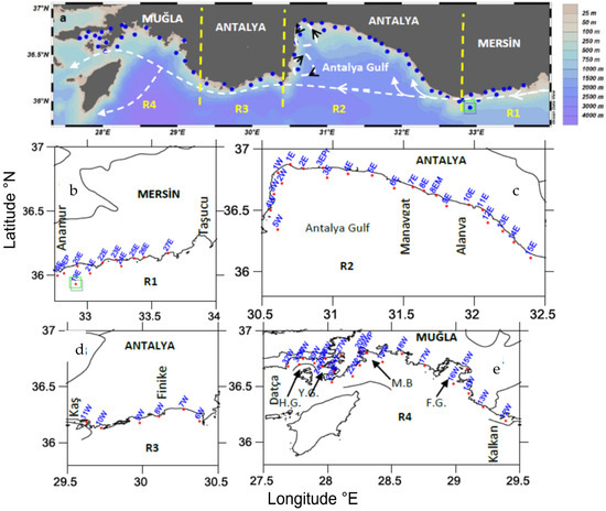
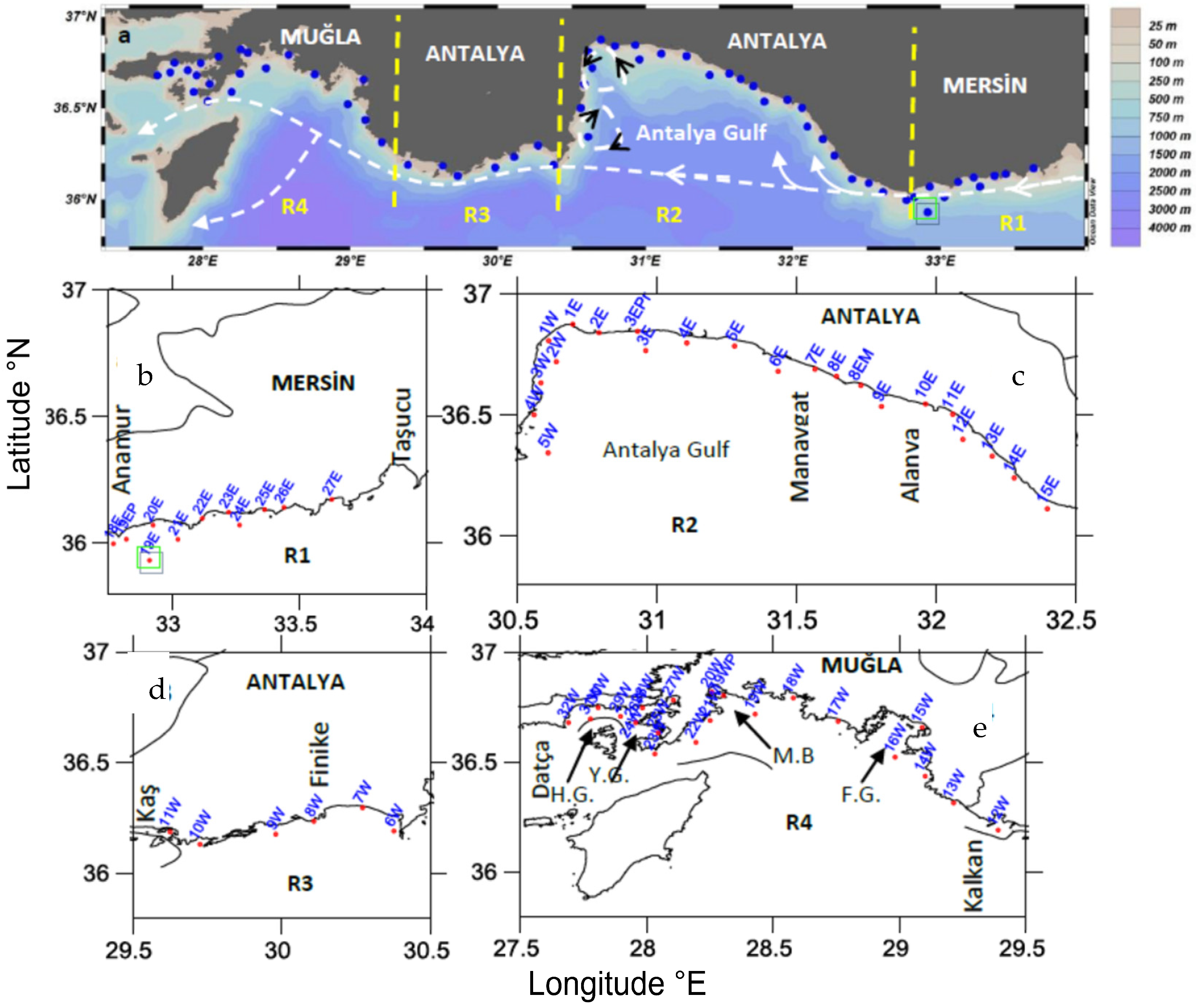
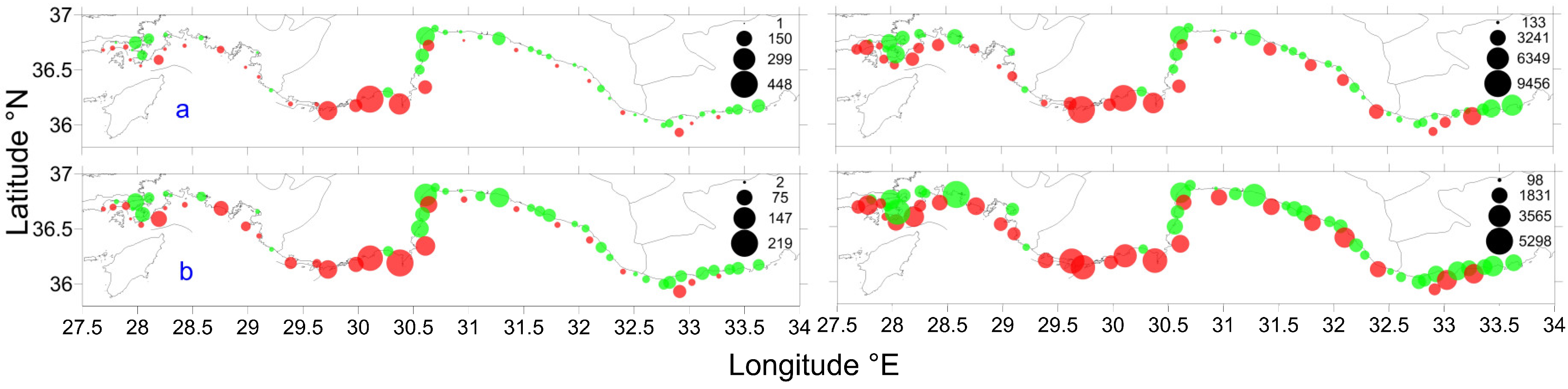
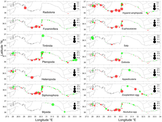
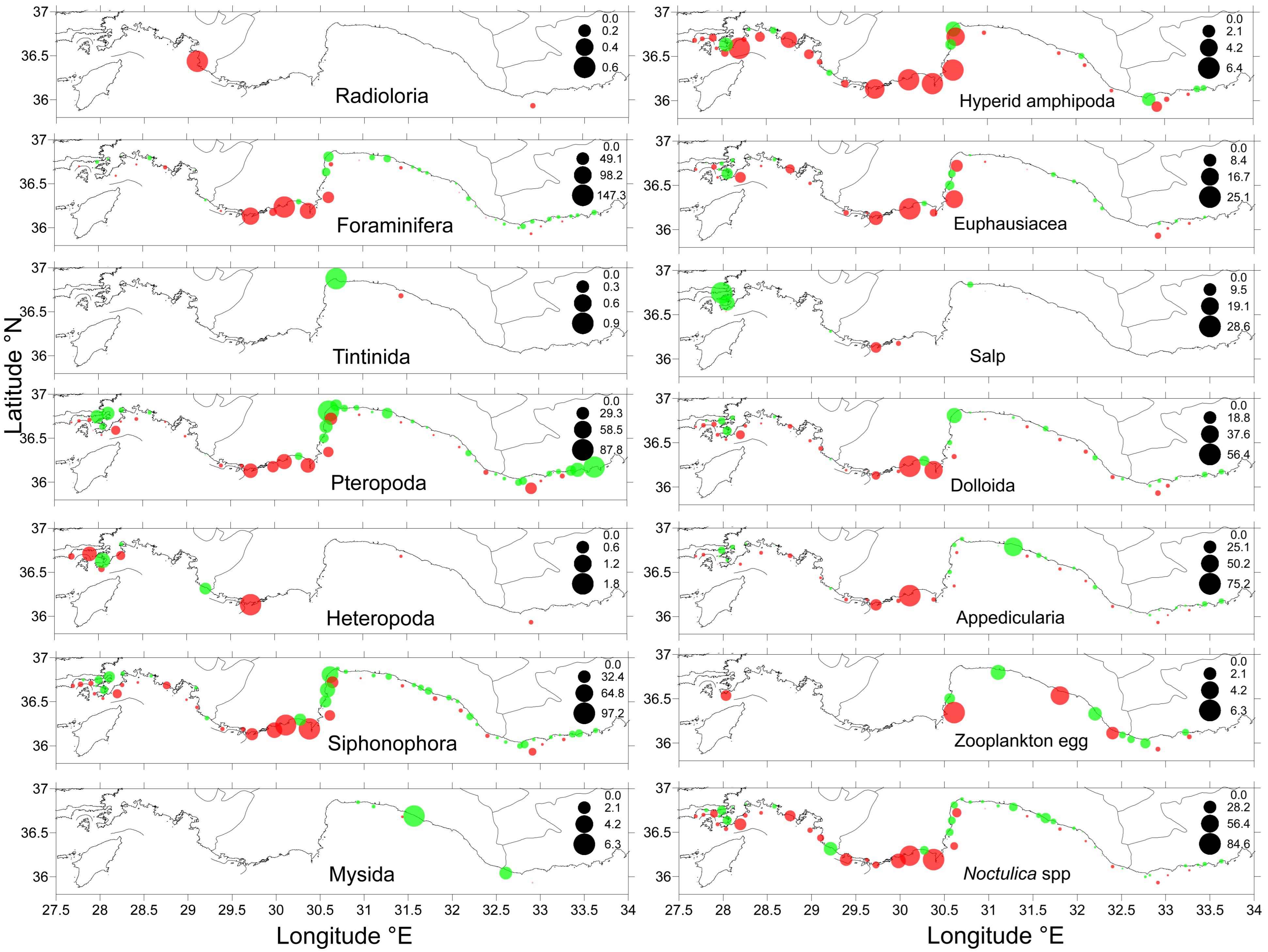
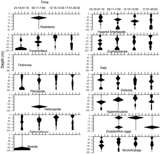
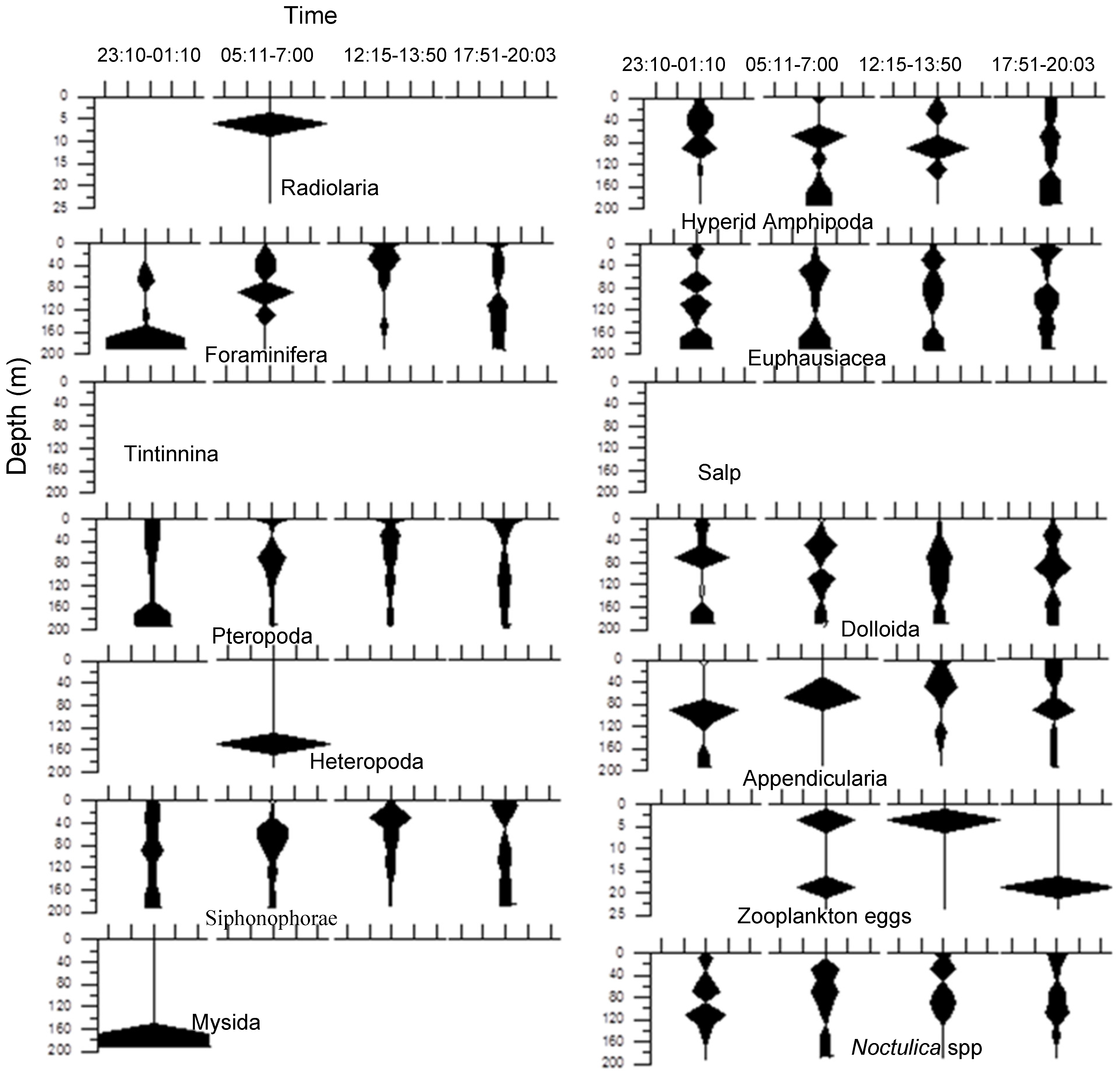
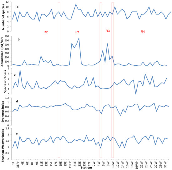
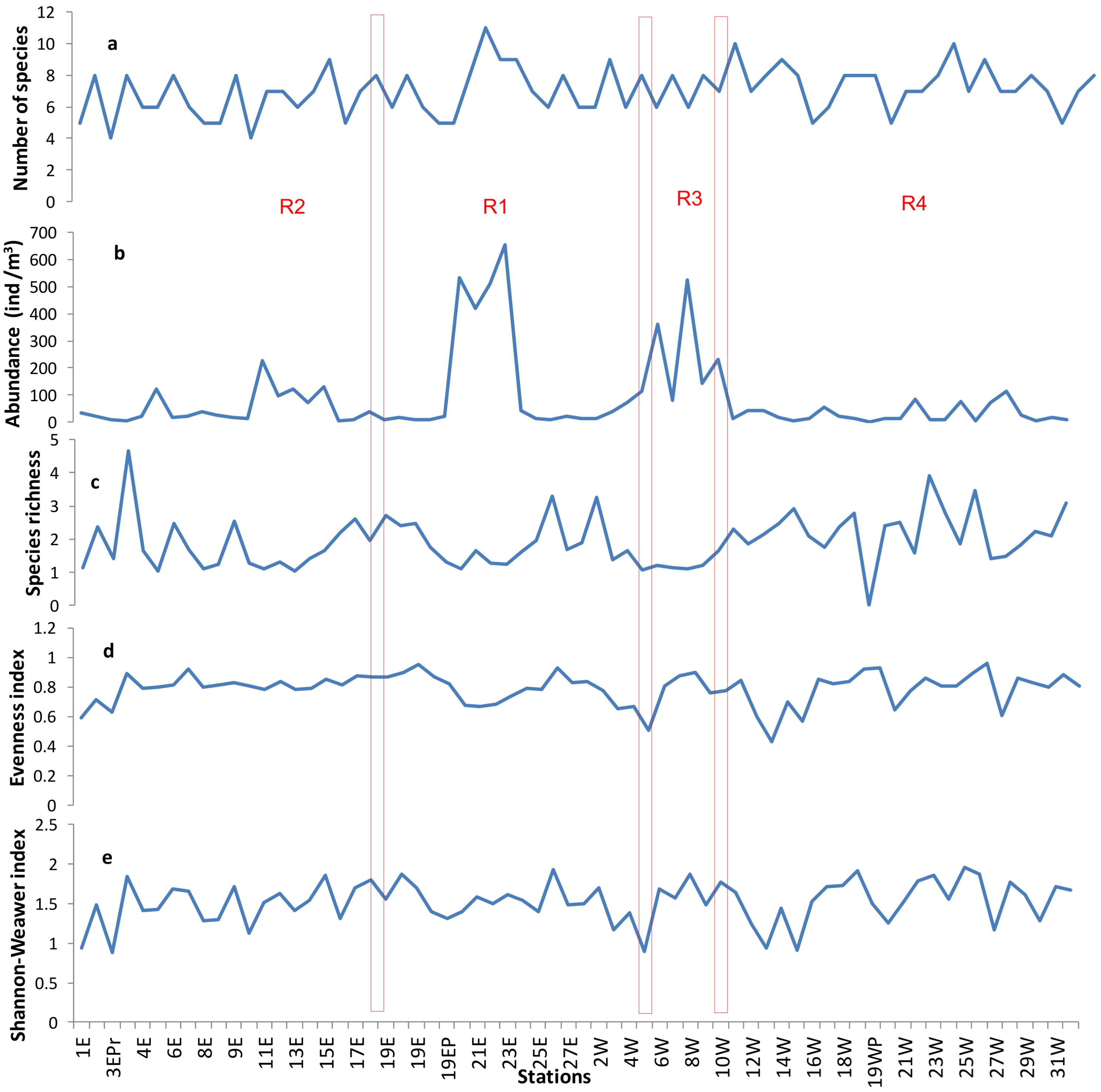
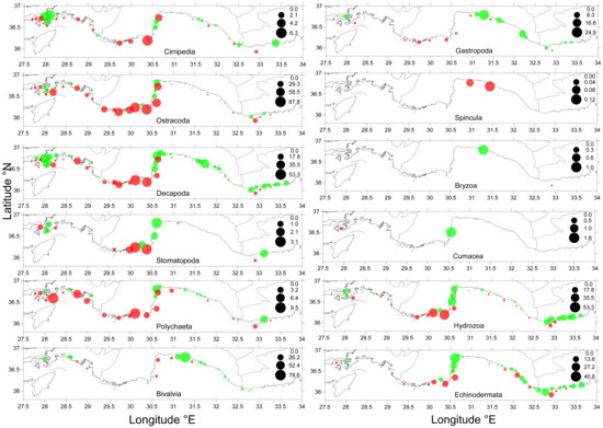
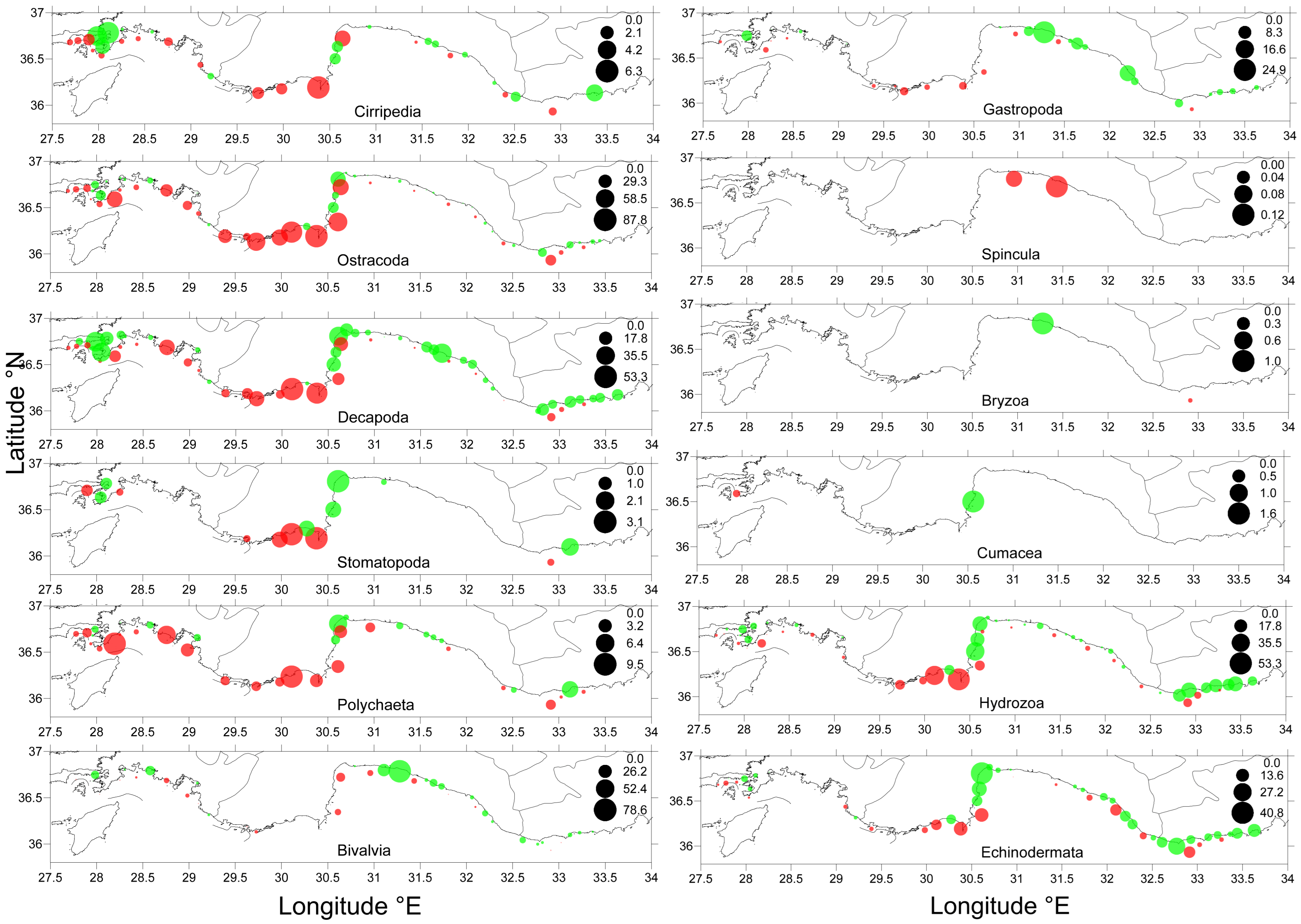
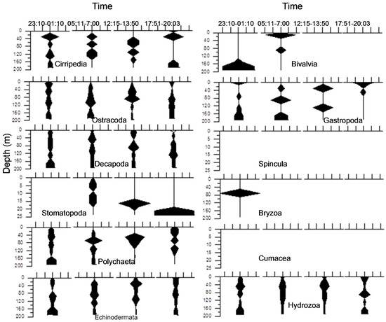
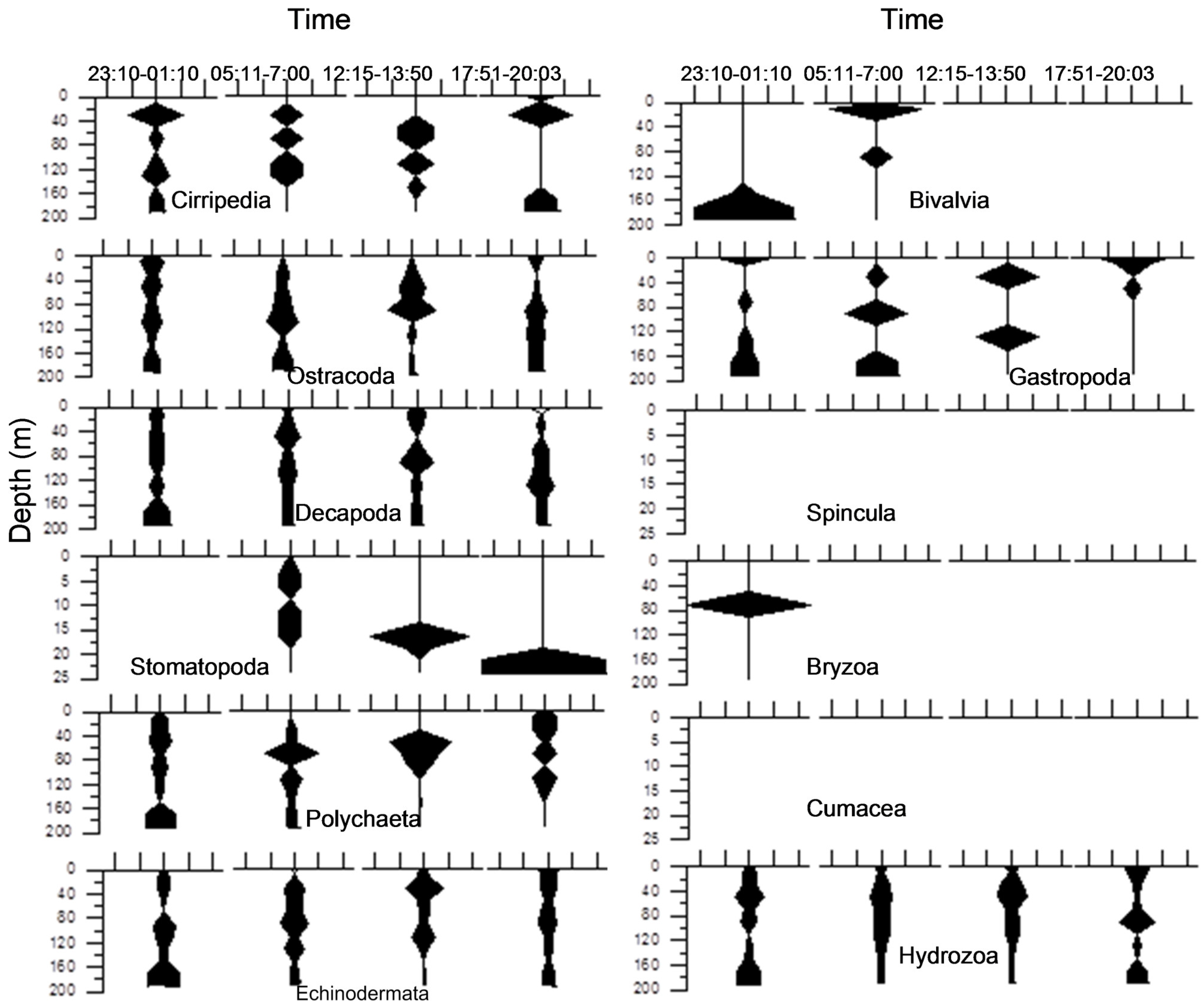
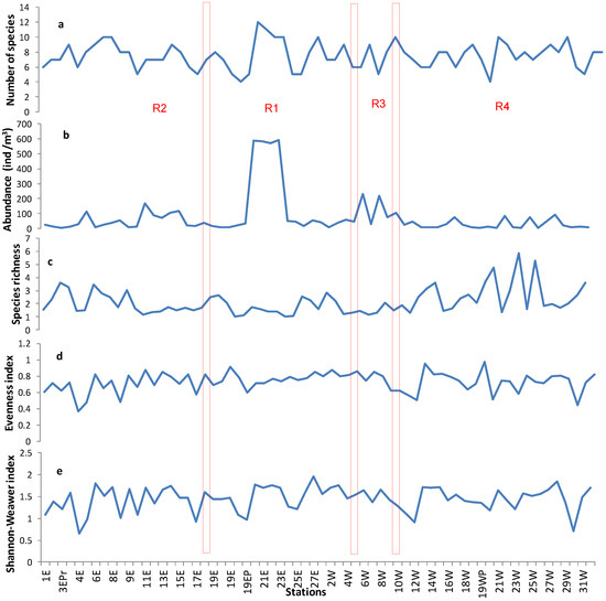
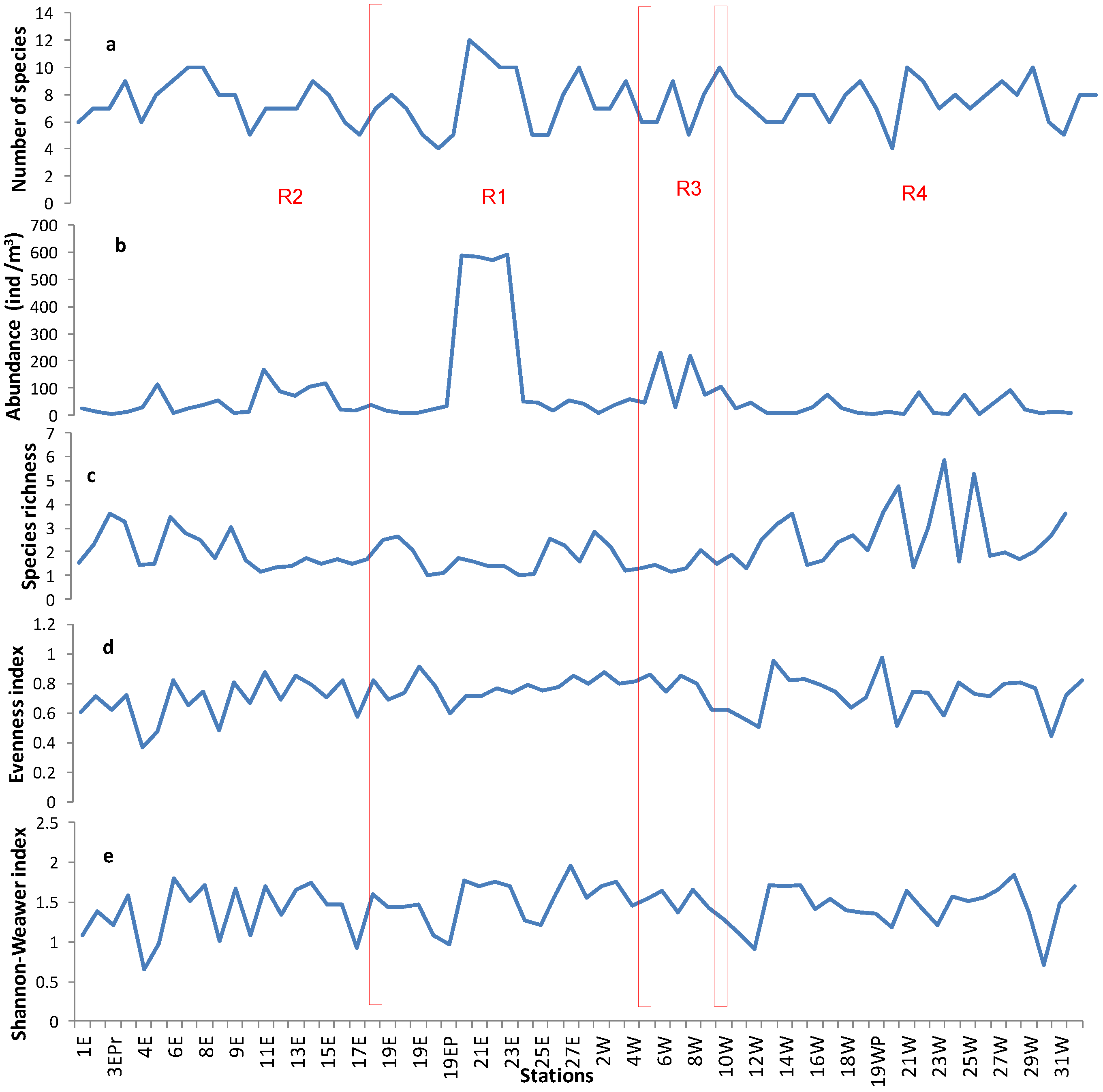
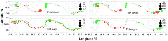
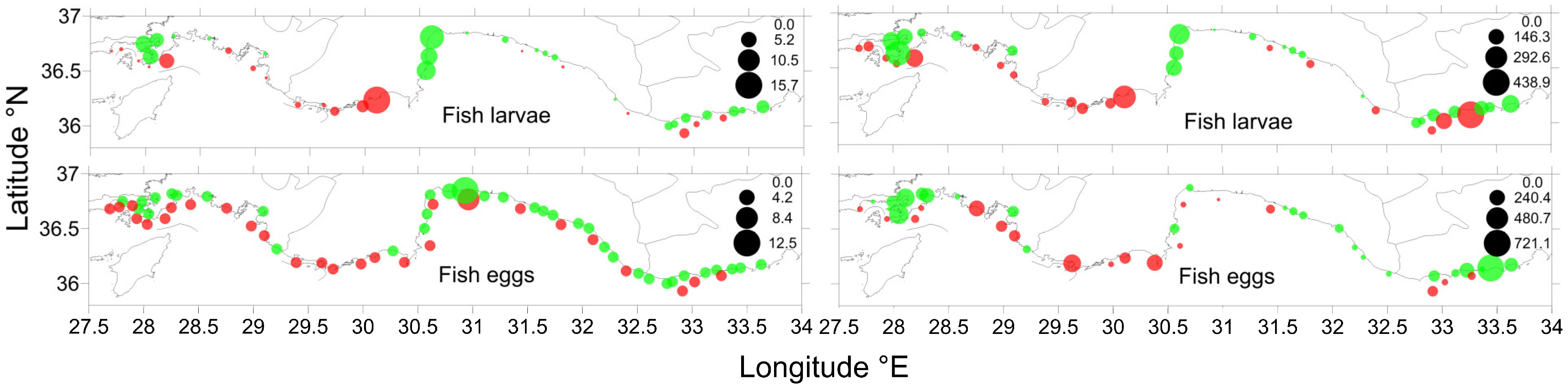
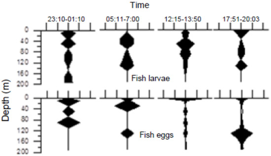
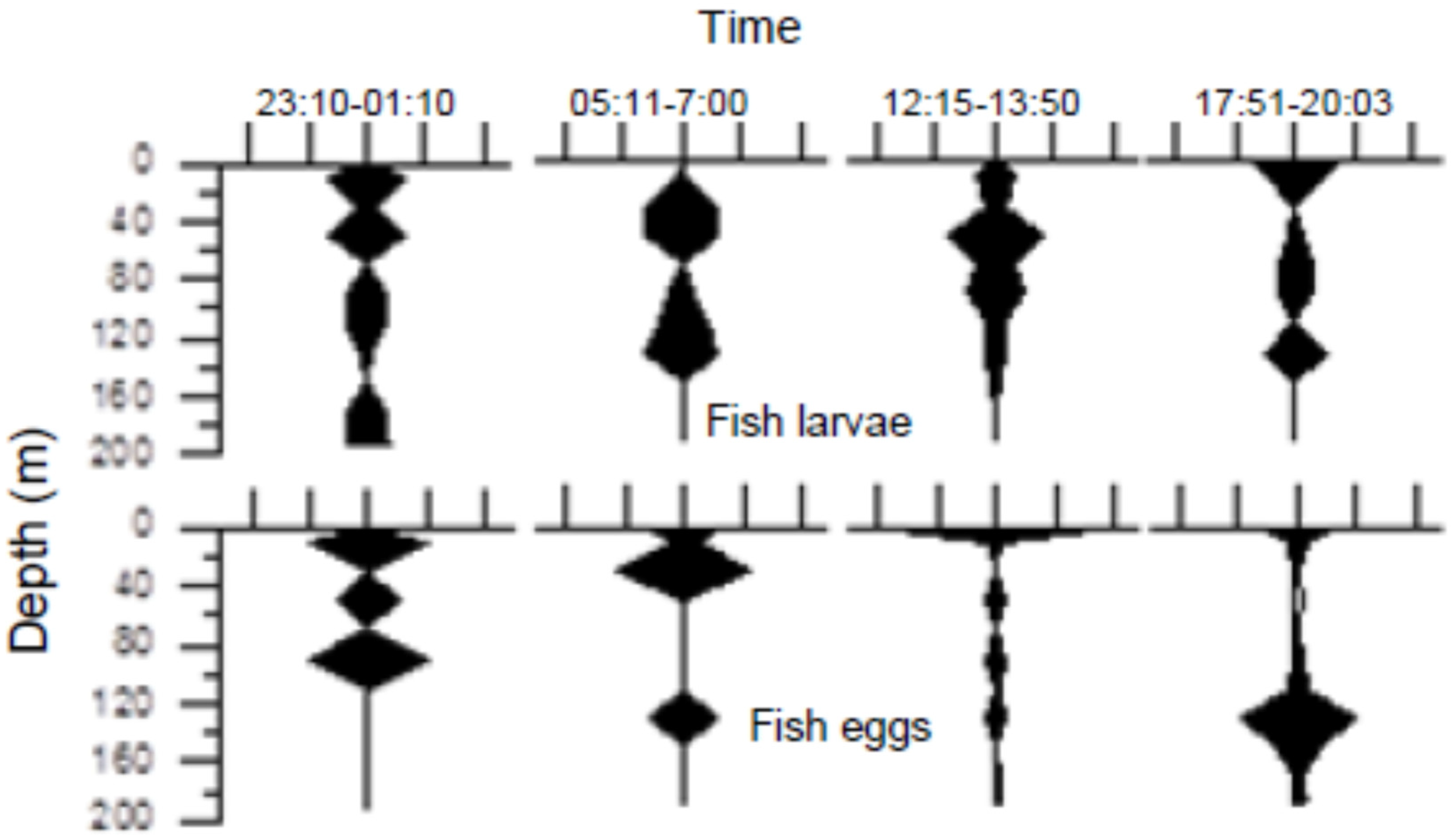

Disclaimer/Publisher’s Note: The statements, opinions and data contained in all publications are solely those of the individual author(s) and contributor(s) and not of MDPI and/or the editor(s). MDPI and/or the editor(s) disclaim responsibility for any injury to people or property resulting from any ideas, methods, instructions or products referred to in the content. |
© 2026 by the authors. Licensee MDPI, Basel, Switzerland. This article is an open access article distributed under the terms and conditions of the Creative Commons Attribution (CC BY) license.