


Abstract
The binding of transcription factors (TFs) to specific DNA sites plays a key role in regulating gene expression. Although experimental methods characterize binding motifs, their computational prediction directly from protein amino acid sequences remains an underexplored challenge. We developed prot2motif, a generative LSTM encoder–decoder model with additive attention that predicts a position probability matrix of the TF binding motif directly from the amino acid sequence and also generates an explicit “no motif” signal for non-TF proteins. The model was trained and evaluated on 3110 protein–motif pairs (1518 HOCOMOCO v13 TFs and 1592 length-matched non-TF proteins) partitioned using MMseqs2 clustering. Prot2motif successfully reconstructs binding motifs, substantially outperforming uniform baselines (SWscore 0.832 versus 0.625 on the TF subset); its generated output also enables reliable discrimination between TFs and non-TF proteins (F1 = 0.924), while shuffling amino acid residues within protein sequences reduced the classification F1-score to 0.647. Negative-control experiments confirmed that the model relies on the linear order of amino acid residues rather than composition alone, and that the learned motif signal strictly depends on correct protein–motif associations. Ablation analysis showed that the attention mechanism makes an important contribution to prediction quality, while non-autoregressive decoding is a viable alternative. Thus, in its current form, prot2motif provides reliable TF detection and motif generation for TFs.
1. Introduction
Transcription factors (TFs) are key regulators of gene expression and control various cellular processes through the specific recognition of DNA sequences. Determining the DNA-binding specificity of TFs is of fundamental importance for the study of regulatory networks, the annotation of functional genomic elements, and the interpretation of genetic variants in non-coding regions [1,2].
The specificity of TF–DNA interactions is typically described by a binding motif, since a single factor can recognize multiple related sequences with varying affinity. One of the most common representations of a motif is the position weight matrix (PWM), which characterizes the nucleotide distribution at each position. Such models are widely used for the identification of potential TF binding sites and are catalogued in large specialized databases, including HOCOMOCO and JASPAR [3,4].
Experimental determination of binding motifs is performed using ChIP-seq, HT-SELEX, protein binding microarrays, and other high-throughput technologies. Significant progress in this field was recently demonstrated in the Codebook study, in which Jolma et al. conducted 4804 experiments for 393 proteins and obtained new specificity models for many previously poorly characterized TFs. However, for a substantial fraction of the investigated factors, reliable binding models could not be obtained. This may be attributable to the dependence of binding for certain TFs on protein partners, post-translational modifications, and other biological conditions [5]. Thus, despite considerable progress in experimental methods, the comprehensive characterization of the binding specificity of all TFs remains an unsolved problem.
In parallel, computational methods for motif analysis have evolved from statistical de novo motif discovery algorithms, such as MEME, to deep learning approaches [6]. For example, DeepBind demonstrated the ability to predict the binding specificity of DNA- and RNA-binding proteins directly from experimental data [7]. However, most current methods formulate the task as predicting whether a given DNA sequence is bound by a specific TF. In such approaches, the amino acid sequence of the protein itself is generally not used as the primary source of information about its DNA-binding specificity.
Recent studies have demonstrated the promise of incorporating TF information into models of protein–DNA interactions. For instance, BTFBS utilizes the amino acid sequence of the TF jointly with the DNA sequence to predict their interaction [8], while TransBind integrates protein and DNA representations and demonstrates the advantages of this approach for binding site prediction, including prediction for TFs absent from the training set [9]. Additional opportunities are opened by the development of protein language models, such as ESM, which enable the extraction of contextual representations of amino acid sequences and the retrieval of information related to protein structure and function [10].
At the same time, the direct prediction of a DNA-binding motif from the amino acid sequence of a TF remains a distinct and insufficiently explored problem. Unlike the classification of predefined DNA segments, this formulation requires predicting the probability distribution of nucleotides at each motif position. It has previously been demonstrated that TF–DNA binding specificity can be predicted using structural information from protein–DNA complexes; however, the applicability of such methods is limited by the availability of experimentally determined structures [11]. Predicting the motif directly from the amino acid sequence of the protein potentially broadens the scope of such methods.
A related line of work predicts which residues of a protein contact DNA. CLAPE-DB combines the pre-trained protein language model ProtBert (ProtTrans checkpointRostlab/prot_bert; implementation v0.0.3) with contrastive learning to identify DNA-binding residues from sequence alone [12], and ProSiteHunter v1.0 integrates a fine-tuned protein language model with evolutionary, geometric and statistical sequence features to predict protein–DNA, protein–RNA and protein–protein interfaces in a single framework [13]. These methods answer a complementary question: where in the protein the DNA-binding interface lies, rather than which DNA sequence is recognised. Residue-level predictions are directly relevant to motif generation, because they could be used to restrict the encoder input to the predicted DNA-binding region and to reduce the influence of the long non-binding portions of TF sequences.
Structure-based modeling of protein–nucleic acid complexes provides a further source of information on the molecular basis of TF–DNA recognition. Cryo-EM in particular has become a major source of structures of such complexes, and a few deep-learning-based tools have been developed for their automated interpretation. ModelAngelo combines cryo-EM map information with protein sequence and structure in a graph neural network to build atomic models, including nucleotide backbones [14]. CryoREAD uses deep learning to locate phosphate, sugar and base positions in cryo-EM maps and traces them into de novo DNA and RNA models [15]. DEMO-EMol models protein–nucleic acid complexes by segmenting the cryo-EM map into protein and nucleic acid regions and fitting separately predicted chain models into them [16,17]. These methods reconstruct the three-dimensional structure of a complex from an experimental density map and do not predict the DNA sequence preferences of a TF. Nevertheless, together with structure-based predictors of binding specificity [11], they illustrate how structural information on protein–nucleic acid interfaces is becoming increasingly accessible, and they provide context for its potential integration into future DNA-binding motif prediction approaches.
In summary, modern experimental and computational methods enable effective characterization of transcription factor–DNA interactions; however, these approaches are primarily oriented toward obtaining or analyzing binding sites based on DNA sequence information or require additional protein structural data. The development of amino acid sequence representation methods, including protein language models, opens the possibility of directly leveraging protein information in the study of DNA-binding capacity. In this context, the task of directly predicting a TF DNA-binding motif from its amino acid sequence is of considerable interest, as it may complement existing approaches and expand the capabilities of computational transcription factor characterization.
2. Results
2.1. Evaluation of Prot2motif Performance and Comparison with Baseline Approaches
Two versions of the prot2motif model were compared in this study. The prot2motif_small model was trained on positive examples only, and the validation set also contained only transcription factors, whereas prot2motif_big was trained on a combined set of positive and negative examples. A unified test set containing both transcription factors and negative examples was used for the final evaluation, ensuring comparability of results. The final metric values are presented in Table 1.
Table 1.
Quality assessment results for models and baselines.
Four metrics reflecting different aspects of agreement between the predicted and reference motifs were used for quality assessment. SWscore and the symmetric KL divergence (KLdiv_sym) characterize the direct similarity of corresponding elements of the two matrices and can therefore be considered primarily as technical indicators of reference reproduction accuracy. On the full test set, the SWscore and KLdiv_sym for prot2motif_small were 0.771 and 4.99, respectively, whereas for prot2motif_big they were 0.905 and 1.762.
SWscore is sensitive to correct motif length determination, since padding positions are also included in the comparison. Therefore, an error in motif boundary determination reduces the final score even when the nucleotide specificity within the motif itself is correctly reproduced. In contrast, the Motif Similarity metric permits optimal local alignment of the predicted and reference motifs, reducing the dependence of the score on their relative positions. However, such alignment may fall on low-conservation regions of limited biological significance. This is particularly evident for negative examples, for which Motif Similarity reaches values close to unity (0.999 and 1.0 for the small and big models, respectively), despite the absence of an informative motif.
To address this limitation, the Normalized SWscore metric was developed, in which the contribution of each position is determined by its information content. For positive examples, the values were 0.721 for prot2motif_small and 0.727 for prot2motif_big. For negative examples, Normalized SWscore equals zero, since the reference matrices contain no nucleotide specificity and have zero information content. Thus, this metric accounts not only for the degree of matrix agreement but also for the biological informativeness of the aligned motif positions.
Comparison with baselines demonstrates that both models outperform simple strategies on the transcription factor subset. The SWscore for prot2motif_small was 0.839, and for prot2motif_big, 0.832, compared to 0.625 and 0.616 for baseline_1 and baseline_2, respectively. A similar advantage was observed for Normalized SWscore: 0.721 and 0.727 for the small and big models versus 0.658 and 0.646 for the baselines. For KLdiv_sym, where lower values correspond to greater matrix similarity, both models also substantially outperformed the baselines: 2.877 and 2.997 versus 10.663 and 10.703. However, the advantage of the models in terms of Motif Similarity is considerably less pronounced (0.824 and 0.828 versus 0.817 and 0.809), which is consistent with the limited ability of this metric to distinguish biologically meaningful motif similarity.
Thus, comparison with baselines demonstrates that the models utilize protein sequence information to predict motif nucleotide specificity. The differences between the small and big models are most pronounced on negative examples: prot2motif_big, trained with negative samples, exhibits a substantially lower KLdiv_sym (0.526 versus 7.103) and a higher SWscore (0.978 versus 0.704). Collectively, the results indicate that the inclusion of negative examples enables the model to better reproduce the absence of motif specificity while maintaining comparable motif prediction quality for transcription factors.
2.2. Negative Controls: Sequence Shuffling and Permuted Protein–Motif Pairs
To elucidate the specific information extracted by the model from the primary protein sequence, we compared prot2motif_big against two negative control settings. In the first control (amino acid shuffling), the test sequences were subjected to random permutation of their residues. This procedure preserved both sequence length and amino acid composition, thereby disrupting the linear order while retaining global compositional features. In the second control (complete pair shuffling), the model was trained on a dataset in which the correspondence between protein sequences and target motifs was entirely randomized across all entries, whereas the test set remained unaltered. All models were trained using random seed 42; the tables report (Table 2 and Table 3) below.
Table 2.
Comparison of the quality of motif generation between the basic model and negative control (Shuffled aa residues, Fully shuffled protein–motif pairs).
Table 3.
Comparison of the quality of motif classification between the basic model and negative control (Shuffled aa residues, Fully shuffled protein–motif pairs).
Analysis of the results indicates that the random permutation of amino acids leads to a substantial decrease in performance for both motif generation and classification. Since this shuffling procedure preserves both protein length and amino acid composition, the observed drop in metrics (particularly ROC AUC and SWscore for TFs) demonstrates that the model relies on the linear order of amino acid residues rather than solely on their composition. Meanwhile, the prediction quality for non-TFs remains virtually unchanged, confirming that the overall performance degradation is driven specifically by the loss of ability to recognize TFs and generate their specific motifs upon disruption of the primary sequence. Notably, the ROC AUC in this control remains substantially above the chance level, indicating the presence of residual compositional features that allow for partial discrimination between TFs and non-TFs even when the residue order is disrupted.
Under the conditions of complete protein–motif pair shuffling, the statistical association between the input sequence and the target variable is entirely absent at both the protein class level and the specific motif level. In such a scenario, the optimal strategy for minimizing the loss function is to output an averaged (nearly uniform) probability distribution. This is precisely the behavior exhibited by the model: the ROC AUC drops to the chance level, and the F1-score drops to zero, as this averaged prediction is interpreted as the absence of a motif for all proteins. The decrease in generation metrics (SWscore, KLdiv) across both classes confirms that the model loses its capacity to extract specific patterns, degenerating into a trivial baseline prediction.
The interpretation of the Motif_similarity and Normalized_SW metrics, which show negligible differences between the primary model and the negative controls, warrants special attention. The Motif_similarity metric permits optimal local alignment of the predicted and reference motifs, which reduces the score’s dependence on their exact positioning but may lead to a formal inflation of the score through matches with low-conservation regions lacking biological significance. The Normalized_SW metric was developed to address this limitation: it accounts not only for the degree of matrix agreement but also for the biological informativeness of the aligned positions, as determined by their information content. For negative examples (non-TFs), it is undefined (or equals zero), as the reference matrices contain no nucleotide specificity.
The stability of these metric values for TFs across all three models indicates that even upon degradation of predictive performance (e.g., when outputting an averaged distribution), the local alignment algorithm finds a formal match with the reference, and the final Normalized_SW score largely reflects the contribution of the reference motif’s own information content. Consequently, these metrics are less sensitive to the model’s loss of ability to correctly determine motif boundaries and discriminate between protein classes. Therefore, the true capacity of the model to extract sequential features and generate biologically meaningful patterns is reliably assessed only through the SWscore and KLdiv_sym metrics (which account for the ‘no motif’ channel), as well as the classification metrics.
2.3. Ablation Analysis of the Prot2motif Architecture
To assess the contribution of key architectural components to the quality of motif creation, an ablation study was conducted. In particular, we investigated the effect of switching to non-autoregressive forecasting (abl_nonar) and the complete removal of the attention mechanism (abl_no_attn) compared to prot2motif_big. The evaluation was performed on a tested subset of transcription factors (TFs) (Table 4). It should be noted that the ability of the models to classify proteins as TFs or non-TFs was not considered in this ablative analysis. The focus of the study was solely on indicators of motive generation.
Table 4.
Motif generation metrics for ablation variants on the tefocuss).
The transition to the non-autoregressive variant (abl_nonar) does not lead to a degradation of overall predictive performance. A statistically significant, albeit moderate, change in the technical metrics is observed: the SWscore decreases from 0.832 to 0.815 (two-sided Wilcoxon test for the TF subset, p < 0.001), while the symmetric Kullback–Leibler divergence (KLdiv_sym) increases from 2.997 to 3.320. At the same time, the Motif_similarity metric remains at a comparable level (0.822 vs. 0.828) and Normalized_SW demonstrates growth from 0.727 to 0.823. These results indicate that step-by-step generation with autoregressive feedback is not a strictly necessary condition for solving the task. The non-autoregressive architecture demonstrates comparable prediction quality, suggesting the fundamental feasibility of directly mapping the global feature representation of a protein onto the motif matrix without using a sequential decoder. The Motif_similarity and Normalized_SW metrics remain at levels close to those of the reference model, confirming the preservation of the ability to reproduce the nucleotide specificity of motifs. Thus, both architectural configurations successfully handle the motif prediction task, demonstrating the flexibility of the approach and the absence of a rigid dependence of quality on the generation mechanism.
In contrast, the complete removal of the attention mechanism (abl_no_attn) leads to a degradation of all generation quality metrics. The SWscore decreases to 0.745 (p < 0.001), and KLdiv_sym increases to 5.205 (p < 0.001).
This collapse is caused by a fundamental limitation of this configuration: in the absence of an attention mechanism, the only channel for transmitting information from the encoder to the decoder is the final hidden state of the recurrent network. As a result, network’s state converges to a constant, completely “washing out” protein-specific features. The decoder receives a nearly identical initial vector for any input sequence and loses the ability to generate specific motifs. This result emphasizes that in encoder–decoder architectures without an attention mechanism, correct handling input data is a strict prerequisite for model functionality.
2.4. Latent Space Structure and Protein Classification
Additionally, the structure of the latent representations of the final prot2motif_big model was investigated. Since the model was trained on a mixed dataset containing both transcriptional and non-transcriptional proteins, the hidden states could contain features related to functional protein classification. To test this hypothesis, a binary LogisticRegression classifier was trained on the decoder hidden states to separate proteins into two classes: TF and non-TF. On the test set, the classifier achieved an F1-score of 0.924, indicating that the latent representations contain information sufficient to discriminate between the two classes.
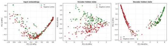
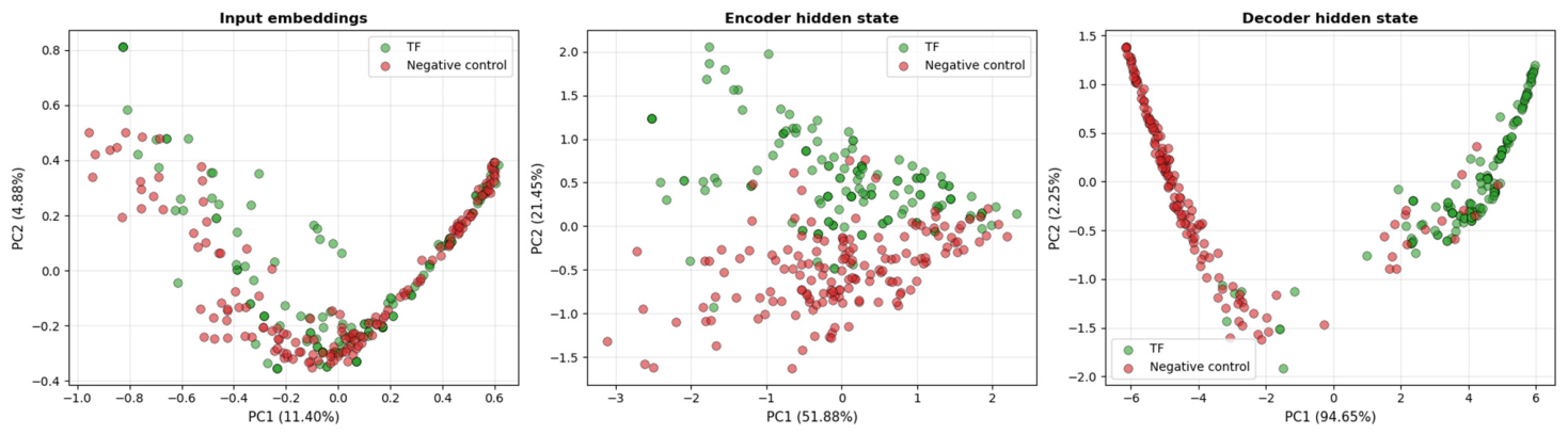
The structure of the decoder hidden space of the final model (decoder_hidden) was further assessed using the silhouette coefficient and visualization of the latent representations by principal component analysis (PCA). Figure 1 presents two-dimensional projections of the hidden states for transcriptional and non-transcriptional proteins at various stages of sequence processing. The visualization shows that as information propagates through the model architecture, the distinction between the two functional classes becomes more pronounced.
Figure 1.
PCA visualization of the hidden states of the prot2motif model.
Quantitative assessment of class separability is presented in Table 5. The silhouette coefficient for the input embeddings (Embedded Input) was 0.0025, for the encoder hidden states (encoder_hidden) it was 0.1242, and for the decoder hidden states (decoder_hidden) it increased to 0.6253. Thus, the most pronounced separation of TFs and non-TFs was observed in the decoder space, which is consistent with the clustering pattern observed in the corresponding PCA visualization.
Table 5.
Clustering results for the hidden states of the prot2motif model.
These results demonstrate that the latent representations of the final model contain information related to the functional classification of proteins. The increase in the silhouette coefficient from the encoder to the decoder may indicate further formation of distinctions between TFs and non-TFs during sequential motif generation.
2.5. Identification of Potential Transcription Factors and Binding Sites
As a result of human proteome screening, the binary classifier assigned 5156 protein sequences as potential transcription factors. For these sequences, putative DNA-binding motifs were generated, and their occurrences were searched in EPDnew promoter sequences using FIMO. After filtering by statistical significance (q < 0.05), 634 proteins were selected for which at least one statistically significant site corresponding to the predicted motif was identified in promoter sequences.
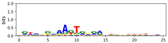
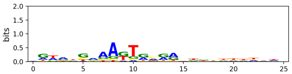
As an example of a potential biological application of the developed approach, the HLA-DRA gene, associated with bronchial asthma, was examined. A statistically significant site corresponding to the motif predicted for protein Q8N718, classified as a transcription factor by the classifier, was identified in its promoter region. Figure 2 shows the logo representation of the predicted motif.
Figure 2.
Logo representation of the predicted motif for protein Q8N718. Nucleotides are colour-coded as follows: A—blue, C—yellow, G—green, T—red.
This result should be regarded as a computational hypothesis regarding the potential involvement of Q8N718 in the regulation of HLA-DRA expression, requiring subsequent experimental validation.
3. Discussion
In this study, we developed prot2motif, a generative encoder–decoder model capable of detecting transcription factors (TFs) and predicting positional frequency matrices of DNA-binding motifs directly from protein amino acid sequences. Negative control experiments confirmed that the model relies on the linear order of amino acid residues and forms meaningful protein-specific representations, successfully reconstructing binding motifs.
The evaluation of motif generation quality highlights the importance of metric selection. Position-wise metrics (SWscore, KLdiv_sym) and local alignment-based metrics (Motif_similarity, Normalized_SW) capture different aspects of prediction performance. The model demonstrates the ability to reproduce the nucleotide specificity of motifs, as evidenced by its superior performance over baseline approaches.
The ablation analysis provided important insights into the architectural requirements of the model. The complete removal of the attention mechanism and context vector reduces prediction quality, indicating the necessity of aggregating information across the entire protein sequence rather than relying solely on a compressed final hidden state. At the same time, transitioning to a non-autoregressive decoder, which predicts the entire motif matrix in a single pass, demonstrates performance comparable to the reference model. This suggests that the non-autoregressive approach can indeed be useful for this task; however, its potential and optimal integration mechanisms require separate, dedicated investigation in future work.
Analysis of the latent space revealed that during motif generation, the model implicitly forms representations that reliably separate TF and non-TF classes. The application of prot2motif for human proteome screening enabled the formulation of novel hypotheses regarding regulatory interactions.
Nevertheless, studying has several limitations. Sequence clustering with an 85% identity threshold effectively mitigates close homolog leakage; however, the current performance reflects the model’s generalization capability within already characterized TF families. Promising directions for future work include integrating residue-level DNA-binding predictions (e.g., using ProSiteHunter [13] or CLAPE-DB [12] approaches) to focus the encoder on functional domains, as well as employing protein language model embeddings. Structural information on protein–nucleic acid complexes, which is becoming increasingly accessible owing to cryo-EM-based modeling tools such as ModelAngelo [14], CryoREAD [15], and DEMO-EMol [16,17], could also be integrated into future versions of the model, for example to guide the prediction of the DNA-binding interface and thereby complement the sequence-based approach. Finally, computational predictions require integration with biological context data for definitive experimental validation.
4. Materials and Methods
4.1. Dataset
Protein–binding site motif pairs were used for model training and evaluation. The initial set of transcription factors (TFs) was compiled from the HOCOMOCO v13 database, which contains experimentally derived and curated binding models for human and mouse TFs [3]. At the time of dataset construction, the database contained 1611 human TF–motif pairs. To increase the homogeneity of the positive class, motifs with a length of up to 26 nucleotides were retained, yielding 1592 TF–motif pairs.
Data partitioning into training, validation, and test sets was performed at the level of protein sequence clusters to prevent information leakage. Sequence clustering was executed using MMseqs2 [18] with the following parameters: a sequence identity threshold of 85% (‘–min-seq-id 0.85’), an E-value threshold of 10−3 (‘-e 0.001’), an alignment coverage threshold of 80% (‘-c 0.8’ with ‘–cov-mode 0’, requiring coverage of both sequences), and the greedy set-cover clustering algorithm (‘–cluster-mode 0’). Subsets were constructed such that sequences from the same cluster were never assigned to different splits. All TF–motif pairs corresponding to a single protein were assigned to the same split. The resulting clusters were randomly distributed among the training, validation, and test sets in an 80%, 10%, and 10% ratio, respectively.
An 85% identity threshold was selected as an optimal compromise between minimizing homology leakage and maintaining sufficient data density for deep learning. During preliminary experiments, we varied the clustering threshold from 0.20 to 0.90. While stricter thresholds (e.g., 50–60%) would provide more rigorous separation of homologs, they resulted in a critical reduction in the training set size and a loss of representativeness across diverse TF families. This data scarcity severely hindered the convergence of the LSTM-based generative model. Therefore, the 85% threshold was chosen to effectively remove close homologs from the test set while retaining the statistical power required for robust model training and generalization.
Following the formation of splits for the positive class, negative examples (non-TFs) were independently added to each subset. For this purpose, human protein sequences were selected from UniProt based on the following criteria: (1) a length of up to 1024 amino acids (inclusive); (2) the absence of the keyword “Transcription” [KW-0804]; (3) the absence of the Gene Ontology term GO:0003700 (DNA-binding transcription factor activity); and (4) the absence of the Gene Ontology term GO:0006355 (regulation of DNA-templated transcription). For each split, non-TF proteins were sampled using stratified sampling to match the length distribution of the TFs within that specific split. The length range was divided into 50-amino-acid bins, and for each bin, a random subset of non-TF proteins equal in size to the number of TFs in the corresponding bin was selected (i.e., one non-TF protein per TF–motif pair).
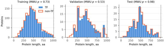
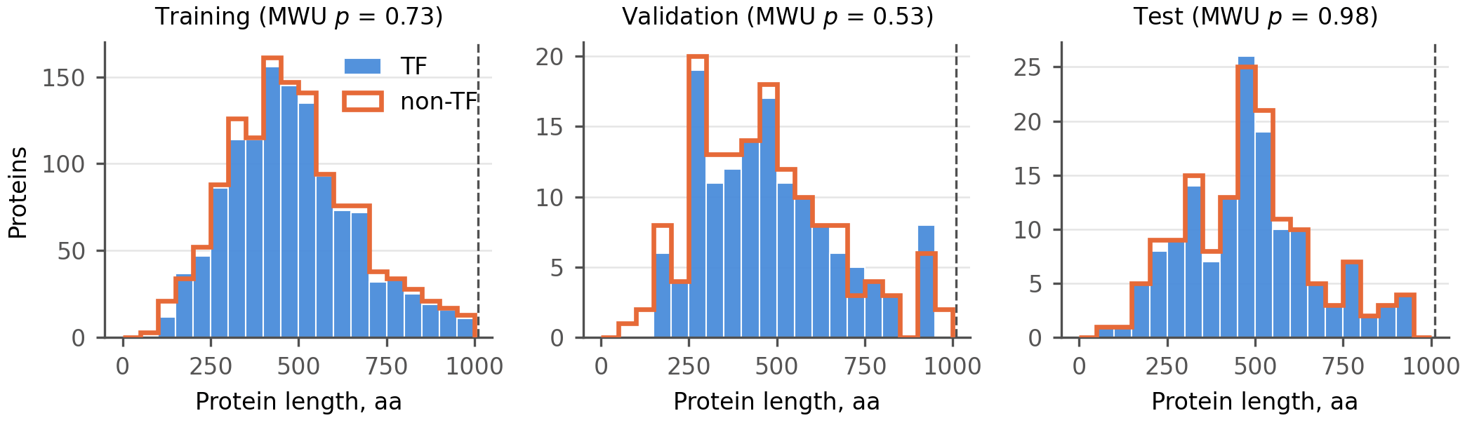
Length matching was performed prior to applying the final 1024-residue filter to the positive class. Because this filter removed a greater number of long TFs than non-TFs, the final dataset comprises 1518 TF–motif pairs and 1592 non-TF proteins (Table 6). The resulting length distributions for the two classes are statistically indistinguishable across all splits (Mann–Whitney U test; Figure 3).
Table 6.
Dataset sizes.
Figure 3.
Protein length distributions of transcription factors (TFs) and non-TF proteins across data splits. Histograms show the distribution of protein sequence lengths (in amino acids, aa) for the positive class (TFs, blue filled bars) and the negative class (non-TFs, orange outlined bars). The data is presented separately for the Training, Validation, and Test sets. To eliminate length-related bias, negative examples were selected using stratified sampling to match the length distribution of TFs within each split. The distributions of the two classes are highly overlapping in all three subsets. Mann–Whitney U (MWU) test p-values are indicated in the titles of each panel (p = 0.73, p = 0.53, and p = 0.98, respectively), demonstrating no statistically significant difference in the lengths of TFs and non-TFs. The dashed vertical line at 1024 aa indicates the maximum sequence length threshold applied during dataset construction.
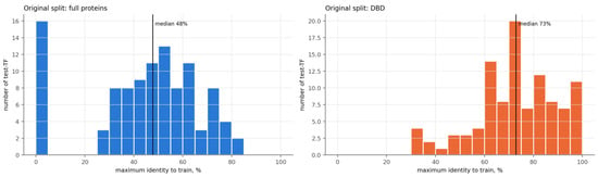
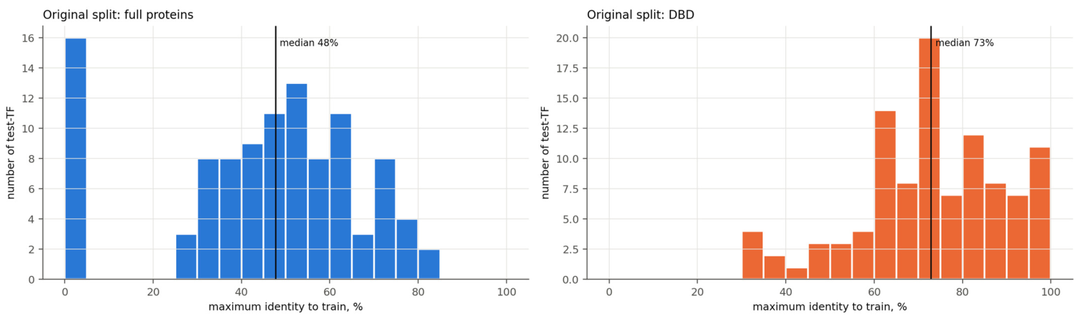
To quantitatively assess the similarity between the training and test sets, an analysis of the maximum percentage identity of each test TF against the proteins in the training set was conducted (Figure 4). Analysis of the full-length sequences (Figure 4 left) reveals a satisfactory distribution: the median maximum identity is 48%, and no test protein shares a close homolog (>85% identity) with the training set, thereby confirming the appropriateness of the chosen clustering threshold. Conversely, an analysis of similarity restricted exclusively to DNA-binding domains (DBDs) (Figure 4 right) demonstrates an expected shift toward higher values (median: 73%). This high DBD similarity between the test and training sets is biologically inherent: the number of evolutionarily conserved DBD families is limited, and the domains themselves are relatively short (ranging from a few dozen amino acids depending on the family), which statistically increases the probability of cross-sample similarity.
Figure 4.
Sequence identity distribution of test transcription factors (TFs) to the training set for full-length proteins and DNA-binding domains (DBDs). The histograms show the distribution of sequence identity (in %) of each test TF to the training proteins. The x-axis represents the identity to the training set, and the y-axis shows the number of test TFs. (left) Distribution for full-length proteins (blue bars). The median identity is 48%. (right) Distribution for DNA-binding domains (DBDs) (orange bars). The median identity is notably higher at 73%.
4.2. Motif Preparation and Representation
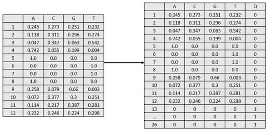
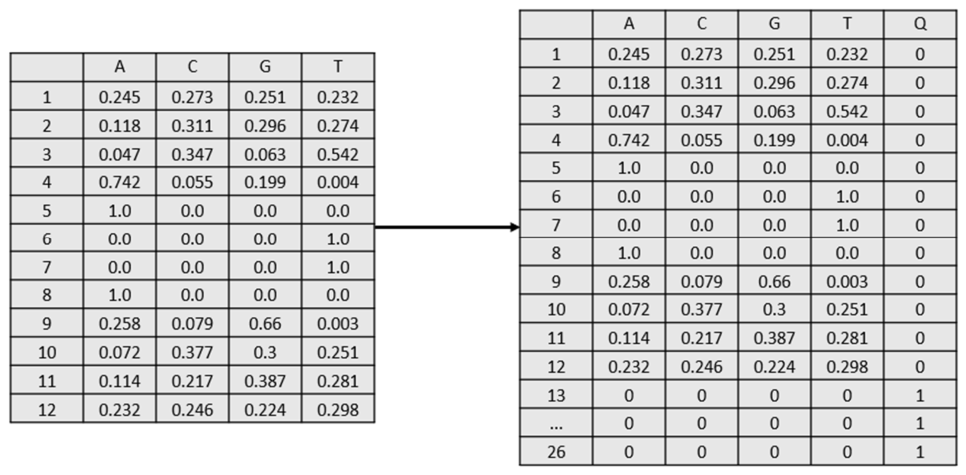
Target motifs were represented as nucleotide probability matrices. Since motif lengths varied, all matrices were padded to a common maximum length of 26 nucleotides. Shorter motifs were padded with zero-filled rows.
A special fifth symbol, not corresponding to any standard nucleotide, was introduced to denote the end of the motif. For actual motif positions, the value of this symbol was set to zero, whereas for padding rows, it was set to one. Thus, the model output was a fixed-length matrix with five components at each position: A, C, G, T, and a sequence termination token Q. Figure 5 illustrates an example of motif preprocessing.
Figure 5.
Original (left) and unified (right) motif matrices for ARX.H13CORE.1.SM.B.
4.3. Architecture of Prot2motif
We developed a generative model, prot2motif, implemented according to the encoder–decoder paradigm [19]. This architecture is well suited to our task, as it accounts for the sequential nature of both the input protein sequences and the output motif matrices.
The encoder receives the amino acid sequence of the transcription factor, tokenised as the 20 standard amino acids (indices 1–20), an unknown-residue token and a padding token (index 0). Sequences are padded with the padding token to a fixed length of 1024; no sequence exceeded this length after filtering. Tokens are mapped by a trainable embedding layer of dimension equal to the hidden size (256), followed by dropout (p = 0.2) and a single-layer, unidirectional LSTM that produces a hidden state for every position. In the reported models, padding positions are not masked: the encoder processes the full padded sequence and attention is computed over all 1024 positions.
The decoder is a single-layer unidirectional LSTM initialised with the final hidden and cell states of the encoder. It generates the motif matrix in exactly 26 steps; at each step, it outputs a distribution over five symbols (A, C, G, T and the end-of-motif symbol Q), giving a 26 × 5 matrix. The input of the first step is a zero vector, and the input of every subsequent step is the softmax of the previous output, projected to the hidden size by a linear layer and concatenated with the attention context vector. The same procedure is used during training and inference. The model has 1.71 million trainable parameters for a hidden size of 256.
Information transfer from the encoder to the decoder was implemented using the additive attention mechanism of Bahdanau et al. [19]. At each decoding step, a compatibility score is computed between the current decoder hidden state and the hidden states of all amino acids in the protein:
where Wa, Ua, and Va are trainable weight matrices, si−1 is the decoder hidden state at the previous step, and hj is the encoder hidden state for the j-th amino acid. After normalization of the scores with the softmax function, the attention weights are obtained:
where d is the length of the protein amino acid sequence. The computed attention weights are used to calculate the context vector:
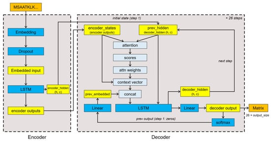
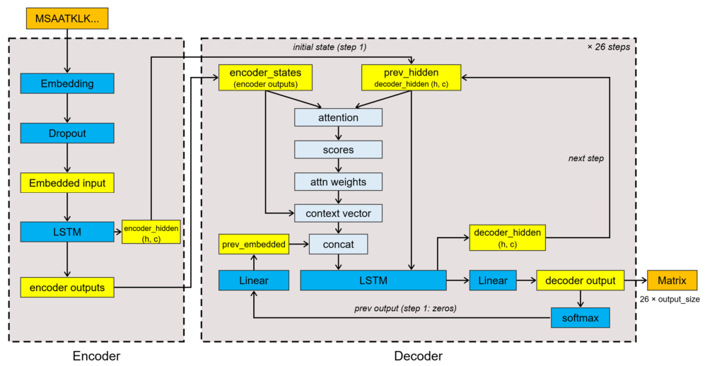
A single set of attention weights is used for each generation step in the model; multi-head aggregation is not applied. The resulting context vector is passed to the decoder to form the probability distribution at the current motif position. The architecture of our model is presented in Figure 6.
Figure 6.
Architecture of the prot2motif model. Schematic of the LSTM-based model with attention: the encoder transforms the amino acid sequence into a set of representations, and the decoder constructs the output matrix from them in 26 steps. At each step, attention selects the relevant positions of the sequence, and the output of the previous step is fed back as input.
4.4. Loss Function
Model training was formulated as the minimization of the divergence between the reference motif matrix and the predicted probability matrix. The Kullback–Leibler (KL) divergence was used as the loss function:
where L is the motif length, pi(b) is the probability of nucleotide b at position i in the reference matrix, qi(b) is the probability of nucleotide b at position i in the generated matrix, and A = {A,C,G,T,Q}.
For each motif position, the loss characterizes the deviation of the predicted nucleotide probability distribution from the reference distribution. The final loss value was computed by averaging over motif positions.
4.5. Model Training
The model was trained using the AdamW optimizer (initial learning rate—0.005, decay rate—0.01), with gradient clipping to a norm of 1.0 and using mini-batches of 32 samples selected at random. Protein sequences of variable length are padded to a fixed length of 1024 amino acids using a special ‘<PAD>’ token. The ReduceLROnPlateau scheduler halved the learning rate if the validation loss did not decrease over three consecutive epochs (the minimum learning rate was 10−6). Training was limited to 100 epochs with early stopping: the counter increased at each epoch when the validation loss exceeded the best value by more than 0.005, and it reset when a new minimum was reached. Training stopped when the counter reached five. For evaluation, the weights of the epoch with the lowest validation losses were used. The configuration was trained with a single random initial number (42), which fixed the weight initialization, dropout, and mini-batch order. Training was conducted on a single NVIDIA Tesla T4 GPU. The hyperparameters are listed in Table 7.
Table 7.
Hyperparameters used for training the prot2motif model.
4.6. Motif Generation Quality Metrics
Four complementary metrics were used to evaluate motif prediction quality: the Sandelin–Wasserman similarity score (SWscore) [20].], the symmetric Kullback–Leibler divergence, Motif Similarity, and Normalized SW. The first two metrics assess the similarity between the reference and predicted unified matrices, while the two additional metrics allow separate evaluation of nucleotide distribution similarity without accounting for artificial matrix padding and with optimal motif alignment.
For SWscore computation, the reference and predicted matrices were brought to a common size (26 × 5). For two matrices P and Q of dimensionality N × m, where N = 26 and m = 5, the similarity was calculated as:
where Pij is the value of the j-th component of the reference matrix at position i, Qij is the corresponding value of the predicted matrix, N = 26 is the number of rows, and m = 5 is the number of columns corresponding to A, C, G, T, and Q. An SWscore of 1 corresponds to perfect agreement between the two matrices.
The symmetric Kullback–Leibler divergence was used to assess the divergence between the probability distributions of the reference and predicted matrices. As for SWscore, both matrices had dimensions 26 × 5. Prior to computation, a small constant ε = 10−10 was added to each element to prevent undefined values during logarithm computation. Each row was then normalized so that the sum of its elements equaled one. For position i, the symmetric divergence was computed as:
where Pij and Qij denote the probabilities of the j-th component at position i in the reference and predicted matrices, respectively.
The final metric value was determined by averaging over all 26 positions:
To assess the similarity of the nucleotide portion of the motif without accounting for padding, an additional metric, Motif Similarity, was used. Unlike SWscore, the reference motif was retained only within its actual length Lref and represented as a matrix of size Lref × 4 containing the probabilities of A, C, G, and T. The predicted matrix originally had dimensions 26 × 5; however, the Q column was used solely to determine the motif termination position and was subsequently excluded from the calculation.
For each position of the predicted matrix, if the probability of Q exceeded a threshold of 0.5, that position was considered to lie outside the motif, and the distribution over A, C, G, and T was replaced with a uniform distribution (0.25, 0.25, 0.25, 0.25). If Q ≤ 0.5, the first four components were normalized so that their sum equaled one. Thus, a nucleotide matrix of dimensions 26 × 4 was formed for metric computation.
Since the actual position of the motif in the predicted sequence may differ from its position in the reference matrix, sequential shifting of the reference matrix relative to the predicted matrix was performed with a step size of one. For each permissible position, the mean similarity of the corresponding rows was calculated:
where δ is the shift magnitude, Lref is the length of the reference motif, Pij is the probability of the j-th nucleotide at position i of the reference matrix, and Qi+δ,j is the corresponding probability in the predicted matrix after shifting. The final Motif Similarity value was defined as the maximum of Sshift over all permissible positions:
For additional quality assessment, a developed normalized version of the SW-like metric was used, which accounts for the information content of positions and the fraction of the motif covered during alignment. As with Motif Similarity, it was computed using the nucleotide columns A, C, G, and T without including Q or padding. The reference matrix had dimensions Lref × 4, and the processed predicted matrix had dimensions 26 × 4.
For each position of the reference matrix, the normalized information content was precomputed. The entropy of the nucleotide distribution was first determined:
where Pij is the probability of the j-th nucleotide at position i. A constant ε = 10−10 was used during computation to prevent log(0).
The maximum entropy for four nucleotides is:
The normalized information content was defined as:
Thus, R(i) takes values from 0 for a fully variable position to 1 for a position dominated by a single nucleotide.
Subsequently, all possible mutual shifts in the reference and predicted matrices were enumerated. Only alignments with an overlap length of at least Lmin positions were considered. For each overlap, the position-wise similarity was calculated:
The resulting values were weighted by the information content of the corresponding positions of the reference motif:
where is the set of reference motif positions falling within the considered overlap.
The final Normalized SW value was taken as the maximum of Normalized SW(δ) over all permissible shifts.
It should be noted that Normalized SW was not applied to the evaluation of negative examples. For these, the reference matrix contains no nucleotide specificity: the probability distribution over A, C, G, and T is uniform (p = 0.25). In this case, the entropy of each position reaches its maximum value Hmax = 2, and its information content R(i) equals zero. Therefore, weighting the similarity by the information content of all positions leads to a degenerate metric value and does not allow correct characterization of prediction quality for the negative set. For this reason, Normalized SW was computed only for positive examples containing informative motif matrices.
4.7. Baseline Models for Comparative Analysis
Two simple baselines in the same 26 × 5 format as model predictions were used. Baseline_1 assigns a uniform distribution (0.25 for each nucleotide, 0 for Q) to all 26 positions. Baseline_2 assigns the background nucleotide frequencies of human promoters (A and T 0.186, C and G 0.314; 0 for Q) to all 26 positions; the frequencies were obtained with fasta-get-markov (MEME Suite) from the EPDnew H. sapiens promoters, version 006.
4.8. Negative Controls and Ablations
Shuffled sequences. For every test protein, the amino acid sequence was randomly permuted five times (independent random generators per repetition), and the trained models were evaluated on the shuffled sequences; metrics were averaged over the five repetitions.
Permuted protein–motif pairs. In the training and validation sets, the protein–motif pairs were randomly permuted. This randomization was performed using distinct pseudo-random number generator seeds for each respective set. Subsequently, the prot2motif_big model was retrained on these modified datasets in accordance with the standard protocol, and its performance was evaluated on the original, unmodified test set.
Ablations. (i) This study also examines architectural modification in which the attention mechanism and context vector are completely omitted, adhering to a classical encoder–decoder framework. Protein sequences are encoded as integer indices (representing 20 standard amino acids, unknown symbols, and a special ‘<PAD>’ token) and are standardized to a fixed length of 1024 through truncation or padding. The encoder comprises an embedding layer (dimensionality 256) followed by dropout (rate 0.2) and a unidirectional, single-layer Long Short-Term Memory (LSTM) network with 256 hidden units. Upon processing the input sequence, the encoder yields the final hidden and cell states, which serve as the sole channel for transmitting protein-specific information. The decoder is implemented as a single-layer LSTM (256 units) that generates a 26-position motif, producing at each step a probability distribution over five classes: the nucleotides A, C, G, T, and the absence of a motif position (denoted as Q). The initial state of the decoder is initialized using the final states from the encoder. At the first step, a zero vector is provided as input to the decoder; at each subsequent step, the input consists of the probability distribution predicted at the previous step, linearly projected to a dimensionality of 256. The model employs autoregressive feedback, and both training and inference are conducted without the use of teacher forcing. At each step, the output state of the decoder LSTM is projected through a linear layer into five values to obtain the final probability distribution. In this configuration, because the attention mechanism is entirely removed, all information regarding the protein sequence must be comprehensively compressed into the initial state vector, thereby enabling the decoder to sequentially generate the target motif.
(ii) As an alternative configuration, a non-autoregressive architecture is investigated, wherein the sequential decoder is entirely replaced by a compact fully connected network to simultaneously predict the entire 26 × 5 motif matrix. The protein feature representation is constructed by concatenating the final hidden state of the encoder with the mean vector computed across all 1024 output positions (yielding a total dimensionality of 512). This vector is then passed through a hidden fully connected layer (512 → 256, ReLU activation, dropout rate of 0.2) and an output layer (256 → 130). The resulting output is reshaped into a 26 × 5 matrix, followed by the independent application of the softmax function across each of the 26 positions. The encoder architecture, loss function, and training protocol remain unchanged.
4.9. Classification of Transcriptional and Non-Transcriptional Proteins
For TFs, the target matrix corresponded to the experimentally determined motif, whereas for non-TFs, a special matrix was used, consisting of zero values in the A, C, G, and T columns and unit values in the Q column. Thus, both categories of proteins participated in training the generative model, but for non-transcriptional proteins, the target matrix corresponded to the absence of a motif.
The features used for the classifier were the latent representations obtained at the output of the prot2motif decoder (the decoder_hidden layer in Figure 6). Thus, the classifier operated not on the raw amino acid sequences but on features formed by the generative model during protein processing. The target variable took two values: “TF” and “non-TF.”
The same data split as for the generative model was used for classifier training, validation, and testing. The LogisticRegression algorithm from the scikit-learn package was used as the classifier. The regularization coefficient C was tuned on the validation set. The final value of C was 15.6790808. For reproducibility, random_state = 42 was used.
Classification quality was assessed using the F1-score:
where Precision and Recall ; TP is true positive, FP is false positive, and FN is false negative.
In addition, the silhouette coefficient was used to analyze the geometry of the latent space. For each object i, it is defined as:
where a(i) is the mean distance between object i and all elements of its cluster, and b(i) is the mean distance between object i and all elements of the nearest foreign cluster. The final silhouette coefficient was determined as:
where n is the number of objects.
4.10. Screening of the Human Proteome
To assess the applicability of the developed approach to the analysis of human proteins outside the original dataset, a screening of the human proteome was performed. The initial set contained 192,559 protein sequences, including UniProt/TrEMBL entries. Proteins used during model training and testing were excluded.
The remaining sequences were processed using the prot2motif model and the binary classifier. For proteins classified as transcription factors by the classifier, putative DNA-binding motif matrices were generated. The resulting motifs were used to search for potential binding sites in human gene promoter sequences using FIMO (Find Individual Motif Occurrences) [21]. FIMO performs motif occurrence scanning in sequences and calculates the statistical significance of each identified occurrence.
The EPDnew H. sapiens database, version 006, containing experimentally defined promoters corresponding to the GRCh38/hg38 genome assembly, was used as the set of promoter sequences. For proper evaluation, a background Markov model was generated using the fasta-get-markov program from the MEME Suite package based on the FASTA sequences of EPDnew promoters.
Motif searching was performed using FIMO with the generated background model and a significance threshold of q < 0.05, specified by the parameters –qv-thresh –thresh 0.05. Thus, only statistically significant occurrences of the corresponding motifs in promoter sequences were subjected to further analysis.
4.11. Software and Computational Environment
All software components of the study were implemented in Python 3.9.21. PyTorch 2.6.0 was used for the development and training of neural networks. The scikit-learn 1.6.1 library was used for classifier training. NumPy 2.0.2 was used for array operations, and pandas 2.2.3 for tabular data processing. Result visualization was performed using Matplotlib 3.9.4 and Seaborn 0.13.2. Model training was performed on NVIDIA Tesla T4 GPUs (NVIDIA Corporation, Santa Clara, CA, USA) under the SLURM workload manager.
5. Conclusions
In this work, we developed prot2motif, a generative model that predicts DNA-binding motif matrices directly from protein amino acid sequences. We demonstrated that incorporating negative examples improves non-TF representation without compromising TF motif prediction. Additionally, the model’s latent space effectively discriminates TFs from non-TFs. Application of prot2motif to the human proteome highlights its potential for classifying transcription factors and identifying binding sites, providing a valuable tool for generating testable hypotheses about gene regulatory interactions.
Author Contributions
Conceptualization, N.A.S. and V.A.I.; methodology, N.A.S. and P.S.D.; software, N.A.S. and P.S.D.; writing—original draft preparation, N.A.S.; writing—review and editing, P.S.D.; visualization, N.A.S.; supervision, P.S.D. All authors have read and agreed to the published version of the manuscript.
Funding
This work was supported by a grant for research centers, provided by the Ministry of Economic Development of the Russian Federation in accordance with the subsidy agreement with the Novosibirsk State University dated April 17, 2025 No. 139-15-2025-006: IGK 000000C313925P3S0002.
Institutional Review Board Statement
Not applicable.
Informed Consent Statement
Not applicable.
Data Availability Statement
The source code presented in this study are openly available in GitHub at https://github.com/Nikita17012002/prot2motif (accessed on 12 November 2026).
Conflicts of Interest
The authors declare no conflicts of interest.
Abbreviations
The following abbreviations are used in this manuscript:
| ChIP-seq | Chromatin immunoprecipitation followed by sequencing |
| FIMO | Find Individual Motif Occurrences |
| GO | Gene Ontology |
| HOCOMOCO | Homo sapiens comprehensive model collection |
| HT-SELEX | High-throughput systematic evolution of ligands by exponential enrichment |
| KL | Kullback–Leibler |
| LSTM | Long short-term memory |
| PCA | Principal component analysis |
| PFM | Positional frequency matrix |
| PWM | Position weight matrix |
| SW | Sandelin–Wasserman |
| TF | Transcription factor |
References
- Lambert, S.A.; Jolma, A.; Campitelli, L.F.; Das, P.K.; Yin, Y.; Albu, M.; Chen, X.; Taipale, J.; Hughes, T.R.; Weirauch, M.T. The Human Transcription Factors. Cell 2018, 172, 650–665, Erratum in Cell 2018 175, 598–599. https://doi.org/10.1016/j.cell.2018.09.045. [Google Scholar] [CrossRef] [Scilit] [PubMed]
- Todeschini, A.-L.; Georges, A.; Veitia, R.A. Transcription Factors: Specific DNA Binding and Specific Gene Regulation. Trends Genet. 2014, 30, 211–219. [Google Scholar] [CrossRef] [Scilit] [PubMed]
- Vorontsov, I.E.; Eliseeva, I.A.; Zinkevich, A.; Nikonov, M.; Abramov, S.; Boytsov, A.; Kamenets, V.; Kasianova, A.; Kolmykov, S.; Yevshin, I.S.; et al. HOCOMOCO in 2024: A Rebuild of the Curated Collection of Binding Models for Human and Mouse Transcription Factors. Nucleic Acids Res. 2024, 52, D154–D163. [Google Scholar] [CrossRef] [Scilit] [PubMed]
- Ambrosini, G.; Vorontsov, I.; Penzar, D.; Groux, R.; Fornes, O.; Nikolaeva, D.D.; Ballester, B.; Grau, J.; Grosse, I.; Makeev, V.; et al. Insights Gained from a Comprehensive All-against-All Transcription Factor Binding Motif Benchmarking Study. Genome Biol. 2020, 21, 114. [Google Scholar] [CrossRef] [Scilit] [PubMed]
- Jolma, A.; Laverty, K.U.; Fathi, A.; Yang, A.W.H.; Yellan, I.; Vorontsov, I.E.; Gralak, A.J.; Kribelbauer-Swietek, J.F.; Inukai, S.; Razavi, R.; et al. Codebook Consortium. An Expanded Codebook of Human Transcription Factor DNA-Binding Specificity. Nature 2026, 657, 275–283. [Google Scholar] [CrossRef] [Scilit] [PubMed]
- Bailey, T.L.; Elkan, C. Fitting a Mixture Model by Expectation Maximization to Discover Motifs in Biopolymers. Proc. Int. Conf. Intell. Syst. Mol. Biol. 1994, 2, 28–36. [Google Scholar] [PubMed]
- Alipanahi, B.; Delong, A.; Weirauch, M.T.; Frey, B.J. Predicting the Sequence Specificities of DNA- and RNA-Binding Proteins by Deep Learning. Nat. Biotechnol. 2015, 33, 831–838. [Google Scholar] [CrossRef] [Scilit] [PubMed]
- Jin, B.; Liang, S.; Liu, X.; Zhang, R.; Zhu, Y.; Chen, Y.; Liu, G.; Yang, T. BTFBS: Binding Prediction of Bacterial Transcription Factors and Binding Sites Based on Deep Learning. Mathematics 2025, 13, 589. [Google Scholar] [CrossRef] [Scilit]
- Basnet, S.; Cheng, J. Integrating Protein and DNA Embeddings for Improving Genome-Wide Transcription Factor Binding Site Prediction. NAR Genom. Bioinform. 2026, 8, lqag047. [Google Scholar] [CrossRef] [Scilit] [PubMed]
- Rives, A.; Meier, J.; Sercu, T.; Goyal, S.; Lin, Z.; Liu, J.; Guo, D.; Ott, M.; Zitnick, C.L.; Ma, J.; et al. Biological Structure and Function Emerge from Scaling Unsupervised Learning to 250 Million Protein Sequences. Proc. Natl. Acad. Sci. USA 2021, 118, e2016239118. [Google Scholar] [CrossRef] [Scilit] [PubMed]
- Mitra, R.; Li, J.; Sagendorf, J.M.; Jiang, Y.; Cohen, A.S.; Chiu, T.-P.; Glasscock, C.J.; Rohs, R. Geometric Deep Learning of Protein–DNA Binding Specificity. Nat. Methods 2024, 21, 1674–1683. [Google Scholar] [CrossRef] [Scilit] [PubMed]
- Liu, Y.; Tian, B. Protein-DNA binding sites prediction based on pre-trained protein language model and contrastive learning. Brief. Bioinform. 2023, 25, bbad488. [Google Scholar] [CrossRef] [Scilit] [PubMed]
- Hou, D.; Zhen, Q.; Lv, Z.; Cui, X.; Wang, S.; Hou, M.; Zhou, Z.; Zhou, X.; Zhang, G. ProSiteHunter: A Unified Framework for Sequence-Based Prediction of Protein-Nucleic Acid and Protein-Protein Binding Sites. Adv. Sci. 2026, 13, e75931. [Google Scholar] [CrossRef] [Scilit] [PubMed]
- Jamali, K.; Käll, L.; Zhang, R.; Brown, A.; Kimanius, D.; Scheres, S.H.W. Automated Model Building and Protein Identification in Cryo-EM Maps. Nature 2024, 628, 450–457. [Google Scholar] [CrossRef] [Scilit] [PubMed]
- Wang, X.; Terashi, G.; Kihara, D. CryoREAD: De Novo Structure Modeling for Nucleic Acids in Cryo-EM Maps Using Deep Learning. Nat. Methods 2023, 20, 1739–1747. [Google Scholar] [CrossRef] [Scilit] [PubMed]
- Zhang, Z.; Xu, L.; Zhang, S.; Peng, C.; Zhang, G.; Zhou, X. DEMO-EMol: Modeling Protein–Nucleic Acid Complex Structures from Cryo-EM Maps by Coupling Chain Assembly with Map Segmentation. Nucleic Acids Res. 2025, 53, W228–W237. [Google Scholar] [CrossRef] [Scilit] [PubMed]
- Zhou, X.; Li, Y.; Zhang, C.; Zheng, W.; Zhang, G.; Zhang, Y. Progressive Assembly of Multi-Domain Protein Structures from Cryo-EM Density Maps. Nat. Comput. Sci. 2022, 2, 265–275. [Google Scholar] [CrossRef] [Scilit] [PubMed]
- Steinegger, M.; Söding, J. MMseqs2 Enables Sensitive Protein Sequence Searching for the Analysis of Massive Data Sets. Nat. Biotechnol. 2017, 35, 1026–1028. [Google Scholar] [CrossRef] [Scilit] [PubMed]
- Bahdanau, D.; Cho, K.; Bengio, Y. Neural Machine Translation by Jointly Learning to Align and Translate. arXiv 2014, arXiv:1409.0473. [Google Scholar]
- Gupta, S.; Stamatoyannopoulos, J.A.; Bailey, T.L.; Noble, W.S. Quantifying Similarity between Motifs. Genome Biol. 2007, 8, R24. [Google Scholar] [CrossRef] [Scilit] [PubMed]
- Grant, C.E.; Bailey, T.L.; Noble, W.S. FIMO: Scanning for Occurrences of a Given Motif. Bioinformatics 2011, 27, 1017–1018. [Google Scholar] [CrossRef] [Scilit] [PubMed]

Disclaimer/Publisher’s Note: The statements, opinions and data contained in all publications are solely those of the individual author(s) and contributor(s) and not of MDPI and/or the editor(s). MDPI and/or the editor(s) disclaim responsibility for any injury to people or property resulting from any ideas, methods, instructions or products referred to in the content. |
© 2026 by the authors. Licensee MDPI, Basel, Switzerland. This article is an open access article distributed under the terms and conditions of the Creative Commons Attribution (CC BY) license.