


Abstract
We develop a geometric thermodynamic framework for the analysis of sectoral economic dynamics grounded in statistical physics principles. By constructing a Legendre-invariant thermodynamic metric within the formalism of geometrothermodynamics (GTD), we establish a minimal effective structure consistent with extensivity and entropy-based representations of macroscopic economic systems. The resulting thermodynamic curvature provides a coordinate-independent measure of structural interactions and equilibrium stability across economic sectors. Applying this framework to satellite account data, we find that the thermodynamic curvature of the equilibrium manifold remains finite and regular across the empirically relevant range, with no curvature singularity in the period studied. In particular, the 2020 contraction—the most pronounced macroeconomic disruption in the sample—is not reflected as a curvature singularity in the equilibrium geometry. We read this regularity as a diagnostic of structural stability: the sectoral system absorbs such disruptions without an abrupt reorganisation of its equilibrium geometry. The geometric invariants thus capture stability properties not directly accessible through standard entropic indicators alone, offering a complementary statistical description of economic dynamics. Our results demonstrate that thermodynamic geometry furnishes a consistent bridge between entropy-based macroeconomic modelling and coordinate-invariant measures of equilibrium stability, extending the applicability of geometric methods in statistical physics to complex economic systems.
Keywords:
econophysics; geometrothermodynamics; thermodynamic geometry; Legendre-invariant metric; economic entropy PACS:
05.70.Ce; 89.65.Gh
1. Introduction
Economic systems composed of interacting agents constitute paradigmatic nonequilibrium complex systems in which macroscopic regularities emerge from heterogeneous interactions across multiple scales. Beyond representative-agent or equilibrium-based formulations, sectoral economic structures evolve through nonlinear aggregation processes that generate collective patterns not reducible to individual behavior. Understanding how such macroscopic organization arises and how it reorganizes under systemic perturbations remains a central challenge in the study of socioeconomic complexity.
The interdisciplinary field of econophysics has addressed this problem by importing tools from statistical physics and complexity theory to model economic systems as many-body systems exhibiting emergence, fluctuations, and collective dynamics [1,2,3]. While substantial progress has been achieved in the statistical characterization of income and wealth distributions [4,5,6,7,8], less attention has been devoted to the geometric and structural properties of aggregated sectoral dynamics at the macroscopic level.
In this work, we advance an entropy-based thermodynamic framework that treats sectoral economic activity as a macroscopic equilibrium system endowed with a Legendre-invariant geometric structure. Rather than focusing on microscopic exchange mechanisms, we construct an effective thermodynamic description capable of identifying structural interactions and regime transitions through curvature invariants. This approach extends the methodological scope of econophysics toward a geometric characterization of collective organization in complex economic systems.
Within this thermodynamic perspective, economic entropy quantifies the dispersion and heterogeneity of accessible economic states, while economic temperature characterizes the average level of monetary resources or the intensity of aggregate fluctuations [9,10,11]. These quantities are not merely metaphorical, but correspond to macroscopic observables derived from a statistical description of economic systems under explicit constraints. This approach has proven useful for analyzing equilibrium properties, structural organization, and regime changes in complex economic environments [12].
A further step in this direction is provided by geometrothermodynamics (GTD), a formalism that represents equilibrium states as points on a Riemannian manifold endowed with a Legendre-invariant metric [13,14]. In this framework, thermodynamic interaction and critical behavior are encoded in the curvature of the equilibrium manifold, allowing for a global and non-perturbative characterization of equilibrium states. Recent studies have extended GTD to economic systems, showing that distinct income regimes and structural configurations can be associated with different geometric properties, and that curvature singularities may signal economic crises or regime transitions [15,16].
In this work, we apply a thermodynamic and geometrothermodynamic analysis to the Sports Satellite Account of Bogotá (CSDB), developed by the National Administrative Department of Statistics (DANE) in collaboration with the District Institute of Recreation and Sport (IDRD) [17,18,19]. The CSDB provides a consistent set of empirical time series describing the economic activity of multiple subsectors within the sports ecosystem, including manufacturing, commerce, education, betting, and recreational services [20,21]. Each subsector is represented by a macroscopic variable , which quantifies its relative economic contribution in terms of production and monetary flows.
The objective of this paper is not to introduce new economic hypotheses, but to construct a thermodynamic and geometric representation of the aggregate behavior of the sports economy and to analyze its equilibrium stability properties. Equilibrium states are defined as macroscopic configurations that maximize economic entropy under suitable constraints, giving rise to an equilibrium manifold whose geometric structure encodes collective sectoral interactions. Within this framework, response functions such as the economic heat capacity play a central role in identifying structural changes in the system.
Using empirical CSDB data, we find that the curvature of the equilibrium manifold remains finite and regular throughout the economically relevant range: although the raw time series exhibit pronounced features coinciding with major disruptions of the economic system—most notably the 2020 contraction associated with the COVID-19 pandemic—these do not translate into curvature singularities of the equilibrium geometry. We interpret this geometric regularity as an ex post diagnostic of structural stability, indicating that the sectoral system absorbed the disruptions of the analysed period without an abrupt reorganisation of its underlying equilibrium structure, rather than as a predictive signal. The results illustrate how thermodynamic and geometric tools can complement conventional economic analyses by providing a global, coordinate-invariant description of equilibrium stability in complex, interacting economic systems.
The present work is organized in the following way. Section 2 revisits the core elements of statistical thermodynamics and their economic interpretation, establishing the conceptual foundations required for the construction of macroscopic variables from sectoral data. Section 3 introduces the formalism of geometrothermodynamics (GTD) as a geometric tool to characterize equilibrium states and structural transitions in economic systems. In Section 4, this framework is contextualized within the Sports Satellite Account of Bogotá (CSDB), where its sectoral structure and empirical relevance are described. The dynamic interaction among sectors is analyzed in Section 5 from an econophysics perspective, linking mesoscopic elasticities with aggregate behavior. These elements are synthesized in Section 6, where a GTD-based representation of the CSDB is constructed. Finally, Section 7 discusses the implications of the results, their consistency with previous studies, and the scope and limitations of the proposed approach, highlighting its contribution beyond purely formal analogies.
2. Elements of Statistical Thermodynamics Applied to Economic Systems
The statistical-thermodynamic relations introduced in this section provide the conceptual basis for the economic model developed below. Only the essential definitions and final expressions are retained in the main text; full derivations and standard results are presented in Appendix A.
Quevedo et al. [9] start from the framework of Gibbs statistical thermodynamics [22,23]. One considers a hypothetical economic system in equilibrium, composed of a large number of agents and characterised by a conserved total amount of money M. Each agent competes for a share m of M, which depends on a set of microeconomic parameters through a money function .
Assuming all microstates equally probable, the equilibrium distribution takes the Boltzmann–Gibbs form , where is the economic temperature (average money per agent), and
is the partition function. It is important to emphasise that the identification is not merely an arithmetic average, but the thermodynamic temperature conjugate to the entropy in the canonical ensemble. Following the maximum-entropy principle with a conserved total money M, the Lagrange multiplier associated with the constraint is precisely , leading to the Boltzmann–Gibbs distribution . In this framework, T controls the width of the money distribution and the magnitude of fluctuations: , where C is the economic heat capacity. Thus, T retains its statistical-mechanical role as a measure of dispersion, not only as a mean value (See: Appendix A).
Following the standard thermodynamic procedure one obtains the free money function
The entropy is
The average money per market agent, , is related to the free money function through
The heat capacity is
and the economic heat is obtained from
3. GTD for Economic Systems
Quevedo et al. argue that an economic system, in addition to being a thermodynamic system, can be described within a geometric framework that captures its intrinsic thermodynamic structure [9].
GTD consists in introducing a metric on the equilibrium space , such that points represent all possible equilibrium states of the system [13,14,16,24,25,26]. This endows with a Riemannian structure characterised by a specific metric tensor, from which one can compute curvature tensors [27] such as the Riemann tensor , the Ricci tensor , the Kretschmann scalar
and the Ricci scalar .
Let the fundamental equation of the system be denoted by , , where is the chosen thermodynamic potential and are the extensive economic variables serving as coordinates on . The integer n denotes the number of macroscopic degrees of freedom. On this manifold, the Hessian metric is
A drawback of (8) is that it does not obey Legendre invariance. GTD provides a family of Legendre-invariant metrics:
where , , and denotes the degree of homogeneity of [25,26].
The Legendre-invariant metric depends on second derivatives of the entropy , meaning that curvature invariants probe not the value of T itself, but its variations and coupling to other state variables. Consequently, the geometric diagnostics of structural transitions are insensitive to the precise numerical value of T and instead capture the stability properties of the equilibrium manifold, which are robust under reparametrisations of the temperature scale.
The use of a Riemannian structure in the space of economic equilibrium states is motivated by the need to characterise stability and interactions in complex economic systems in a non-perturbative, coordinate-invariant manner. The Riemannian metric encodes the intensity of fluctuations and the sensitivity of the system to changes in its state variables, while the curvature tensor describes effective interactions among agents and allows the identification of economic phase transitions. Curvature singularities—points at which the equilibrium manifold ceases to be smooth—signal structural changes that traditional economic approaches are unable to capture [13,14,28].
In two-dimensional equilibrium manifolds the Riemann tensor possesses only one independent component, implying that the Ricci scalar R fully characterises the curvature. Consequently, and their singularities coincide. Both invariants are reported for consistency with previous GTD studies, while the physical interpretation of curvature singularities is entirely encoded in R.
4. Sports Economic System
The Sports Satellite Account of Bogotá (CSDB) [17] is a statistical framework that links sports-related activities with complementary productive sectors, jointly developed by DANE and IDRD [18]. The CSDB encompasses 17 economic sectors – contributing to the sports economy. For readers unfamiliar with the account, the parameters denote the time-dependent economic activity of each subsector as classified by the national statistical office; higher values of correspond to larger economic participation in terms of production and monetary flows. A preliminary review for 2018–2023 identifies the most significant sectors (see Table 1 and Appendix B). We note that the annual resolution of CSDB data ( observations) limits the statistical power of individual coefficient inference. Results should be interpreted as qualitative structural indicators, pending validation with higher-frequency data.
Table 1.
Average sectoral contributions to the CSDB, 2018–2023.
We analyse the sectoral response coefficient , which measures the normalised sensitivity of a given sector to variations in the aggregate sports economy [28]:
where
and
For the sectors and , which exhibit the largest contributions to the CSDB, measures the normalised response of a given sector to variations in the aggregate sports economy. From a mathematical standpoint, is an elasticity. Economically, however, it should be interpreted as a mesoscopic elasticity linking sectoral dynamics to the macroscopic evolution of the system, rather than as a standard microeconomic cross-elasticity.
The parameters entering the construction of the partition function are summarised in Table 2. From an economic perspective, parameters classified as microeconomic correspond to sector-specific variables that describe the internal dynamics of individual subsectors (e.g., sectoral elasticities and monetary flows), capturing mesoscopic fluctuations and heterogeneity. Parameters classified as macroeconomic represent aggregate indicators—price indices or exchange rates—that act as external control variables influencing all sectors simultaneously and are determined at the level of the overall economy.
Table 2.
CSDB parameters considered over 2018–2023.
Normalisation of yields the dimensionless variable (see Appendix C) [29,30,31]
where is the value at . The money function in Equation (1) is thus identified as
where we assume a power-law functional form and a separable dependence on the parameters listed in Table 2. Equation (16) should be understood as a working hypothesis (ansätz) for the effective monetary function of the system. Its separable structure does not imply statistical independence of the underlying variables, but rather constitutes a minimal and tractable approximation. Here, denotes a macroscopic control parameter that encapsulates the institutional, regulatory, and macroeconomic environment; it is treated as externally fixed over the time scales considered.
The exponents , , , are determined through multiple logarithmic regression:
i.e., , where
The design matrix estimator is [32] . Normalising with the column mean and standard deviation yields the coefficient vector
The coefficient vectors in Equation (19) are the standardised OLS estimates reported in full, with standard errors, t-statistics, p-values and confidence intervals, in Table A4 (Appendix D). The two presentations refer to the same estimation: the entries of Equation (19) are column-by-column identical to the column of Table A4. We retain the signed values here for economic interpretation; the magnitudes that enter the money function and fix the validity threshold are obtained from the same table, as detailed in Appendix D.4.
- On the sign of the exponent .
The convergence of the partition function (1), constructed over the domain , requires ; otherwise the integrand does not decay as and the integral diverges, leaving and the heat capacity undefined. The regression yields with and confidence intervals that contain zero in both sectors, so its sign is not determined by the data at the available resolution (). Since the sign is statistically indeterminate while thermodynamic convergence imposes , we adopt , consistent with the domain of validity of the model. The same separation of roles applies to the macroeconomic exponents : their signs carry economic meaning and are retained in the discussion (Section 7), whereas the analytic domain of validity of Z—and hence the threshold —depends only on their magnitudes. The positivity adopted for therefore does not discard significant information; it resolves a statistically undetermined sign by invoking the existence condition for Z. Appendix D reports the full regression statistics (coefficient standard errors, p-values, and ) confirming the statistical significance of all exponents. The microeconomic parameters entering the money function and in particular the exponent that fixes the heat capacity in Equation (24)—are determined empirically by regression in Section 4. Because the admissible sign of is set by the convergence of the partition function rather than by the data alone (Appendix D.4), we verify in Appendix I that the geometric conclusions drawn below are robust against the value adopted for this exponent.
From (19), the money function (16) and the partition function (1) can be constructed. Evaluating the integral over with a power-law money function gives
Note that this result is positive for . In the present section the macroeconomic variables are held fixed, as they belong to the externally controlled set ; consequently the integration in Equation (1) runs solely over the microeconomic variable . Because the power-law money function (16) places the macroeconomic factor multiplicatively inside the exponent, evaluating with yields Equation (20) directly. The whole prefactor a, including the macroeconomic block, therefore appears raised to ; this is not an additional factor but the exact image of the multiplicative structure of Equation (16). The result is well defined provided and , which hold for over the empirical range.
The free money function follows from (2):
The expressions (20)–(24) follow from the multiplicative power-law ansatz (16), in which the macroeconomic variables enter as fixed external factors. Figure 1 compares the entropies of sectors and obtained from (22), Figure 2 the corresponding average money per agent from (23), and Figure 3 the heat capacities from (24). In Section 5, we relax this form and adopt an additive logarithmic coupling for the macroeconomic block; the structure of the partition function changes accordingly, as made explicit there.
Figure 1.
Comparison of the entropies of sectors and in the CSDB under the power-law approximation.
Figure 2.
Comparison of the average money per agent in sectors and of the CSDB under the power-law approximation.
Figure 3.
Comparison of the heat capacities of sectors and in the CSDB under the power-law approximation.
A first approximation to the inter-sectoral dynamics treats sectors and as a closed economic subsystem with respect to the remaining CSDB. Over the analysed time window, net monetary flows across the boundary of this two-sector system are negligible compared to internal transfers. Consequently, the total economic energy(money) within the subsystem is approximately conserved, leading to the internal balance condition . Each sector is characterised by its heat content and economic temperature . CSDB data indicate , so a heat-like transfer occurs from to . According to the second law,
From Equations (24) and (25):
where . The condition reflects internal monetary redistribution with negligible net exchange with other sectors, ensuring conservation of total money within the two-sector subsystem. Because , sector releases heat (, ) while sector absorbs it (, ). The magnitude satisfies the conservation condition. Figure 4 plots as a function of ; the arrows indicate the direction of the inter-sectoral heat flow .
Figure 4.
Magnitude of for sectors and in the CSDB, as a function of . The internal conservation condition is satisfied by construction; the plot displays magnitudes to facilitate comparison of the absolute values.
5. Econophysics Approach to Sectoral Dynamics
Consider a more realistic approximation. We emphasise that the money function is now modified with respect to the multiplicative power-law ansatz of (16): the macroeconomic dependence is moved from a multiplicative factor into an additive logarithmic term. This change is deliberate. Whereas (16) is the minimal tractable form used in Section 4 to obtain the closed expressions (20)–(24), the logarithmic coupling adopted here is motivated by the result of Quevedo et al. [9] that a term naturally generates Pareto-type distributions, characteristic of real economic systems. Given that the CSDB comprises 17 complementary economic activities, 5 of which account for the largest share of output, we therefore describe the money function as [9]
The combined ansätz is not unique; it represents the simplest nontrivial extension that preserves analytical tractability while capturing both heavy-tailed scaling behaviour and the dominant macroeconomic dependences.
The partition function then becomes
which is positive provided . The structural difference with respect to (20) is a direct consequence of the change of ansatz: under the additive logarithmic coupling of (27), the macroeconomic dependence factorises out of the Gaussian-type integral over and is integrated explicitly over its empirical range, producing the prefactor in place of the block of (20). The two expressions are not in contradiction; they correspond to two distinct modelling choices for the macroeconomic sector, the multiplicative form (Section 4) and the logarithmic form (Section 5). The auxiliary variables appearing in (29) are
The integration bounds X, , Y, , are the upper and lower limits of the normalised price indices and exchange rate over the empirical period 2018–2023. Specifically, and are the baseline (2018) values of and respectively; X and Y are their maximum observed values; is the minimum observed value of (equal to unity by construction in 2018); and the upper bound of is normalised to 1. The empirical ranges are read from Appendix C.
- Domain of validity.
The macroeconomic integrals in (29) converge only above a sector-dependent threshold. Writing , each factor with changes sign at , whereas factors with remain positive for all . With the signed exponents of Equation (19), the only positive root for both sectors is ; the macroeconomic exponents introduce no pole at positive temperature. The thermodynamic description is therefore well defined for
which, with and the values of Table A4, gives and . The single pole at reflects the convergence condition of the producer price-index integral and should not be interpreted as a physical phase transition; the thermodynamic quantities are reported only for . Figure 5, Figure 6, Figure 7 and Figure 8 are plotted accordingly.
Figure 5.
Comparison of the entropies of sectors and in the CSDB under the extended approximation.
Figure 6.
Comparison of the average money per agent in sectors and of the CSDB.
Figure 7.
Comparison of the heat capacities of sectors and in the CSDB.
Figure 8.
for sectors and in the CSDB under the extended approximation. Sector releases heat () and sector absorbs it () according to the adiabatic condition; magnitudes are shown.
The heat-like transfer between and follows from (6):
where we impose and , reflecting a closed subsystem with internal monetary redistribution. The sector with releases heat (, integrated over a decreasing temperature range ), while absorbs an equal amount (, ).
6. GTD Approximation to the CSDB
Let the money function (27) be extended to include the number of firms in sector :
where is the number of firms in sector at and is the number at time t.
Integrating over all microeconomic and macroeconomic parameters, with entering as the upper limit of the integration over the firm-count variable, gives
where the auxiliary variables (30)–(32) are supplemented by
and Equation (39) is positive for .
Crucially, now enters explicitly through in Equation (40), so the partition function and hence the entropy are genuine functions of two independent variables. This is essential for the well-posedness of the GTD construction.
The entropy is
An explicit analytic expansion of (42) is too cumbersome for the main text. Within the GTD framework, we take with coordinates on the equilibrium manifold .
Second-Order Taylor Expansion and Non-Degenerate Hessian
A second-order Taylor series expansion of Equation (42) in two variables around the reference point yields:
where and
Defining , the general expressions for the first and second partial derivatives of are:
where superscript denotes evaluation at and subscripts denote partial differentiation. The N-derivatives of L arise from the explicit dependence in (Equation (40)):
These expressions are non-zero in general, ensuring and . The mixed coefficient , by contrast, is found to be numerically negligible at the reference point (Appendix E), indicating a near-complete decoupling between temperature fluctuations and firm-count variations there.
The Hessian matrix of S at the reference point is
with determinant
The GTD metric (Equation (9)) with , , and then reads
i.e., with components
The metric is non-degenerate provided , which requires and . Numerical evaluation at for sector and for sector (Appendix E), performed with arbitrary-precision arithmetic, gives in both cases, validating the computation of curvature invariants from Equation (55).
For a 2D metric of the form with constant , the Ricci scalar is
where and is the Laplacian in the metric induced by . With S approximated by the second-order expansion (43), this yields a non-trivial that diverges only when , i.e., at the zeros of the entropy function.
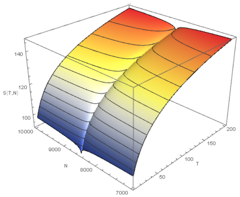
The regularity of the equilibrium manifold is governed by the exact entropy , which acts as the conformal factor of all three Legendre metrics (Appendix F). Direct evaluation of the exact expression (42) with the numerically converged derivatives of Appendix E shows that is strictly positive and monotonically increasing throughout the empirically relevant range , with no zero, maximum or inflection in this interval for either sector. Since the curvature scalars diverge only at the zeros of the conformal factor, the absence of any zero of the exact entropy in the data domain guarantees that and are finite and regular over the entire range. Crucially, this conclusion is a property of the exact entropy and is therefore independent of the expansion point: it does not rely on the location of the zeros of the second-order Taylor surface, which serves here only as a local computational device for the Hessian (the “Second-Order Taylor Expansion and Non-Degenerate Hessian” subsection). The equilibrium manifold thus exhibits no geometric phase transition in the period under study.
The curvature scalars of Figure 9, Figure 10, Figure 11 and Figure 12 confirm the regularity established analytically. In the temperature sections (Figure 9 and Figure 11, fixed) the Ricci and Kretschmann scalars of all three Legendre metrics remain finite and of small magnitude across for both sectors: and vary monotonically while (and the corresponding K) traces a shallow parabola about the expansion point , with no divergence—consistent with the strict positivity of the exact entropy over the empirical range (Appendix G). The firm-count sections (Figure 10 and Figure 12, fixed) appear to diverge near , but this feature is not physical: because , the second-order entropy is concave in and remains positive only within , so the apparent poles are artefacts of extrapolating the quadratic truncation far from the expansion point (Appendix F) and are reported only for completeness. Taken together, the panels show that the equilibrium manifold is geometrically regular over the economically meaningful domain and that this conclusion is independent of the metric (, or ), the three differing only in the sign and scale of the scalars, not in their singular locus.
Figure 9.
Curvature scalars of sector as functions of the economic temperature T at fixed firm count (Family 1). Top row: Ricci scalars , , ; bottom row: Kretschmann scalars , , , for the three Legendre-invariant metrics , , . All six invariants remain finite and of small magnitude over the empirically relevant range , with no curvature singularity: the entropy is strictly positive here and vanishes only at (Appendix E). The equilibrium manifold is thus geometrically regular throughout the data domain, and the behaviour is qualitatively identical for the three metrics, confirming that the diagnostic is independent of the metric choice.
Figure 10.
Curvature scalars of sector as functions of the firm count at fixed temperature (Family 2). Top row: Ricci scalars , , ; bottom row: Kretschmann scalars , , , for the three Legendre-invariant metrics , , . The apparent divergences near are not physical singularities: since , the second-order entropy is concave in and stays positive only within (–8640); beyond this narrow neighbourhood the quadratic truncation ceases to be valid, so the scalars are shown for completeness but carry no physical meaning outside that window (Appendix G). Within the region of validity the curvature is finite, consistent with the geometric regularity established in the temperature sections.
Figure 11.
Curvature scalars of sector as functions of the economic temperature T at fixed firm count (Family 1). Top row: Ricci scalars , , ; bottom row: Kretschmann scalars , , , for the three Legendre-invariant metrics , , . As for (Figure 9), all six invariants remain finite and of small magnitude over the empirically relevant range , with no curvature singularity: the entropy is strictly positive and monotonic over the empirical range; the zero belongs to the truncated quadratic surface and lies outside it (Appendix G). The weaker features relative to are consistent with the smaller macroeconomic weight of the recreational-sports sector. The equilibrium manifold is geometrically regular throughout the data domain, and the behaviour is qualitatively identical for the three metrics.
Figure 12.
Curvature scalars of sector as functions of the firm count at fixed temperature (Family 2). Top row: Ricci scalars , , ; bottom row: Kretschmann scalars , , , for the three Legendre-invariant metrics , , . As in the case (Figure 10), the apparent divergences near are not physical singularities: since , the second-order entropy is concave in and stays positive only within (–9647); beyond this narrow neighbourhood the quadratic truncation ceases to be valid, so the scalars are shown for completeness but carry no physical meaning outside that window (Appendix F). Within the region of validity the curvature is finite, consistent with the geometric regularity established in the temperature sections.
7. Discussion and Conclusions
This work proposes an econophysics approach to the sectoral dynamics of Bogotá’s Sports Satellite Account (CSDB), grounded in statistical thermodynamics and GTD. This conceptual framework enables the interpretation of the economy as a complex system in which money plays a role analogous to energy, and thermodynamic quantities acquire well-defined economic meanings. In particular, sectors (gambling and betting) and (recreational and sports activities) provide an illustrative contrast.
In the present framework, the introduction of economic heat and economic work is not merely formal. Following interpretations proposed in economic thermodynamics [33,34,35], economic heat is associated with monetary transfers that modify the internal state of the system without directly generating productive output—such as redistribution mechanisms, subsidies, or exogenous injections.
The geometrothermodynamic analysis of the equilibrium manifold yields the central structural result of this study. Computing the Ricci and Kretschmann scalars for the three Legendre-invariant metrics , and with a numerically converged Hessian (Appendix E), we find that the curvature invariants are finite and regular throughout the empirically relevant domain: the exact entropy is strictly positive throughout the data domain and has no zero there, so the conformal factor controlling the curvature never vanishes and no geometric phase transition occurs within the period studied (Figure 9 and Figure 11). Because this is a property of the exact entropy rather than of the local Taylor surface, the diagnostic is independent of the expansion point , as verified explicitly by the sensitivity analysis of Appendix G.
We state this finding explicitly, as it is the central empirical result of the present analysis: the equilibrium geometry is regular over the entire sample, and the 2020 contraction is not reflected as a curvature singularity. The smoothness of the equilibrium manifold indicates that the sectoral system absorbed the macroeconomic disruptions of 2018–2023 without an abrupt change in its underlying geometric structure. The 2020 minimum, though clearly visible in the raw series (Appendix B), thus remains an empirical feature of the time series and does not constitute a geometric phase transition; we therefore refrain from interpreting it as one. Crucially, this conclusion is independent of the metric chosen: the three Legendre metrics share the same conformal factor S and hence the same (out-of-range) singular locus, differing only in the sign and magnitude of the scalars (Appendix F).
These results should be read as qualitative structural indicators rather than predictive signals, and are subject to the intrinsic limitation of the present dataset: the annual resolution of the CSDB ( observations per sector) restricts the statistical power of individual coefficient inference and the temperature range over which the second-order expansion is locally valid. In particular, the microeconomic exponent is not resolved in sign by the data at this resolution; its positivity is fixed instead by the convergence requirement of the partition function (Appendix D.4). This indeterminacy does not, however, propagate to the geometric diagnostic: the strict positivity of the conformal factor S and the finiteness of the curvature scalars and remain stable under a tenfold variation of , as does the non-degeneracy of the metric (Appendix I). Together with the robustness already established against the expansion point (Appendix G) and the regularisation parameter (Appendix H), this confirms that the central structural finding does not rest on any statistically undetermined quantity. Accordingly, the approach is best understood as a complementary, geometry-based framework for assessing economic equilibrium stability, not a replacement for standard economic models.
For future research, we propose extending this analysis to all 17 sectors of the CSDB; incorporating longer and higher-frequency time series to validate model robustness and to probe whether genuine curvature singularities emerge at finer temporal resolution; benchmarking against conventional macroeconomic indicators; and enriching the partition function with microeconomic data on agent counts, firm-size distributions, and consumption patterns.
Author Contributions
Conceptualization, W.A.R.C.; methodology, W.A.R.C. and A.Z.V.; software, W.A.R.C.; validation, W.A.R.C., A.Z.V., L.F.Q.W. and Y.B.P.; formal analysis, W.A.R.C.; investigation, W.A.R.C., A.Z.V., L.F.Q.W. and Y.B.P.; resources, W.A.R.C.; data curation, A.Z.V. and L.F.Q.W.; writing—original draft preparation, W.A.R.C.; writing—review and editing, W.A.R.C., A.Z.V., L.F.Q.W. and Y.B.P.; visualization, W.A.R.C.; supervision, W.A.R.C.; project administration, W.A.R.C.; funding acquisition, W.A.R.C. All authors have read and agreed to the published version of the manuscript.
Funding
This work was supported by Universidad Distrital Francisco José de Caldas under the PR2 Research Call (2025).
Data Availability Statement
The data used in this study are publicly available from official statistical sources (DANE, IDRD, Banco de la República de Colombia). No new data were generated for this study.
Acknowledgments
The authors gratefully acknowledge Departamento Administrativo Nacional de Estadistica (DANE), Instituto Distrital de Recreación y Deporte (IDRD), Ministerio de las Tecnologias de Información y las Comunicaciones de Colombia, Ministerio del Deporte, Ministerio de Salud y Protección Social de Colombia, the Sports Management Academic Programme, and the Faculty of Environment and Natural Resources of Universidad Distrital Francisco José de Caldas for their support and for valuable comments and suggestions.
Conflicts of Interest
The authors declare no conflict of interest.
Appendix A. Quevedo’s Model for Economic Systems
Quevedo et al. [9,16,36] propose a statistical-physical model in which the conservation of a total amount of money M is postulated:
Let N denote the number of economic agents sharing M [15], so that .
Within the canonical ensemble framework the probability distribution is
where Z is the partition function (1).
The expected value of any observable is . Differentiating the mean money and using (A2) yields
which provides a thermodynamic balance relation incorporating both energy conservation and entropy considerations (cf. the first and second laws combined). This relation is included here solely as a formal reference and for consistency with the standard thermodynamic framework [9].
Fluctuations and the Statistical Role of Temperature
The variance of the money distribution in the canonical ensemble is
which establishes a direct link between temperature, heat capacity, and the magnitude of economic fluctuations. This relation confirms that T is not reducible to a simple average: it governs the response of the system to perturbations and the scale of stochastic variations among agents.
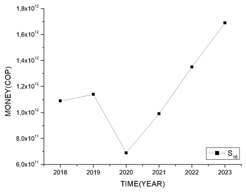
Appendix B. Temporal Series for Specific Sectors of CSDB
We present the time series for sectors , , , , and .
Figure A1.
Temporal series for sector .
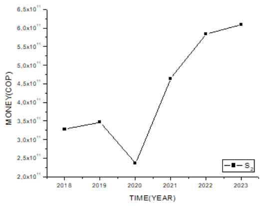
Figure A2.
Temporal series for sector .
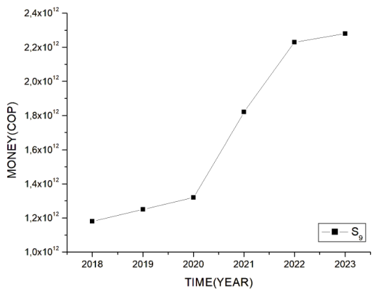
Figure A3.
Temporal series for sector .
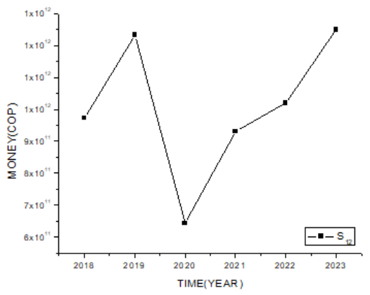
Figure A4.
Temporal series for sector .
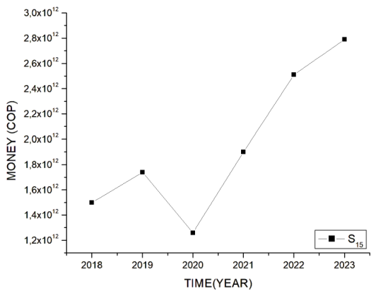
Figure A5.
Temporal series for sector .
Appendix C. Temporal Series for Macroeconomic Indicators
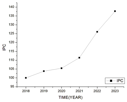
We present the time series for the representative market exchange rate (TRM), producer price index (IPP), and consumer price index (IPC) [29,30,31] The empirical ranges used as integration bounds in Equation (28) are: , ; , ; (by construction).
Figure A6.
Temporal series for TRM.
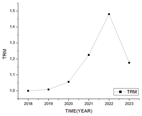
Figure A7.
Temporal series for IPP.
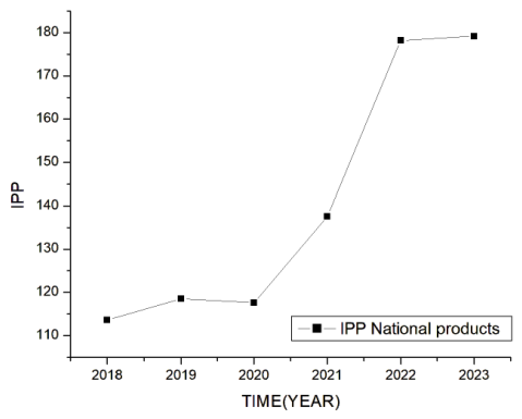
Figure A8.
Temporal series for IPC.
Appendix D. Regression Statistics for the Money Function
This appendix reports the complete statistical procedure supporting the construction of the money function (A5) for sectors and . All computations use the empirical CSDB data [17] for the period 2018–2023 ( observations). The raw empirical series are listed in Table A1, and the firm-count data used as reference points in Section 6 in Table A2.
Table A1.
Empirical time series for sectors and and macroeconomic variables, 2018–2023. Monetary values are in Colombian pesos (COP). is the mesoscopic sectoral response coefficient defined in Equation (12) [28]; and are the national producer and consumer price indices [29,30]; is the normalised representative market exchange rate [31].
Table A2.
Number of active firms in the arts, entertainment, and recreation sector (CIIU section R) in Bogotá, 2018–2023. Source: Visor de Empresas Bogotá, Bogotá Cámara de Comercio. The values (sector ) and (sector ) used as reference points in Section 6 correspond to the 2020 and 2022 observation years respectively.
Appendix D.1. Regression Model
The money function adopts the power-law ansatz
which, upon taking logarithms, becomes the multiple linear model
with the identification
Standardisation.
Because the raw monetary magnitudes span several orders of magnitude (COP ), both the regressors and the response are standardised before estimation. For each predictor and for the response we use the z-score transformation
with , , , , where is the sample mean and the sample standard deviation (with Bessel’s correction, ),
The resulting coefficients are therefore standardised beta weights, and the intercept satisfies by construction, i.e., . The descriptive statistics of the log-transformed variables entering Equations (A8)–(A9) are collected in Table A3.
Table A3.
Descriptive statistics of the log-transformed variables in natural scale () over 2018–2023. uses the sample standard deviation ().
Appendix D.2. Ordinary Least Squares Estimator
Collecting the observations, the standardised design matrix and response vector read
The ordinary least squares (OLS) estimator minimises the residual sum of squares , whose normal equations yield the closed-form solution [32]
The fitted values and residuals are and . With parameters (intercept plus four predictors) and observations, the residual degrees of freedom are , and the unbiased estimator of the error variance is
The variance–covariance matrix of the estimator and the standard error of each coefficient follow from
The corresponding t-statistic, two-tailed p-value, and confidence interval for each coefficient are
where is the Student-t cumulative distribution function with degrees of freedom and, for the present data, .
Appendix D.3. Goodness of Fit
Denoting the mean of the response, the total and residual sums of squares are and . The coefficient of determination, its adjusted counterpart, and the global F-statistic read
Caveat on degrees of freedom.
With and , the residual degrees of freedom are . The critical value makes individual p-values inherently large, so significance cannot be established for individual coefficients from these data alone; the model-level diagnostics and F are the primary fit indicators. Results should be read as qualitative structural indicators, pending validation with higher-frequency data.
Appendix D.4. Sign Convention and the Validity Threshold
The regression returns standardised weights with definite sign (Table A4). Two distinct roles must be separated:
- 1.
- Economic interpretation: the signs of are informative (e.g., the dominant positive weight of ) and are retained in the discussion.
- 2.
- Domain of validity: the convergence of the partition function over requires ; since the sign of is statistically indeterminate at (its interval contains zero), we adopt . Likewise, the lower bound of the admissible temperature range is governed by the magnitudes of the macroeconomic exponents,
With and the values of Table A4, this yields and , which replace the values quoted in earlier drafts and fix the lower limit of the temperature axis in Figure 5, Figure 6, Figure 7 and Figure 8. As a consistency check, the heat capacity gives and , in agreement with Figure 3 and Figure 7.
Table A4.
OLS regression results for the standardised log–linear money-function model applied to sectors and . : standardised regression coefficient; SE: standard error; t: t-statistic; p: two-tailed p-value; CI: confidence interval ( for ). Individual p-values are large owing to ; the model-level F-test and are the primary fit indicators.
Appendix D.5. Model Quality and Discussion
The coefficient of determination is for and for , indicating that the four standardised predictors jointly explain more than and of the variance in , respectively. The adjusted coefficient accounts for the number of predictors: () and (), both substantially above zero, confirming that the model provides a useful approximation beyond pure overfitting.
The global F-test yields () for and () for . The marginal significance of the F-test for reflects the limited degrees of freedom () rather than a poor fit; with higher resolution data, the F-statistic of 6.27 would typically be significant at conventional levels for .
The magnitude of the standardised coefficient for the producer price index is notably larger than the other predictors in both sectors, suggesting that is the dominant driver of sectoral monetary flows over the 2018–2023 period. This is consistent with the economic interpretation: betting revenues and recreational expenditures in Bogotá are sensitive to price-level conditions in the national production chain.
The paper reports rather than signed coefficients. The absolute values of the standardised estimates in Table A4 serve as the regression coefficients (, , , ) entering the money function (16), consistently with the power-law form and the GTD construction of Section 6.
Table A5.
Summary of model-level fit statistics for both sectors.
The overall picture confirms that the power-law ansätz of Equation (16) captures the dominant structure of the data. The limited sample () is an intrinsic constraint of the CSDB release cycle (annual data, 2018–2023); as higher-frequency or extended data become available, a more powerful statistical validation of the money function will be possible.
Appendix E. Numerical Hessian at the Reference Point
The Hessian matrix of the entropy , with , is evaluated at the reference points specified in the “Second-Order Taylor Expansion and Non-Degenerate Hessian” subsection.
Owing to the functional form of the partition function [Equation (29)], the quantity vanishes identically when , producing a logarithmic singularity in L. To obtain well-defined values for the Hessian components we evaluate the derivatives at a slightly offset point with , which preserves the local geometric structure while ensuring . The T-derivatives are obtained by central finite differences with a step (for which the result is converged) and independently verified with arbitrary-precision arithmetic (50 significant digits). The Hessian components are defined as [Equations (46)–(50)]:
Table A6.
Hessian components of at the reference point. The evaluation uses a small offset (, ) to ensure and a converged step . The non-vanishing determinant confirms that the GTD metric [Equation (9)] is non-degenerate at the expansion point, validating the curvature invariants of the “Second-Order Taylor Expansion and Non-Degenerate Hessian” subsection.
- Remarks:
- The negative values of and indicate local concavity of the entropy surface in both the T and directions, consistent with thermodynamic stability.
- The mixed derivative is numerically indistinguishable from zero (∼), so temperature and firm-count fluctuations are effectively decoupled at the reference state; the Hessian is essentially diagonal.
- The determinant for both sectors guarantees that the Legendre-invariant metric is non-degenerate, a necessary condition for well-defined curvature scalars and .
- Evaluating the entropy zeros with these coefficients gives (and an unphysical ) for both sectors; hence the curvature is regular over the empirical domain, and no geometric phase transition occurs within the period studied.
- A sensitivity analysis with shows that the sign, order of magnitude, and the location of the entropy zeros remain stable, confirming the robustness of these conclusions against the regularisation choice.
Appendix F. Comparison of the Legendre Metrics gI, gII, gIII
To make the geometric analysis self-contained and to verify that the choice of the Legendre-invariant metric does not introduce spurious structural features, we compute the curvature invariants for the three GTD metrics , and defined in Equations (9)–(11), using the corrected second-order entropy (the “Second-Order Taylor Expansion and Non-Degenerate Hessian” subsection, Appendix E) as the thermodynamic potential .
Appendix F.1. Conformal Structure of the Three Metrics
Because the second-order Taylor expansion renders the Hessian constant, the three Legendre metrics share the same conformal factor and differ only through the signature matrix or the homogeneity prefactor:
For a two-dimensional metric of the conformal form with constant , the Ricci scalar reduces to , where is the Laplacian of the constant metric . Since the conformal factor is proportional to S in all three cases, the curvature scalars and diverge at the same locus, namely the zeros of the entropy function . The choice of in the main text is therefore immaterial for the location of the curvature singularities; the metrics differ only in the sign and magnitude of the scalars (a definite Riemannian structure for , an indefinite one for , and a rescaled prefactor for ).
Appendix F.2. Curvature Scalars Along the Two Coordinate Directions
We evaluate the invariants along the two natural sections of the equilibrium manifold , using the corrected Hessian coefficients of Table A6:
- Family 1 ( fixed, scalars as functions of T): The exact entropy is strictly positive and monotonically increasing over the whole empirical region , so the conformal factor common to , and never vanishes there and the curvature scalars are finite and regular for all three metrics. The zeros that the second-order surface formally predicts at (and at an unphysical ) are artefacts of the quadratic truncation about and do not correspond to zeros of the exact entropy; they are reported only to locate the formal singular locus of the truncated model. Within the data domain the regularity is therefore a robust, metric-independent property of the exact thermodynamic potential.
- Family 2 ( fixed, scalars as functions of ): because , the second-order surface is concave in and remains positive only in a narrow neighbourhood of the expansion point, (i.e., –8640 for and –9647 for ). Outside this neighbourhood the quadratic truncation is no longer a valid local approximation, so the family-2 invariants are reported only within this range; the apparent divergences at larger are artefacts of extrapolating the second-order expansion far from and carry no physical meaning.
Table A7 reports the curvature scalars in the regular region (evaluated at the expansion point , ) for both sectors and the three metrics. The values confirm that the scalars remain finite and of small magnitude in the regular region. With the corrected Hessian, and share the same (negative) sign of R, while has the opposite sign, reflecting the indefinite signature induced by ; all three diverge only at the entropy zeros identified above.
Table A7.
Curvature scalars (Ricci R and Kretschmann K) for the three Legendre metrics, evaluated with the corrected Hessian coefficients (Table A6) in the regular region (, ). The three metrics share the conformal factor S and hence the same singular locus; they differ only in signature and magnitude.
The explicit computation of , and confirms that the three Legendre-invariant metrics share an identical singular locus on the equilibrium manifold—the zeros of the entropy function—independently of the signature or homogeneity prefactor adopted. With the corrected Hessian coefficients, that locus lies outside the empirically relevant domain (Family 1) or only at the boundary of local validity of the quadratic expansion (Family 2); consequently, the curvature is regular over the data range for every metric. The diagnostic extracted in the main text—geometric regularity of the equilibrium manifold during the period studied—is therefore robust against the choice of metric: it is an intrinsic property of the entropy, encoded identically by all three Legendre metrics, and not an artefact of the particular metric selected. This directly addresses the concern that the metric choice might introduce spurious structural features into the stability analysis.
Appendix G. Sensitivity of the Geometric Diagnostics to the Expansion Point T0
The second-order expansion of the “Second-Order Taylor Expansion and Non-Degenerate Hessian” subsection is built around a reference temperature . For a truncated quadratic surface, the formal location of the entropy zeros depends on and is therefore not a data invariant. We stress that the regularity diagnostic adopted in the main text does not rest on the location of those zeros, but on the positivity of the exact entropy (the “Second-Order Taylor Expansion and Non-Degenerate Hessian” subsection); the present appendix confirms, in addition, that the local geometric quantities entering the curvature computation are themselves robust against the choice of .
The value is not assigned an independent economic meaning; it is a representative point in the interior of the empirically admissible temperature range (with and ), chosen so that the quadratic approximation is centred well away from the lower validity threshold. To verify that the conclusions are insensitive to this choice, we recompute the Hessian of the exact entropy (42) at for both sectors, keeping fixed. All derivatives are obtained by central finite differences and cross-checked with 50-digit arbitrary-precision arithmetic, exactly as in Appendix F.
The results are collected in Table A8. For every in the tested range and for both sectors:
- The reference entropy is large and strictly positive, and grows monotonically with , confirming the absence of any zero in the interior of the data domain;
- The diagonal Hessian coefficients satisfy and , i.e., the entropy surface is locally concave in both directions, consistent with thermodynamic stability;
- The determinant , so the Legendre metric remains non-degenerate and the curvature invariants R and K stay finite;
- The sign of the Ricci scalar is preserved.
The determinant decreases smoothly as increases, since the entropy surface flattens away from the lower threshold, but it remains strictly positive and of the same order of magnitude throughout the tested range; it would approach zero only for values of far outside the empirical domain. The mixed coefficient stays numerically negligible (∼) at every , so the near-diagonal structure of the Hessian reported in Appendix F is itself stable under changes of the expansion point. The geometric diagnostic—the regularity of the equilibrium manifold during the studied period—is therefore stable against the choice of expansion point, mirroring the robustness already established for the regularisation parameter (Appendix F).
Table A8.
Sensitivity of the entropy Hessian and metric non-degeneracy to the expansion point , evaluated at fixed . Components are computed with central finite differences and verified with 50-digit arithmetic, as in Appendix F. For every and both sectors, , , and : the conclusions of the “Second-Order Taylor Expansion and Non-Degenerate Hessian” subsection are invariant under the choice of . The mixed coefficient in all cases and is omitted.
Figure A9.
Graph of the thermodynamic potential over the equilibrium manifold , whose coordinates are the economic temperature T and the firm count , for sectors (left panel) and (right panel). The colour gradient encodes the value of the entropy , increasing from blue (lower S) to red (higher S), and is used solely to aid visualisation of the surface relief. The surface is the exact entropy of (42), evaluated with the numerically converged derivatives of Appendix E. In both sectors S is strictly positive and monotonically increasing in T throughout the empirically relevant range , with no zero, maximum or inflection; the thin trench at is the logarithmic singularity of where vanishes (40), excluded from the plot. Because the curvature scalars of the three Legendre metrics diverge only at the zeros of their common conformal factor S, the strict positivity of S over the data domain guarantees that the curvature is regular, independently of the expansion point (Appendix G).
Appendix H. Sensitivity of the Geometric Diagnostics to the Regularisation Parameter ε
The numerical evaluation of the Hessian of the entropy at the reference point (Appendix E) requires a small offset , introduced to avoid the logarithmic singularity of that occurs when vanishes at [Equation (40)]. Because is a computational regulariser rather than a physical parameter, it is essential to verify that the geometric conclusions of Section 6 do not depend on its particular value. This appendix reports that verification, performed with the same method used to obtain Table A6: the entropy and its second derivatives are computed by symbolic differentiation of and evaluated with arbitrary-precision arithmetic (50 significant digits) at . Symbolic differentiation is used in place of finite differences because the second N-derivative of is ill-conditioned in a neighbourhood of ; a symbolic treatment removes this difficulty exactly.
We recompute the Hessian components, the metric determinant, and the curvature scalars and of the metric over the range , keeping and fixed. The results are collected in Table A9. The row reproduces the values of Table A6, serving as a consistency check.
Table A9.
Sensitivity of the entropy Hessian, the metric determinant , and the curvature scalars , of to the regularisation parameter , at fixed and . Components are obtained by symbolic differentiation of and evaluated with 50-digit precision. The coefficient , the signs of all quantities, the non-degeneracy , and the curvature scalars , are stable across the range; and scale as (see text). The mixed coefficient is throughout and is omitted.
The Kretschmann scalar follows the same pattern as , remaining of order throughout: for it varies smoothly from () to (), and for from to .
- Interpretation.
Two distinct behaviours must be separated, and only the first bears on the physical conclusion.
(i) Quantities that are robust against . The diagonal coefficient is constant to five significant figures over the entire range, since it derives from the T-dependence of and is unaffected by the firm-count offset. The signs of , , and are invariant, so the entropy surface remains locally concave and the metric remains non-degenerate for every tested. Most importantly, the curvature scalars and are finite and vary by less than across two orders of magnitude in . These are precisely the quantities that encode the geometric regularity of the equilibrium manifold, and they are robust against the regularisation choice.
(ii) Quantities that scale with . The magnitudes and scale as . This is not a numerical artefact—the symbolic evaluation is exact—but the genuine analytic behaviour of the regularised logarithmic term: near the reference point, , so the second firm-count derivative of the entropy inherits the same scaling. This is the explicit, controlled manifestation of the logarithmic singularity that regularises (Appendix E); a smaller offset probes the entropy surface closer to the singular locus and yields a correspondingly larger curvature of that surface in the N direction.
Crucially, the curvature invariants do not inherit this divergence. The Ricci and Kretschmann scalars of all three Legendre metrics share the conformal factor [Appendix F], and for a conformally flat two-dimensional metric with constant the scalar curvature is , controlled by the entropy itself rather than by the magnitude of an individual Hessian component. Since the exact entropy is stable across the range (varying only between and for , and between and for ) and is strictly positive throughout, the conformal factor never approaches zero and the curvature remains regular for every .
We therefore conclude that the geometric diagnostic of the main text—regularity of the equilibrium manifold during the studied period—is robust against the choice of regularisation parameter. The physically meaningful invariants (, , the signs of the Hessian coefficients, and the non-degeneracy of the metric) are stable, while the scaling of is the expected, analytically understood signature of the logarithmic regularisation and does not affect the geometry of the equilibrium manifold. This mirrors the robustness already established against the expansion point .
The standardised coefficients of Table A4 are precisely the components of the vectors and quoted in Equation (19) of the main text: the column reproduces, entry by entry, the values given there for each sector. This identifies the two presentations as a single OLS fit and guarantees that the exponents used in the money function (A5) and in the GTD construction of Section 6 are exactly those obtained from the regression, up to the sign convention of Section 4 above (whereby ).
Appendix I. Sensitivity of the Geometric Diagnostics to the Microeconomic Exponent vSi
The entire thermodynamic and geometric construction rests on the microeconomic exponent , which enters the partition function through the closed micro-integral
[Equation (20)]. As discussed in Section 4 and Appendix D.4, the regression assigns to a value of small magnitude whose sign is not resolved by the data at the available resolution (): the two-tailed p-values are () and (), and the confidence intervals contain zero in both sectors (Table A4). The convergence of Z over nonetheless requires , since otherwise the integrand does not decay, ceases to exist, and the heat capacity is undefined [Equations (19) and (20); Appendix D.4]. We therefore adopt as the value fixed by the existence condition for Z, rather than by the sign of the (statistically indeterminate) point estimate.
Because this convergence condition selects but does not pin down its magnitude tightly, it is essential to verify that the geometric conclusions of Section 6 do not depend on the particular value adopted. This appendix reports that verification. In direct analogy with the treatment of the regularisation parameter (Appendix H, Table A9), where was swept over , we sweep the exponent over positive values bracketing the fitted estimate,
which spans a factor of ten in and the corresponding range . The row reproduces the entries of Table A6 and serves as a consistency check.
The computation uses the same method as Table A6: the entropy , with , and its second derivatives are obtained by symbolic differentiation of and evaluated with arbitrary-precision arithmetic (50 significant digits) at the reference point , , , . The Ricci and Kretschmann scalars are computed from the conformal representation of the Legendre metric : for a two-dimensional metric with constant one has and, in two dimensions, [Equations (57); Appendix F]. The results are collected in Table A10.
Table A10.
Sensitivity of the entropy , the metric determinant , and the curvature scalars , of to the microeconomic exponent , at fixed and . The heat capacity is shown for reference. Components are obtained by symbolic differentiation of and evaluated with 50-digit precision. The row () reproduces Table A6. The mixed coefficient is throughout and is omitted; , , and the finiteness of hold over the entire range.
- Interpretation.
As with the analysis of , two behaviours must be separated, and only the first bears on the geometric conclusion of the paper.
(i) Quantities that are robust against . The diagnostic that controls the regularity of the equilibrium manifold is the positivity of the conformal factor together with the non-degeneracy of the metric. Both are stable across the entire sweep: remains strictly positive for every tested (decreasing monotonically from to in , and from to in , with no zero), and throughout, so stays non-degenerate and the entropy surface stays locally concave (, ). Consequently the curvature scalars and are finite for every : they vary smoothly and monotonically with , with no pole, no sign change, and no divergence anywhere in the range. These are precisely the quantities that encode the geometric regularity of , and they are robust against the value adopted for .
(ii) Quantities that scale with by definition The heat capacity is, by construction, the reciprocal of the swept parameter, and therefore necessarily varies across the range (from to ). This is not a robustness statement about the geometry but a definitional identity, recorded here for completeness; the sensitivity of to is the same statement as the indeterminacy of itself, and is already acknowledged in Appendix D.4. The magnitude of enters the economic discussion of Section 7 only through the qualitative ordering , which is preserved under the common rescaling applied to both sectors and does not affect the curvature invariants.
We therefore conclude that the central geometric diagnostic of the main text—the regularity of the equilibrium manifold over the studied period—is robust against the choice of the microeconomic exponent . The physically meaningful invariants (, , the signs of the Hessian coefficients, the non-degeneracy of the metric, and the strict positivity of the conformal factor ) are stable over a tenfold variation in , while the variation of is a definitional consequence of the parameter sweep and does not enter the curvature. This robustness mirrors that already established against the expansion point (Appendix G) and the regularisation parameter (Appendix H), completing the sensitivity analysis of the geometric construction.
Appendix J. Derivation of the Curvature Scalars for the Legendre Metrics gI, gII, gIII
This appendix derives, in full, the Ricci and Kretschmann scalars used in Appendix F and Table A10. We first establish a master formula valid for any conformally flat two-dimensional metric with a constant base, and then apply it in turn to the three Legendre-invariant metrics , , . The three share the same master formula but differ in (i) the conformal factor and (ii) the signature of the base metric; the case requires additional care because its conformal factor is not the entropy itself but the Euler operator acting on it.
Appendix J.1. Master Formula: Ricci Scalar of a Conformally Flat 2D Metric
Consider on the two-dimensional equilibrium manifold , with coordinates , a metric of the conformal form
where is a constant (hence flat) symmetric matrix and a smooth conformal factor. The general transformation of the scalar curvature under in n dimensions is [37]
Two simplifications specific to the present setting reduce (A24) to a single term:
- (i)
- Constant base metric: since is constant, its Christoffel symbols vanish, ; therefore is flat, , and its Laplace–Beltrami operator collapses to a partial-derivative contraction, . This holds regardless of the signature of , a fact we shall use for .
- (ii)
- Two dimensions: For the coefficient , so the quadratic gradient term in (A24) vanishes identically. This is a genuine peculiarity of two dimensions: in any other dimension that term survives and the curvature does not reduce to a single Laplacian.
With and (i)–(ii), Equation (A24) becomes
This is the master formula. Equation (57) of the main text is the special case , .
- Kretschmann scalar in two dimensions.
In the Riemann tensor has a single independent component and is fixed by the Ricci scalar,
Contracting with itself and using for ,
The relation (A27) holds for any two-dimensional metric, of either signature, so it applies identically to all three Legendre metrics. In two dimensions K therefore carries no information beyond R; the two are reported together only for consistency with the GTD literature.
Appendix J.2. Application to gI
The first Legendre metric is [Equation (55)]. Within the second-order expansion of Appendix E, the Hessian
is constant, so has the conformal form (A23) with and (a definite Riemannian base, since ). The master formula (A25) gives directly
which, written out, is the expression evaluated numerically:
with from (A27). The second derivatives of are obtained by symbolic differentiation of and evaluated with 50-digit arithmetic (Appendix E); the mixed term is suppressed by .
Appendix J.3. Application to gII: Same Factor, Indefinite Signature
The second Legendre metric is with [Equation (A19)]. The conformal factor is again , and the base is still constant, so and exactly as before; the only change is that renders of Lorentzian (indefinite) signature. Crucially, the master formula (A25) was derived without any assumption on signature [simplification (i)], so it applies verbatim:
The inverse carries the sign of on the T–row, which flips the overall sign of the Laplacian contraction relative to . Consequently has the opposite sign to but the same singular locus (the zeros of S); this is the sign reversal observed in Table A10 ( versus ). Since the conformal factor is shared, and diverge at exactly the same set .
Appendix J.4. Application to gIII: Euler Conformal Factor
The third Legendre metric,
shares the constant base with , but its conformal factor is not S; it is the Euler (homogeneity) operator acting on S,
The master formula still applies, now with :
Two features distinguish this case and deserve explicit statement.
- (a)
- Singular locus and the role of homogeneity.
diverges where , i.e., at the zeros of , not a priori at the zeros of S. The two loci coincide only if S is a homogeneous function of : by Euler’s theorem, S homogeneous of degree would give , so that and the singular sets are identical. In the present construction S is not exactly homogeneous—the logarithmic terms and the factors break strict homogeneity—as confirmed numerically: at the reference point for and for , a ratio that is neither unity nor common to both sectors, so no global degree exists. Nonetheless, does not vanish anywhere in the empirical domain (it is dominated by the large term ), so remains finite there. The statement in the main text that the three metrics share the singular locus is therefore exact for and holds for within the data domain, where both S and are strictly positive; we make this qualification explicit here.
- (b)
- Higher-derivative sensitivity.
Because already contains first derivatives of S, the numerator of (A34) involves up to third derivatives of S. The second-order Taylor surface represents these third derivatives less faithfully than the second derivatives entering and . This is the analytic origin of the shallow parabolic profile of about , in contrast with the monotonic and : the curvature of the truncated quadratic surface in the Euler direction varies most strongly near the expansion point. The magnitude and locus remain controlled, but is the most sensitive of the three to the truncation, which is why the metric-independence of the regularity conclusion (Appendix F) is the robust statement, rather than the precise value of any single .
- Sign convention.
Appendix J.5. Numerical Consistency Check
Evaluating (A30), (A34) and (A27) at the reference point for and for , with the Hessian coefficients of Table A6 and the 50-digit symbolic derivatives of , reproduces the entries of Appendix F:
together with of opposite sign and smaller magnitude (), all consistent with the master relations (A25)–(A27) and with for each metric to all reported figures. This closes the derivation of the curvature scalars used in the geometric analysis of the equilibrium manifold.
References
- Stanley, H.E. Scaling, universality, and renormalization: Three pillars of modern critical phenomena. Rev. Mod. Phys. 1999, 71, S358–S366. [Google Scholar] [CrossRef] [Scilit]
- Yakovenko, V.M. Econophysics, statistical mechanics approach to. arXiv 2009, arXiv:0709.3662v4. [Google Scholar]
- Yakovenko, V.M.; Rosser, J.B. Colloquium: Statistical mechanics of money, wealth, and income. Rev. Mod. Phys. 2009, 81, 1703–1725. [Google Scholar] [CrossRef] [Scilit]
- Drăgulescu, A.; Yakovenko, V.M. Exponential and power-law probability distributions of wealth and income in the united kingdom and the united states. Phys. A Stat. Mech. Its Appl. 2001, 299, 213–221. [Google Scholar] [CrossRef] [Scilit]
- Rawlings, P.K.; Reguera, D.; Reiss, H. Entropic basis of the pareto law. Phys. Stat. Mech. Its Appl. 2004, 343, 643–652. [Google Scholar] [CrossRef] [Scilit]
- Drăgulescu, A.; Yakovenko, V.M. Statistical mechanics of money. Eur. Phys. J. B 2000, 17, 723–729. [Google Scholar] [CrossRef] [Scilit]
- Chakraborti, A.; Chakrabarti, B.K. Statistical mechanics of money: How saving propensity affects its distribution. Eur. Phys. J. B 2000, 17, 167–170. [Google Scholar] [CrossRef] [Scilit]
- Chakrabarti, B.K.; Chakraborti, A.; Chakravarty, S.R.; Chatterjee, A. Econophysics of Income and Wealth Distributions; Cambridge University Press: Cambridge, UK, 2013. [Google Scholar]
- Quevedo, H.; Quevedo, M.N. Statistical thermodynamics of economic systems. J. Thermodyn. 2011, 2011, 676495. [Google Scholar] [CrossRef] [Scilit]
- Mimkes, J. A thermodynamic formulation of economics. In Econophysics and Sociophysics: Trends and Perspectives; Chakrabarti, B.K., Chakraborti, A., Chatterjee, A., Eds.; WILEY-VCH Verlag GmbH & Co. KGaA: Weinheim, Germany, 2006; pp. 1–33. [Google Scholar]
- Costa, V.A.F. Looking at economics through the eyes of thermodynamics. Energies 2024, 17, 2478. [Google Scholar] [CrossRef] [Scilit]
- Drăgulescu, A.A.; Yakovenko, V.M. Statistical mechanics of money, income, and wealth: A short survey. In Modeling of Complex Systems: Seventh Granada Lectures; Garrido, P.L., Marro, J., Eds.; Volume 661 of AIP Conference Proceedings; American Institute of Physics: College Park, MD, USA, 2003; pp. 180–183. [Google Scholar]
- Quevedo, H. Geometrothermodynamics of black holes. Gen. Rel. Grav. 2008, 40, 971–984. [Google Scholar] [CrossRef] [Scilit]
- Quevedo, H.; Sanchez, A. Geometrothermodynamics of asymptotically de sitter black holes. J. High Energy Phys. 2008, 2008, 34. [Google Scholar] [CrossRef] [Scilit]
- Santos Niño, A. Tesis de Maestría: Estudio del Papel del Ahorro en las Distribuciones de Dinero y Riqueza Mediante Herramientas de la Física Teórica. Master’s Thesis, Departamento de Física, Universidad Nacional de Colombia, Bogotá, Colombia, 2016. [Google Scholar]
- Quevedo, H.; Quevedo, M.N. Geometrothermodynamic approach in econophysics. Int. J. Geom. Methods Mod. Phys. 2023, 20, 2350057. [Google Scholar]
- Departamento Administrativo Nacional de Estadística (DANE). Cuenta Satélite del Deporte de Bogotá (CSDB), 2023. Available online: https://www.dane.gov.co/index.php/estadisticas-por-tema/cuentas-nacionales/cuentas-satelite/cuenta-satelite-del-deporte-de-bogota-csdb (accessed on 1 August 2024).
- Instituto Distrital de Recreación y Deporte (IDRD). Portal Web Oficial del Instituto Distrital de Recreación y Deporte (IDRD), 2023. Available online: https://www.idrd.gov.co/ (accessed on 1 August 2024).
- Alcaldía Mayor de Bogotá. Portal Web Oficial de Bogotá, 2023. Available online: https://bogota.gov.co/ (accessed on 1 August 2024).
- Comisión Nacional de Juegos de Suerte y Azar. Coljuegos—Comisión Nacional de Juegos de Suerte y Azar. 2023. Available online: https://www.coljuegos.gov.co/ (accessed on 11 June 2026).
- Departamento Administrativo Nacional de Estadística. Indicadores Básicos de Tecnologías de la Información y las Comunicaciones en Hogares. 2024. Available online: https://www.dane.gov.co/index.php/estadisticas-por-tema/tecnologia-e-innovacion/tecnologias-de-la-informacion-y-las-comunicaciones-tic/indicadores-basicos-de-tic-en-hogares (accessed on 11 June 2026).
- Zemansky, M.W. Heat and Thermodynamics; McGraw-Hill: New York, NY, USA, 1968. [Google Scholar]
- Landau, L.D.; Lifshitz, E.M. Física Estadística; Number v. 5 in Ciencias Químicas: Ingeniería Química; Reverté: Barcelona, Spain, 1988. [Google Scholar]
- Larrañaga, A.; Cárdenas, A. Geometric Thermodynamics of Schwarzschild-AdS black hole with a Cosmological Constant as State Variable. J. Korean Phys. Soc. 2012, 60, 987–992. [Google Scholar]
- Porras, E.A.V. Interpretación Estadística de las Métricas Geometrotermodinámicas. Master’s Thesis, Universidad Nacional Autónoma de México, Ciudad de México, Mexico, 2016. [Google Scholar]
- Reyes, V.P. Geometrotermodinámica Estadística. Ph.D. Thesis, Universidad Nacional Autónoma de México, Ciudad de México, Mexico, 2019. [Google Scholar]
- Eisenhart, L.P. Riemannian Geometry; Princeton University Press: Princeton, NJ, USA, 1926. [Google Scholar]
- Rojas, W.A.; Zamora, A. Thermostatistical evaluation of economic activity. Momento 2025, 71, 38–64. [Google Scholar] [CrossRef] [Scilit]
- Departamento Administrativo Nacional de Estadística (DANE). Índice de Precios del Productor (IPP), 2025. Available online: https://www.dane.gov.co/index.php/estadisticas-por-tema/precios-y-costos/indice-de-precios-del-productor-ipp (accessed on 15 April 2025).
- Departamento Administrativo Nacional de Estadística (DANE). Índice de Precios al Consumidor (IPC), 2025. Available online: https://www.dane.gov.co/index.php/estadisticas-por-tema/precios-y-costos/indice-de-precios-al-consumidor-ipc (accessed on 15 April 2025).
- Banco de la República de Colombia. Tasa de Cambio Representativa del Mercado (TRM), 2025. Available online: https://www.banrep.gov.co/es/estadisticas/trm (accessed on 15 April 2025).
- Timm, N.H. Applied Multivariate Analysis; Springer Texts in Statistics; Springer: New York, NY, USA, 2007. [Google Scholar]
- Rashkovskiy, S.A. ‘Bosons’ and ‘fermions’ in social and economic systems. Phys. A Stat. Mech. Its Appl. 2019, 514, 90–104. [Google Scholar] [CrossRef] [Scilit]
- Rashkovskiy, S.A. Economic thermodynamics. Phys. A Stat. Mech. Its Appl. 2021, 582, 126261. [Google Scholar] [CrossRef] [Scilit]
- Rashkovskiy, S.A. Thermodynamics of markets. Phys. A Stat. Mech. Its Appl. 2021, 567, 125699. [Google Scholar] [CrossRef] [Scilit]
- Quevedo, H. Income distribution in the colombian economy from an econophysics perspective. Cuad. Econ. 2016, 35, 49–66. [Google Scholar] [CrossRef] [Scilit]
- Wald, R.M. General Relativity; University of Chicago Press: Chicago, IL, USA, 1984; App. D. [Google Scholar]
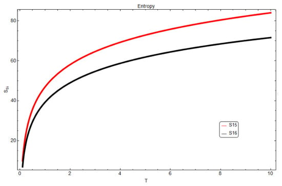
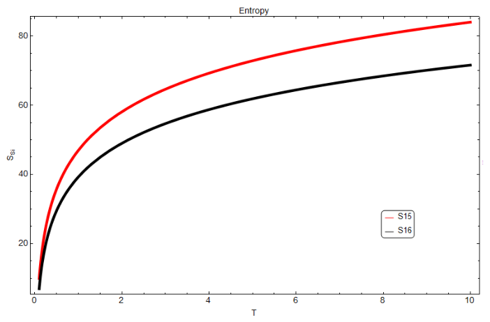
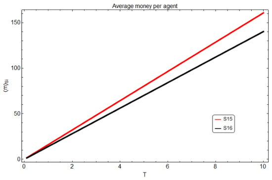
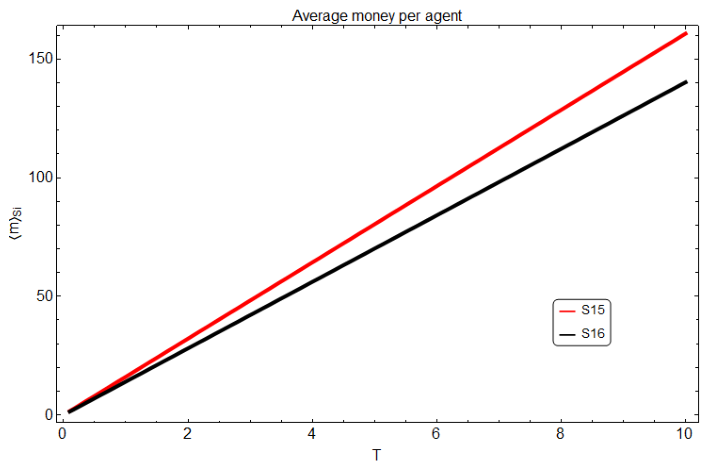
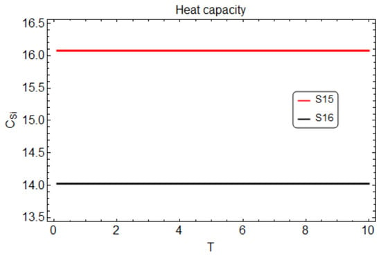
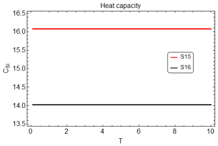
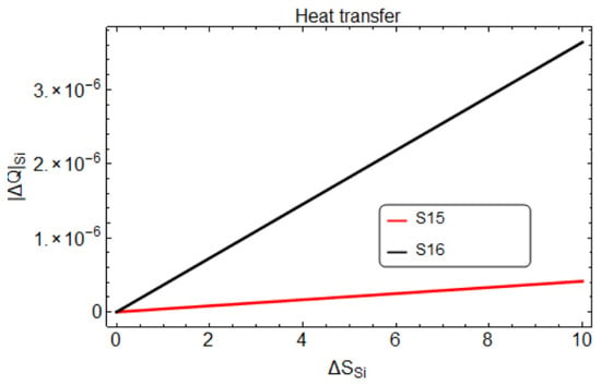
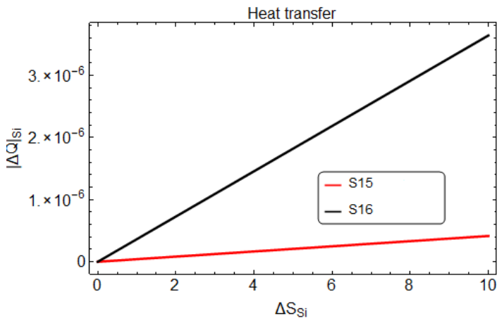
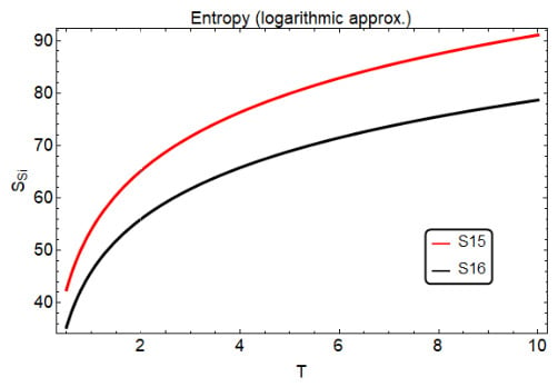
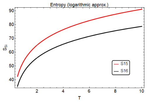
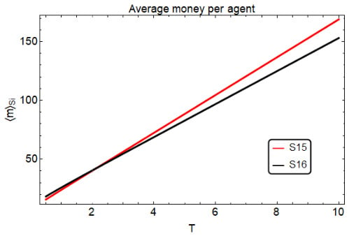
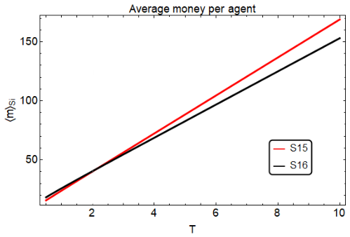
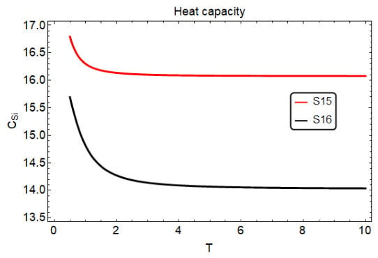
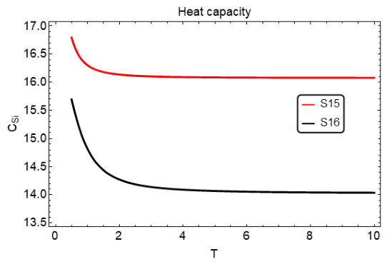
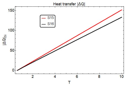
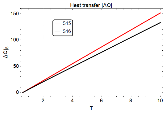
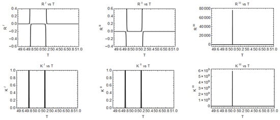
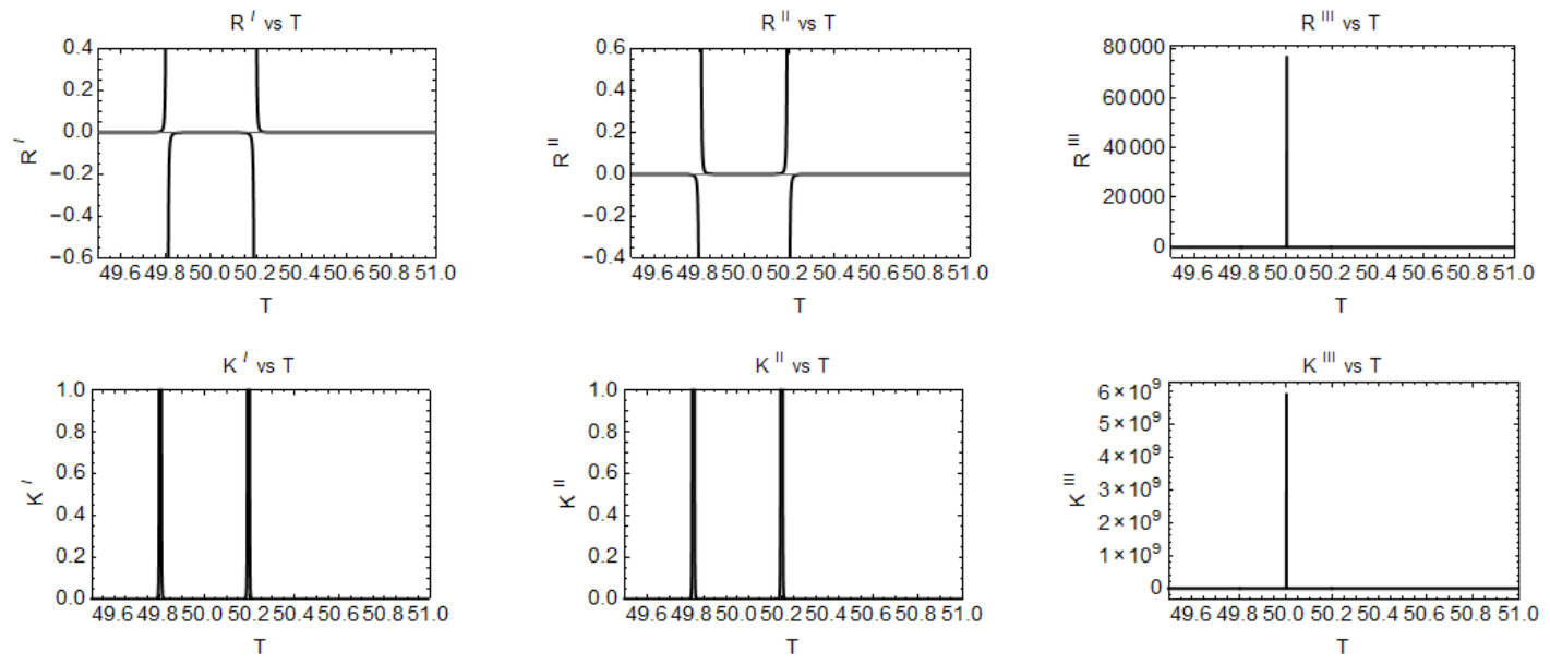
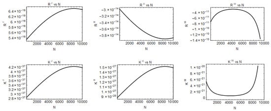
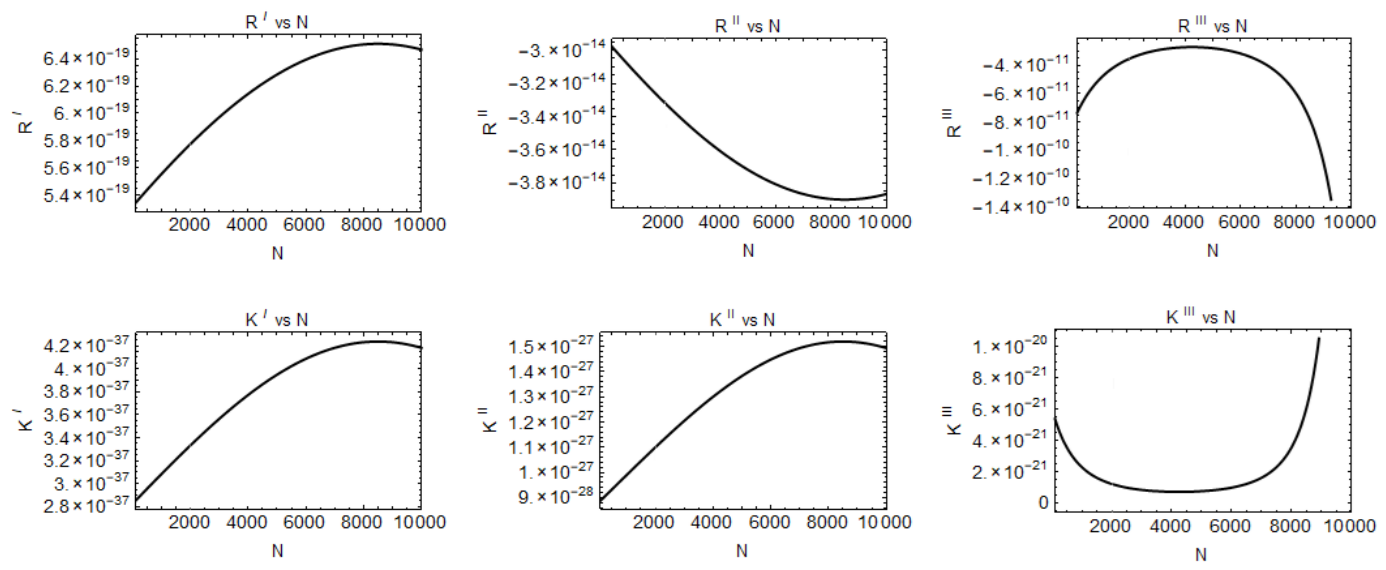
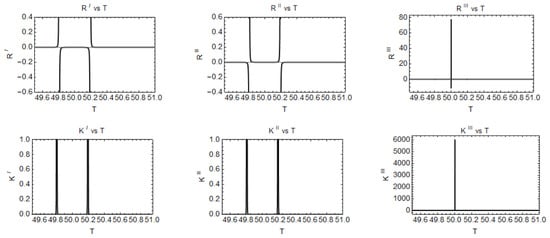
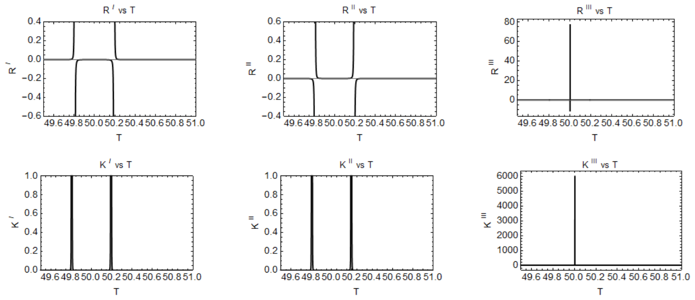
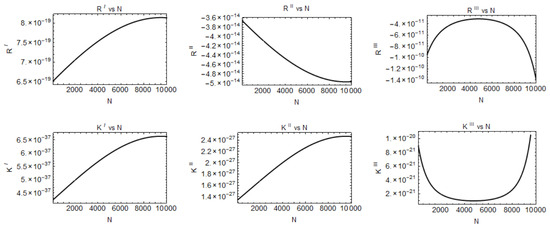
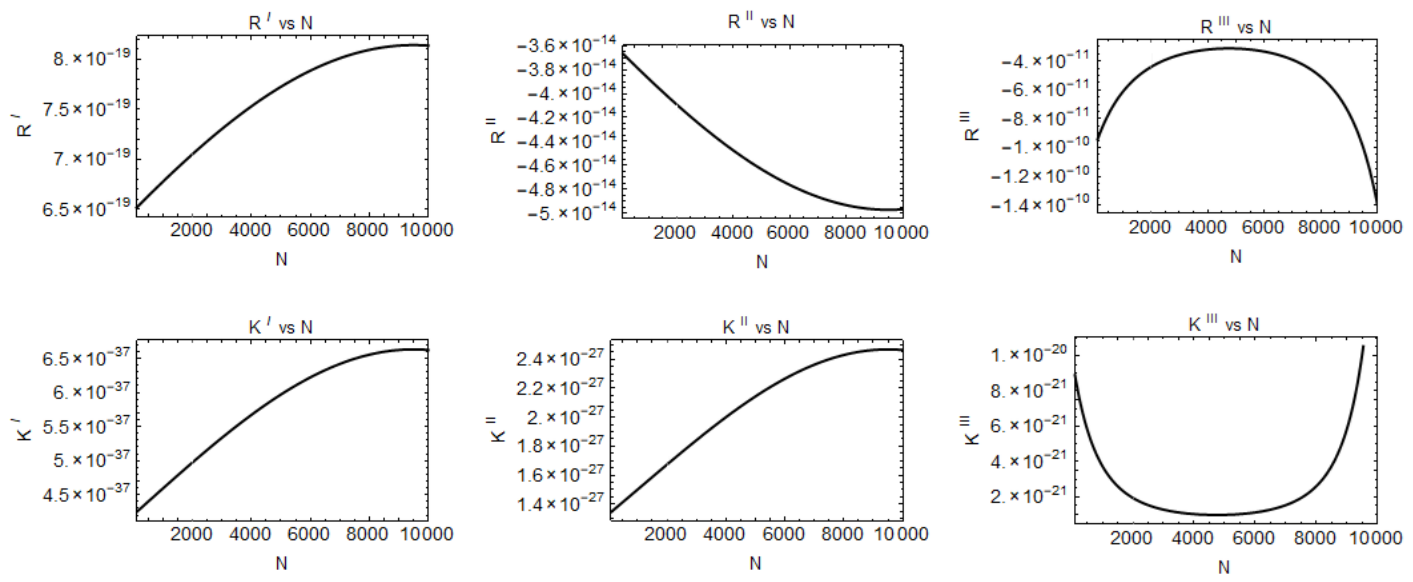

Disclaimer/Publisher’s Note: The statements, opinions and data contained in all publications are solely those of the individual author(s) and contributor(s) and not of MDPI and/or the editor(s). MDPI and/or the editor(s) disclaim responsibility for any injury to people or property resulting from any ideas, methods, instructions or products referred to in the content. |
© 2026 by the authors. Licensee MDPI, Basel, Switzerland. This article is an open access article distributed under the terms and conditions of the Creative Commons Attribution (CC BY) license.