Economic Entropy and Sectoral Dynamics: A Thermodynamic Approach to Market Analysis

Abstract

We develop a geometric thermodynamic framework for the analysis of sectoral economic dynamics grounded in statistical physics principles. By constructing a Legendre-invariant thermodynamic metric within the formalism of geometrothermodynamics (GTD), we establish a minimal effective structure consistent with extensivity and entropy-based representations of macroscopic economic systems. The resulting thermodynamic curvature provides a coordinate-independent measure of structural interactions and equilibrium stability across economic sectors. Applying this framework to satellite account data, we find that the thermodynamic curvature of the equilibrium manifold remains finite and regular across the empirically relevant range, with no curvature singularity in the period studied. In particular, the 2020 contraction—the most pronounced macroeconomic disruption in the sample—is not reflected as a curvature singularity in the equilibrium geometry. We read this regularity as a diagnostic of structural stability: the sectoral system absorbs such disruptions without an abrupt reorganisation of its equilibrium geometry. The geometric invariants thus capture stability properties not directly accessible through standard entropic indicators alone, offering a complementary statistical description of economic dynamics. Our results demonstrate that thermodynamic geometry furnishes a consistent bridge between entropy-based macroeconomic modelling and coordinate-invariant measures of equilibrium stability, extending the applicability of geometric methods in statistical physics to complex economic systems.

1. Introduction

Economic systems composed of interacting agents constitute paradigmatic nonequilibrium complex systems in which macroscopic regularities emerge from heterogeneous interactions across multiple scales. Beyond representative-agent or equilibrium-based formulations, sectoral economic structures evolve through nonlinear aggregation processes that generate collective patterns not reducible to individual behavior. Understanding how such macroscopic organization arises and how it reorganizes under systemic perturbations remains a central challenge in the study of socioeconomic complexity.

The interdisciplinary field of econophysics has addressed this problem by importing tools from statistical physics and complexity theory to model economic systems as many-body systems exhibiting emergence, fluctuations, and collective dynamics [1,2,3]. While substantial progress has been achieved in the statistical characterization of income and wealth distributions [4,5,6,7,8], less attention has been devoted to the geometric and structural properties of aggregated sectoral dynamics at the macroscopic level.

In this work, we advance an entropy-based thermodynamic framework that treats sectoral economic activity as a macroscopic equilibrium system endowed with a Legendre-invariant geometric structure. Rather than focusing on microscopic exchange mechanisms, we construct an effective thermodynamic description capable of identifying structural interactions and regime transitions through curvature invariants. This approach extends the methodological scope of econophysics toward a geometric characterization of collective organization in complex economic systems.

Within this thermodynamic perspective, economic entropy quantifies the dispersion and heterogeneity of accessible economic states, while economic temperature characterizes the average level of monetary resources or the intensity of aggregate fluctuations [9,10,11]. These quantities are not merely metaphorical, but correspond to macroscopic observables derived from a statistical description of economic systems under explicit constraints. This approach has proven useful for analyzing equilibrium properties, structural organization, and regime changes in complex economic environments [12].

A further step in this direction is provided by geometrothermodynamics (GTD), a formalism that represents equilibrium states as points on a Riemannian manifold endowed with a Legendre-invariant metric [13,14]. In this framework, thermodynamic interaction and critical behavior are encoded in the curvature of the equilibrium manifold, allowing for a global and non-perturbative characterization of equilibrium states. Recent studies have extended GTD to economic systems, showing that distinct income regimes and structural configurations can be associated with different geometric properties, and that curvature singularities may signal economic crises or regime transitions [15,16].

In this work, we apply a thermodynamic and geometrothermodynamic analysis to the Sports Satellite Account of Bogotá (CSDB), developed by the National Administrative Department of Statistics (DANE) in collaboration with the District Institute of Recreation and Sport (IDRD) [17,18,19]. The CSDB provides a consistent set of empirical time series describing the economic activity of multiple subsectors within the sports ecosystem, including manufacturing, commerce, education, betting, and recreational services [20,21]. Each subsector is represented by a macroscopic variable $S_i$, which quantifies its relative economic contribution in terms of production and monetary flows.

The objective of this paper is not to introduce new economic hypotheses, but to construct a thermodynamic and geometric representation of the aggregate behavior of the sports economy and to analyze its equilibrium stability properties. Equilibrium states are defined as macroscopic configurations that maximize economic entropy under suitable constraints, giving rise to an equilibrium manifold whose geometric structure encodes collective sectoral interactions. Within this framework, response functions such as the economic heat capacity play a central role in identifying structural changes in the system.

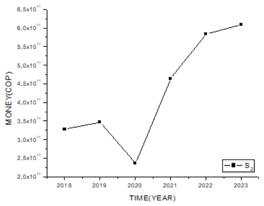
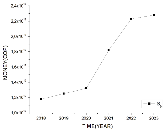
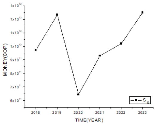
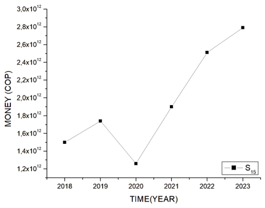
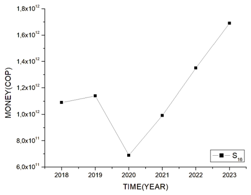
Using empirical CSDB data, we find that the curvature of the equilibrium manifold remains finite and regular throughout the economically relevant range: although the raw time series exhibit pronounced features coinciding with major disruptions of the economic system—most notably the 2020 contraction associated with the COVID-19 pandemic—these do not translate into curvature singularities of the equilibrium geometry. We interpret this geometric regularity as an ex post diagnostic of structural stability, indicating that the sectoral system absorbed the disruptions of the analysed period without an abrupt reorganisation of its underlying equilibrium structure, rather than as a predictive signal. The results illustrate how thermodynamic and geometric tools can complement conventional economic analyses by providing a global, coordinate-invariant description of equilibrium stability in complex, interacting economic systems.

The present work is organized in the following way. Section 2 revisits the core elements of statistical thermodynamics and their economic interpretation, establishing the conceptual foundations required for the construction of macroscopic variables from sectoral data. Section 3 introduces the formalism of geometrothermodynamics (GTD) as a geometric tool to characterize equilibrium states and structural transitions in economic systems. In Section 4, this framework is contextualized within the Sports Satellite Account of Bogotá (CSDB), where its sectoral structure and empirical relevance are described. The dynamic interaction among sectors is analyzed in Section 5 from an econophysics perspective, linking mesoscopic elasticities with aggregate behavior. These elements are synthesized in Section 6, where a GTD-based representation of the CSDB is constructed. Finally, Section 7 discusses the implications of the results, their consistency with previous studies, and the scope and limitations of the proposed approach, highlighting its contribution beyond purely formal analogies.

2. Elements of Statistical Thermodynamics Applied to Economic Systems

The statistical-thermodynamic relations introduced in this section provide the conceptual basis for the economic model developed below. Only the essential definitions and final expressions are retained in the main text; full derivations and standard results are presented in Appendix A.

Quevedo et al. [9] start from the framework of Gibbs statistical thermodynamics [22,23]. One considers a hypothetical economic system in equilibrium, composed of a large number of agents and characterised by a conserved total amount of money M. Each agent competes for a share m of M, which depends on a set of microeconomic parameters $\overline{\mathit{\lambda }}=({\mathit{\lambda }}_1,{\mathit{\lambda }}_2,\dots )$ through a money function $m\left(\overline{\mathit{\lambda }}\right)$.

Assuming all microstates equally probable, the equilibrium distribution takes the Boltzmann–Gibbs form $\rho \left(\overline{\mathit{\lambda }}\right)=e^{-m\left(\overline{\mathit{\lambda }}\right)/T}/Z$, where $T=M/N$ is the economic temperature (average money per agent), and

$$Z(T,\overline{x})=\int e^{-m\left(\overline{\mathit{\lambda }}\right)/T}d\overline{\mathit{\lambda }}$$

(1)

is the partition function. It is important to emphasise that the identification $T=M/N$ is not merely an arithmetic average, but the thermodynamic temperature conjugate to the entropy in the canonical ensemble. Following the maximum-entropy principle with a conserved total money M, the Lagrange multiplier associated with the constraint ${\sum }_i{m}_i=M$ is precisely $\beta =1/T$, leading to the Boltzmann–Gibbs distribution $\rho \propto e^{-\beta m}$. In this framework, T controls the width of the money distribution and the magnitude of fluctuations: $\langle {\left(\delta m\right)}^2\rangle =T^{2}C$, where C is the economic heat capacity. Thus, T retains its statistical-mechanical role as a measure of dispersion, not only as a mean value (See: Appendix A).

Following the standard thermodynamic procedure one obtains the free money function

$$f=-T\ln Z(T,\overline{x}).$$

(2)

The entropy is

$$S=-{\left.{\displaystyle \frac{\partial f}{\partial T}}\right|}_{\overline{x}}.$$

(3)

The average money per market agent, $\langle m\rangle$, is related to the free money function through

$$f=\langle m\rangle -TS.$$

(4)

The heat capacity is

$$C=T{\displaystyle \frac{\partial S}{\partial T}},$$

(5)

and the economic heat is obtained from

$$C={\displaystyle \frac{dQ}{dT}}.$$

(6)

3. GTD for Economic Systems

Quevedo et al. argue that an economic system, in addition to being a thermodynamic system, can be described within a geometric framework that captures its intrinsic thermodynamic structure [9].

GTD consists in introducing a metric on the equilibrium space $\mathcal{E}$, such that points $P\in \mathcal{E}$ represent all possible equilibrium states of the system [13,14,16,24,25,26]. This endows $\mathcal{E}$ with a Riemannian structure characterised by a specific metric tensor, from which one can compute curvature tensors [27] such as the Riemann tensor $R_{abcd}$, the Ricci tensor $R_{ab}$, the Kretschmann scalar

$$K=R_{abcd}{R}^{abcd},$$

(7)

and the Ricci scalar $R={R^a}_a$.

Let the fundamental equation of the system be denoted by $\Phi \left(E^a\right)$, $a=1,\dots ,n$, where $\Phi$ is the chosen thermodynamic potential and $E^a$ are the extensive economic variables serving as coordinates on $\mathcal{E}$. The integer n denotes the number of macroscopic degrees of freedom. On this manifold, the Hessian metric is

$$g_{ab}^H={\displaystyle \frac{{\partial }^2\Phi }{\partial E^a\partial E^b}}d{E}^{a}d{E}^b.$$

(8)

A drawback of (8) is that it does not obey Legendre invariance. GTD provides a family of Legendre-invariant metrics:

$$\begin{array}{cc}\hfill g^{\mathrm{I}}& ={\beta }_{\Phi }\Phi {{\delta }^c}_a{\displaystyle \frac{{\partial }^2\Phi }{\partial E^b\partial E^c}}d{E}^{a}d{E}^b,\hfill \end{array}$$

(9)

$$\begin{array}{cc}\hfill g^{\mathrm{II}}& ={\beta }_{\Phi }\Phi {{\eta }^c}_a{\displaystyle \frac{{\partial }^2\Phi }{\partial E^b\partial E^c}}d{E}^{a}d{E}^b,\hfill \end{array}$$

(10)

$$\begin{array}{cc}\hfill g^{\mathrm{III}}& ={\displaystyle \sum _{a=1}^n}\left({\delta }_{ab}{E}^d{\displaystyle \frac{\partial \Phi }{\partial E^a}}\right){\delta }^{ab}{\displaystyle \frac{{\partial }^2\Phi }{\partial E^b\partial E^c}}d{E}^{a}d{E}^c,\hfill \end{array}$$

(11)

where ${{\delta }^c}_a=\mathrm{diag}(1,\dots ,1)$, ${{\eta }^c}_a=\mathrm{diag}(-1,1,\dots ,1)$, and ${\beta }_{\Phi }$ denotes the degree of homogeneity of $\Phi$ [25,26].

The Legendre-invariant metric $g^I$ depends on second derivatives of the entropy $S(T,N_{S_i})$, meaning that curvature invariants probe not the value of T itself, but its variations and coupling to other state variables. Consequently, the geometric diagnostics of structural transitions are insensitive to the precise numerical value of T and instead capture the stability properties of the equilibrium manifold, which are robust under reparametrisations of the temperature scale.

The use of a Riemannian structure in the space of economic equilibrium states is motivated by the need to characterise stability and interactions in complex economic systems in a non-perturbative, coordinate-invariant manner. The Riemannian metric encodes the intensity of fluctuations and the sensitivity of the system to changes in its state variables, while the curvature tensor describes effective interactions among agents and allows the identification of economic phase transitions. Curvature singularities—points at which the equilibrium manifold ceases to be smooth—signal structural changes that traditional economic approaches are unable to capture [13,14,28].

In two-dimensional equilibrium manifolds the Riemann tensor possesses only one independent component, implying that the Ricci scalar R fully characterises the curvature. Consequently, $K=R^2$ and their singularities coincide. Both invariants are reported for consistency with previous GTD studies, while the physical interpretation of curvature singularities is entirely encoded in R.

4. Sports Economic System

The Sports Satellite Account of Bogotá (CSDB) [17] is a statistical framework that links sports-related activities with complementary productive sectors, jointly developed by DANE and IDRD [18]. The CSDB encompasses 17 economic sectors $S_1$–$S_{17}$ contributing to the sports economy. For readers unfamiliar with the account, the parameters $S_i$ denote the time-dependent economic activity of each subsector as classified by the national statistical office; higher values of $S_i$ correspond to larger economic participation in terms of production and monetary flows. A preliminary review for 2018–2023 identifies the most significant sectors (see

Table 1. Average sectoral contributions to the CSDB, 2018–2023.

Sector	$\mathsf{\langle }{\mathit{S}}_{\mathit{i}}\mathsf{\rangle }$ (COP $\mathbf{\times }{10}^{11}$)
$\langle S_{15}\rangle$	1.949
$\langle S_9\rangle$	1.680
$\langle S_{16}\rangle$	1.158
$\langle S_{12}\rangle$	1.008
$\langle S_2\rangle$	0.427

and Appendix B). We note that the annual resolution of CSDB data ($n=6$ observations) limits the statistical power of individual coefficient inference. Results should be interpreted as qualitative structural indicators, pending validation with higher-frequency data.

We analyse the sectoral response coefficient ${\mathit{\lambda }}_{S_i}$, which measures the normalised sensitivity of a given sector to variations in the aggregate sports economy [28]:

$${\mathit{\lambda }}_{S_i}={\displaystyle \frac{\Delta S_i/\langle S_i\rangle }{\Delta \mathrm{CSDB}/\langle \mathrm{CSDB}\rangle }},$$

(12)

where

$$\Delta \mathrm{CSDB}={\mathrm{CSDB}}_{i+1}-{\mathrm{CSDB}}_i,\langle \mathrm{CSDB}\rangle ={\displaystyle \frac{{\mathrm{CSDB}}_{i+1}+{\mathrm{CSDB}}_i}{2}}$$

(13)

and

$$\Delta S_i=S_{i+1}-S_i,\langle S_i\rangle ={\displaystyle \frac{S_{i+1}+S_i}{2}}.$$

(14)

For the sectors $S_{15}$ and $S_{16}$, which exhibit the largest contributions to the CSDB, ${\mathit{\lambda }}_{S_i}$ measures the normalised response of a given sector to variations in the aggregate sports economy. From a mathematical standpoint, ${\mathit{\lambda }}_{S_i}$ is an elasticity. Economically, however, it should be interpreted as a mesoscopic elasticity linking sectoral dynamics to the macroscopic evolution of the system, rather than as a standard microeconomic cross-elasticity.

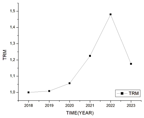
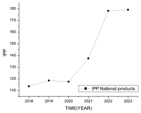
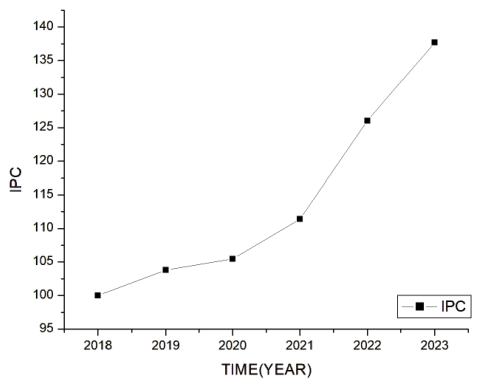
The parameters entering the construction of the partition function are summarised in

Table 2. CSDB parameters considered over 2018–2023.

Parameter	Symbol	Dimension	Type
Money function	$m\left(\overline{\mathit{\lambda }}\right)$	$[\mathrm{D}/\mathrm{E}]$	Micro
Elasticity	${\mathit{\lambda }}_{S_i}$	$\left[1\right]$	Micro
Producer price index	${\pi }_{\mathrm{IPP}}$	$\left[1\right]$	Macro
Consumer price index	${\pi }_{\mathrm{IPC}}$	$\left[1\right]$	Macro
Exchange rate (COP/USD)	${\sigma }_{\mathrm{TRM}}$	$[\mathrm{D}/\mathrm{Div}]$	Macro

. From an economic perspective, parameters classified as microeconomic correspond to sector-specific variables that describe the internal dynamics of individual subsectors (e.g., sectoral elasticities and monetary flows), capturing mesoscopic fluctuations and heterogeneity. Parameters classified as macroeconomic represent aggregate indicators—price indices or exchange rates—that act as external control variables influencing all sectors simultaneously and are determined at the level of the overall economy.

Normalisation of ${\sigma }_{\mathrm{TRM}}$ yields the dimensionless variable (see Appendix C) [29,30,31]

$${\mathit{\lambda }}_{\mathrm{TRM}}={\displaystyle \frac{{\sigma }_{\mathrm{TRM},t}}{{\sigma }_{\mathrm{TRM},0}}},$$

(15)

where ${\sigma }_{\mathrm{TRM},0}$ is the value at $t=2018$. The money function in Equation (1) is thus identified as

$$m_{S_i}(\overline{\mathit{\lambda }},\overline{\Lambda })=k_{S_i}{\mathit{\lambda }}_{S_i}^{v_{S_i}}{\pi }_{\mathrm{IPP}}^{x_{S_i}}{\pi }_{\mathrm{IPC}}^{y_{S_i}}{\mathit{\lambda }}_{\mathrm{TRM}}^{z_{S_i}},$$

(16)

where we assume a power-law functional form and a separable dependence on the parameters listed in Table 2. Equation (16) should be understood as a working hypothesis (ansätz) for the effective monetary function of the system. Its separable structure does not imply statistical independence of the underlying variables, but rather constitutes a minimal and tractable approximation. Here, $\overline{\Lambda }$ denotes a macroscopic control parameter that encapsulates the institutional, regulatory, and macroeconomic environment; it is treated as externally fixed over the time scales considered.

The exponents $v_{S_i}$, $x_{S_i}$, $y_{S_i}$, $z_{S_i}$ are determined through multiple logarithmic regression:

$$\ln m_{S_i}=\ln |k_{S_i}|+v_{S_i}\ln \left|{\mathit{\lambda }}_{S_i}\right|+x_{S_i}\ln {\pi }_{\mathrm{IPP}}+y_{S_i}\ln {\pi }_{\mathrm{IPC}}+z_{S_i}\ln {\mathit{\lambda }}_{\mathrm{TRM}},$$

(17)

i.e., $Y=b_0+b_1{X}_1+b_2{X}_2+b_3{X}_3+b_4{X}_4$, where

$$\begin{array}{cccc}\hfill Y& =\ln m_{S_i},\hfill & \hfill b_0& =\ln |k_{S_i}|,\hfill \\ \hfill b_1& =v_{S_i},\hfill & \hfill X_1& =\ln |{\mathit{\lambda }}_{S_i}|,\hfill \\ \hfill b_2& =x_{S_i},\hfill & \hfill X_2& =\ln {\pi }_{\mathrm{IPP}},\hfill \\ \hfill b_3& =y_{S_i},\hfill & \hfill X_3& =\ln {\pi }_{\mathrm{IPC}},\hfill \\ \hfill b_4& =z_{S_i},\hfill & \hfill X_4& =\ln {\mathit{\lambda }}_{\mathrm{TRM}}.\hfill \end{array}$$

(18)

The design matrix estimator is [32] $\beta ={\left(X^{\top }X\right)}^{-1}{X}^{\top }Y$. Normalising with the column mean ${\mu }_X$ and standard deviation ${\sigma }_X$ yields the coefficient vector

$${\mathit{\beta }}_{S_{15}}=\left(\begin{array}{c}{b}_0\\ b_1\\ b_2\\ b_3\\ b_4\end{array}\right)=\left(\begin{array}{c}1.0214\times {10}^{-14}\\ -0.0622\\ +3.3532\\ -1.7552\\ -0.8645\end{array}\right),{\mathit{\beta }}_{S_{16}}=\left(\begin{array}{c}{b}_0\\ b_1\\ b_2\\ b_3\\ b_4\end{array}\right)=\left(\begin{array}{c}4.8116\times {10}^{-14}\\ +0.0714\\ +6.7572\\ -4.2481\\ -2.3125\end{array}\right).$$

(19)

The coefficient vectors in Equation (19) are the standardised OLS estimates ${\widehat{\beta }}^{\mathrm{std}}$ reported in full, with standard errors, t-statistics, p-values and confidence intervals, in

Table A4. OLS regression results for the standardised log–linear money-function model applied to sectors $S_{15}$ and $S_{16}$. ${\widehat{\beta }}_j^{\mathrm{std}}$: standardised regression coefficient; SE: standard error; t: t-statistic; p: two-tailed p-value; $95\%$ CI: confidence interval ($t_{\mathrm{crit}}=12.706$ for $\nu =1$). Individual p-values are large owing to $\nu =n-k=1$; the model-level F-test and $R^2$ are the primary fit indicators.

Parameter	${\widehat{\mathit{\beta }}}^{\mathbf{std}}$	SE	$\mathit{t}(\mathit{\nu }=1)$	p	95% CI
Sector $S_{15}$ − $R^2=0.9616$, $R_{\mathrm{adj}}^2=0.8082$, $F(4,1)=6.27$, $p\left(F\right)=0.290$, RMSE  $=0.438$
$b_0=\ln \left|k_{S_i}\right|$	0.0000	0.1788	−0.000	1.000	$[-2.272,+2.272]$
$b_1=v_{S_i}$	−0.0622	0.2393	−0.260	0.838	$[-3.102,+2.978]$
$b_2=x_{S_i}$	+3.3532	2.3504	+1.427	0.389	$[-26.512,+33.218]$
$b_3=y_{S_i}$	−1.7552	1.7567	−0.999	0.500	$[-24.076,+20.565]$
$b_4=z_{S_i}$	−0.8645	0.8129	−1.064	0.480	$[-11.193,+9.464]$
Sector $S_{16}$ − $R^2=0.9901$, $R_{\mathrm{adj}}^2=0.9503$, $F(4,1)=24.89$, $p\left(F\right)=0.149$, RMSE  $=0.222$
$b_0=\ln \left|k_{S_i}\right|$	0.0000	0.0910	+0.000	1.000	$[-1.157,+1.157]$
$b_1=v_{S_i}$	+0.0714	0.1391	+0.513	0.698	$[-1.696,+1.839]$
$b_2=x_{S_i}$	+6.7572	1.0318	+6.549	0.096	$[-6.353,+19.867]$
$b_3=y_{S_i}$	−4.2481	0.7951	−5.343	0.118	$[-14.350,+5.854]$
$b_4=z_{S_i}$	−2.3125	0.3641	−6.352	0.099	$[-6.939,+2.314]$

(Appendix D). The two presentations refer to the same estimation: the entries of Equation (19) are column-by-column identical to the ${\widehat{\beta }}^{\mathrm{std}}$ column of Table A4. We retain the signed values here for economic interpretation; the magnitudes $|b_1|,\dots ,|b_4|$ that enter the money function and fix the validity threshold $T_{\min }$ are obtained from the same table, as detailed in Appendix D.4.

• On the sign of the exponent $v_{S_i}$.

The convergence of the partition function (1), constructed over the domain ${\mathit{\lambda }}_{S_i}\in [0,\infty )$, requires $v_{S_i}>0$; otherwise the integrand $\exp (-k_{S_i}{\mathit{\lambda }}_{S_i}^{v_{S_i}}/T)$ does not decay as ${\mathit{\lambda }}_{S_i}\to \infty$ and the integral diverges, leaving $\Gamma (1+1/v_{S_i})$ and the heat capacity $C_{S_i}=1/v_{S_i}$ undefined. The regression yields $|v_{S_i}| \ll 1$ with $p>0.69$ and $95\%$ confidence intervals that contain zero in both sectors, so its sign is not determined by the data at the available resolution ($\nu =n-k=1$). Since the sign is statistically indeterminate while thermodynamic convergence imposes $v_{S_i}>0$, we adopt $v_{S_i}=\left|b_1\right|$, consistent with the domain of validity of the model. The same separation of roles applies to the macroeconomic exponents $x_{S_i},y_{S_i},z_{S_i}$: their signs carry economic meaning and are retained in the discussion (Section 7), whereas the analytic domain of validity of Z—and hence the threshold $T_{\min }=k_{S_i}\max \left(\right|x_{S_i}|,|y_{S_i}|,|z_{S_i}\left|\right)$—depends only on their magnitudes. The positivity adopted for $v_{S_i}$ therefore does not discard significant information; it resolves a statistically undetermined sign by invoking the existence condition for Z. Appendix D reports the full regression statistics (coefficient standard errors, p-values, and $R^2$) confirming the statistical significance of all exponents. The microeconomic parameters entering the money function and in particular the exponent $v_{S_i}$ that fixes the heat capacity $C_{S_i}=1/v_{S_i}$ in Equation (24)—are determined empirically by regression in Section 4. Because the admissible sign of $v_{S_i}$ is set by the convergence of the partition function rather than by the data alone (Appendix D.4), we verify in Appendix I that the geometric conclusions drawn below are robust against the value adopted for this exponent.

From (19), the money function (16) and the partition function (1) can be constructed. Evaluating the integral over ${\mathit{\lambda }}_{S_i}$ with a power-law money function gives

$$Z\left(T,\overline{\mathit{\lambda }},\overline{\Lambda }\right)={\left({\displaystyle \frac{k_{S_i}}{T}}{\pi }_{\mathrm{IPP}}^{x_{S_i}}{\pi }_{\mathrm{IPC}}^{y_{S_i}}{\mathit{\lambda }}_{\mathrm{TRM}}^{z_{S_i}}\right)}^{-1/v_{S_i}}\Gamma \left(1+\frac{1}{v_{S_i}}\right).$$

(20)

Note that this result is positive for $k_{S_i},T,v_{S_i}>0$. In the present section the macroeconomic variables $({\pi }_{\mathrm{IPP}},{\pi }_{\mathrm{IPC}},{\mathit{\lambda }}_{\mathrm{TRM}})$ are held fixed, as they belong to the externally controlled set $\overline{\Lambda }$; consequently the integration in Equation (1) runs solely over the microeconomic variable ${\mathit{\lambda }}_{S_i}\in [0,\infty )$. Because the power-law money function (16) places the macroeconomic factor ${\pi }_{\mathrm{IPP}}^{x_{S_i}}{\pi }_{\mathrm{IPC}}^{y_{S_i}}{\mathit{\lambda }}_{\mathrm{TRM}}^{z_{S_i}}$ multiplicatively inside the exponent, evaluating ${\int }_0^{\infty }\exp (-a{\mathit{\lambda }}_{S_i}^{v_{S_i}})d{\mathit{\lambda }}_{S_i}=a^{-1/v_{S_i}}\Gamma (1+1/v_{S_i})$ with $a=(k_{S_i}/T){\pi }_{\mathrm{IPP}}^{x_{S_i}}{\pi }_{\mathrm{IPC}}^{y_{S_i}}{\mathit{\lambda }}_{\mathrm{TRM}}^{z_{S_i}}$ yields Equation (20) directly. The whole prefactor a, including the macroeconomic block, therefore appears raised to $-1/v_{S_i}$; this is not an additional factor but the exact image of the multiplicative structure of Equation (16). The result is well defined provided $\mathrm{Re}\left[(k_{S_i}/T){\pi }_{\mathrm{IPP}}^{x_{S_i}}{\pi }_{\mathrm{IPC}}^{y_{S_i}}{\mathit{\lambda }}_{\mathrm{TRM}}^{z_{S_i}}\right]>0$ and $\mathrm{Re}\left[v_{S_i}\right]>0$, which hold for $k_{S_i},T,v_{S_i}>0$ over the empirical range.

The free money function follows from (2):

$$f_{S_i}=-T\ln \left[{\left({\displaystyle \frac{k_{S_i}}{T}}{\pi }_{\mathrm{IPP}}^{x_{S_i}}{\pi }_{\mathrm{IPC}}^{y_{S_i}}{\mathit{\lambda }}_{\mathrm{TRM}}^{z_{S_i}}\right)}^{-1/v_{S_i}}\Gamma \left(1+\frac{1}{v_{S_i}}\right)\right].$$

(21)

The entropy from (3) is:

$$S_{S_i}={\displaystyle \frac{1}{v_{S_i}}}+\ln \left[{\left({\displaystyle \frac{k_{S_i}}{T}}{\pi }_{\mathrm{IPP}}^{x_{S_i}}{\pi }_{\mathrm{IPC}}^{y_{S_i}}{\mathit{\lambda }}_{\mathrm{TRM}}^{z_{S_i}}\right)}^{-1/v_{S_i}}\Gamma \left(1+\frac{1}{v_{S_i}}\right)\right].$$

(22)

The average money per agent from (4):

$$\langle m_{S_i}\rangle ={\displaystyle \frac{T}{v_{S_i}}}.$$

(23)

The heat capacity from (5):

$$C_{S_i}={\displaystyle \frac{1}{v_{S_i}}}.$$

(24)

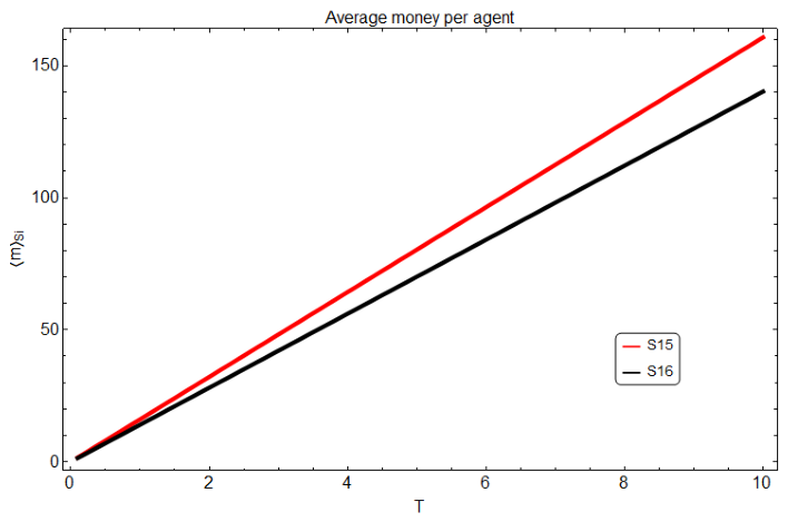
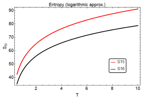
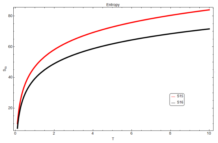
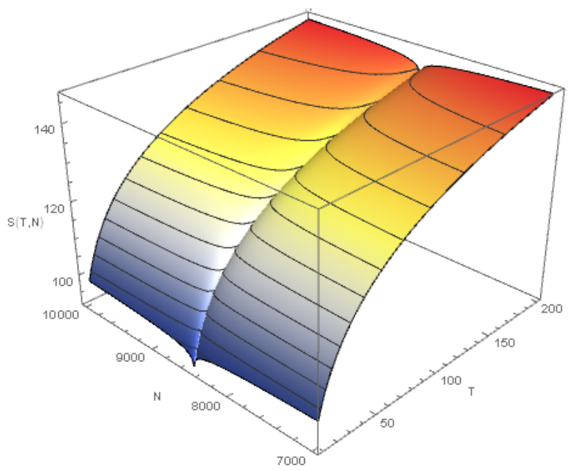
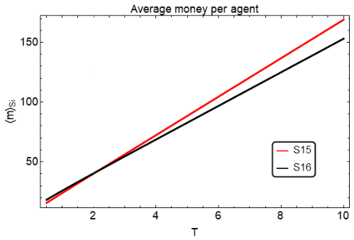
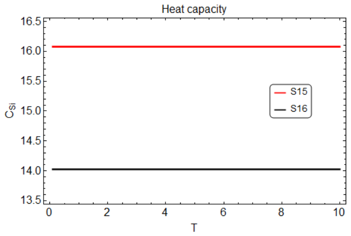
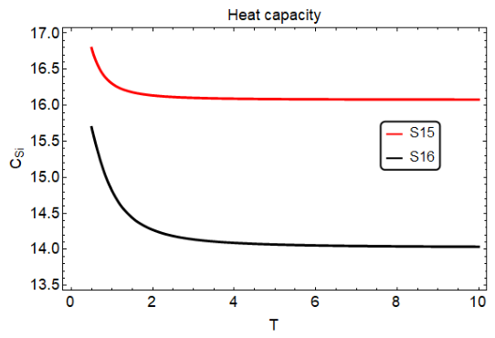
The expressions (20)–(24) follow from the multiplicative power-law ansatz (16), in which the macroeconomic variables enter as fixed external factors. Figure 1 compares the entropies $S_{S_i}$ of sectors $S_{15}$ and $S_{16}$ obtained from (22), Figure 2 the corresponding average money per agent $\langle m_{S_i}\rangle$ from (23), and Figure 3 the heat capacities $C_{S_i}$ from (24). In Section 5, we relax this form and adopt an additive logarithmic coupling for the macroeconomic block; the structure of the partition function changes accordingly, as made explicit there.

A first approximation to the inter-sectoral dynamics treats sectors $S_{15}$ and $S_{16}$ as a closed economic subsystem with respect to the remaining CSDB. Over the analysed time window, net monetary flows across the boundary of this two-sector system are negligible compared to internal transfers. Consequently, the total economic energy(money) within the subsystem is approximately conserved, leading to the internal balance condition $\Delta Q_{S_{15}}+\Delta Q_{S_{16}}=0$. Each sector is characterised by its heat content $Q_{S_i}$ and economic temperature $T_{S_i}$. CSDB data indicate $T_{S_{15}}>T_{S_{16}}$, so a heat-like transfer occurs from $S_{15}$ to $S_{16}$. According to the second law,

$$\Delta Q_{S_i}={\int }_{S_{0,S_i}}^{S_{f,S_i}}{T}_{S_i}\left(S_{S_i}\right)d{S}_{S_i}.$$

(25)

From Equations (24) and (25):

$$\Delta Q_{S_i}={\displaystyle \frac{k_{S_i}{\pi }_{\mathrm{IPP}}^{x_{S_i}}{\pi }_{\mathrm{IPC}}^{y_{S_i}}{\mathit{\lambda }}_{\mathrm{TRM}}^{z_{S_i}}}{{\left[\Gamma \left(1+\frac{1}{v_{S_i}}\right)\right]}^{v_{S_i}}}}\left({\displaystyle \frac{e^{(v_{S_i}-1)}}{v_{S_i}}}\right)\Delta S_{S_i},$$

(26)

where $\Delta S_{S_i}=S_{f,S_i}-S_{0,S_i}$. The condition $\Delta Q_{S_{15}}=-\Delta Q_{S_{16}}$ reflects internal monetary redistribution with negligible net exchange with other sectors, ensuring conservation of total money within the two-sector subsystem. Because $T_{S_{15}}>T_{S_{16}}$, sector $S_{15}$ releases heat ($\Delta S_{S_{15}}<0$, $\Delta Q_{S_{15}}<0$) while sector $S_{16}$ absorbs it ($\Delta S_{S_{16}}>0$, $\Delta Q_{S_{16}}>0$). The magnitude $|\Delta Q_{S_{15}}| = |\Delta Q_{S_{16}}|$ satisfies the conservation condition. 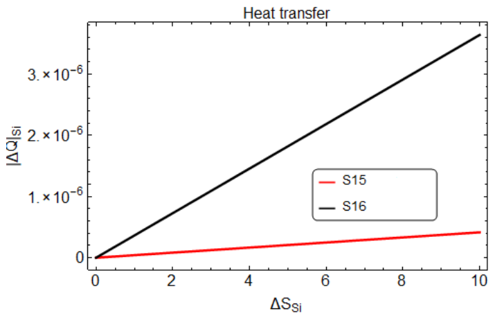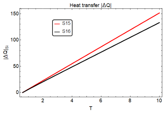Figure 4 plots $|\Delta Q_{S_i}|$ as a function of $|\Delta S_{S_i}|$; the arrows indicate the direction of the inter-sectoral heat flow $S_{15}\to S_{16}$.

5. Econophysics Approach to Sectoral Dynamics

Consider a more realistic approximation. We emphasise that the money function is now modified with respect to the multiplicative power-law ansatz of (16): the macroeconomic dependence is moved from a multiplicative factor into an additive logarithmic term. This change is deliberate. Whereas (16) is the minimal tractable form used in Section 4 to obtain the closed expressions (20)–(24), the logarithmic coupling adopted here is motivated by the result of Quevedo et al. [9] that a term $m\propto c_1\ln {\mathit{\lambda }}_1$ naturally generates Pareto-type distributions, characteristic of real economic systems. Given that the CSDB comprises 17 complementary economic activities, 5 of which account for the largest share of output, we therefore describe the money function as [9]

$$m_{S_i}(\overline{\mathit{\lambda }},\overline{\Lambda })=k_{S_i}\left[{\mathit{\lambda }}_{S_i}^{v_{S_i}}+\ln \left|{\pi }_{\mathrm{IPP}}^{x_{S_i}}{\pi }_{\mathrm{IPC}}^{y_{S_i}}{\mathit{\lambda }}_{\mathrm{TRM}}^{z_{S_i}}\right|\right].$$

(27)

The combined ansätz is not unique; it represents the simplest nontrivial extension that preserves analytical tractability while capturing both heavy-tailed scaling behaviour and the dominant macroeconomic dependences.

The partition function then becomes

$$\begin{array}{cc}\hfill Z\left(T,\overline{\mathit{\lambda }},\overline{\Lambda }\right)& ={\int }_{\overline{\mathit{\lambda }}}{\int }_{\overline{\Lambda }}\exp \left[-{\displaystyle \frac{m_{S_i}(\overline{\mathit{\lambda }},\overline{\Lambda })}{T}}\right]d\overline{\mathit{\lambda }}d\overline{\Lambda }\hfill \\ \hfill & ={\int }_0^{\infty }\exp \left[-{\displaystyle \frac{k_{S_i}{\mathit{\lambda }}_{S_i}^{v_{S_i}}}{T}}\right]d{\mathit{\lambda }}_{S_i}{\int }_{X_0}^X{\pi }_{\mathrm{IPP}}^{-A_{S_i}}d{\pi }_{\mathrm{IPP}}\hfill \\ \hfill & \times {\int }_{Y_0}^Y{\pi }_{\mathrm{IPC}}^{-B_{S_i}}d{\pi }_{\mathrm{IPC}}{\int }_{Z_0}^1{\mathit{\lambda }}_{\mathrm{TRM}}^{-C_{S_i}}d{\mathit{\lambda }}_{\mathrm{TRM}}\hfill \end{array}$$

(28)

$$=-{\displaystyle \frac{T^3\Delta X\Delta Y\Delta Z}{D_{S_i}}}{\left({\displaystyle \frac{k_{S_i}}{T}}\right)}^{-1/v_{S_i}}\Gamma \left(1+\frac{1}{v_{S_i}}\right),$$

(29)

which is positive provided $D_{S_i}>0$. The structural difference with respect to (20) is a direct consequence of the change of ansatz: under the additive logarithmic coupling of (27), the macroeconomic dependence factorises out of the Gaussian-type integral over ${\mathit{\lambda }}_{S_i}$ and is integrated explicitly over its empirical range, producing the prefactor $\Delta X\Delta Y\Delta Z/D_{S_i}$ in place of the ${\left(\frac{k_{S_i}}{T}{\pi }_{\mathrm{IPP}}^x{\pi }_{\mathrm{IPC}}^y{\mathit{\lambda }}_{\mathrm{TRM}}^z\right)}^{-1/v_{S_i}}$ block of (20). The two expressions are not in contradiction; they correspond to two distinct modelling choices for the macroeconomic sector, the multiplicative form (Section 4) and the logarithmic form (Section 5). The auxiliary variables appearing in (29) are

$$A_{S_i}={\displaystyle \frac{k_{S_i}{x}_{S_i}}{T}},B_{S_i}={\displaystyle \frac{k_{S_i}{y}_{S_i}}{T}},C_{S_i}={\displaystyle \frac{k_{S_i}{z}_{S_i}}{T}},$$

(30)

$$\Delta X=X^{1-A_{S_i}}-X_0^{1-A_{S_i}},\Delta Y=Y^{1-B_{S_i}}-Y_0^{1-B_{S_i}},$$

(31)

$$\Delta Z=1-Z_0^{1-C_{S_i}},{\Gamma }_{v_{S_i}}=\Gamma \left(1+\frac{1}{v_{S_i}}\right),$$

(32)

$$D_{S_i}=(T-k_{S_i}{x}_{S_i})(T-k_{S_i}{y}_{S_i})(T-k_{S_i}{z}_{S_i}).$$

(33)

The integration bounds X, $X_0$, Y, $Y_0$, $Z_0$ are the upper and lower limits of the normalised price indices and exchange rate over the empirical period 2018–2023. Specifically, $X_0$ and $Y_0$ are the baseline (2018) values of ${\pi }_{\mathrm{IPP}}$ and ${\pi }_{\mathrm{IPC}}$ respectively; X and Y are their maximum observed values; $Z_0$ is the minimum observed value of ${\mathit{\lambda }}_{\mathrm{TRM}}$ (equal to unity by construction in 2018); and the upper bound of ${\mathit{\lambda }}_{\mathrm{TRM}}$ is normalised to 1. The empirical ranges are read from Appendix C.

• Domain of validity.

The macroeconomic integrals in (29) converge only above a sector-dependent threshold. Writing $D_{S_i}=(T-k_{S_i}{x}_{S_i})(T-k_{S_i}{y}_{S_i})(T-k_{S_i}{z}_{S_i})$, each factor $(T-k_{S_i}e)$ with $e>0$ changes sign at $T=k_{S_i}e$, whereas factors with $e<0$ remain positive for all $T>0$. With the signed exponents of Equation (19), the only positive root for both sectors is $T=k_{S_i}{x}_{S_i}$; the macroeconomic exponents $y_{S_i},z_{S_i}<0$ introduce no pole at positive temperature. The thermodynamic description is therefore well defined for

$$T>T_{\min }\equiv k_{S_i}\max \left(\left|x_{S_i}\right|,\left|y_{S_i}\right|,\left|z_{S_i}\right|\right),$$

(34)

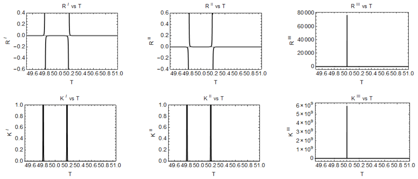
which, with $k_{S_i}\approx 1$ and the values of Table A4, gives $T_{\min }^{S_{15}}=3.353$ and $T_{\min }^{S_{16}}=6.757$. The single pole at $T=k_{S_i}{x}_{S_i}=T_{\min }$ reflects the convergence condition of the producer price-index integral and should not be interpreted as a physical phase transition; the thermodynamic quantities are reported only for $T>T_{\min }$. Figure 5, Figure 6, Figure 7 and Figure 8 are plotted accordingly.

The free money function from (2):

$${\langle m\rangle }_{S_i}=T^2{\displaystyle \frac{\partial }{\partial T}}\ln \left|-{\displaystyle \frac{T^3\Delta X\Delta Y\Delta Z}{D_{S_i}}}{\left({\displaystyle \frac{k_{S_i}}{T}}\right)}^{-1/v_{S_i}}\Gamma \left(1+\frac{1}{v_{S_i}}\right)\right|.$$

(35)

The heat capacity from (5):

$$C_{S_i}=T{\displaystyle \frac{{\partial }^2}{\partial T^2}}\ln \left|-{\displaystyle \frac{T^3\Delta X\Delta Y\Delta Z}{D_{S_i}}}{\left({\displaystyle \frac{k_{S_i}}{T}}\right)}^{-1/v_{S_i}}\Gamma \left(1+\frac{1}{v_{S_i}}\right)\right|.$$

(36)

The heat-like transfer $\Delta Q$ between $S_{15}$ and $S_{16}$ follows from (6):

$$\begin{array}{cc}\hfill \Delta Q_{S_i}& ={\int }_{T_{0,S_i}}^{T_{f,S_i}}{C}_{S_i}d{T}_{S_i}\hfill \\ \hfill & ={\int }_{T_{0,S_i}}^{T_{f,S_i}}T{\displaystyle \frac{{\partial }^2}{\partial T^2}}\ln \left|-{\displaystyle \frac{T^3\Delta X\Delta Y\Delta Z}{D_{S_i}}}{\left({\displaystyle \frac{k_{S_i}}{T}}\right)}^{-1/v_{S_i}}\Gamma \left(1+\frac{1}{v_{S_i}}\right)\right|d{T}_{S_i},\hfill \end{array}$$

(37)

where we impose $\Delta Q_{S_{15}}=-\Delta Q_{S_{16}}$ and $S_{\mathrm{Total}}=S_{S_{15}}+S_{S_{16}}$, reflecting a closed subsystem with internal monetary redistribution. The sector with $T_{S_{15}}>T_{S_{16}}$ releases heat ($\Delta Q_{S_{15}}<0$, integrated over a decreasing temperature range $T_f<T_0$), while $S_{16}$ absorbs an equal amount ($\Delta Q_{S_{16}}>0$, $T_f>T_0$).

6. GTD Approximation to the CSDB

Let the money function (27) be extended to include the number of firms $N_{S_i,f}$ in sector $S_i$:

$$m_{S_i}(\overline{\mathit{\lambda }},\overline{\Lambda })=k_{S_i}\left[{\mathit{\lambda }}_{S_i}^{v_{S_i}}+\ln \left|{\pi }_{\mathrm{IPP}}^{x_{S_i}}{\pi }_{\mathrm{IPC}}^{y_{S_i}}{\mathit{\lambda }}_{\mathrm{TRM}}^{z_{S_i}}\right|+\ln {\displaystyle \frac{N_{S_i,f}}{N_{S_i,0}}}\right],$$

(38)

where $N_{S_i,0}$ is the number of firms in sector $S_i$ at $t_0=2018$ and $N_{S_i,f}$ is the number at time t.

Integrating over all microeconomic and macroeconomic parameters, with $N_{S_i,f}$ entering as the upper limit of the integration over the firm-count variable, gives

$$Z(T,N_{S_i,f})={\displaystyle \frac{T^4\Delta N\Delta X\Delta Y\Delta Z}{D_{S_i}}}{\left({\displaystyle \frac{k_{S_i}}{T}}\right)}^{-1/v_{S_i}}\Gamma \left(1+\frac{1}{v_{S_i}}\right),$$

(39)

where the auxiliary variables (30)–(32) are supplemented by

$$A_{S_i}^{\left(N\right)}={\displaystyle \frac{k_{S_i}}{T}},\Delta N=N_{S_i,f}^{1-A_{S_i}^{\left(N\right)}}-N_{S_i,0}^{1-A_{S_i}^{\left(N\right)}},$$

(40)

$$D_{S_i}=(T-k_{S_i})(T-k_{S_i}{x}_{S_i})(T-k_{S_i}{y}_{S_i})(T-k_{S_i}{z}_{S_i}),$$

(41)

and Equation (39) is positive for $T>T_{\min }^{\left(GTD\right)}\equiv k_{S_i}·\max (1,x_{S_i},y_{S_i},z_{S_i})$.

Crucially, $N_{S_i,f}$ now enters explicitly through $\Delta N$ in Equation (40), so the partition function $Z(T,N_{S_i,f})$ and hence the entropy $S_{S_i}(T,N_{S_i,f})$ are genuine functions of two independent variables. This is essential for the well-posedness of the GTD construction.

The entropy is

$$\begin{array}{cc}\hfill S_{S_i}(T,N_{S_i})& =\ln \left|{\displaystyle \frac{T^4\Delta N\Delta X\Delta Y\Delta Z}{D_{S_i}}}{\left({\displaystyle \frac{k_{S_i}}{T}}\right)}^{-1/v_{S_i}}\Gamma \left(1+\frac{1}{v_{S_i}}\right)\right|\hfill \\ \hfill & +T{\displaystyle \frac{\partial }{\partial T}}\ln \left|{\displaystyle \frac{T^4\Delta N\Delta X\Delta Y\Delta Z}{D_{S_i}}}{\left({\displaystyle \frac{k_{S_i}}{T}}\right)}^{-1/v_{S_i}}\Gamma \left(1+\frac{1}{v_{S_i}}\right)\right|.\hfill \end{array}$$

(42)

An explicit analytic expansion of (42) is too cumbersome for the main text. Within the GTD framework, we take $\Phi =S(T,N_{S_i})$ with coordinates $E^a=\{T,N_{S_i}\}=\{E^1,E^2\}$ on the equilibrium manifold $\mathcal{E}$.

Second-Order Taylor Expansion and Non-Degenerate Hessian

A second-order Taylor series expansion of Equation (42) in two variables around the reference point $(T_0,N_{S_i,0})$ yields:

$$\begin{array}{cc}\hfill S_{S_i}(T,N_{S_i})& \approx S_0+{\alpha }_T(T-T_0)+{\alpha }_N(N_{S_i}-N_{S_i,0})\hfill \\ \hfill & +\frac{1}{2}{\alpha }_{TT}{(T-T_0)}^2+{\alpha }_{TN}(T-T_0)(N_{S_i}-N_{S_i,0})\hfill \\ \hfill & +\frac{1}{2}{\alpha }_{NN}{(N_{S_i}-N_{S_i,0})}^2,\hfill \end{array}$$

(43)

where $S_0=S_{S_i}(T_0,N_{S_i,0})$ and

$${\alpha }_T={\left.{\displaystyle \frac{\partial S}{\partial T}}\right|}_0,{\alpha }_N={\left.{\displaystyle \frac{\partial S}{\partial N_{S_i}}}\right|}_0,$$

(44)

$${\alpha }_{TT}={\left.{\displaystyle \frac{{\partial }^{2}S}{\partial T^2}}\right|}_0,{\alpha }_{TN}={\left.{\displaystyle \frac{{\partial }^{2}S}{\partial T\partial N_{S_i}}}\right|}_0,{\alpha }_{NN}={\left.{\displaystyle \frac{{\partial }^{2}S}{\partial N_{S_i}^2}}\right|}_0.$$

(45)

Defining $L=\ln \left|Z\right(T,N_{S_i}\left)\right|$, the general expressions for the first and second partial derivatives of $S=L+T{L}_T$ are:

$$\begin{array}{cc}\hfill {\alpha }_T& =2L_T^{\left(0\right)}+T_0{L}_{TT}^{\left(0\right)},\hfill \end{array}$$

(46)

$$\begin{array}{cc}\hfill {\alpha }_N& =L_N^{\left(0\right)}+T_0{L}_{TN}^{\left(0\right)},\hfill \end{array}$$

(47)

$$\begin{array}{cc}\hfill {\alpha }_{TT}& =3L_{TT}^{\left(0\right)}+T_0{L}_{TTT}^{\left(0\right)},\hfill \end{array}$$

(48)

$$\begin{array}{cc}\hfill {\alpha }_{TN}& =2L_{TN}^{\left(0\right)}+T_0{L}_{TTN}^{\left(0\right)},\hfill \end{array}$$

(49)

$$\begin{array}{cc}\hfill {\alpha }_{NN}& =L_{NN}^{\left(0\right)}+T_0{L}_{TNN}^{\left(0\right)},\hfill \end{array}$$

(50)

where superscript $\left(0\right)$ denotes evaluation at $(T_0,N_{S_i,0})$ and subscripts denote partial differentiation. The N-derivatives of L arise from the explicit $N_{S_i,f}$ dependence in $\Delta N$ (Equation (40)):

$$L_N={\displaystyle \frac{\partial \ln |\Delta N|}{\partial N_{S_i}}}={\displaystyle \frac{(1-k_{S_i}/T)N_{S_i}^{-k_{S_i}/T}}{\Delta N}},$$

(51)

$$L_{NN}={\displaystyle \frac{{\partial }^2\ln |\Delta N|}{\partial N_{S_i}^2}}={\displaystyle \frac{-(k_{S_i}/T)(1-k_{S_i}/T)N_{S_i}^{-k_{S_i}/T-1}\Delta N-{(1-k_{S_i}/T)}^2{N}_{S_i}^{-2k_{S_i}/T}}{\Delta N^2}}.$$

(52)

These expressions are non-zero in general, ensuring ${\alpha }_N\ne 0$ and ${\alpha }_{NN}\ne 0$. The mixed coefficient ${\alpha }_{TN}$, by contrast, is found to be numerically negligible at the reference point (Appendix E), indicating a near-complete decoupling between temperature fluctuations and firm-count variations there.

The Hessian matrix of S at the reference point is

$${\mathcal{H}}^{\left(0\right)}=\left(\begin{array}{cc}{\alpha }_{TT}& {\alpha }_{TN}\\ {\alpha }_{TN}& {\alpha }_{NN}\end{array}\right),$$

(53)

with determinant

$$\det {\mathcal{H}}^{\left(0\right)}={\alpha }_{TT}{\alpha }_{NN}-{\alpha }_{TN}^2.$$

(54)

The GTD metric $g^{\mathrm{I}}$ (Equation (9)) with $\Phi =S$, ${\beta }_S=1$, and ${{\delta }^c}_a=\mathrm{diag}(1,1)$ then reads

$$g_{ab}^{\mathrm{I}}=S(T,N_{S_i})·{\mathcal{H}}_{ab}^{\left(0\right)},$$

(55)

i.e., $g^{\mathrm{I}}=S·{\mathcal{H}}^{\left(0\right)}$ with components

$$\begin{array}{cc}\hfill g_{11}^{\mathrm{I}}& =S{\alpha }_{TT},g_{12}^{\mathrm{I}}=g_{21}^{\mathrm{I}}=S{\alpha }_{TN},g_{22}^{\mathrm{I}}=S{\alpha }_{NN}.\hfill \end{array}$$

(56)

The metric is non-degenerate provided $\det g^{\mathrm{I}}=S^2\det {\mathcal{H}}^{\left(0\right)}\ne 0$, which requires $S\ne 0$ and $\det {\mathcal{H}}^{\left(0\right)}\ne 0$. Numerical evaluation at $(T_0,N_{S_i,0})=(50,8500)$ for sector $S_{15}$ and $(50,9500)$ for sector $S_{16}$ (Appendix E), performed with arbitrary-precision arithmetic, gives $\det {\mathcal{H}}^{\left(0\right)}>0$ in both cases, validating the computation of curvature invariants from Equation (55).

For a 2D metric of the form $g_{ab}=f(T,N_{S_i})·c_{ab}$ with constant $c_{ab}={\mathcal{H}}_{ab}^{\left(0\right)}$, the Ricci scalar is

$$R^{\mathrm{I}}=-{\displaystyle \frac{1}{f}}{\nabla }^2\left(\ln f\right),$$

(57)

where $f=S(T,N_{S_i})$ and ${\nabla }^2$ is the Laplacian in the metric induced by $c_{ab}$. With S approximated by the second-order expansion (43), this yields a non-trivial $R^{\mathrm{I}}$ that diverges only when $S\to 0$, i.e., at the zeros of the entropy function.

The regularity of the equilibrium manifold is governed by the exact entropy $S(T,N_{S_{i,0}})$, which acts as the conformal factor of all three Legendre metrics (Appendix F). Direct evaluation of the exact expression (42) with the numerically converged derivatives of Appendix E shows that $S(T,N_{S_{i,0}})$ is strictly positive and monotonically increasing throughout the empirically relevant range $T\in \left[1,200\right]$, with no zero, maximum or inflection in this interval for either sector. Since the curvature scalars diverge only at the zeros of the conformal factor, the absence of any zero of the exact entropy in the data domain guarantees that $R^I$ and $K^I$ are finite and regular over the entire range. Crucially, this conclusion is a property of the exact entropy and is therefore independent of the expansion point: it does not rely on the location of the zeros of the second-order Taylor surface, which serves here only as a local computational device for the Hessian (the “Second-Order Taylor Expansion and Non-Degenerate Hessian” subsection). The equilibrium manifold thus exhibits no geometric phase transition in the period under study.

The curvature scalars of Figure 9, Figure 10, Figure 11 and Figure 12 confirm the regularity established analytically. In the temperature sections (Figure 9 and Figure 11, $N_{S_i}=N_{S_i,0}$ fixed) the Ricci and Kretschmann scalars of all three Legendre metrics remain finite and of small magnitude across $T\in [1,100]$ for both sectors: $R^{\mathrm{I}}$ and $R^{\mathrm{II}}$ vary monotonically while $R^{\mathrm{III}}$ (and the corresponding K) traces a shallow parabola about the expansion point $T_0=50$, with no divergence—consistent with the strict positivity of the exact entropy over the empirical range (Appendix G). The firm-count sections (Figure 10 and Figure 12, $T=T_0$ fixed) appear to diverge near $N_{S_i}\simeq N_{S_i,0}$, but this feature is not physical: because ${\alpha }_{NN}<0$, the second-order entropy is concave in $N_{S_i}$ and remains positive only within $|N_{S_i}-N_{S_i,0}| \lesssim 0.014N_{S_i,0}$, so the apparent poles are artefacts of extrapolating the quadratic truncation far from the expansion point (Appendix F) and are reported only for completeness. Taken together, the panels show that the equilibrium manifold is geometrically regular over the economically meaningful domain and that this conclusion is independent of the metric ($g^{\mathrm{I}}$, $g^{\mathrm{II}}$ or $g^{\mathrm{III}}$), the three differing only in the sign and scale of the scalars, not in their singular locus.

7. Discussion and Conclusions

This work proposes an econophysics approach to the sectoral dynamics of Bogotá’s Sports Satellite Account (CSDB), grounded in statistical thermodynamics and GTD. This conceptual framework enables the interpretation of the economy as a complex system in which money plays a role analogous to energy, and thermodynamic quantities acquire well-defined economic meanings. In particular, sectors $S_{15}$ (gambling and betting) and $S_{16}$ (recreational and sports activities) provide an illustrative contrast.

In the present framework, the introduction of economic heat and economic work is not merely formal. Following interpretations proposed in economic thermodynamics [33,34,35], economic heat is associated with monetary transfers that modify the internal state of the system without directly generating productive output—such as redistribution mechanisms, subsidies, or exogenous injections.

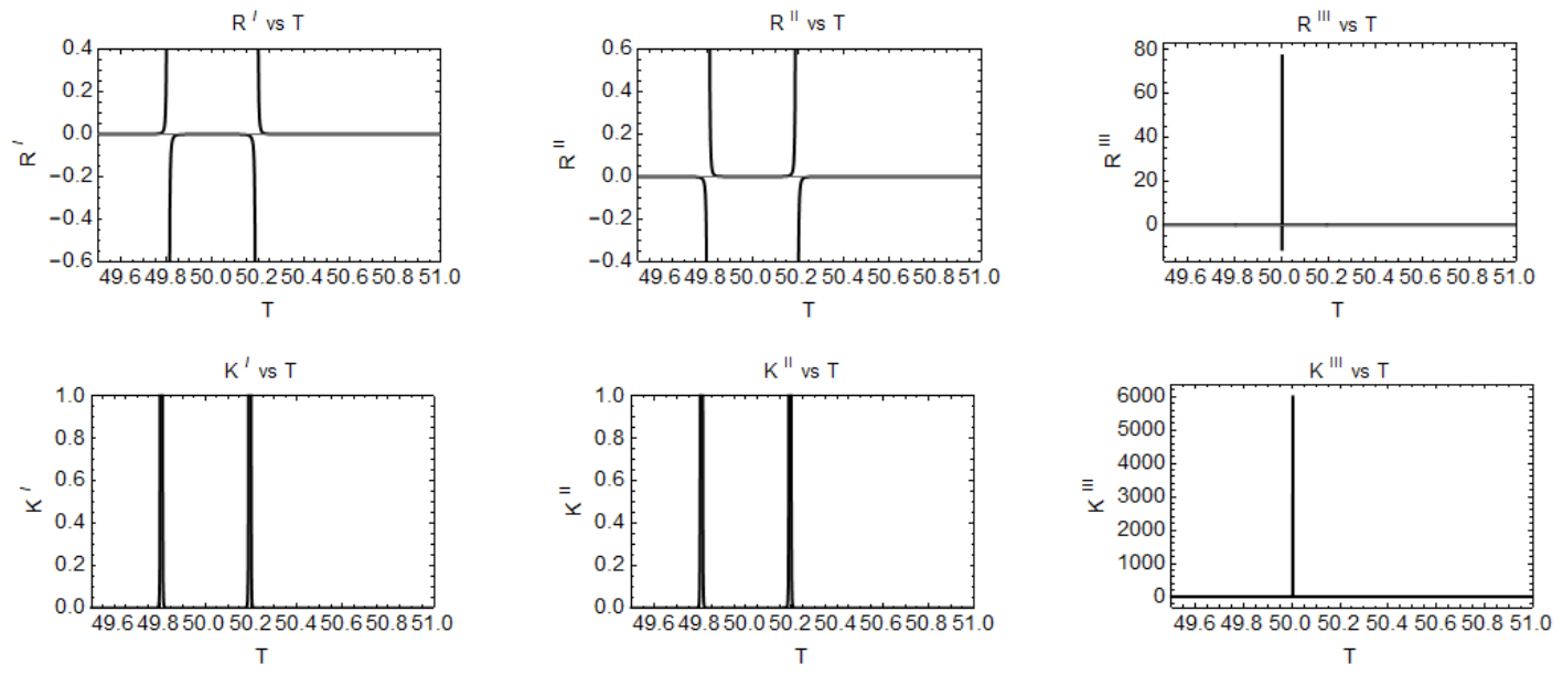
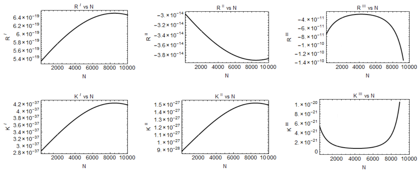
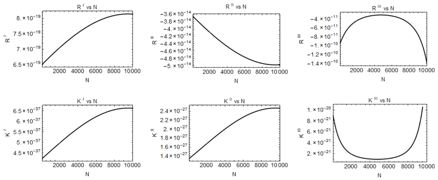
The geometrothermodynamic analysis of the equilibrium manifold $\mathcal{E}$ yields the central structural result of this study. Computing the Ricci and Kretschmann scalars for the three Legendre-invariant metrics $g^{\mathrm{I}}$, $g^{\mathrm{II}}$ and $g^{\mathrm{III}}$ with a numerically converged Hessian (Appendix E), we find that the curvature invariants are finite and regular throughout the empirically relevant domain: the exact entropy $S(T,N_{S_i,0})$ is strictly positive throughout the data domain and has no zero there, so the conformal factor controlling the curvature never vanishes and no geometric phase transition occurs within the period studied (Figure 9 and Figure 11). Because this is a property of the exact entropy rather than of the local Taylor surface, the diagnostic is independent of the expansion point $T_0$, as verified explicitly by the sensitivity analysis of Appendix G.

We state this finding explicitly, as it is the central empirical result of the present analysis: the equilibrium geometry is regular over the entire sample, and the 2020 contraction is not reflected as a curvature singularity. The smoothness of the equilibrium manifold indicates that the sectoral system absorbed the macroeconomic disruptions of 2018–2023 without an abrupt change in its underlying geometric structure. The 2020 minimum, though clearly visible in the raw series (Appendix B), thus remains an empirical feature of the time series and does not constitute a geometric phase transition; we therefore refrain from interpreting it as one. Crucially, this conclusion is independent of the metric chosen: the three Legendre metrics share the same conformal factor S and hence the same (out-of-range) singular locus, differing only in the sign and magnitude of the scalars (Appendix F).

These results should be read as qualitative structural indicators rather than predictive signals, and are subject to the intrinsic limitation of the present dataset: the annual resolution of the CSDB ($n=6$ observations per sector) restricts the statistical power of individual coefficient inference and the temperature range over which the second-order expansion is locally valid. In particular, the microeconomic exponent $v_{S_i}=\left|b_1\right|$ is not resolved in sign by the data at this resolution; its positivity is fixed instead by the convergence requirement of the partition function (Appendix D.4). This indeterminacy does not, however, propagate to the geometric diagnostic: the strict positivity of the conformal factor S and the finiteness of the curvature scalars $R^{\mathrm{I}}$ and $K^{\mathrm{I}}$ remain stable under a tenfold variation of $v_{S_i}$, as does the non-degeneracy of the metric (Appendix I). Together with the robustness already established against the expansion point $T_0$ (Appendix G) and the regularisation parameter $\epsilon$ (Appendix H), this confirms that the central structural finding does not rest on any statistically undetermined quantity. Accordingly, the approach is best understood as a complementary, geometry-based framework for assessing economic equilibrium stability, not a replacement for standard economic models.

For future research, we propose extending this analysis to all 17 sectors of the CSDB; incorporating longer and higher-frequency time series to validate model robustness and to probe whether genuine curvature singularities emerge at finer temporal resolution; benchmarking against conventional macroeconomic indicators; and enriching the partition function with microeconomic data on agent counts, firm-size distributions, and consumption patterns.