


Abstract
This paper studies transfer learning for ridge-regularized robust linear regression in the moderate–dimensional regime, where the number of predictors is of the same order as the sample size and the regression coefficients are not assumed to be sparse. We propose Trans-RR, which combines a robust ridge estimator from a source study with a robust ridge correction based on the target study. Under mild assumptions, we characterize the asymptotic estimation error of the proposed estimator and show that leveraging source data can substantially improve estimation accuracy relative to the traditional single-study ridge-regularized robust estimator. To guard against negative transfer when the source study is not sufficiently informative, we further propose an adaptive aggregation of Trans-RR with the single-task estimator that selects the mixing weight by cross-validation. Simulation studies and a real-data analysis support the theory and illustrate the transition between positive and negative transfer as the discrepancy between the source and target studies varies.
1. Introduction
Modern statistical analyses often involve several related datasets collected from different studies, populations, or experiments. A basic question is how to use these datasets together to improve prediction and estimation for a study of interest. Transfer learning addresses this question by borrowing useful information from related tasks. It is now standard in machine learning and has been successful in applications such as natural language processing, remote sensing, and computer vision [1,2,3]. In statistics, it has also become an important tool for improving performance in multi-study problems.
In many contemporary applications, regression problems arise in a moderate–dimensional regime, where the number of predictors is of the same order as the sample size and sparsity is often not a reasonable structural assumption. At the same time, heavy-tailed errors or outlying observations may substantially affect estimation accuracy. This setting arises naturally in multisite metabolomics studies, where many metabolites are measured simultaneously, between-cohort heterogeneity is often present, and outliers or other data contamination can be an important practical concern [4]. These features make transfer learning particularly challenging: related source studies may contain useful information, but effective borrowing requires methods that are robust to contamination and suitable for moderate–dimensional, non-sparse settings.
Existing theoretical work on transfer learning covers several important settings. For linear regression, ref. [5] studied data-enriched regression in a fixed-dimensional setting, and ref. [6] analyzed linear models with a shared low-dimensional representation across tasks. In the high-dimensional sparse regime, ref. [7] considered transfer learning with proxy data, while ref. [8] established prediction and estimation guarantees for sparse linear regression. For high-dimensional generalized linear models, refs. [9,10] developed transfer learning methods with theoretical guarantees. Transfer learning has also been studied for nonparametric classification [11], nonparametric regression [12], and settings with unreliable source data [13]. However, these works do not apply to the moderate–dimensional robust setting considered here.
Robust regression has, in contrast, been extensively studied in the single-study setting. For classical M-estimation, a substantial body of work has established asymptotic results when while , including [14,15,16,17,18,19]. When , robust regression has a qualitatively different asymptotic behavior [20]. When , ref. [21] proposed a ridge-regularized robust estimator to address the nonexistence of the ordinary robust estimator. However, these results do not directly extend to the transfer learning framework when related source data are available.
Motivated by these gaps, we study transfer learning under a moderate–dimensional robust linear model with one target study and one related source study. We allow the predictor dimension to be of the same order as the target and source sample sizes, do not impose sparsity assumptions on the regression coefficients, and permit heavy-tailed errors. Within this framework, our goal is to leverage information from the source study to improve the estimation performance of traditional single-task approaches.
Our main contribution is to develop and analyze a transfer learning method for moderate–dimensional ridge-regularized robust linear regression. First, we propose Trans-RR, a transfer learning procedure for ridge-regularized robust linear regression. It combines a robust ridge fit on the source study with a robust ridge correction on the target study and is designed for non-sparse coefficients. Second, we derive an asymptotic characterization of the risk of the resulting estimator under mild assumptions on the design and error distributions. The theory shows how auxiliary source data can improve estimation accuracy relative to the single-study ridge-regularized robust estimator, while also clarifying the possibility of negative transfer. Third, we propose an adaptive aggregation of Trans-RR with the single-task estimator that selects the mixing weight by cross-validation, providing a data-driven safeguard against negative transfer. Fourth, we conduct simulation studies and a real-data analysis to examine the practical performance of the proposed methods, including their sensitivity to tuning choices and to the identity–covariance assumption underlying the theory.
The rest of the paper is organized as follows. Section 2 introduces the model setup and the proposed algorithm. Section 3 presents the technical assumptions, the theoretical results, and the adaptive aggregation against negative transfer. Section 4 presents simulation studies to evaluate the performance of the proposed methods. Section 5 applies the proposed methods to a real-data example. The proofs of the main theoretical result as well as the lemmas are included in Appendix D and Appendix E.
Notation. Denote by the identity matrix. Let and be the vectors of zeros and ones, respectively. For a vector , the norms are , whereas . For an matrix , denote by and the maximum and minimum eigenvalues of , respectively. The norm of is defined as .
2. Methodology
2.1. Problem Setup
We consider a transfer learning problem with one target study and one related source study. In the target study, we observe n samples and , , generated from
where , are independently distributed errors and is the unknown regression parameter of interest.
In addition to the target data, we observe samples , , from the source study satisfying
where is the regression parameter for the source study and , are independently distributed errors. Throughout, both and are allowed to be heavy-tailed.
We work in the moderate–dimensional regime, where p is of the same order as both n and , with and . We also do not impose sparsity assumptions on or . Let denote the source–target discrepancy and let measure its size. Smaller values of h correspond to a more informative source study and hence a greater potential for useful transfer.
2.2. Trans-RR Algorithm
Based on this setup, we now introduce the proposed transfer learning algorithm, referred to as Trans-RR. Following the general two-stage strategy used in [7,8,9], the core of the procedure consists of two estimation steps. The first step estimates the source coefficient vector from the source data. The second step estimates the source–target discrepancy from the target data, after which the two estimates are combined. Algorithm 1 summarizes the procedure.
| Algorithm 1: Trans-RR algorithm |
|
Input: target data and source data Output: the estimated coefficient vector Step 1. Compute for some constant . Step 2. Compute for some constant . Step 3. Let Step 4. Output . |
The idea behind the construction is straightforward. Step 1 computes a ridge-regularized robust estimator from the source study. Step 2 then estimates the discrepancy relative to the source-stage fit by solving a second ridge-regularized robust regression problem on the target study. The final estimator is obtained by combining these two pieces, namely . The main difference between our procedure and those of [7,8,9] is that we use ridge/ regularization in both steps, whereas they use regularization. This choice is motivated by our diffuse-coefficient setting: the regression parameters and have many small coordinates and are not well approximated by sparse vectors. In this setting, lasso-based methods are not well-suited to the problem, whereas ridge penalization is natural. Another difference is that we use robust loss functions rather than the quadratic loss, which makes the procedure less sensitive to outliers and heavy-tailed errors.
Remark 1.
When robustness to heavy-tailed errors or outliers is needed, Huber-type loss functions are natural candidates for ρ and . Specific choices of ρ and under our theoretical framework are discussed in Section 3. The regularization parameters τ and may be selected by standard data-driven tuning methods such as cross-validation.
3. Theoretical Results
This section introduces the assumptions for the analysis and then presents the main asymptotic error results for Trans-RR.
3.1. Technical Assumptions
We study the estimation error of the estimator in Algorithm 1 under the following assumptions. We state the assumptions separately for the target study (Assumption 1) and the source study (Assumption 2), since the two stages are based on different samples. The two sets of conditions are largely parallel.
Assumption 1.
- (a)
- .
- (b)
- Suppose ρ is an even and convex function. Assume that is bounded and is Lipschitz and bounded. Moreover, we assume that and that for all .
- (c)
- Assume that there exist independent variables ’s and ’s such that . Suppose that ’s are i.i.d. with independent entries, and they have mean and . Suppose there exist and that vary with n, where and is bounded in n, such that for any convex 1-Lipschitz function G of , holds for all , where is the median of . We require the same assumption to hold for the columns of the design matrix . Additionally, we assume that the coordinates of have moments of all orders, and the k-th moment of the entries of is assumed to be uniformly bounded independently of n and p for all k.
- (d)
- Suppose that ’s are independent, with , being bounded, and growing at most like for some k. ’s may have finitely many possible distributions.
- (e)
- Suppose that ’s are independent and are also independent of ’s and ’s. They may have finitely many possible distributions, each with a density that is differentiable, symmetric, and unimodal. If is the density of one such distribution, we assume that .
- (f)
- The fraction of occurrences for each possible combination of distributions for has a limit as .
- (g)
- There exist constants and such that and .
Assumption 2.
- (a)
- .
- (b)
- and satisfy Assumption 1(b).
- (c)
- , ’s and ’s satisfy Assumption 1(c).
- (d)
- ’s satisfy Assumption 1(d).
- (e)
- ’s, ’s and ’s satisfy Assumption 1(e).
- (f)
- ’s and ’s satisfy Assumption 1(f).
- (g)
- remains bounded. Furthermore, , where .
For Assumptions 1(b) and 2(b), it is quite common in robust statistics to require to be bounded. For example, the Huber loss
is chosen to grow linearly to infinity, which reduces the influence of outliers on the resulting regression estimator. Although the Huber loss does not fully satisfy the assumptions because it is not differentiable at , these assumptions hold for a smoothed approximation such as
where . The corresponding is given by
Another example that fully satisfies the assumptions is the pseudo-Huber loss function from [22,23], defined by
The assumptions on ’s and ’s, in particular that they have mean and covariance matrix , are common in the study of M-estimators for linear models. These assumptions have been used in the low-dimensional regime studied in [14,15,24], in the moderate–dimensional regime considered in [20], and in the regime analyzed in [21,25].
The concentration assumption on ’s and ’s is weaker than the Gaussian assumptions often imposed in robust statistics. This assumption has also been studied in [21,26] and holds for a broad class of distributions. Corollary 4.10 in [27] demonstrates that our assumptions are satisfied if has independent entries bounded by for some . Additionally, Theorem 2.7 in [27] shows that the assumptions hold when has independent entries with density , , such that and for some . In particular, this condition holds when has i.i.d. entries, where . As will be seen in the proof, the functions G that arise in our analysis are either linear functions or square roots of quadratic forms. A similar discussion applies to the ’s.
The introduction of and , as also considered in [20,21], is used to induce a nonspherical geometry on the predictors. Although the assumption can be relaxed to the requirement that be uniformly bounded, it remains statistically important because it guarantees that in all the models we consider. This construction shows that many models can share the same covariance while exhibiting substantially different estimation errors for . This contrasts with the low-dimensional setting studied in [28], where is the key quantity for robust regression. A similar discussion applies to ’s and ’s.
In Assumptions 1(e) and 2(e), no moment restriction is imposed on the ’s and ’s. For instance, smooth symmetric log-concave densities satisfy all of these assumptions; see [29,30]. Furthermore, the Cauchy distribution also satisfies these conditions; see Theorem 1.6 in [31]. This makes the framework compatible with heavy-tailed errors, which are of particular interest in robust regression.
Assumptions 1(g) and 2(g) impose a non-sparse structure on and , meaning that these vectors cannot be well approximated by sparse vectors in norm. This setting is common in moderate–dimensional statistics and contrasts with the sparse regime, where only a small fraction of coefficients are substantial. Under these assumptions, the proposed Trans-RR estimator may outperform lasso-based methods.
We now turn to the target-stage result and the resulting error characterization for Trans-RR.
3.2. Asymptotic Characterization of Estimation Error
Our main theorem characterizes the asymptotic error of the Trans-RR estimator. Recall that is defined in (5), and let be fixed as n and p vary. To state the result, let denote the proximal mapping of the function , see [32]. It is given by
When is differentiable, is the unique satisfying , with . can be viewed as a shrinkage of x toward the minimizer of , with the amount of shrinkage depending on c and . The proximal mapping is a standard object in convex analysis and convex optimization (see [33] for a review of its analytic properties and an introduction to proximal gradient algorithms). As explained in [34], the system in Theorem 1 can be reformulated in terms of , where denotes the Fenchel–Legendre conjugate of f.
Under Assumptions 1 and 2, the estimation error admits the following limit.
Theorem 1.
Under Assumptions 1 and 2, conditional on the source-stage estimator , which is independent of the target sample, we have in probability, where is deterministic for the given value of . Let , where is a standard normal random variable independent of and . Then there exists a constant such that
The proof of Theorem 1 is given in Appendix E. Here and below, the dependence of and on is suppressed for notational simplicity.
Theorem 1 shows that the asymptotic error depends on the source study only through the discrepancy . To investigate when positive transfer occurs, Section 4.2 numerically computes as a function of under the smoothed Huber loss (6) in three simulation cases. The resulting curves are monotonically increasing across the displayed range. By the triangle inequality,
The right-hand side is the sum of the population gap between the source and target coefficients and the source-stage estimation error. Transfer is therefore expected to help when the source-stage estimator is accurate and close to the target coefficient, and to hurt when either the population gap or the source-stage estimation error is large. In practice, Section 3.3 develops an adaptive Trans-RR estimator to avoid negative transfer.
Unlike several recent transfer learning analyses, such as [7,8,9], our theory does not impose direct structural restrictions on , the difference between the target and source coefficients. Theorem 1 also shows that the performance of depends on the distribution of the ’s in the representation from Assumption 1(c). Thus, in the moderate–dimensional regime, the geometry of the target predictors encoded by materially affects the estimation error. This again contrasts with low-dimensional robust regression, where is the dominant quantity.
When for all i and the errors are i.i.d., Theorem 1 simplifies as follows.
Corollary 1.
Under the same assumptions as in Theorem 1, if for all i and the errors are i.i.d., then, conditional on , we have in probability, where is deterministic for the given value of . Let , where ϵ has the same distribution as the ’s and z is a standard normal random variable independent of ϵ. Then there exists a constant such that
Corollary 1 shows that, under a homogeneous target design, the general characterization in Theorem 1 reduces to a simpler scalar system. This special case is useful for interpretation and will also serve as a convenient benchmark in the simulation study.
Remark 2.
The limits on the left-hand side of (10) exist because Assumption 1(f) guarantees convergence of the proportions associated with each pair , where and denote the laws of and . For the second equation in (10), the ratio can be interpreted through the identity
which is well defined when . Equivalently, (10) can be written as
This representation shows that the expectation in (10) is well defined, and Assumption 1(f) ensures that the relevant limits exist.
3.3. Adaptive Aggregation Against Negative Transfer
We now develop an adaptive aggregation of Trans-RR with the single-task estimator to address negative transfer. Specifically, let denote the single-task ridge-regularized robust estimator on the target sample,
for some constant . Theorem 1 and the discussion above show that negative transfer may happen when the target–source discrepancy or the source-stage estimation error is too large. We therefore propose the adaptive Trans-RR estimator to avoid negative transfer, defined for by
Intuitively, recovers Trans-RR at and the single-task estimator at . Including both endpoints allows the procedure to fall back to either Trans-RR or the single-task estimator, while interior values allow partial transfer. We select the mixing weight from data by cross-validation and write for the resulting estimator.
We tune the ridge penalties before selecting . The source penalty is tuned by cross-validation on the source sample, yielding via (3). With fixed, the target penalty is tuned by cross-validation on the target sample through (4). The single-task penalty is tuned by cross-validation on the target sample. To select , we then use a K-fold partition of the target sample, drawn independently of the partitions used to tune and . Here, denotes the validation index set of fold k.
For each , let be the output of Algorithm 1 applied to the full source data and at the tuned . Let be the solution of (11) on at the tuned . We reuse , , and across all K folds rather than re-tuning per fold, which would multiply the penalty-tuning cost by K. We then choose
where is a validation loss and is a finite candidate set. A natural default is the absolute-error loss , which matches the criterion used to tune the ridge penalties. We refer to as the adaptive Trans-RR estimator, denoted Trans-RR-Ada in the following numerical experiments. Algorithm 2 summarizes the procedure.
| Algorithm 2: Adaptive Trans-RR algorithm |
|
Input: target data , source data , fold count K, candidate set , validation loss L Output: the adaptive estimator and the selected weight Step 1. Tune , , and by cross-validation on the corresponding samples. Compute from Algorithm 1 and from (11). Step 2. Draw a K-fold partition of the target indices, independent of the partitions used in Step 1. Step 3. For each , let be the output of Algorithm 1 applied to the full source data and at the tuned . Let be the solution of (11) on at the tuned . Step 4. Compute |
3.4. Applicability and Limitations
Theorem 1 and Corollary 1 are derived under Assumptions 1 and 2, which include three structural conditions: identity covariance , the moderate–dimensional regime , and a twice-differentiable robust loss. Under these assumptions, the asymptotic estimation error of Trans-RR equals the deterministic limit , in agreement with the numerical results of Section 4. When any of these assumptions fails, Theorem 1 no longer applies.
The adaptive aggregation of Section 3.3, by contrast, is constructed without invoking these structural assumptions. Its mixing weight is selected by cross-validation on the target sample and serves as a data-driven safeguard against negative transfer. Section 4.4 provides numerical support under AR(1)-correlated predictors across all three noise cases: a transition between positive and negative transfer is observed near , and Trans-RR-Ada continues to track the better of the two base estimators.
4. Simulation
In this section, we conduct numerical studies to support the theoretical results. We set the dimension of both target and source data to be . We set and , corresponding to moderate–dimensional settings with and . To generate data, we set and , where and have i.i.d. entries. We consider three different cases for the choices of ’s, ’s, ’s and ’s:
- Case I: for and for . The target errors are i.i.d. , and the source errors are i.i.d. .
- Case II: The variables and are i.i.d. Unif, while and are i.i.d. and , respectively.
- Case III: In both the target and source studies, half of the observations are generated as in Case and the other half are generated as in Case .
Case is a standard Gaussian setup for linear regression. Case features a non-Gaussian design and heavy-tailed errors. Case is a mixture of the two cases and is designed to test the effectiveness of our theoretical results under non-identical ’s and ’s.
4.1. Validity of Theoretical Results
We first evaluate the validity of the proposed scalar in Theorem 1. For each setting, we generate and once with i.i.d. Unif entries and set and . This construction yields diffuse coefficients whose Euclidean norms remain bounded as n grows. These coefficient vectors are fixed across the 1000 replications, while the target and source samples are regenerated in each replicate. In each replicate, we first compute from the source sample and then obtain by applying Algorithm 1, using the smoothed Huber loss (6) for both and with parameters and . We fix and repeat each setup 1000 times.
Figure 1 presents boxplots of the estimation error for cases – and . The red point in each boxplot marks the theoretical value , obtained by numerically solving the system in Theorem 1 under the corresponding simulation specification. We observe that the empirical distribution of is centered close to this value, and its dispersion decreases as n and p become larger. Table 1 shows the mean and standard deviation (SD) of (denoted as ) and the corresponding for each setup. As dimensionality increases, that is, as increases from 1 to 4, both the mean error and its variability increase, indicating that estimation becomes more difficult in more challenging moderate–dimensional regimes. The average estimation error also grows with heavier-tailed errors, highlighting the difficulty of estimation under such conditions. Results under case demonstrate that Theorem 1 is effective in handling non-identical ’s and ’s. Overall, the findings in Figure 1 and Table 1 align well with the theoretical predictions of Theorem 1.
Figure 1.
Boxplot of over 1000 simulations. The red point in each boxplot represents the theoretical value from Theorem 1. Panels from top to bottom are for , respectively, while panels from left to right are for cases , respectively.
Table 1.
Mean and SD (in parentheses) of (denoted as ) and the corresponding over 1000 simulations. Rows are indexed by , with when and when .
4.2. Theoretical Estimation Error Curves
We take to be our recommended smoothed Huber loss (6) with and fix . We numerically solve the associated scalar system while varying the discrepancy term that enters the second equation of Theorem 1. Figure 2 plots the resulting curves of for five values of under cases –. In all three cases, the curves are monotonically increasing over the displayed range, so a larger corresponds to a larger asymptotic estimation error in this setting.
Figure 2.
Theoretical curves of as a function of for five values of under cases –, obtained by numerically solving Corollary 1. The three panels correspond to cases , , and , respectively.
4.3. Comparison with Existing Methods
To evaluate when transfer is beneficial, we compare our method with several competing procedures across the three scenarios described above. We set , and . We generate , where has i.i.d. Unif entries. To control the transfer strength , we set
and define the source coefficient by . By varying from to , we obtain h ranging from approximately to , providing a comprehensive evaluation across different levels of source-target similarity. For each value of , the pair is fixed across the 500 replications, and only the data are regenerated.
We compare four ridge-type methods (Single-RR, Trans-RR, Trans-RR-Ada, and Pooled-RR) and two lasso baselines (Single-Lasso and Trans-Lasso):
- Single-RR: The single-task estimator in (11), fit to the target sample alone.
- Trans-RR: The two-stage estimator in (5), computed by Algorithm 1.
- Trans-RR-Ada: The adaptive aggregate in (12), computed by Algorithm 2 with , absolute-error loss , and weight grid .
- Pooled-RR: The same robust ridge fit applied to the concatenation of the source and target samples.
- Single-Lasso: The lasso on the target sample, with its regularization parameter chosen by -fold cross-validation.
- Trans-Lasso: The two-stage transfer-lasso of [8], in which a cross-validated source-stage lasso estimates and a cross-validated target-stage lasso fits the residual on the target sample.
The four ridge-type methods all use the smoothed Huber loss (6) with . Each ridge penalty is tuned by -fold cross-validation under the mean absolute error criterion, over the grid . For Trans-RR, the source penalty in (3) is tuned on the source sample, yielding as the minimizer of (3) at the tuned . With held fixed, the target penalty in (4) is then tuned on the target sample.
Performance is summarized by the relative estimation error . Figure 3 presents boxplots of these errors on a logarithmic scale, for varying values of h across cases –. We report all six estimators under Case . In Cases and , the noise is heavy-tailed, and the lasso methods are not designed for robustness. Their fits failed to converge to stable estimates, so we restrict these two cases to the ridge-type methods.
Figure 3.
Boxplots of relative estimation errors (log scale) across 500 replications for varying under cases –, with and . Case includes all six methods, while cases and include only the four ridge-type procedures. Panels from top to bottom are for cases , respectively.
Under Case , Trans-RR compares favorably with both lasso baselines, consistent with the non-sparse structure assumed throughout the paper. Among the ridge-type methods, Trans-RR outperforms Pooled-RR for small and moderate h across all three cases. Pooled-RR fits the source and target observations together as if they shared one coefficient, so its error reflects two mismatches: the gap between and , and the difference between source and target noise levels. As h decreases, the gap between Pooled-RR and Trans-RR narrows, in line with the theoretical expectation that smaller h indicates greater similarity between the two domains.
More importantly, the comparison with Single-RR reveals the transition between positive and negative transfer. When h is small, Trans-RR achieves the lowest relative error among the ridge-type methods. As h grows, its advantage shrinks and eventually reverses. In our experiments, this turnover occurs near . This is consistent with the numerical evidence in Section 3, since transfer is more favorable when the source-stage estimator is closer to the target coefficient. The same qualitative pattern appears in Cases and , where the transition near persists under heavy-tailed errors and heterogeneous designs.
Trans-RR-Ada provides a data-driven safeguard against this negative transfer. Figure 3 shows that it tracks the better of Single-RR and Trans-RR for every value of h. For small h, Trans-RR-Ada essentially coincides with Trans-RR, while for large h it coincides with Single-RR. At the transition , where Single-RR and Trans-RR are comparable, Trans-RR-Ada stays close to the better one.
4.4. Robustness to Non-Identity Covariance
The asymptotic theory in Section 3 assumes . To verify that our methods remain effective under non-identity covariance, we re-run the comparison of Section 4.3 under AR(1) covariance with , across all three noise cases , , and . All other settings, including the four ridge-type methods Single-RR, Trans-RR, Trans-RR-Ada, and Pooled-RR and the tuning protocol, match Section 4.3.
Figure 4 reports the resulting boxplots. The qualitative pattern of the i.i.d. comparison persists in all three cases. For small h, Trans-RR achieves the lowest error among the ridge-type methods. As h grows, its advantage shrinks and eventually reverses, with the transition again occurring near . Trans-RR-Ada tracks the better of Single-RR and Trans-RR across all values of h. The negative-transfer transition and the safeguard role of Trans-RR-Ada are therefore not specific to the identity–covariance assumption underlying Theorem 1. This suggests that Trans-RR may remain effective under non-identity covariance.
Figure 4.
Robustness check under AR(1) correlated predictors. Boxplots of relative estimation errors (log scale) across 500 replications for varying under cases – with , where and . Panels from top to bottom are for cases , , and , respectively. The four ridge-type procedures, Single-RR, Trans-RR, Trans-RR-Ada, and Pooled-RR are shown.
4.5. Sensitivity to Tuning Choices
The comparison in Figure 3 fixes the smoothed Huber loss with and selects each ridge penalty by -fold cross-validation under the mean absolute error criterion, on a common geometric grid of nine values from to 9. This subsection examines whether the qualitative findings of that comparison are stable under perturbations to four tuning choices: the smoothed Huber parameters , the cross-validation criterion, the robust loss family, and the ridge penalty grid. Each perturbation re-runs the full simulation with replications per setting.
4.5.1. Choice of
The default is the standard Huber tuning. The smoothing parameter closely approximates the unsmoothed Huber loss and keeps twice continuously differentiable, as required by Assumption 1(b). In the sensitivity experiment, we vary over and over , giving nine pairs, and re-run the full simulation across the three cases and seven discrepancy values h for every pair. Within each combination, varying the pair over the nine settings changes each method’s mean error by less than (median ) of its mean. The four-method ranking matches the default ranking in 171 of the 189 cells. The qualitative findings are therefore stable under this perturbation. Table 2 displays the four method means as a heatmap at in each of the three cases. Within each grid, the entries vary only slightly and the four-method ordering is the same in every cell, illustrating the two findings stated above. Appendix B reports the heatmaps at the other six values of h, where the same pattern holds.
Table 2.
Sensitivity of relative estimation error to the smoothed Huber parameters at the transition discrepancy . Each entry reports Single-RR/Trans-RR/Trans-RR-Ada/Pooled-RR mean estimation error over replications. The three blocks correspond to the three error distributions of Section 4.3.
4.5.2. Choice of Cross-Validation Criterion
The default selects each ridge penalty by -fold cross-validation under the mean absolute error criterion. We re-run the simulation with every cross-validation loss changed to mean squared error, keeping the smoothed Huber loss for estimation. Table 3 compares the mean estimation errors under the two criteria across all cases and values of h.
Table 3.
Sensitivity of relative estimation error to the cross-validation criterion. All settings are as in Figure 3, except that every cross-validation loss (used to select , , , , and ) is changed from MAE to MSE. Each entry reports the default (MAE-CV) and the MSE-CV mean estimation error, in the format “default/MSE-CV”, over replications.
Under Case , the two criteria yield nearly identical mean errors and the same four-method ranking at every h. Under Cases and , the mean errors of all four methods become substantially larger, and two qualitative findings of Section 4.3 no longer hold. First, Trans-RR has a larger mean error than Single-RR at every h in both heavy-tailed cases, so the range on which transfer helps disappears entirely. Second, Trans-RR-Ada no longer approximates min(Single-RR, Trans-RR) in most settings of the heavy-tailed cases. This may result from the heavy tails of Cauchy errors, under which MSE-based cross-validation is more sensitive to extreme residuals than MAE-based cross-validation. MAE-CV is therefore the appropriate default for heavy-tailed errors, and the conclusions of Section 4.3 are specific to this choice.
4.5.3. Choice of Robust Loss
In order to assess the sensitivity to the specific form of the robust loss, we replace the smoothed Huber loss in (6) with the pseudo-Huber loss at the same . Table 4 compares the mean estimation errors under the two losses across all cases and values of h.
Table 4.
Sensitivity of relative estimation error to the choice of robust loss. All settings are as in Figure 3, except that the smoothed Huber loss is replaced by the pseudo-Huber loss with (the smoothing parameter is no longer needed). Each entry reports the default (smoothed Huber) and the pseudo-Huber mean estimation error, in the format “default/pseudo-Huber”, over replications.
The mean errors are nearly identical to those under the smoothed Huber loss across all 21 settings. The four-method ranking matches the default in nearly every setting, and the few mismatches involve methods whose mean errors are essentially tied. The negative-transfer transition stays at the same value of h in every case, and Trans-RR-Ada continues to track min(Single-RR, Trans-RR) as closely as under the default. The qualitative findings of Section 4.3 are insensitive to this choice, consistent with Theorem 1.
4.5.4. Choice of Ridge Penalty Grid
The four ridge penalties , , , and are tuned by -fold cross-validation over a common geometric grid of nine values from to 9. We probe the sensitivity to this grid in two complementary ways: extending the grid to wider values, and forcing all four penalties to a common fixed value with no cross-validation.
We first extend the grid to thirteen values from to 27 on the same geometric scale, which contains the default grid as a strict subset. Table 5 compares the mean estimation errors under the default and the wide grid across all cases and values of h. The impact on estimation is negligible: each method’s mean error barely changes across settings, the four-method ranking is unchanged except at settings with near-tied means, the negative-transfer transition does not move, and Trans-RR-Ada continues to track min(Single-RR, Trans-RR) as closely as under the default. The default grid is therefore wide enough on both sides, and the qualitative findings of Section 4.3 do not depend on the choice of upper or lower endpoint.
Table 5.
Sensitivity of relative estimation error to the ridge-penalty cross-validation grid. The default grid contains 9 values from to 9 on a geometric scale. The wide grid extends this to 13 values from to 27 on the same geometric scale, and contains the default grid as a strict subset. All other settings are as in Figure 3, with replications per cell. Each entry reports Single-RR/Trans-RR/Trans-RR-Ada/Pooled-RR mean estimation error.
We next force all four ridge penalties to a common fixed value , removing the ridge cross-validation entirely. Trans-RR-Ada’s mixing weight is still selected by -fold cross-validation on the target sample (Algorithm 2). Table 6 reports the mean estimation errors at the four fixed values across all cases and values of h. At every fixed , the mean error of Trans-RR grows monotonically with h in all three cases, consistent with the theoretical risk curves of Figure 2. The absolute levels and the four-method ranking do vary substantially across the four values, but the qualitative dependence on h predicted by the theory is preserved at every .
Table 6.
Sensitivity of relative estimation error to the ridge penalty value when cross-validation tuning is disabled. All four ridge penalties (Single-RR’s , Trans-RR’s and , Pooled-RR’s ) are forced to a common fixed value from . Trans-RR-Ada’s mixing weight is still selected by 5-fold cross-validation on the target sample (Algorithm 2). All other settings are as in Figure 3, with replications per cell. Each entry reports Single-RR/Trans-RR/Trans-RR-Ada/Pooled-RR mean estimation error.
The Trans-RR-Ada safeguard nevertheless remains effective: its mean error stays close to min(Single-RR, Trans-RR) in every one of the 84 settings, just as under cross-validated penalties. The agreement between Trans-RR-Ada and min(Single-RR, Trans-RR) is therefore robust to a misspecified ridge penalty.
5. Real Data Analysis
We evaluate the proposed transfer procedure on the near-infrared (NIR) spectral dataset from the 2002 International Diffuse Reflectance Conference (IDRC) “Shootout” competition. The data consist of pharmaceutical tablet measurements collected by two spectrometers, with ASSAY as the response. For each instrument, the dataset contains a training sample of size 460 and an external test sample of size 155. Each spectrum is recorded at 650 wavelengths, yielding a moderate–dimensional regression problem.
Let X and denote the spectra from the two instruments. We consider two transfer directions. In Direction A, X is the target domain and is the source domain. In Direction B, the roles are reversed. In each repetition, we randomly split the training sample of the target instrument into two parts of sizes 160 and 300. The subset of size 160 is used as the target training sample. The remaining 300 tablets are matched with their measurements from the other instrument to form the source training sample. When X is the target domain, the target fit is constructed from 160 observations in X, and the source fit is constructed from the corresponding 300 observations in . The same scheme is applied symmetrically in the reverse direction. The external test sample of the target instrument is used for evaluation. We repeat this procedure 20 times to reduce Monte Carlo variability.
The preprocessing used in both transfer directions has two stages. First, we thin the spectrum by retaining every fourth wavelength of the original 650, yielding predictors. Two considerations motivate this thinning. Adjacent NIR wavelengths record highly overlapping absorption signals, so a four-fold thinning preserves nearly all the spectral information. This is standard practice in NIR chemometrics. A step of four also gives , the same setting as in our simulations.
Second, for each domain, predictors are whitened using its own training sample,
where and are estimated from that training sample, and the same transformation is applied to the associated test sample. Whitening decorrelates the highly collinear NIR predictors so that the sample second-moment matrix of approximates , which is the design assumption underlying Theorem 1. The response is centered using the mean of the corresponding training response, and the same centering constant is used for the associated test response. All preprocessing parameters are thus estimated only on training data and carried over to the test set, avoiding information leakage.
We compare six methods: Single-RR, Trans-RR, the adaptive Trans-RR estimator from Section 3.3 (denoted Trans-RR-Ada in the table), Pooled-RR, Single-Lasso, and Trans-Lasso. For the ridge-type methods, we use the smoothed Huber loss in (6) with . All tuning parameters are selected by 5-fold cross-validation with mean absolute error as the validation criterion, from the common grid
Performance is measured by the test-set RMSE,
where and are on the original ASSAY scale (predictions are uncentered before evaluation) and in both transfer directions.
Table 7 reports the average RMSE and its standard deviation over the 20 repetitions, and Figure 5 displays the corresponding distributional information. Trans-RR achieves the smallest mean RMSE in both transfer directions, with relatively small variability across the 20 splits. The adaptive variant Trans-RR-Ada matches Trans-RR within in mean RMSE in both directions, indicating that the source and target are close enough for transfer to be uniformly beneficial on this dataset. Pooled-RR ranks third behind the two transfer-ridge methods and is uniformly dominated by Trans-RR, suggesting that naive pooling fails to account for cross-instrument differences. The lasso methods are less competitive overall, especially Single-Lasso. This is consistent with the non-sparse structure of NIR spectra, where relevant information is distributed over broad wavelength regions rather than concentrated on a small subset of predictors.
Table 7.
Prediction performance on the NIR spectral dataset over 20 repeated random splits. Each entry reports the average RMSE, with the standard deviation in parentheses.
Figure 5.
Distribution of RMSE across the 20 repeated random splits for each of the six methods, in the two transfer directions. Boxes show the inter-quartile range, whiskers extend to 1.5 × IQR, and circles mark splits beyond that.
We further checked the procedure for four starting offsets of the every-fourth-wavelength thinning and for the same procedure without whitening. Across all five resulting preprocessing variants and both transfer directions, Trans-RR and Trans-RR-Ada are the top two methods by mean RMSE, and their mean RMSE values differ by at most . Mean RMSE for all six methods in each variant and direction is reported in Appendix C. The results, together with these robustness checks, therefore support the effectiveness of the proposed Trans-RR method.
6. Discussion
This paper introduces Trans-RR, a robust transfer-learning approach for moderate–dimensional linear regression. It extends transfer-learning ideas of [7,8] to a setting with non-sparse coefficients and heavy-tailed errors, without relying on sparsity assumptions or moment restrictions on the errors. The theory and the numerical results show that negative transfer can occur when the source study is not sufficiently informative for the target study. To guard against this, we also propose an adaptive aggregation of Trans-RR with the single-task estimator that selects the mixing weight by cross-validation. The theoretical results, simulation studies, and real-data analysis support the effectiveness of both procedures. A natural direction for further study is to identify the choice of loss function that minimizes the asymptotic estimation error in our framework.
Author Contributions
Conceptualization, L.L. and X.G.; Methodology, L.L., X.G. and Z.L.; Software, L.L.; Validation, L.L.; Formal analysis, L.L.; Data curation, L.L.; Writing—original draft, L.L.; Writing—review & editing, L.L., X.G. and Z.L.; Supervision, X.G. All authors have read and agreed to the published version of the manuscript.
Funding
This research was funded by the National Natural Science Foundation of China, grant number 12471267.
Data Availability Statement
Publicly available datasets were analyzed in this study. The near-infrared spectral data are from the 2002 International Diffuse Reflectance Conference (IDRC) “Shootout” competition and can be downloaded from https://www.eigenvector.com/data/tablets/index.html, accessed on 7 May 2026. The code presented in this study is available on request from the corresponding author.
Conflicts of Interest
The authors declare no conflicts of interest.
Appendix A. Notation
For ease of reference, Table A1 collects the main symbols used throughout the paper, grouped by topic. Additional proof-level notation is introduced at the beginning of Appendix D.
Table A1.
Summary of the main symbols used in the paper.
Appendix B. Additional (δ, η) Heatmaps
This appendix reports the heatmaps at the six values of h not shown in Table 2 of the main text. The pattern at every h matches the one at . Each method’s mean error varies by less than across the nine pairs, and the four-method ranking matches the default ranking in the large majority of cells. The few rank swaps that do occur happen at small h in Cases and , where Pooled-RR, Trans-RR, and Trans-RR-Ada have nearly tied mean errors.
Table A2.
Sensitivity of relative estimation error to the smoothed Huber parameters at . Each entry reports Single-RR/Trans-RR/Trans-RR-Ada/Pooled-RR mean estimation error over replications.
Table A3.
Sensitivity of relative estimation error to the smoothed Huber parameters at . Each entry reports Single-RR/Trans-RR/Trans-RR-Ada/Pooled-RR mean estimation error over replications.
Table A4.
Sensitivity of relative estimation error to the smoothed Huber parameters at . Each entry reports Single-RR/Trans-RR/Trans-RR-Ada/Pooled-RR mean estimation error over replications.
Table A5.
Sensitivity of relative estimation error to the smoothed Huber parameters at . Each entry reports Single-RR/Trans-RR/Trans-RR-Ada/Pooled-RR mean estimation error over replications.
Table A6.
Sensitivity of relative estimation error to the smoothed Huber parameters at . Each entry reports Single-RR/Trans-RR/Trans-RR-Ada/Pooled-RR mean estimation error over replications.
Table A7.
Sensitivity of relative estimation error to the smoothed Huber parameters at . Each entry reports Single-RR/Trans-RR/Trans-RR-Ada/Pooled-RR mean estimation error over replications.
Appendix C. Robustness Checks for the Real-Data Analysis
In Section 5, we report robustness checks across two preprocessing variants: the four starting offsets of the every-fourth-wavelength thinning, and the same procedure without the whitening step (predictors still mean-centered per instrument). Table A8 reports the per-offset mean RMSE and standard deviation; Table A9 compares the whitened and the unwhitened analysis. Each entry reports the mean RMSE (with standard deviation in parentheses) over the 20 repeated random splits.
Table A8.
Per-offset prediction performance on the NIR spectral dataset. The four offsets correspond to the four starting indices of the every-fourth-wavelength thinning, each yielding predictors.
Table A9.
Comparison of mean RMSE between the whitened analysis (default) and the analysis without whitening, in both transfer directions.
Appendix D. Assumptions
Notation. Let replace a power of . Denote by the identity matrix. When this does not create problems, we also use the standard notation for . Let and be the vectors of zeros and ones, respectively. For an matrix , denote by and the maximum and minimum eigenvalues of , respectively. The norm of is defined as . We call the sample covariance matrix of ’s when ’s are known to have zero mean. We say that in if . We use the notation to represent either the interval or , as in some cases we need to localize quantities within intervals defined by two values, a and b, without knowing in advance whether or . We denote by the design matrix whose i-th row is , and by the matrix obtained by removing the i-th row of . We write for and for . For two symmetric matrices A and B, means that is positive semi-definite. For the random variable W, we use the definition . For sequences of random variables , we use the notation and when and , respectively. For a vector , the norms are , whereas . For a function f from to , denote .
In this appendix, we refine the assumptions in the main text into the forms needed for the proof of Theorem 1. The proof is divided into three parts, and each part uses a slightly different set of technical conditions. In particular, the assumptions on are specified below according to the needs of the different proof subsections, whereas the source-side conditions remain as in Assumption 2.
- Assumptions under which the whole proof goes through
- M1. .
- M2. There exists constants and such that and .
- M3. Suppose is an even function. Assume that is bounded and is Lipschitz and bounded. Moreover, we assume that and that for all .
- M4. Assume that there exist independent variables ’s and ’s such that . Suppose that ’s are i.i.d. with independent entries, and they have mean and . Suppose there exist and that vary with n, where and is bounded in n, such that for any convex 1-Lipschitz function G of , holds for all , where is the median of . We require the same assumption to hold for the columns of the design matrix . Additionally, we assume that the coordinates of have moments of all orders, and the k-th moment of the entries of is assumed to be uniformly bounded independently of n and p for all k. Also, for any , the vectors in satisfy: for any 1-Lipschitz (with respect to Euclidean norm) convex function G, if is a median of , for any , and can vary with n. As above, we assume that .
- M5. ’s are independent, with , being bounded, and growing at most like for some k. ’s may have finitely many possible distributions.
- M6. Suppose that ’s are independent and independent of ’s and ’s. They may have finitely many possible distributions, each with a density that is differentiable, symmetric, and unimodal. Furthermore, for any , if , independent of , has a differentiable density which is increasing on and decreasing on . .
- M7. ’s can have different distributions. Similarly, ’s can have different distributions. The fraction of occurrences for each possible combination of distributions for has a limit as .
- First part of the proof (Appendix E.3)
- O1. .
- O2. is twice differentiable, convex, and non-linear. . Note that since is convex. We assume that and .
- O3. and for some constant C. Furthermore, is assumed to be -Lipschitz with . We also assume that .
- O4. Assume that there exist independent variables ’s and ’s such that . Suppose that ’s are i.i.d. with independent entries, and they have mean and . Suppose there exist and that vary with n, where and is bounded in n, such that for any convex 1-Lipschitz function G of , holds for all , where is the median of . We require the same assumption to hold for the columns of the design matrix . Additionally, we assume that the coordinates of have moments of all orders, and the k-th moment of the entries of is assumed to be uniformly bounded independently of n and p for all k.
- O5. and are independent of . ’s are independent of each other.
- O6. and ’s are independent. Moreover, .
- O7. and .
- Second part of the proof (Appendix E.4)
- P1. ’s have independent entries. Furthermore, for any , the vectors in satisfy: for any 1-Lipschitz (with respect to Euclidean norm) convex function G, if is a median of , for any , and can vary with n. As above, we assume that .
- P2. .
- P3. , where . Furthermore, , where C is a constant independent of p and n. satisfies .
- P4. and . The latter implies that
- Last part of the proof (Appendix E.5)
- F1. ’s may have different distributions; however, they may only come from finitely many distributions. Furthermore, for any , if , independent of , has a differentiable density which is increasing on and decreasing on . .
- F2. . has Lipschitz constant . Furthermore, .
- F3. and .
- F4. there exists constant C such that .
- F5. ’s may have different distributions. The fraction of occurrences for each possible combination of distributions for has a limit as .
Appendix E. Proof for Theorem 1
We call
is defined as the solution of
We further define
Appendix E.1. Preliminaries
Lemma A1.
Under Assumptions
P3–P4, for any , where denotes the lth coordinate of a vector ,
In particular, if we further assume , we have
Proof.
By Proposition 3.12 of El Karoui [21],
where denotes the analog of defined in Appendix 4 of El Karoui [21]. Its explicit construction is rather involved and is not needed here; we only use as an intermediate quantity in the argument. Under Assumption P3, , hence
Moreover, by Theorem 3.20 of El Karoui [21],
Let . Then and
Assumption P4 gives , thus
and hence (A3) yields
By the triangle inequality and Minkowski’s inequality in ,
Using (A2) and (A4), we obtain
which is equivalent to
Assume , i.e., for some and all large n. Since denotes a power of , write for some fixed (up to a constant factor). Consider . For ,
so f is decreasing for all sufficiently large t. Hence, for all sufficiently large n and all ,
where we use to denote that and . Therefore, we have
□
Proposition A1.
Let and be the two vectors in . Then, when ρ’s are convex and twice-differentiable,
Proof.
We have by definition
By the mean value theorem, we have
where is in the interval .
Hence,
where
This shows that
Since is convex, is non-negative and is positive semi-definite. In the semi-definite order, we have . In particular,
□
Proposition A1 yields the following lemma.
Lemma A2.
For any ,
The lemma is a simple consequence of Equation (A5) by definition .
Appendix E.2. On and
Lemma A3.
Define , .
If is the diagonal matrix with -entry ,
and if is the diagonal matrix with -entry ,
Also,
where denotes the largest singular value of the matrix .
Therefore, under Assumptions O1–O6,
Similarly, for any finite k,
In the case , we have the more precise bound
Noting that [21] has shown that , we have is bounded by .
Proof.
Recall that . Applying Lemma A2 with we have
which gives the first inequality.
Using we have
which gives the second inequality.
We note that under our assumptions, according to Lemma 3.38 from [21], we have
and
which gives all the results about bounds.
For the last result, we note that
It implies that
Because , we can conclude that
Together with the bound
it implies the last result about . □
Appendix E.3. Leave-One-Observation-Out
In this subsection, we approximate by via leave-one-observation-out method.
We consider the situation where we leave the i-th observation, , out. By definition,
We call
We have
We call
Consider
where
Appendix E.3.1. Deterministic Bounds
Proposition A2.
We have
where
and is in the (“unordered”) interval .
Proof.
Recall that .
Since , and , we have
By the mean value theorem, we have
where is in the (“unordered”) interval .
Therefore, if is defined as above, we have
The previous simplicities yield that
Since by definition, , we have
Also, by definition we have
When is differentiable, . Therefore, and
Therefore, . Applying Lemma A2 we have
□
- i.
- On
Next, we provide a bound for .
Lemma A4.
We have
and
Proof.
We have
Note that can be written as , where is a diagonal matrix with -entry .
Using the property of matrix norm , we have , which implies that
where is the sample covariance matrix.
We now bound . Note that
Using Lemma A-1 in [25], we see that
□
Under our assumptions, we have
and later in the proof of Lemma A6, we will show that
- ii.
- On and related quantities
We now show how to control .
Lemma A5.
Suppose that is -Lipschitz. Then
Proof.
By definition, we have
Therefore, the bound follows, using the fact that is -Lipschitz. □
Appendix E.3.2. Stochastic Aspects
Recall that
Therefore, we can bound by
- i.
- On
Now we control .
Lemma A6.
Suppose ’s are independent and satisfy
O4; suppose that ’s satisfy
O6. Then
in , for any finite k. Note that under AssumptionO4, for any finite k,
Proof.
Note that
Denote , and . Then we have the map is linear in and it is Lipschitz with Lipschitz constant . Therefore, using Lemma B-2 in [25] and the fact that has mean 0, we have
in , when .
To prove it, Using the fact that is -Lipschitz, we have
Note that , so is of order 1. Therefore, by Assumption O4 on we have
Now our Assumption concerning guarantee that the bounds we announced are valid. □
- Consequences
We have the following result.
Proposition A3.
Under Assumptions
O1–O6, we have
Furthermore, the same bound hold for .
Proof.
By aggregating all the intermediate results, using Holder’s inequality and the fact that shown in Lemma 3.38 from [21], we finish the proof. □
We can now prove and state the following result. Recall that
Theorem A1.
Under Assumptions
O1–O7, we have, for any fixed k, when τ is held fixed and ,
In particular, we have
Also,
Finally,
Proof.
The first two results are direct consequences of the previous propositions.
The third result follows from that
and the fact that under our assumptions. Control of the first term follows from the results on . Control of the second term follows from Lemma A6 and the assumption that is bounded by .
For the last result, recall that
Given the definition of , we have
By the property of the proximal operator, if , , we have
Therefore, we have
which is controlled in the previous results. □
- On the limiting variance of and
Proposition A4.
Under Assumptions
O1–O7,
Therefore, has a deterministic equivalent in probability and in .
More precisely, we have
The same type of results are true for and provided that .
Proof.
We use the Efron–Stein inequality [35]: if W is a function of n independent random variables, and is any function of all those random variables except the i-th,
We apply this inequality to and . We first note that
For the first term, we have and . Therefore, by the Cauchy–Schwarz inequality, we have
since exists and is bounded by .
Using the results of Theorem A1 we have
provided that .
For the second term, by definition, we have
Since and are independent of , and , we have . Recall also that . Therefore, both terms are of order .
We can now conclude that
Therefore, we have
This shows that has a deterministic equivalent in probability and in .
For the second part of the result, similarly, we write that
Using the fact that and , by the Cauchy–Schwarz inequality we have
since exists and is bounded by following from Assumption O7 and Lemma A3.
Using the results of Theorem A1 we have
provided that .
Similarly, by definition we have
Since , both terms are of order .
Similarly, we have
The results for are simply followed by the fact that in Proposition 3.10 of [21].
By assuming and , we can similarly have
Note that , we have is bounded by . □
Appendix E.4. Leaving Out a Predictor
Let be the matrix corresponding to the first columns of the design matrix . We call in the vector corresponding to the first entries of , i.e . Denote . We call the vector in with j-th entry , i.e the p-th entry of the vector . When this does not create problems, we also use the standard notation for . We further denote .
Call the solution of
Note that is the solution of the original optimization problem (5) when is replaced by 0.
- Approximation to via leave-one-predictor-out
We use the notations and partitions
Naturally, satisfies
Denote
i.e., the residuals based on predictors.
Recall that
and
Taking the difference between (A10) and (A11), we have
Note that this p-dimensional equation can be separated into a scalar and a vector equation, namely,
Using a first-order Taylor expansion of around and noting that , we can transform the first equation above into
This gives the near equivalence
Working similarly on the second equation involving , we have
Since , the above equation can be transformed into
Denote
we see that . Using the above approximation in the equation for , we can write
Denote
and
We have
Also we have
Thus, we construct an approximation to . As a summary, we introduce the following definitions:
Definition A1.
We call the residuals corresponding to this optimization problem , in other words
We call
Note that and is . We call
and
We consider
Note that when , we have
We call
Appendix E.4.1. Deterministic Aspects
Proposition A5.
We have
where and is in the interval . Furthermore,
As in Lemma A2, we have
where
We note furthermore that, by definition of ,
Proof.
i. Work on the first coordinates of
Denote the first coordinates of . Denote the p-dimensional vector whose first coordinates are and last coordinate is , i.e.,
For a vector , we use the notation to denote the vector obtained by removing the k-th coordinate of .
Note that
By the mean value theorem, for in the interval , we have
Denote
Therefore, we have
Note that by definition,
Therefore, we have , and
By the definition of and , we have
since .
Therefore, we conclude that
ii. Work on the last coordinate of
Denote the last coordinate of . We have shown that
Recall that
We note that
Therefore, we have
We conclude that
iii. Representation of
Aggregating all the results we have obtained so far, we see that
which implies (A12).
For , denote the diagonal matrix with entry . We have
Therefore,
Note that
So we have
□
Appendix E.4.2. Stochastic Aspects
Assume that is independent of , where . This is consistent with Assumption P1.
To bound , using Equation (A13) we have
and
Therefore, under Assumptions O3, O4 and O6, we have for any fixed k and at fixed ,
It guarantees that
Thus
Recall that Lemma 3.38 from [21] guarantees that under assumption O1–O7. Also we will show in Proposition A6 that and in Proposition A8 that to show that is small.
- On
Recall the notations
Under our assumptions, we have and , and is independent of .
Proposition A6.
We have
Furthermore, under Assumptions
O1–O7
and
P1, and therefore, when τ is fixed,
Note that Lemma A1 has shown that
Under Assumption P3, , and therefore we have
Proof.
From the definition of , we have, when ,
We will see later that in Lemma A7. It follows that
Using independence of and , and the fact that , we have
whether the right-hand side is finite or not. Using the bounds on and , we have
Similarly, it is clear that
Therefore, we have
□
- On
Write in matrix form. Let be the diagonal matrix with entry . Denote the last column of the design matrix . Then we have
where
Lemma A7.
We have
Furthermore, under Assumptions
O1–O7
and
P1, if is the diagonal matrix with entry ,
Proof.
When , all the eigenvalues of are positive. Indeed, if the singular values of are denoted by , the eigenvalues of are .
Therefore, since with , we have .
Since is symmetric and has eigenvalues between 0 and 1, using Lemma V.1.5 in [36], we have
Under Assumption P1, the matrix is independent of . is also independent of . By definition, .
Under Assumption P1, satisfy the necessary concentration assumptions. Using Lemma 3.37 in [21], we have
□
- About
Lemma A8.
Denote
Denote
Then we have under Assumptions
O1–O7andP1, if is the matrix defined in Lemma A7,
We also have
Proof.
Denote . By using the Sherman-MorrisonWoodbury formula (see, e.g., [37], p. 19),
Recall that we are interested in
By the property of trace, we have
This shows the second result of the lemma.
The first result follows from the fact that
With our definitions, we have, since ,
It immediately follows that
□
- Controlling
Lemma A9.
Suppose we can find independent of and such that
Then
provided that has uniformly bounded moments.
Proof.
Since is independent of , we can use Lemma 3.37 in [21] and since , we have
by using the fact that
.
Denote
Then, using the fact that , we have
since . In particular, we have
Using the operator norm bound we gave above, we also have
We can now conclude that
So under O1 and O4, and finally
Control of
Using the Sherman-Woodbury-Morrison formula, we have
Take the trace of both sides, and we have
since .
Therefore,
We can now conclude that
provided we can use Holder’s inequality. This, in turn, requires to have moments. □
- Control of
A natural choice for defined in Lemma A9 is to use a leave-one-out estimator of , where the i-th observation (and hence ) is removed. Hence, all the work performed in Theorem A1 can be used here.
Lemma A10.
Suppose we use for the residuals we would obtain by using a leave-one-out estimator of , i.e., excluding from problem (A8).
With the notations of Lemma A9, we have under Assumptions
O1–O7
and
P1,
In particular, for any fixed τ,
Proof.
Denote random variables such that
Applying Theorem A1 with and , we have
The control of follows by using the fact that is -Lipschitz. □
Proof.
We have shown that
Recall that
We see that is analogous to when we use all the data, rather than of them.
Indeed, in (A6) is defined, in the notation of the proof of Lemma A9 as an analog of , with the role of being played by the residuals obtained by the leave-one-out estimator of , excluding from the problem. Lemma A9 in connection with Theorem A2 shows that . Passing from the dimensional version of this result, i.e., Lemma A9, to the p-dimensional version gives the approximation stated in the corollary.
We therefore have
□
- Further results on and
Proposition A7.
Under Assumptions
O1–O7
and
P1, we have
Furthermore, under Assumptions
O1–O7
and
P1–P3, since ,
Proof.
For Equation (A21):
By Lemma A8, we have
The latter quantity was approximated in Lemma A8 by
which approximate as in Lemma A7. This gives the result of Equation (A21), by simply keeping track of the approximation errors we make at each step.
For Equation (A22):
Recall that by definition:
Therefore, we have
Note that is independent of , and ’s are independent with mean zero and variance one. We have
- On
Recall that
where in the interval , with
We have the following result.
Proposition A8.
Under Assumptions
O1–O7
and
P1–P3, we have, at fixed τ,
Proof.
Note that we can write
Recall that . We can also write it as
Using the independence of with , and the concentration assumptions on in Assumption P1, according to Lemma 3.36 in [21], we have
where we view as a linear form in . Note that we have absorbed the in the term.
We can write
We notice that . Hence,
Therefore, we conclude that
Note that under Assumption O4, O6 and P1, according to Appendix 7 in [21]. Therefore, we have
Recall that and by Lemma A1 we have
We have
Note that [21] has shown that Under our assumption that is -Lipschitz, we see that
□
Appendix E.4.3. Final Conclusions
Gathering all the results, we have the following Theorem.
Theorem A2.
Under Assumptions
O1–O7
and
P1–P3, we have, for any fixed τ,
In particular,
Proof.
The first two results are direct consequences of all our results, using the key bound on of Proposition A6.
The third result is a direct consequence of the fact that , which was shown in the proof of Lemma A6.
The last result follows from the fact that . The result on is given in the proof of Proposition A8. □
We note that the index p in Equation (A22) and the previous theorem plays no particular role, and similar results hold when p is replaced by any k in the range . Summing over all the coordinates, we have under Assumptions O1–O7 and P1–P4,
where .
Note that , from Assumption O3, and . We have . Therefore, we have
- On and
We now show that and are close to each other.
Proposition A9.
We have, under Assumptions
O1–O7
and
P1–P3,
Of course, we also have and .
Proof.
Recall that
Denote and , we have
According to Lemma 3.40 in [21], we have, since ,
We also have
Since is -Lipschitz and
we have
Hence, using arguments similar to those in the proof of Lemma A9, we have
Since , the result follows immediately.
We note that p did not play a particular role in the proof and hence taking the sup over those indices only adds a term. Hence the result holds for . □
We are now ready to prove the last proposition of this section, which will help us obtain the second equation of our System.
Proposition A10.
Furthermore, when all ’s are non-zero,
Proof.
In light of Proposition A9 and Assumption P3 which guarantees that is uniformly bounded in p and n, we have
Using Theorem A2 and the bound on in Assumption O3, we have
With the help of Proposition A9, we have
In light of Equation (A7), we have
Lemma A11 gives the computation of the derivative of with respect to c, which allows us to bound the error . In light of this, by using the fact that in Corollary A1, we can re-express the previous equation as
When all ’s are non-zero, we have
Finally, since by definition,
we have
□
Lemma A11
(El Karoui [21], Lemma 3.32). Suppose x is a real and ρ is twice differentiable and convex. Then, for , we have
and
In particular, at x given is decreasing in c.
Appendix E.5. Last Steps of the Proof
Appendix E.5.1. On the Asymptotic Behavior of r ˜ i,(i)
We have the following result.
Lemma A12.
Under Assumptions
O1–O7
and
P1–P4, as n and p tend to infinity, behaves like . where is independent of and , in the sense of weak convergence.
Furthermore, if , and are asymptotically (pairwise) independent. The same is true for and .
Proof.
First part.
In this part, we will show that is asymptotically . Recall that is independent of and that , and that, for any finite k, the first k moments of its entries are bounded uniformly in n.
We have shown that in Proposition A4 that . In light of Lemma A3, we also know that is uniformly bounded. Furthermore, in the proof of Proposition A4, we showed that .
We use a simple generalization of the standard Lindeberg-Feller theorem (see e.g., [38]). Indeed, if are random variables with , remains bounded in n, and ’s are independent of , we see that: a) if , independent of , then where and independent of (conditionally and unconditionally on ); b) Theorem 2.1.5 and its proof in [38] hold provided that . The proof simply needs to be started conditionally on , and the final moment bounds are then taken unconditionally. This very mild generalization gives, if is a function, with bounded 2nd and 3rd derivatives,
where K is a constant depending on the second and third absolute moments of the entries of . It is therefore independent of n and p under our assumptions on .
We can apply this result to . Recall that we have shown that
for each coordinate k. The same arguments apply also to , the kth coordinate of . We have
Provided that , we have
Therefore, in connection with Corollary 2.1.9 in [38], behaves asymptotically like in the sense of weak convergence.
Since in probability and the expectations are uniformly bounded, Slutsky’s lemma gives that
asymptotically in the sense of weak convergence. Using the fact that , another application of Slutsky’s lemma yields
in the sense of weak convergence.
We note that the same reasoning applies when replacing by , provided that has 3 moments. It shows that
This shows the first part of the lemma, since by Proposition A4.
Second part.
For the second part, we use a leave-two-out approach. More precisely, we use the approximation
and similarly for , which follows from Theorem A1. Here is computed by solving Problem (5) without and . It is clear that and are asymptotically independent conditional on , i.e., the design matrix without the i-th and j-th rows.
Similarly, we have
Therefore, we also have
Note that depends only on . We call the joint probability measure , i.e., probability computed with respect to all our random variables except and .
So we have found , which depends only on , such that and when . By treating ’s as deterministic quantities, the arguments we gave above then imply that, when ,
We now use characteristic function arguments. Let and .
Let be fixed and
Since , we can just focus on , since the modulus of the functions we are integrating is bounded by 1.
Now, we have
since is a deterministic function of . Independence of and gives
Also, the conditional Gaussian approximation established above implies that
in -probability.
So we conclude that
Since and is asymptotically deterministic by arguments similar to those in the proof of Proposition A4, we have
Therefore,
This shows that and are asymptotically independent. It easily follows that and are asymptotically independent.
The same reasoning applies to and , since is independent of and under Assumption O6. □
Appendix E.5.2. On the Asymptotic Behavior of c τ
We now show that is asymptotically deterministic. This require several steps.
Lemma A13.
We work under Assumptions
O1–O7
, P1–P4
and
F2–F4. Consider the random function
Let be in . We have, for any , and , ,
In particular, under Assumption
P2
and
F3–F4, we have for a constant independent of n and p,
Hence, is stochastic equicontinuous on for any given.
We used the notation above to denote outer probability and avoid a discussion of potential measure theoretic issues associated with taking a supremum over a noncountable collection of random variables (see e.g., van der Vaart [39] (Sect. 18.2)).
Proof.
Consider the function defined for ,
The last equality comes from Lemma 3.33 from El Karoui [21].
Since is non-negative,
Thus, since , for all u,
In particular, if , and , with , for all u,
Under Assumption O3, is -Lipschitz. Therefore, for , , we have
Recall that according to Lemma A11,
Hence we have
We conclude that
We therefore have, for and ,
Thus, for ,
Since the right-hand side does not depend on u, we have
Naturally, can be written as
Therefore, for any ,
The bound we have obtained above on when x and y are sufficiently close to one another can now be used. This shows that for x given, if , , and , we have
Under Assumptions P2 and F3–F4, all the terms on the right-hand side are bounded in . We can now take expectations and obtain the result in . □
Lemma A14.
Let us call . Let be given. For any given ,
Under Assumptions
O1–O7, P1–P4
and
F1–F5, we have
Proof.
Under Assumptions F1 and F5, we can divide the index set into finite K subsets , in which play a symmetric role. Hence, can be expressed as a sum of variances and covariances of finitely many functions of finitely many random variables : for those random variables, we just need to pick a representative in each subset .
Since is Lipschitz, is an average of bounded continuous functions of the random variables of interest to us.
Asymptotic pairwise independence of ’s implies that
and therefore gives the first result.
Now we pick . By the stochastic equicontinuity of and the bound in (A26), we can find , independent of n, such that for all , there exists l such that when n is large enough,
Notice that
We immediately get
Because K is finite, the fact that for all l, implies that . In particular, if n is sufficiently large, we have
This gives the result. □
Lemma A15.
Assume
O1–O7,
P1–P4
and
F1–F5. Recall that . Call as before
Then is a near solution of
i.e., , when .
Asymptotically, near solution of
are close to solutions of
More precisely, call . We note that . For any given ϵ, as , near solutions of belong to with high probability.
Our assumptions concerning the possible distributions of ’s, specifically Assumption
F1, imply that as , there is a unique solution to .
Hence is asymptotically deterministic.
Proof.
Note that .
Let be the function
and . Call a solution of and a solution of .
Since , we have , for otherwise, . The same arguments shows that if , then and . Similarly, near solutions of must be less or equal to .
- Proof of the fact that is such that
Recall that in the notation of Lemma A8, we have
According to (A20),
According to Lemmas A8–A10, we have
When and , . Hence, we have
We conclude that
Exactly the same computations can be performed for . We have established that
Now we have seen in Theorem A1 that
By the assumptions on , this implies that
We have furthermore noted that in Corollary A1. Using Lemma A11, we can write
and hence
Gathering all these results, we have
So we have shown that .
- Final details
By Lemma A14, we have for any given x. In our case, using the notation of this lemma, , for given.
This implies that for any given ,
with high probability when n is large enough. Therefore, for any , if is a solution to ,
This means that with high probability. The same reasoning applies for near solution of , which must belong to as with high probability for any given . Note that is compact because it is bounded and closed, using the fact that is continuous.
If were reduced to a single point, we would have established the asymptotically deterministic character of .
Given our work on the asymptotic behavior of and our assumptions on ’s, we see that Lemma 3.39 from El Karoui [21] applies to under Assumption F1. Therefore, is reduced to a single point as and is asymptotically deterministic. □
Proof of Theorem 1.
Notice that
Therefore, can be written as
Hence, the limiting root of satisfies the first fixed-point equation in Theorem 1. Since Lemma A15 shows that is asymptotically arbitrarily close to this root, the first equation follows. The second equation comes from (A24). Theorem 1 is proved, with being the limit of . □
References
- Chen, M. Analysis on transfer learning models and applications in natural language processing. Highlights Sci. Eng. Technol. 2022, 16, 446–452. [Google Scholar] [CrossRef] [Scilit]
- Ma, Y.; Chen, S.; Ermon, S.; Lobell, D.B. Transfer learning in environmental remote sensing. Remote Sens. Environ. 2024, 301, 113924. [Google Scholar] [CrossRef] [Scilit]
- Gopalakrishnan, K.; Khaitan, S.K.; Choudhary, A.; Agrawal, A. Deep convolutional neural networks with transfer learning for computer vision-based data-driven pavement distress detection. Constr. Build. Mater. 2017, 157, 322–330. [Google Scholar] [CrossRef] [Scilit]
- Liu, D.; Luo, J.; Johnson, B.; Chew, H.; Blais, J.; Deik, A.; Paul, F.; Hanson, R.L.; Crandall, J.P.; Sun, Y.; et al. Modeling blood metabolite homeostatic levels reduces sample heterogeneity across cohorts. Proc. Natl. Acad. Sci. USA 2024, 121, e2307430121. [Google Scholar] [CrossRef] [Scilit]
- Chen, A.; Owen, A.B.; Shi, M. Data enriched linear regression. Electron. J. Stat. 2015, 9, 1078–1112. [Google Scholar] [CrossRef] [Scilit]
- Tripuraneni, N.; Jin, C.; Jordan, M. Provable meta-learning of linear representations. In Proceedings of the 38th International Conference on Machine Learning, Virtual, 18–24 July 2021; Volume 139, pp. 10434–10443. [Google Scholar]
- Bastani, H. Predicting with proxies: Transfer learning in high dimension. Manag. Sci. 2021, 67, 2964–2984. [Google Scholar] [CrossRef] [Scilit]
- Li, S.; Cai, T.T.; Li, H. Transfer learning for high-dimensional linear regression: Prediction, estimation and minimax optimality. J. R. Stat. Soc. Ser. B Stat. Methodol. 2022, 84, 149–173. [Google Scholar] [CrossRef] [Scilit]
- Tian, Y.; Feng, Y. Transfer learning under high-dimensional generalized linear models. J. Am. Stat. Assoc. 2023, 118, 2684–2697. [Google Scholar] [CrossRef]
- Li, S.; Zhang, L.; Cai, T.T.; Li, H. Estimation and inference for high-dimensional generalized linear models with knowledge transfer. J. Am. Stat. Assoc. 2024, 119, 1274–1285. [Google Scholar] [CrossRef] [Scilit]
- Cai, T.T.; Wei, H. Transfer learning for nonparametric classification: Minimax rate and adaptive classifier. Ann. Stat. 2021, 49, 100–128. [Google Scholar] [CrossRef] [Scilit]
- Cai, T.T.; Pu, H. Transfer learning for nonparametric regression: Non-asymptotic minimax analysis and adaptive procedure. arXiv 2024, arXiv:2401.12272. [Google Scholar] [CrossRef] [Scilit]
- Fan, J.; Gao, C.; Klusowski, J.M. Robust transfer learning with unreliable source data. arXiv 2023, arXiv:2310.04606. [Google Scholar] [CrossRef] [Scilit]
- Huber, P.J. Robust regression: Asymptotics, conjectures and Monte Carlo. Ann. Stat. 1973, 1, 799–821. [Google Scholar] [CrossRef] [Scilit]
- Portnoy, S. Asymptotic behavior of M-estimators of p regression parameters when p2/n is large. I. Consistency. Ann. Stat. 1984, 13, 1298–1309. [Google Scholar]
- Portnoy, S. Asymptotic behavior of M-estimators of p regression parameters when p2/n is large. II. Normal approximation. Ann. Stat. 1985, 13, 1403–1417. [Google Scholar] [CrossRef] [Scilit]
- Portnoy, S. Asymptotic behavior of the empiric distribution of M-estimated residuals from a regression model with many parameters. Ann. Stat. 1986, 14, 1152–1170. [Google Scholar] [CrossRef] [Scilit]
- Portnoy, S. A central limit theorem applicable to robust regression estimators. J. Multivar. Anal. 1987, 22, 24–50. [Google Scholar] [CrossRef] [Scilit]
- Mammen, E. Asymptotics with increasing dimension for robust regression with applications to the bootstrap. Ann. Stat. 1989, 17, 382–400. [Google Scholar] [CrossRef] [Scilit]
- El Karoui, N.; Bean, D.; Bickel, P.J.; Lim, C.; Yu, B. On robust regression with high-dimensional predictors. Proc. Natl. Acad. Sci. USA 2013, 110, 14557–14562. [Google Scholar] [CrossRef] [Scilit]
- El Karoui, N. On the impact of predictor geometry on the performance on high-dimensional ridge-regularized generalized robust regression estimators. Probab. Theory Relat. Fields 2018, 170, 95–175. [Google Scholar] [CrossRef] [Scilit]
- Charbonnier, P.; Blanc-Feraud, L.; Aubert, G.; Barlaud, M. Deterministic edge-preserving regularization in computed imaging. IEEE Trans. Image Process. 1997, 6, 298–311. [Google Scholar] [CrossRef] [Scilit]
- Hartley, R.; Zisserman, A. Multiple View Geometry in Computer Vision; Cambridge University Press: Cambridge, UK, 2003. [Google Scholar]
- Yohai, V.J.; Maronna, R.A. Asymptotic behavior of M-estimators for the linear model. Ann. Stat. 1979, 7, 258–268. [Google Scholar] [CrossRef] [Scilit]
- El Karoui, N. Asymptotic behavior of unregularized and ridge-regularized high-dimensional robust regression estimators: Rigorous results. arXiv 2013, arXiv:1311.2445. [Google Scholar]
- El Karoui, N. Concentration of measure and spectra of random matrices: Applications to correlation matrices, elliptical distributions and beyond. Ann. Appl. Probab. 2009, 19, 2362–2405. [Google Scholar] [CrossRef] [Scilit]
- Ledoux, M. The Concentration of Measure Phenomenon; American Mathematical Society: Providence, RI, USA, 2001; Volume 89. [Google Scholar]
- Huber, P.J.; Ronchetti, E.M. Robust Statistics; John Wiley & Sons: Hoboken, NJ, USA, 2009. [Google Scholar]
- Karlin, S. Total Positivity; Stanford University Press: Stanford, CA, USA, 1968. [Google Scholar]
- Ibragimov, I.A. On the composition of unimodal distributions. Teor. Veroyatnost. Primen. 1956, 1, 283–288. [Google Scholar] [CrossRef] [Scilit]
- Dharmadhikari, S.; Joag-Dev, K. Unimodality, Convexity, and Applications; Probability and Mathematical Statistics; Academic Press, Inc.: Boston, MA, USA, 1988. [Google Scholar]
- Moreau, J.J. Proximité et dualité dans un espace hilbertien. Bull. Soc. Math. Fr. 1965, 93, 273–299. [Google Scholar] [CrossRef] [Scilit]
- Beck, A.; Teboulle, M. Gradient-based algorithms with applications to signal-recovery problems. In Convex Optimization in Signal Processing and Communications; Palomar, D.P., Eldar, Y.C., Eds.; Cambridge University Press: Cambridge, UK, 2010; pp. 42–88. [Google Scholar]
- Bean, D.; Bickel, P.J.; El Karoui, N.; Yu, B. Optimal M-estimation in high-dimensional regression. Proc. Natl. Acad. Sci. USA 2013, 110, 14563–14568. [Google Scholar] [CrossRef] [Scilit]
- Efron, B.; Stein, C. The jackknife estimate of variance. Ann. Stat. 1981, 9, 586–596. [Google Scholar] [CrossRef] [Scilit]
- Bhatia, R. Matrix Analysis; Springer: New York, NY, USA, 1997. [Google Scholar]
- Johnson, C.R.; Horn, R.A. Matrix Analysis; Cambridge University Press: Cambridge, UK, 1985. [Google Scholar]
- Stroock, D.W. Probability Theory: An Analytic View; Cambridge University Press: Cambridge, UK, 2010. [Google Scholar]
- van der Vaart, A.W. Asymptotic Statistics; Cambridge University Press: Cambridge, UK, 2000. [Google Scholar]
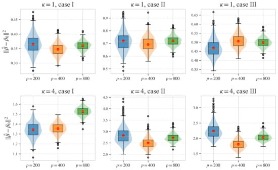
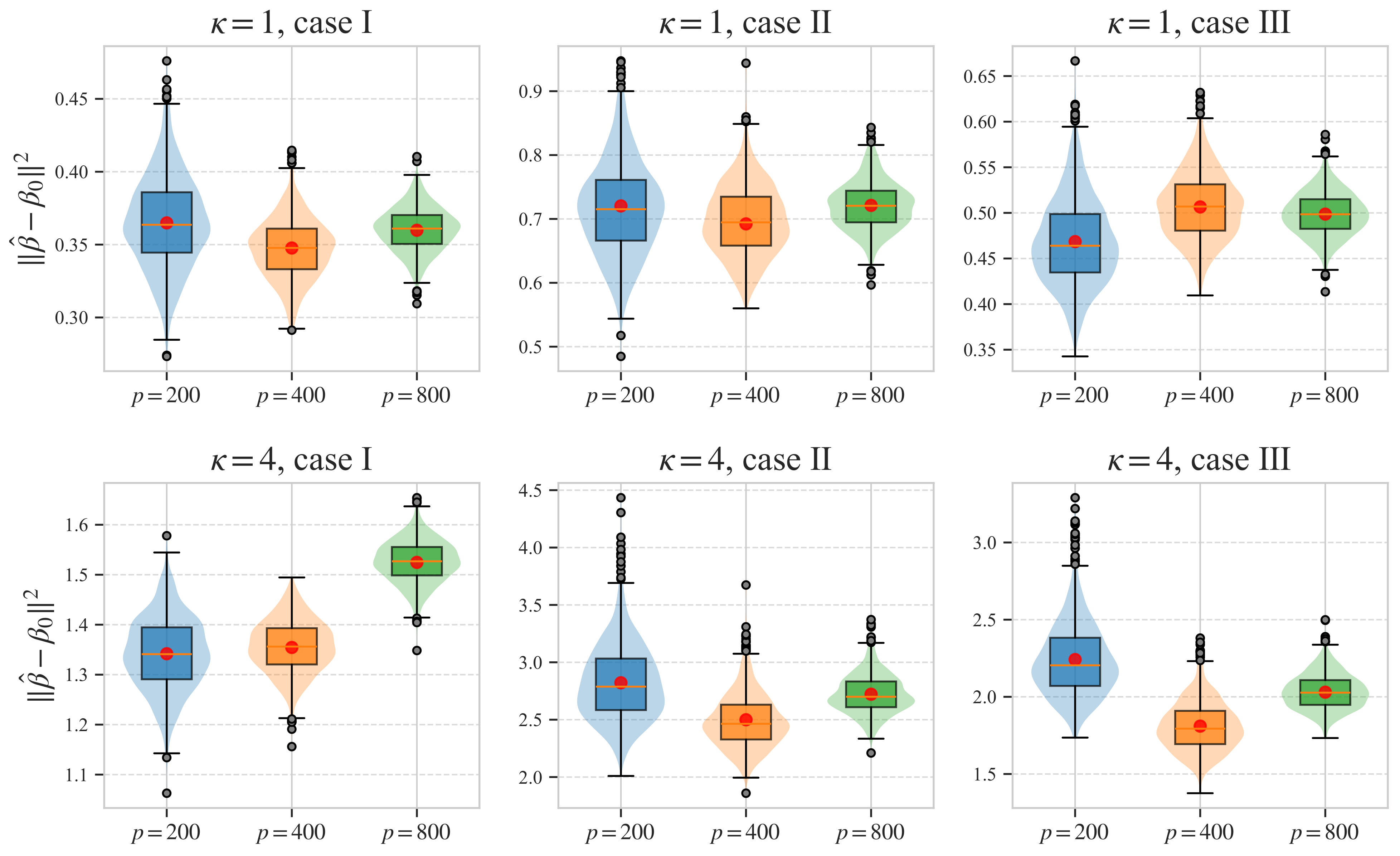
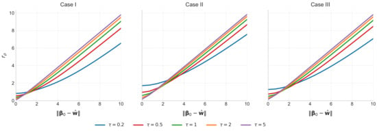
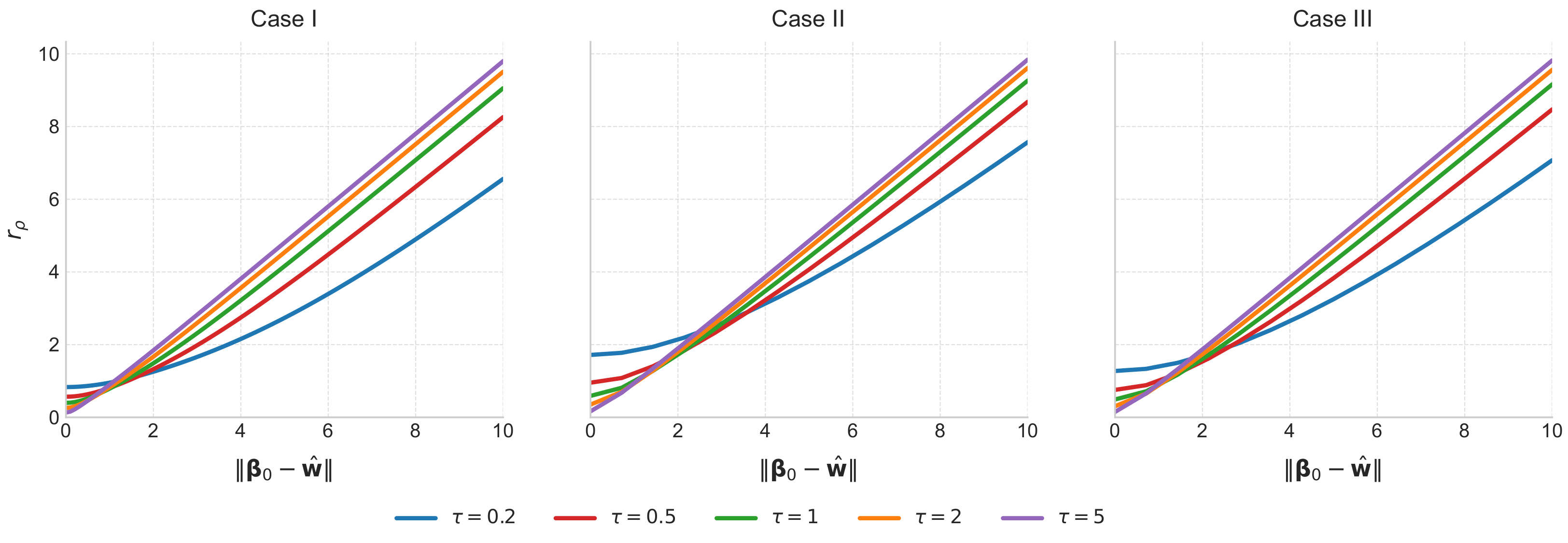
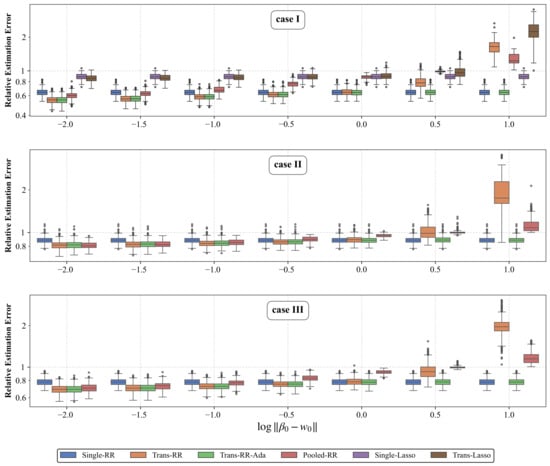
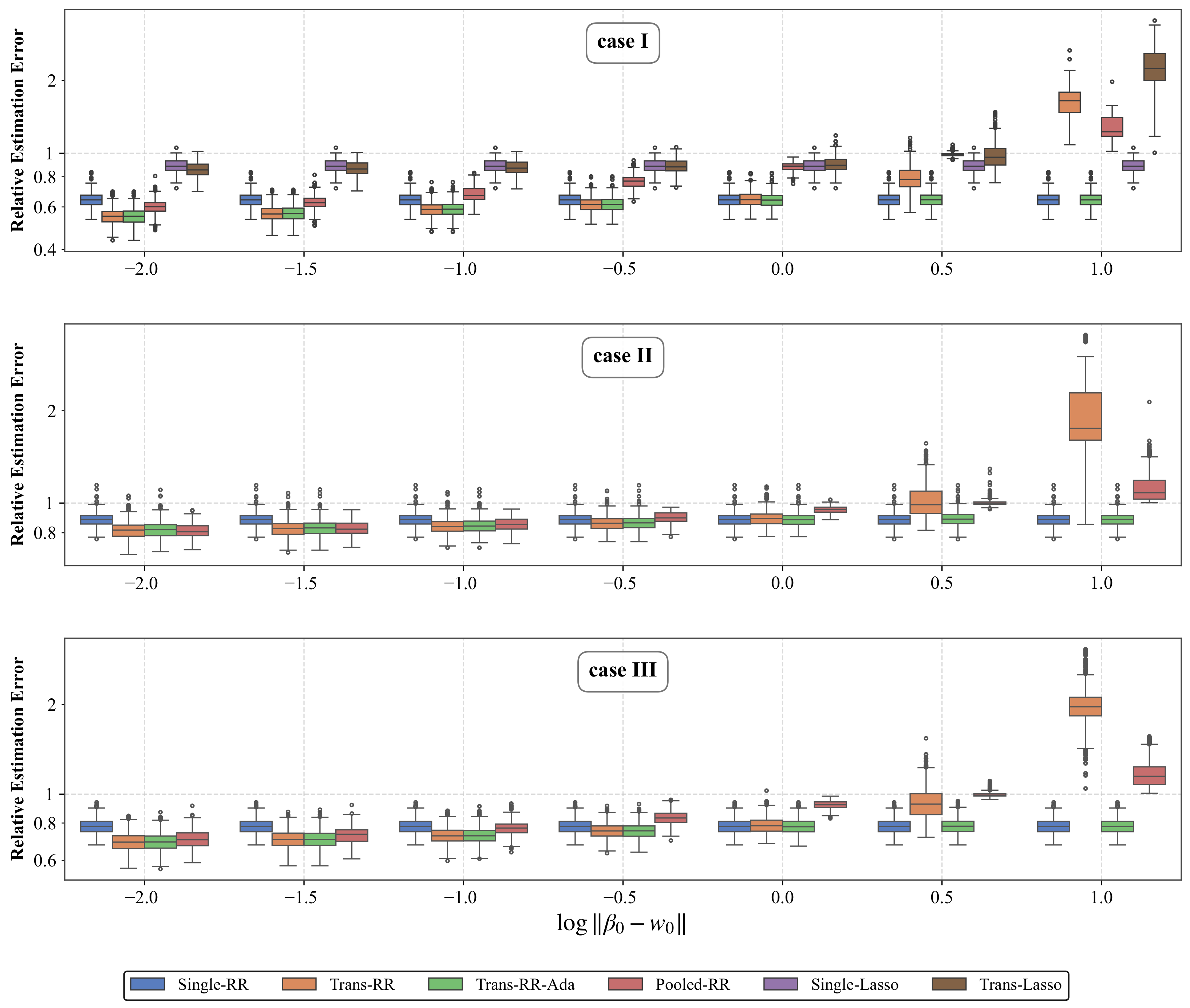
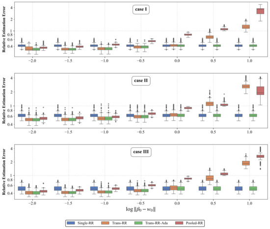
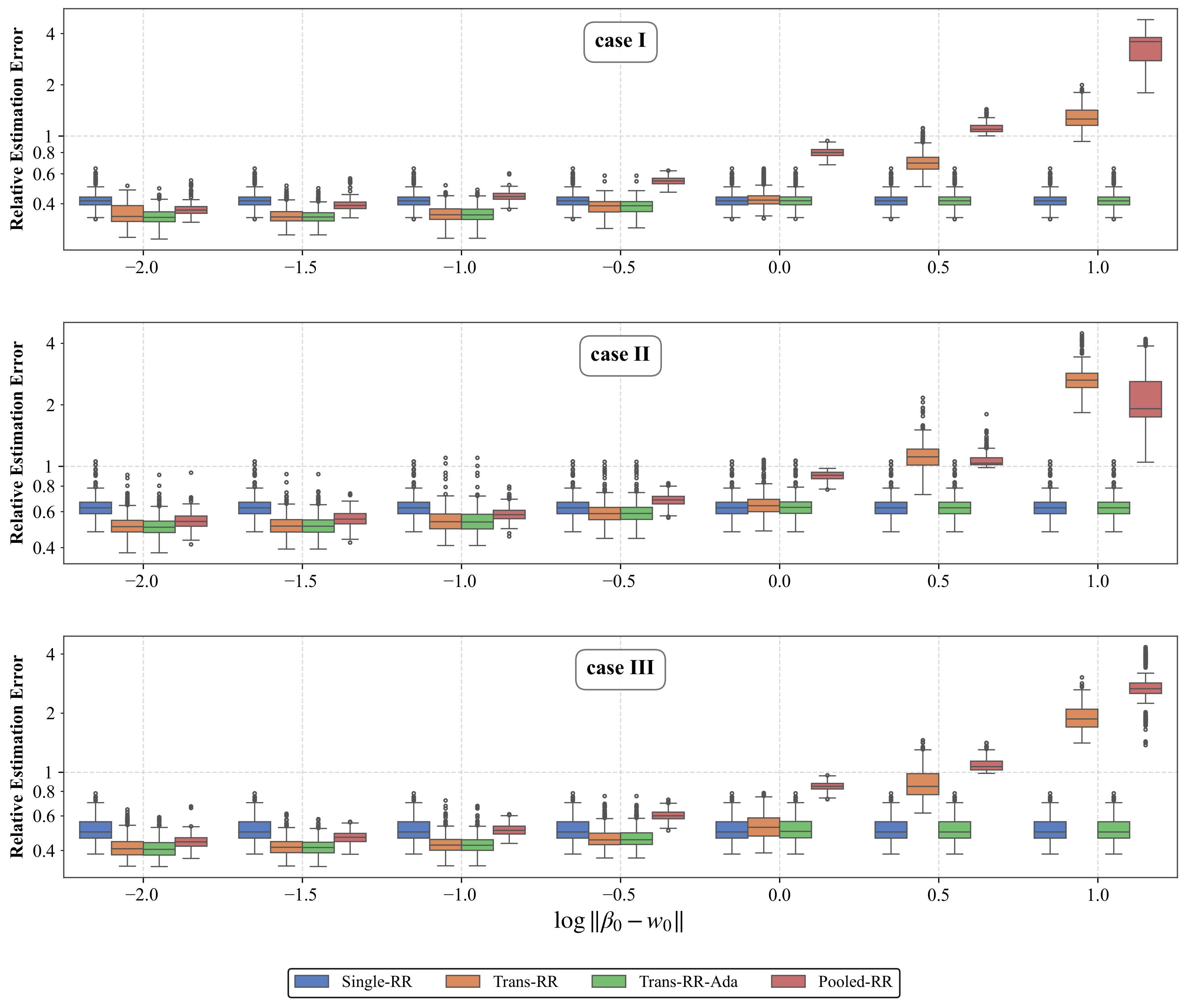
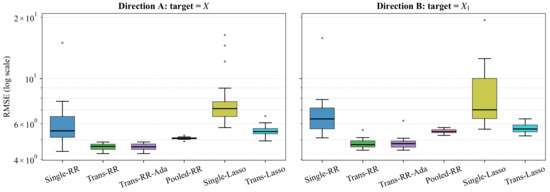
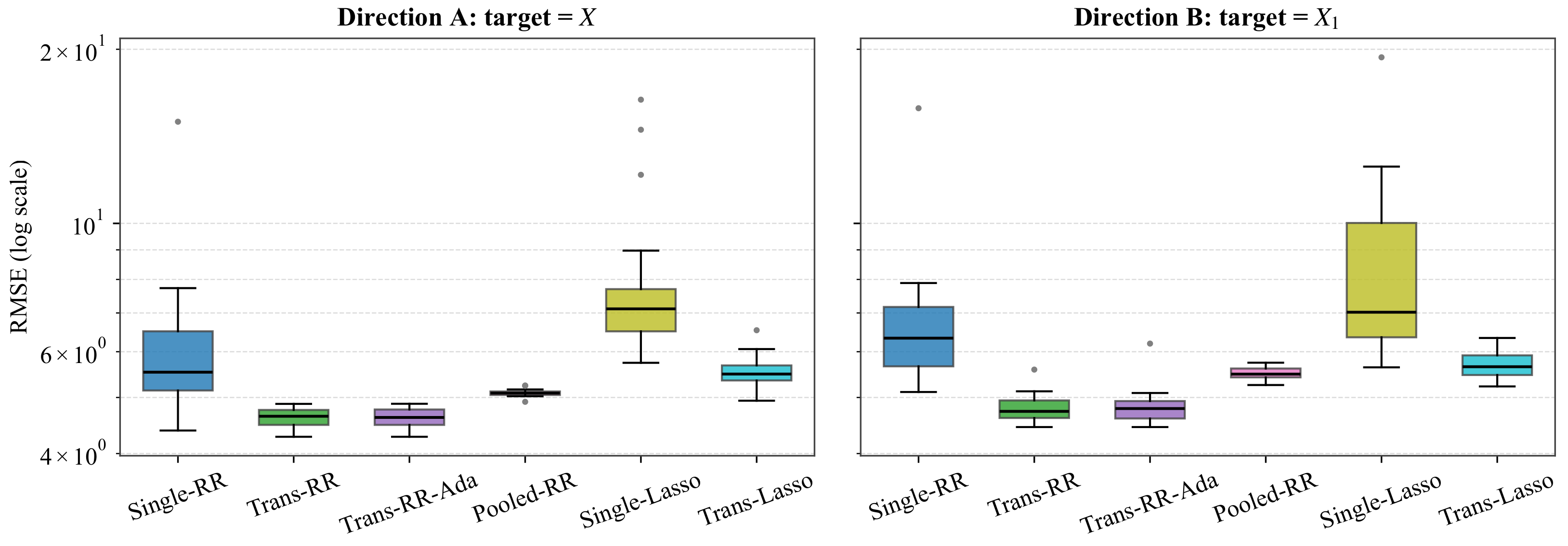

Disclaimer/Publisher’s Note: The statements, opinions and data contained in all publications are solely those of the individual author(s) and contributor(s) and not of MDPI and/or the editor(s). MDPI and/or the editor(s) disclaim responsibility for any injury to people or property resulting from any ideas, methods, instructions or products referred to in the content. |
© 2026 by the authors. Licensee MDPI, Basel, Switzerland. This article is an open access article distributed under the terms and conditions of the Creative Commons Attribution (CC BY) license.