


Abstract
We study Maximum Entropy density estimation on continuous domains under finitely many moment constraints, formulated as the minimization of the Kullback–Leibler divergence with respect to a reference measure. To model uncertainty in empirical moments, constraints are relaxed through convex penalty functions, leading to an infinite-dimensional convex optimization problem over probability densities. The main contribution of this work is a rigorous convex-analytic treatment of such relaxed Maximum Entropy problems in a functional setting, without discretization or smoothness assumptions on the density. Using convex integral functionals and an extension of Fenchel duality, we show that, under mild and explicit qualification conditions, the infinite-dimensional primal problem admits a dual formulation involving only finitely many variables. This reduction can be interpreted as a continuous-domain instance of partially finite convex programming. The resulting dual problem yields explicit primal–dual optimality conditions and characterizes Maximum Entropy solutions in exponential form. The proposed framework unifies exact and relaxed moment constraints, including box and quadratic relaxations, within a single variational formulation, and provides a mathematically sound foundation for relaxed Maximum Entropy methods previously studied mainly in finite or discrete settings. A brief numerical illustration demonstrates the practical tractability of the approach.
1. Introduction
The Maximum Entropy principle provides a classical framework for estimating probability distributions from partial information, typically in the form of moment constraints. In its standard formulation, the problem is posed on a finite or discrete sample space and reduces to a finite-dimensional convex optimization problem, which has been extensively studied in statistics and machine learning.
In many situations of interest, however, the underlying sample space is continuous and no natural discretization is available. Estimating a probability density on a continuous domain under moment constraints then leads to an infinite-dimensional optimization problem, for which the usual finite-dimensional duality arguments no longer apply directly.
Such continuous-domain formulations arise naturally in a variety of applications, including density estimation for physical or environmental variables (e.g., wind or ocean directions, spatial intensity fields), inverse problems and signal processing, and nonparametric statistical modeling where the unknown distribution is supported on a continuum. In directional and circular statistics, for instance, probability densities on the unit circle or sphere are routinely modeled without discretization [1,2]. In these settings, discretization may introduce bias or artificial constraints, whereas a genuine functional formulation is often preferable.
Continuous or nonparametric variants of the Maximum Entropy principle have also been studied in the literature, with foundational contributions by Csiszár on I-divergence geometry and entropy-based inference under exact linear constraints [3,4]. While these works exploit convexity and information-theoretic inequalities to enforce strict moment conditions in a rigorous manner, other continuous-domain treatments proceed in a more formal manner. In many such approaches, the entropy functional and the moment constraints are written in a continuous setting and optimal densities are derived by variational arguments or by analogy with the discrete case. Although these derivations often lead to plausible expressions, the precise functional-analytic framework and the underlying duality structure are frequently left implicit or treated only at a formal level.
Classical treatments of the Maximum Entropy principle in information theory and statistical physics rely on the formal Lagrange multiplier arguments and variational calculus [5,6,7]. In practice, continuous problems are often handled either through discretization or binning strategies that yield finite-dimensional approximations, or via parametric exponential-family models. While frequently effective, such approaches depend on approximation choices that may influence stability and accuracy.
From a convex-analytic perspective, entropy minimization can be formulated within the theory of convex integral functionals [8]. In the discrete setting, Dudík et al. [9] developed a systematic framework for Maximum Entropy estimation with relaxed moment constraints. The present work extends this line of research to genuinely continuous domains, where the primal variable is an infinite-dimensional density.
The purpose of this paper is to provide a fully rigorous formulation of the continuous-domain Maximum Entropy problem. We consider the minimization of the Kullback–Leibler divergence with respect to a reference measure under finitely many (possibly relaxed) moment constraints, where the optimization variable is a probability density defined on a continuous domain. The primary problem is genuinely infinite-dimensional and is formulated in a space of measurable functions defined by integrability with respect to a prescribed family of feature functions.
More precisely, the functional framework is built upon a dual pair of Köthe-type spaces associated with the chosen feature family, allowing moment constraints to be well defined. This setting accommodates a wide range of feature functions, including unbounded ones, and provides a natural domain for entropy optimization.
Our main contribution is to show that, under explicit and mild assumptions ensuring well-posedness of the moment operators and nonemptiness of the relevant effective domains, this infinite-dimensional convex problem admits a dual formulation involving only finitely many variables. The analysis relies on convex integral functionals and an extension of Fenchel duality, and yields precise primal–dual optimality conditions.
The proposed framework is closely related in spirit to the discrete relaxed Maximum Entropy approach of Dudík et al. [9]. It can be viewed as its continuous-domain counterpart, in which the finite-dimensional structure of the dual problem is preserved while the primal variable becomes an infinite-dimensional density.
Since empirical moments are computed from finite samples, they are subject to sampling variability and measurement noise. Enforcing them as exact constraints may therefore lead to overfitting or even infeasibility. This observation motivates the introduction of relaxed constraints through convex penalty functions, which provide a principled way to incorporate uncertainty while retaining the variational structure of the Maximum Entropy principle.
The paper is organized as follows. Section 2 formulates the continuous Maximum Entropy problem and introduces relaxed moment constraints. Section 3 derives the dual problem and establishes primal–dual optimality conditions. Section 4 discusses several choices of relaxation potentials and their consequences for the dual formulation. A brief numerical illustration is presented in Section 5, and concluding remarks are provided in Section 6.
2. Statement of the Problem
We consider the optimization of the so-called differential entropy or its relative counterpart, the Kullback–Leibler divergence between probability measures.
Let be a bounded domain. We assume throughout that is endowed with the -algebra of Borel sets. The space of Borelian functions on is denoted by .
Points are observed in . These points are assumed to be drawn according to some unknown probability P on , and the fundamental problem is that of recovering P. Feature functions are chosen, from which the following statistics are derived:
The functions , also called moment functions, define the moment constraints of the problem.
Recall that the above equation expresses the expectation of under the empirical measure
in which denotes the Dirac measure at . The Maximum Entropy principle states, in its native form, that among all probability measures P that are consistent with the moment constraints
one should select the probability , which minimizes the Kullback–Leibler relative entropy of P with respect to . Here, is a reference measure, supported in , which encodes the prior knowledge one may have about P. If no prior knowledge is available, it is customary to choose to be the uniform measure on . Recall that the Kullback–Leibler relative entropy of P with respect to is defined as
Here, denotes the Radon–Nikodym derivative of P with respect to , and the notation means that P is absolutely continuous with respect to . We are facing the following optimization problem:
The shorthand s.t. stands for subject to, while is the vector whose k-th component equals and is the -valued function whose k-th component equals .
Problem is an infinite-dimensional convex problem with finitely many linear constraints. Although the optimized variable P lies in the space of Radon measures on , it is equivalent to searching for a density with respect to . As a matter of fact, minimizing the Kullback–Leibler divergence discards measures that are not absolutely continuous with respect to .
Since empirical moments are computed from finite samples, they are subject to sampling variability and measurement noise. Enforcing them as exact constraints may therefore lead to overfitting or infeasible formulations; this motivates the introduction of relaxed constraints. Following Ref. [9], we introduce, for the purpose of relaxation, a convex potential function .
We therefore obtain the relaxed, functional counterpart of Problem , namely
in which the variable p is the Radon–Nikodym derivative of the searched measure P with respect to . The neg-entropy functional H is defined by
and the linear operators and are, respectively, defined by
For convenience, we group these linear operators into a single moment operator
which collects the normalization and moment constraints. This notation will be used throughout the sequel. The potential function U is generally a convex non-negative function, which attains its minimum value at . The case of non-relaxed constraint [9] corresponds to the choice . Recall that the indicator function of a set S is the function
Clearly, this choice enforces the equality . In [9], the case of box constraints was also considered. It corresponds to the choice , in which B is box
with . In this finite-dimensional setting, the convex conjugate of coincides with the support function of the set , namely
where the pairing is the standard Euclidean inner product. Since the convex conjugate of fails to be differentiable, one may consider an approximation of the box constraint that yields a differentiable conjugate, as in Section 5.2 of [9]. This will also be considered in the present paper. The least square relaxation corresponds to the choice
in which denotes the Euclidean norm and is some positive constant. We may also consider, more generally, the choice
in which where Q is a positive definite symmetric matrix. An interesting example of this is obtained if we let , with an estimate of the covariance matrix of the vector : the relaxation then accounts for the variance of each principal component of the data vector regarded as a random vector.
Implicitly, the above problem is posed in a space of measurable functions for which all moment constraints are well defined. More precisely, the natural domain of the optimization problem consists of functions that are integrable against the chosen family of feature (moment) functions.
This space is a subspace of , the space of measurable functions that are integrable with respect to the reference measure , and coincides with when all feature functions are bounded. In general, however, it is a proper subspace, since the moment operator is only well defined for densities p such that the pointwise products , defined by , belong to for every .
More generally, for a family of feature functions , the natural workspace of the moment problem is the Köthe dual space
In the next section, we shall explore the dualization of problem and show how this dualization provides algorithms for effective computation of Maximum Entropy solutions in our infinite-dimensional setting, without having to discretize the statistical problem under consideration.
3. Maximum Entropy Solutions
This section derives the dual formulation of the relaxed Maximum Entropy problem. Although the primary variable is an infinite-dimensional density, convex duality allows the problem to be reduced to the optimization of finitely many dual variables (Lagrange multipliers). The analysis relies on standard tools from convex analysis—in particular, convex conjugates, subdifferentials, and Fenchel duality—which provide a natural framework for establishing duality and optimality conditions. Standard references include [10,11,12], while results on convex integral functionals can be found in [8,13,14]. A recent overview in the context of entropy optimization is provided in [15].
For convenience, we define on the concave function
and rewrite in the equivalent form
in which . Here, denotes the composition of functions, that is, . We shall also write with V a proper convex lower semi-continuous (and most often even) function. We note that the dual problem associated with reads
The symbol ★ can denote different, though related, mathematical notions depending on context. When used as a superscript on a function, as in , it typically refers to the convex conjugate (or Legendre–Fenchel transform) of H. When used as a subscript, as in , it denotes the concave conjugate. In the context of linear operators, the same symbol used as a superscript, as in , denotes the adjoint of the operator .
Let us clarify the notion of adjunction being referred to here: in our context, the operator is well-defined from the space with to , and its adjoint is defined with respect to the pairing of with
realized via the standard integral bilinear product
An immediate computation shows that the adjoint of is then given by
We use the notation for the relative interior of a convex set C, that is, the interior taken with respect to the affine hull of C (see [10]).
Theorem 1.
is optimal in problem .
Assume That The Following Conditions Hold:
- (i)
- for every , the function is integrable over every set of finite measure;
- (ii)
- ;
- (iii)
- ;
- (iv)
- the function V underlying the definition of G is closed and proper convex.
- If maximizes the dual function D, then the density defined on Ω by
Proof.
for every , thanks to Equation (5). Replacing by yields (a). Finally, differentiating
through the integral sign shows that
Thus, (b) is also satisfied, and the proof is complete. □
Step 1. By Fenchel duality, thanks to Condition (ii), the optimal value of Problem coincides with that of the dual problem , and dual attainment is achieved:
See, e.g., Theorem 4 of [15].
Step 2. We now turn to the computation of the dual function. We start by computing the concave conjugate of G:
in which the last equality is obtained by the change of variable . Let us now compute the convex conjugate of H in the pairing (4). Condition (i) implies, via Lemma 1 and Proposition 1 [16], that both and are decomposable. Moreover, the entropy kernel is a measurable integrand that is proper convex and lower semi-continuous. Its convex conjugate is provided by
Since is decomposable and H has a nonempty effective domain, it follows that, for every ,
Otherwise expressed, conjugacy through the integral sign holds. Now, since is proper convex and lower semi-continuous. Moreover, it is readily seen that
See Property (f) of [16] (p. 207). It follows that conjugacy through the integral sign applies one more time: for all ,
Step 3. We shall prove here that the dual solution satisfies
- (a)
- ;
- (b)
- has gradient at .
The conclusion then follows from Theorem 6 of [15], since (see Equation (6)) and under Assumption (iv). Clearly, is differentiable throughout , and its derivative equals itself. By integrating the subdifferential inequality as in Proposition 6 of [15], for example, we see that the obvious inclusion gives rise to the following inclusion:
As a byproduct of the above theorem, we see that the dual problem corresponding to Problem consists of maximizing the function
By the first-order optimality condition for concave maximization (often referred to as Fermat’s principle; see [10]), we find that is dual optimal if and only if
Here, the subdifferential is taken in the sense of concavity. Recall that the dual function is concave; thus, sufficiency is granted along with necessity. It is readily checked that the latter condition is equivalent to
in which
Therefore, maximizing the dual function in (7) boils down to maximizing the function . We observe that is concave and upper semi-continuous, as a consequence of the convexity and lower semi-continuity of the log-Laplace transform. We note that evaluating relies on some numerical integration in dimension m. This is by no means a limitation, due to the existence of powerful numerical integration algorithms such as Monte Carlo integration, for example.
Let us summarize the above achievements. If the assumptions of Theorem 1 are satisfied, which clearly depend on the choice of the potential V and on that of the feature functions , we compute the optimal vector by maximizing , and we then obtain the Maximum Entropy solution via the formula
Some potentials V give rise to nice, differentiable, concave-unconstrained maximization problems. This happens whenever the conjugate has a full domain and is differentiable. A standard example is provided by the least square relaxation. However, in general, the function may suffer from drawbacks such as failing to have a full domain (so that the dual problem is constrained) or being non-differentiable. A standard example is provided by the case of box constraints.
In the smooth unconstrained case, quasi-Newtonian methods, such as the BFGS algorithm, are expected to provide a fast and accurate solution. If is not differentiable, the situation can still be addressed using the proximal gradient algorithm. As a matter of fact, in the latter case, the function to be maximized is then a composite concave function, that is to say, a sum of two concave functions, one being differentiable, the other being non-differentiable. The reader interested in the optimization of composite functions and the proximal gradient algorithm may refer to [17,18] and the references therein.
4. Relaxation
Following Ref. [9], we explore a number of potential functions to be used for the reconstruction of multivariate distributions. We assume throughout that the domain of is nonempty—a mild assumption on the family of feature functions.
No relaxation at all. In this case, . The convex conjugate is then the function identically equal to zero. Condition reads in this case, and Condition is automatically satisfied. The reason is that the effective domain of is then the whole of , and that is nonempty, since the relative interior of a nonempty convex set is nonempty.
Box constraints. The function V is defined in this case by
Its convex conjugate is then given by
in which ⊙ denotes the pointwise product. In this case, Condition reads
Condition is, again, automatically satisfied. Since the corresponding function is a composite function, the maximization of will be efficiently performed by the proximal gradient algorithm.
Smoothed inner approximation of box constraints. Let be defined by
The smooth inner approximation of the box constraints with the same box as in the previous paragraph, together with its convex conjugate, are given, respectively, by
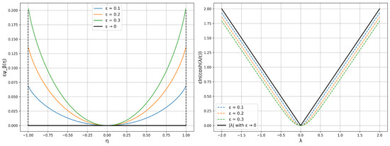
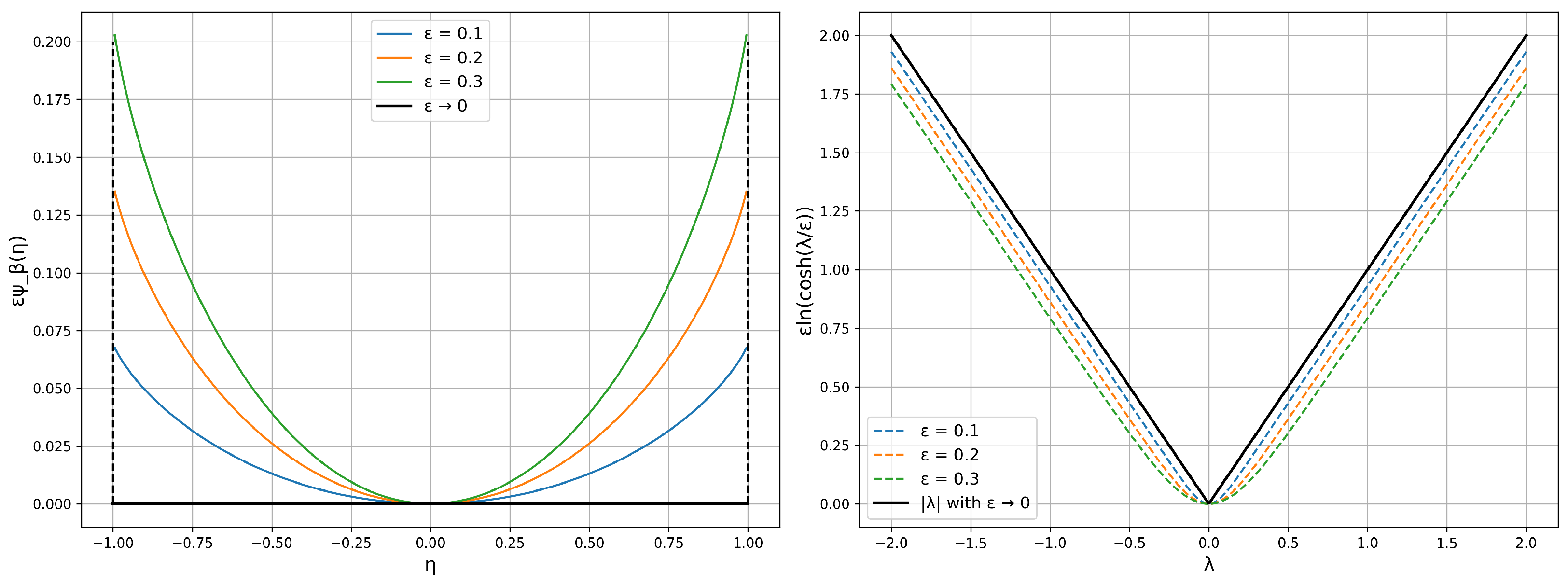
in which controls the proximity of to the target box constraint potential and, thereby, the proximity of the corresponding conjugate functions. Figure 1 illustrates the approximation of the box constraint potential and its conjugate. We note that the constraint qualification condition and its dual counterpart are exactly as in the box constraint case. The advantage here is that the dual function is differentiable, allowing the use of powerful quasi-Newtonian optimization methods.
Figure 1.
Plots of and its conjugate for and various values of .
Least squares. Given a symmetric positive definite matrix Q, the weighted least squares relaxation corresponds to the case where
The standard least squares relaxation is obtained by letting , the identity matrix. If an empirical covariance matrix of the moment vector is available, one may choose . The relaxation term then involves the quadratic form , i.e., a Mahalanobis-type distance. In the eigenbasis of , this amounts to weighting each principal component inversely to its variance, so that directions with larger uncertainty are penalized less strongly.
Remarkably, things once again look nicer on the dual side: no matrix inversion is required to evaluate . Finally, the constraint qualification and its dual counterpart are automatically fulfilled here.
5. Experimental Illustration
This section provides a brief numerical validation of the proposed continuous-domain Maximum Entropy formulation. The goal is not to perform an extensive empirical benchmark, but to illustrate that the dual approach yields stable and meaningful density reconstructions without discretizing the domain. We consider both synthetic data and a real-world meteorological dataset.
5.1. Synthetic Angular Densities
We first consider synthetic directional data on the unit circle, a classical setting in circular statistics. Three target densities are used: a unimodal von Mises distribution, a symmetric bimodal mixture, and a trimodal mixture. For each case, samples are generated.
Densities are reconstructed using trigonometric feature functions
with . A quadratic relaxation is employed, and the resulting finite-dimensional dual problem is solved using a quasi-Newton (BFGS) method. Normalization constants are evaluated by numerical quadrature.
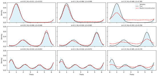
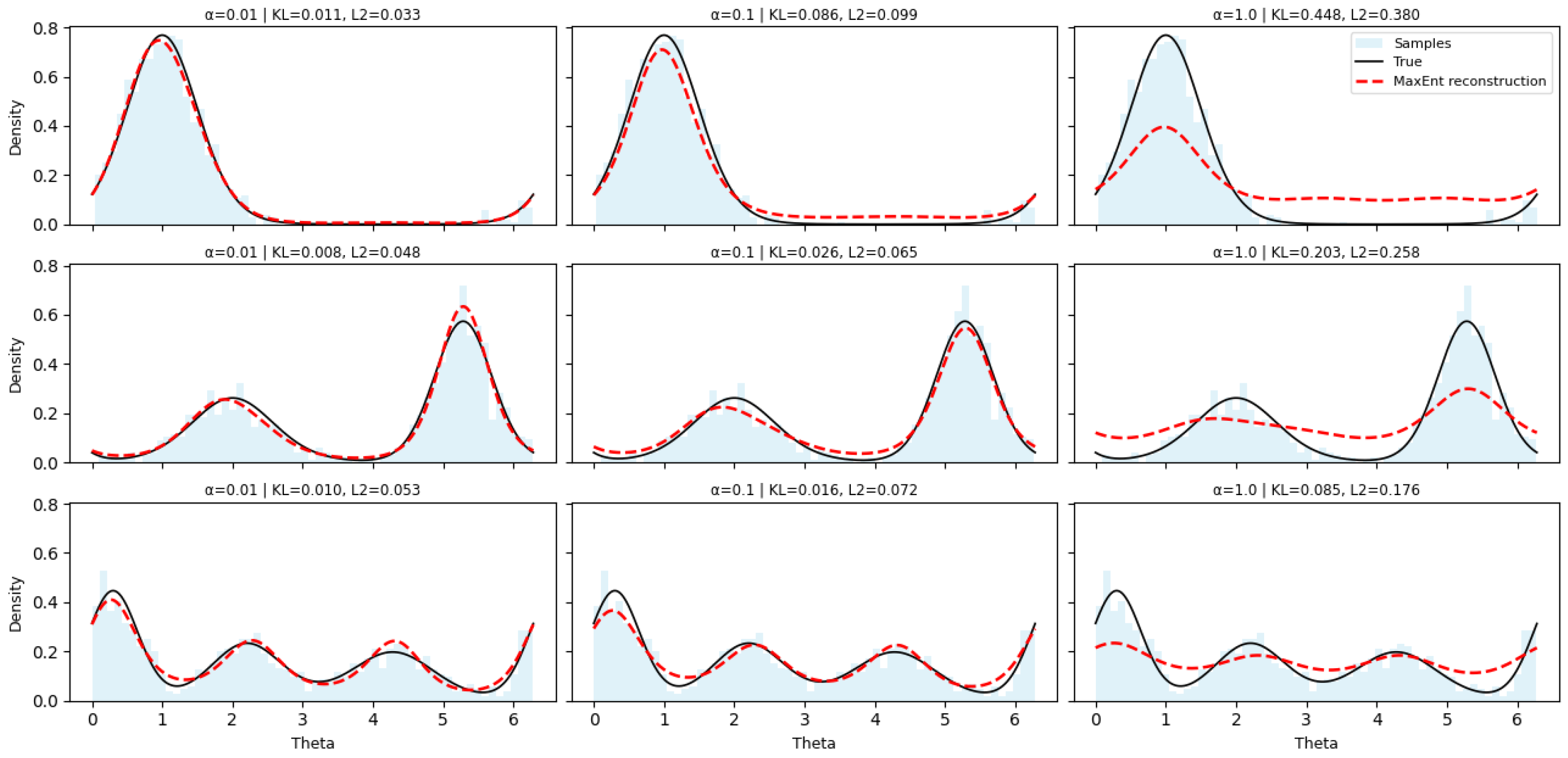
Representative reconstructions are shown in Figure 2. In all cases, the Maximum Entropy solution correctly captures the qualitative structure of the target distribution, including multimodality, without any discretization of the domain. The regularization parameter controls smoothness: small values preserve sharp features, whereas larger values produce smoother densities.
Figure 2.
Reconstructed MaxEnt angular densities for unimodal, bimodal, and trimodal distributions under varying regularization strengths . Each subplot shows the true density (black solid), reconstructed density (red dashed), and sampled histogram (blue). Smaller values preserve sharper peaks and fine directional structure, while larger values yield smoother but less distinct reconstructions.
5.2. Wind Direction Reconstruction
We next evaluate the method on a real meteorological dataset consisting of aircraft-based wind measurements over Europe (January 2018) [19]. The main recorded variables relevant to our study are summarized in Table 1.
Table 1.
Meteorological observation attributes used in the wind direction reconstruction.
The data include horizontal wind components , from which wind directions are computed as
A random subset of observations is used.
As a reference, we compare the proposed Maximum Entropy estimator with a circular kernel density estimate (KDE). Reconstruction quality is assessed using the distance, the Kullback–Leibler divergence, and held-out log-likelihood.
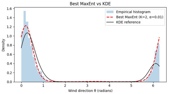
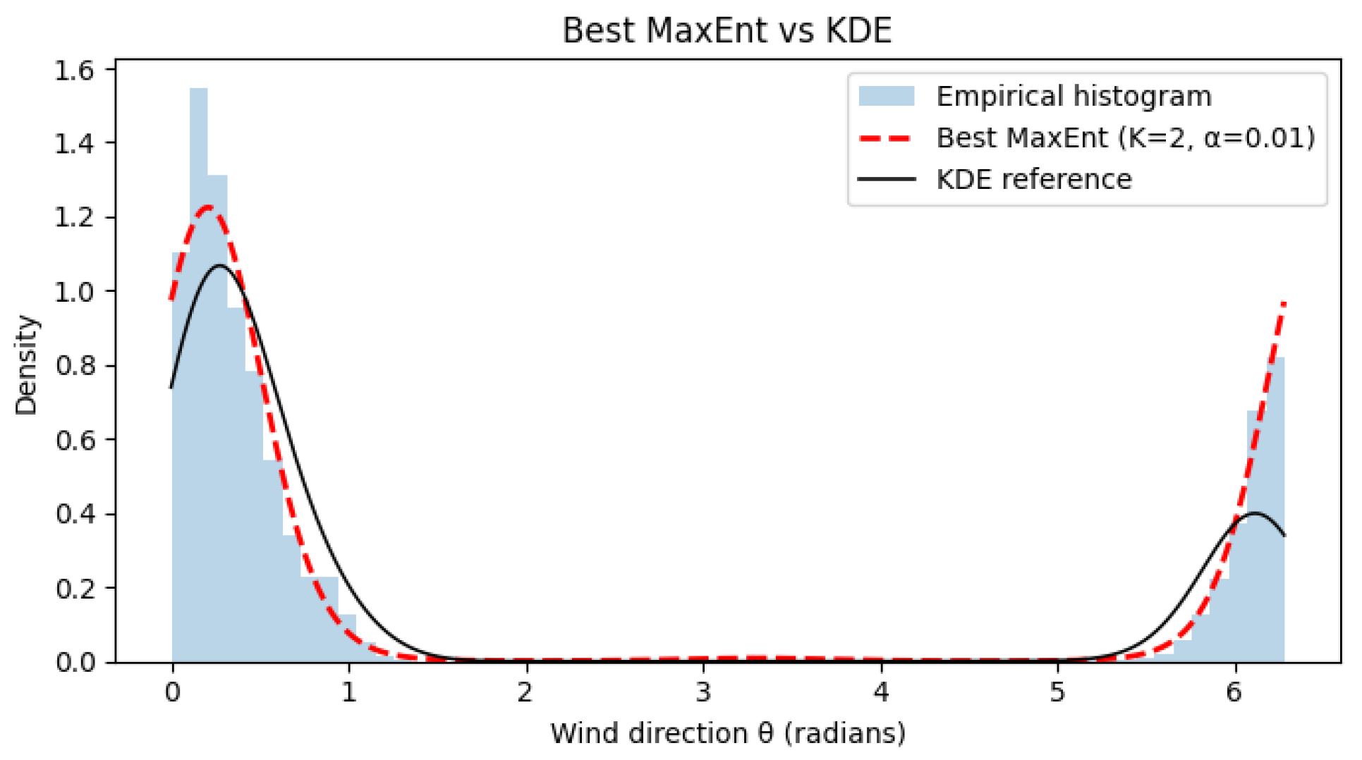
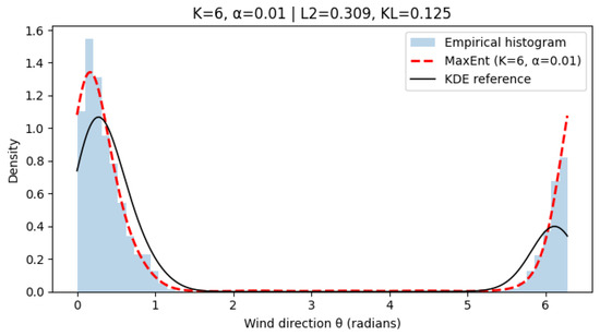
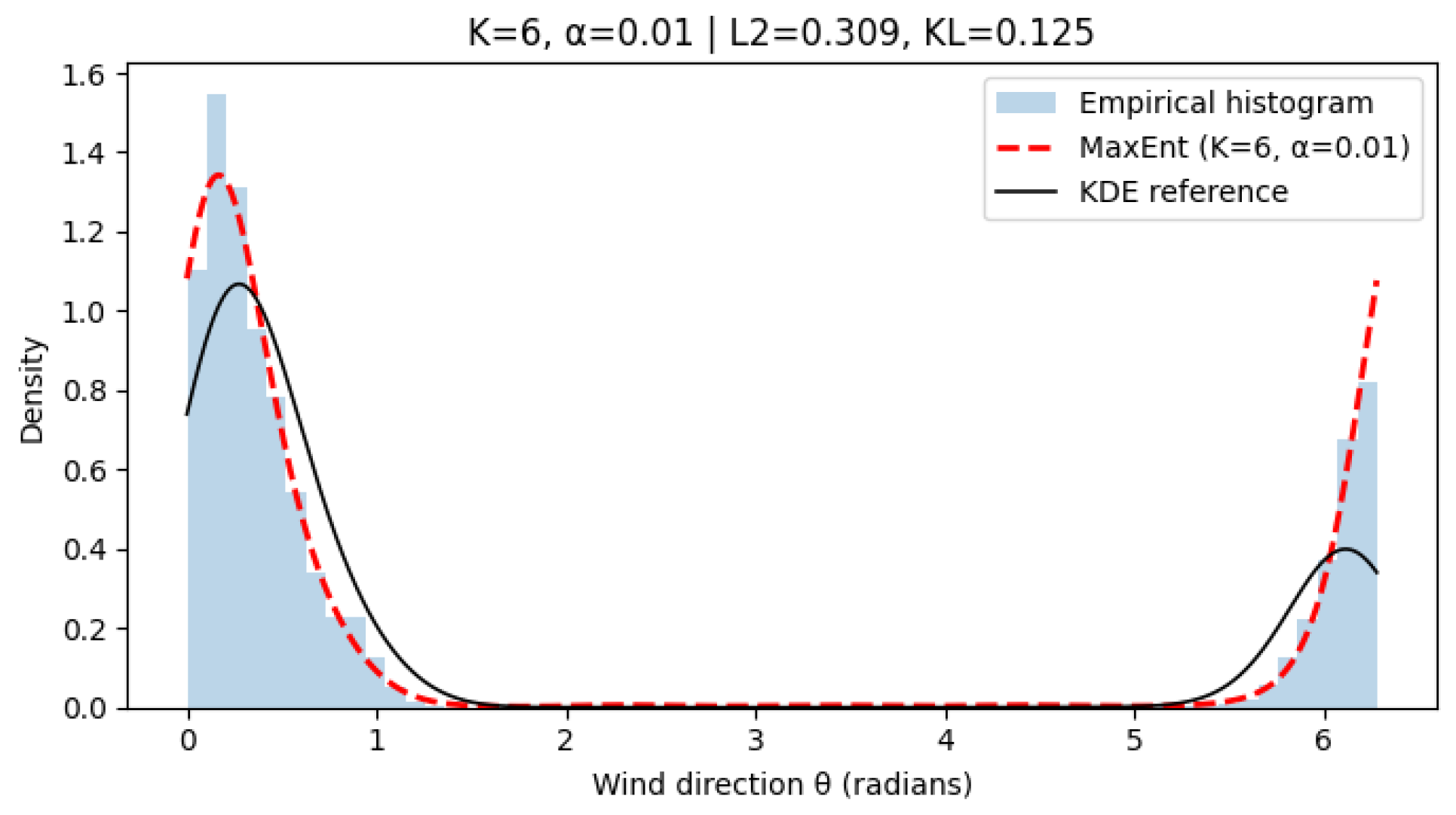
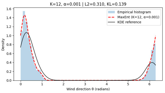
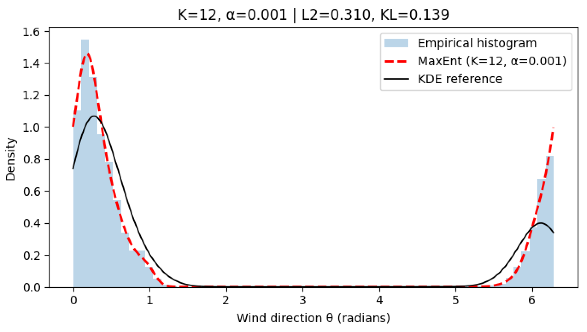
Figure 3, Figure 4 and Figure 5 show representative results for increasing harmonic orders K and different regularization strengths . With few harmonics (), the method already captures the dominant wind regimes. Increasing K improves fidelity, while moderate regularization prevents oscillations. A very small may introduce mild overfitting. Quantitative results in Table 2 confirm that intermediate values (K = 4–6, ) provide the best trade-off between accuracy and smoothness.
Figure 3.
Reconstructed wind direction distribution using MaxEnt with , . The MaxEnt estimate (red dashed) accurately captures the two dominant wind regimes while maintaining smoothness and stability.
Figure 4.
Reconstructed wind direction distribution using MaxEnt with , . The model achieves improved alignment with the KDE reference while preserving numerical stability and smooth transitions.
Figure 5.
Reconstructed wind direction distribution using MaxEnt with , . Increasing model complexity allows for finer detail but may induce small oscillations near modal peaks.
Table 2.
Quantitative comparison between MaxEnt and KDE on wind direction data.
Overall, these experiments illustrate that the proposed continuous-domain formulation produces stable and interpretable density estimates while avoiding discretization or kernel bandwidth tuning.
6. Conclusions
This paper developed a continuous-domain formulation of the Maximum Entropy principle for multivariate density estimation under moment constraints. By combining convex duality with the theory of convex integral functionals, we showed that an infinite-dimensional entropy minimization problem over probability densities admits a finite-dimensional dual representation. This result provides a rigorous and tractable foundation for Maximum Entropy estimation without discretizing the underlying domain.
The introduction of relaxed moment constraints through convex potential functions allows for a unified treatment of exact constraints, box constraints, and quadratic relaxations. On the dual side, this leads to concave optimization problems whose analytical and numerical properties depend explicitly on the chosen relaxation while remaining amenable to standard optimization algorithms.
From a conceptual standpoint, the proposed framework bridges the gap between classical discrete Maximum Entropy formulations and genuinely nonparametric continuous models. It preserves the interpretability and structural simplicity of the entropy principle while extending its applicability to settings where discretization may introduce bias or instability.
The selection of appropriate feature functions remains a central issue in continuous-domain Maximum Entropy modeling and deserves further investigation.
Future work will focus on principled choices of feature families and on extensions to structured domains, including spatial, physically informed, or space–time settings with partial observations.
Author Contributions
Conceptualization, P.M.; methodology, P.M. and T.L.N.; validation, T.L.N.; formal analysis, P.M.; investigation, P.M.; data curation, T.L.N.; writing—original draft preparation, P.M. and T.L.N.; writing—review and editing, P.M. and T.L.N.; visualization, T.L.N.; supervision, P.M. All authors have read and agreed to the published version of the manuscript.
Funding
This research received no external funding.
Data Availability Statement
The data analyzed in this study are publicly available on Figshare at https://doi.org/10.6084/m9.figshare.6970403.v1 [19].
Conflicts of Interest
The authors declare no conflicts of interest.
References
- Fisher, N.I. Statistical Analysis of Circular Data; Cambridge University Press: Cambridge, UK, 1995. [Google Scholar]
- Pewsey, A.; Neuhauser, M.; Ruxton, G. Circular Statistics in R; Oxford University Press: Oxford, UK, 2013. [Google Scholar]
- Csiszár, I. I-divergence geometry of probability distributions and minimization problems. Ann. Probab. 1975, 3, 146–158. [Google Scholar] [CrossRef] [Scilit]
- Csiszár, I. Why least squares and maximum entropy? An axiomatic approach to inference for linear inverse problems. Ann. Stat. 1991, 19, 2032–2066. [Google Scholar] [CrossRef] [Scilit]
- Jaynes, E.T. Information Theory and Statistical Mechanics. Phys. Rev. 1957, 106, 620–630. [Google Scholar] [CrossRef] [Scilit]
- Jaynes, E.T. Probability Theory: The Logic of Science; Cambridge University Press: Cambridge, UK, 2003. [Google Scholar]
- Cover, T.M.; Thomas, J.A. Elements of Information Theory, 2nd ed.; John Wiley & Sons: Hoboken, NJ, USA, 2006. [Google Scholar]
- Rockafellar, R.T. Convex integral functionals and duality. In Contributions to Nonlinear Functional Analysis; Academic Press: Cambridge, MA, USA, 1971; pp. 215–236. [Google Scholar] [CrossRef] [Scilit]
- Dudík, M.; Phillips, S.J.; Schapire, R.E. Maximum entropy density estimation with generalized regularization and an application to species distribution modeling. J. Mach. Learn. Res. 2007, 8, 1217–1260. [Google Scholar]
- Rockafellar, R.T. Convex Analysis; Princeton University Press: Princeton, NJ, USA, 1970; Volume 18. [Google Scholar]
- Hiriart-Urruty, J.B.; Lemaréchal, C. Fundamentals of Convex Analysis; Springer Science & Business Media: Berlin/Heidelberg, Germany, 2004. [Google Scholar]
- Borwein, J.M.; Lewis, A.S. Convex Analysis and Nonlinear Optimization; Springer: Berlin/Heidelberg, Germany, 2006. [Google Scholar]
- Rockafellar, R.T. Integrals which are convex functionals. Pac. J. Math. 1968, 24, 525–539. [Google Scholar] [CrossRef] [Scilit]
- Rockafellar, R.T. Integral functionals, normal integrands and measurable selections. In Nonlinear Operators and the Calculus of Variations: Summer School Held in Bruxelles September 1975; Springer: Berlin/Heidelberg, Germany, 2006; pp. 157–207. [Google Scholar] [CrossRef] [Scilit]
- Maréchal, P. Entropy Optimization. In Convex Optimization. Theory, Algorithms and Applications; Springer: Berlin/Heidelberg, Germany, 2025; pp. 489–523. [Google Scholar] [CrossRef] [Scilit]
- Maréchal, P. A note on entropy optimization. In Approximation, Optimization and Mathematical Economics; Springer: Berlin/Heidelberg, Germany, 2001; pp. 205–211. [Google Scholar] [CrossRef] [Scilit]
- Beck, A. First-Order Methods in Optimization; SIAM-Society for Industrial and Applied Mathematics: Philadelphia, PA, USA, 2017. [Google Scholar]
- Teboulle, M. A simplified view of first order methods for optimization. Math. Program. 2018, 170, 67–96. [Google Scholar] [CrossRef] [Scilit]
- Sun, J.; Vû, H.; Ellerbroek, J.; Hoekstra, J.M. Supplemental dataset for “Weather field reconstruction using aircraft surveillance data and a novel meteo-particle model”. PLoS ONE 2018, 13, e0205029. [Google Scholar] [CrossRef] [PubMed]

Disclaimer/Publisher’s Note: The statements, opinions and data contained in all publications are solely those of the individual author(s) and contributor(s) and not of MDPI and/or the editor(s). MDPI and/or the editor(s) disclaim responsibility for any injury to people or property resulting from any ideas, methods, instructions or products referred to in the content. |
© 2026 by the authors. Licensee MDPI, Basel, Switzerland. This article is an open access article distributed under the terms and conditions of the Creative Commons Attribution (CC BY) license.