


Abstract
Classification of rest versus mental arithmetic in the public EEGMAT dataset is often reported with accuracies of 88–99%. Such results usually come from subject-dependent designs, in which epochs from the same person appear in both training and test sets. This design is often intentional and can be appropriate for within-subject prediction. It becomes misleading, however, when the resulting accuracy is read as evidence that a model will work on unseen subjects. We tested how much of the reported accuracy survives a stricter evaluation. Balancing and augmentation were confined to the training data, test sets kept their natural class ratio, and models were selected on validation data. A multilayer perceptron on 57 simple time-domain features was evaluated under four protocols, with over 1000 trained networks and subject-level confidence intervals. Balancing before splitting gave kappa 0.77–0.88, with 45–47% of test items duplicated in training. A correct random epoch split gave kappa 0.29–0.58, so duplicate contamination explains most of the inflation. Leave-one-subject-out evaluation gave kappa 0.19–0.26 and ROC-AUC 0.66–0.71, which is above chance but modest. The remaining subject-dependent advantage (kappa difference 0.06–0.32) is consistent with subject-identity leakage but does not prove it. To our knowledge, no previous study on EEGMAT has examined this question. Results refer to the available 36-subject pool, not to the general population.
1. Introduction
1.1. Background and Motivation
Electroencephalography (EEG) is one of the most widely used physiological signals for inferring mental state, owing to its high temporal resolution, low cost, and non-invasive acquisition [1]. Among the states of interest, mental stress has received particular attention because of its relevance to occupational health, safety-critical work, and everyday well-being, and because it can be induced reliably under laboratory conditions using mental arithmetic and other cognitive-load paradigms [2]. Reviews of this literature consistently note that reported classification accuracies vary widely across studies, and attribute this variability to differences in electrode montage, stressor type, feature-extraction pipeline, and classifier choice. What such reviews document less consistently, however, is the role of evaluation protocol itself: how the training and test partitions were formed, and in particular whether they were formed at the level of the individual subject or at the level of the individual epoch. Mental arithmetic paradigms such as the one used in EEGMAT mainly elicit cognitive engagement and workload; the dataset does not measure stress, and the word “stress” is used below only when citing studies that adopt that label. The two classes analysed in this paper are therefore rest and mental arithmetic task.
Entropy-based and information-theoretic descriptors have played a growing role in this literature, both as classification features and as interpretability tools. Multi-domain transfer entropy has been combined with learned feature representations for EEG-based stress-state classification [2]; network-theoretic entropy measures derived from visibility-graph representations of EEG have been used for cross-subject emotion recognition [3]; and permutation entropy has been used not only as a classification feature but explicitly as an interpretability signal for convolutional neural network (CNN) models applied to EEG, quantifying how the complexity of learned feature maps relates to class-discriminative information [4]. This body of work establishes entropy and mutual information concepts as a natural, already-adopted vocabulary for describing what an EEG classifier has and has not captured. The vocabulary this paper adopts describes a different problem: how much of a classifier’s apparent success reflects a confound rather than a task-related physiological signal, and what confusion-matrix-based information measures can and cannot reveal about it.
1.2. Information Leakage as a Confound in Machine-Learning-Based Science
Data leakage, broadly the unintentional availability of information at evaluation time that would not be available at deployment time, has been identified as a pervasive and under-reported source of overoptimistic results across the quantitative sciences. An early and influential taxonomy distinguished several concrete leakage mechanisms in applied data mining practice, including leakage through non-independent train/test construction [5]. A more recent systematic survey found leakage-related reproducibility problems in at least 294 papers spanning 17 scientific fields, proposing an eight-category taxonomy spanning simple train/test contamination through more subtle forms such as non-independence between nominally separate samples [6]. Framed information-theoretically, leakage of this kind can be understood as the unintended introduction of a confounding variable that is correlated with both the input features and the partition assignment, so that a model’s apparent held-out performance reflects information shared with that confound rather than information shared with the label of scientific interest. A candidate confounding variable of this kind is subject identity: because EEG signals carry strong, stable subject-specific characteristics, a classifier evaluated on epochs from a subject already seen in training may exploit who the recording came from instead of the task-related signal. This is distinct from cross-subject generalization (Section 2.4); lower performance on unseen participants is expected from normal inter-individual variability of EEG amplitude, oscillatory characteristics and task-related responses, and does not by itself indicate leakage.
Whether a train/test construction counts as leakage, however, depends on the scientific question. When the aim is a model for previously unseen individuals, subject-independent validation is required. When the aim is to characterize within-subject neural changes between conditions, training and testing on independent data of the same participants is a legitimate design [7,8,9,10]. What matters then is that dependent samples, such as neighbouring epochs of one recording or duplicated and augmented copies of the same epoch, are not placed on both sides of the split [7,11]. We therefore treat subject-dependent and subject-independent evaluation as two distinct questions and measure how the answer changes with the question, instead of declaring one of them invalid.
Class-imbalance correction compounds this risk when applied without regard to the evaluation protocol. Reviews of imbalance-handling methods in biomedical machine learning generally recommend either synthetic oversampling (e.g., SMOTE-style interpolation) or learned oversampling integrated with the classifier itself, and report that appropriately validated oversampling substantially improves minority-class recall without the accuracy inflation associated with naive duplication [12]. In the EEG literature specifically, both classical statistical perturbation and lightweight, deep-learning-oriented augmentation strategies (additive noise, amplitude scaling and time-shifting) have been shown to improve classification robustness on highly imbalanced EEG datasets, including in explicitly leakage-conscious settings where augmentation is applied strictly within the training partition [13,14]. These studies motivate, but do not by themselves resolve, the question this paper investigates directly: whether a genuine (non-duplicating) augmentation strategy yields a materially different and more defensible estimate of classifier performance than duplicate-based balancing, and, if so, under which of the two evaluation protocols (subject-dependent or subject-independent) that difference matters. Any such balancing or augmentation must be performed inside the training partition after the split; applied before it, duplicates or augmented copies of one epoch land on both sides of the split and inflate the test score irrespective of subject identity.
1.3. The EEGMAT Dataset and Related Mental Arithmetic Studies
The EEGMAT dataset, introduced as a PhysioNet resource pairing resting-state and mental arithmetic task EEG recordings from 36 subjects divided into “good counter” and “bad counter” performance groups (26 and 10 subjects, respectively, according to the subject-information file, but 24 and 12 according to the dataset description; see Section 2.1), has become a recurring benchmark for stress and cognitive-workload classification research [15]. Using this dataset together with paired electrocardiogram (ECG) recordings, multimodal stress classification combining variational mode decomposition with machine learning has been demonstrated, including a duplication-based strategy for balancing the good counter/bad counter class split that this paper explicitly revisits in Section 2.5 [16]. Most published EEGMAT classification work reports accuracies in the low-to-high 90s using windowed, randomly split evaluation, a protocol that by construction allows windows from the same participant to appear in both train and test partitions, including entropy- and mutual information-guided deep recurrent architectures reaching up to 99.72% [17], stacked LSTM networks reaching around 93% [18], and entropy- or rhythm energy-based classifiers in the low-to-high 90s [19,20,21]. Substantially fewer studies evaluate under a genuinely subject-independent (leave-one-subject-out) protocol; the strongest recent point of comparison combines empirical mode-decomposition sub-band features with a random forest and explainable-AI post-hoc analysis, reporting 98.17 ± 0.47% (rest vs. calculation) and 97.19 ± 0.95% (good vs. bad counter) under leave-one-subject-out, compared with 99.30%/98.33% under a subject-dependent split on the same pipeline [22]. A related quantum pattern and triangle-pooling feature pipeline has also been evaluated on the good vs. bad counter distinction under leave-one-subject-out [23]. These subject-independent studies use substantially richer, spectrally and structurally derived feature sets than the three time-domain statistics per channel used here, which is a large part of why the subject-independent performance in Section 3 remains below theirs. Because the dataset offers only 36 subjects, and because the “good counter” and “bad counter” subsets are themselves imbalanced, subject-level correlations of the kind described in Section 1.2 are easy to introduce inadvertently through ordinary epoch-level splitting, making EEGMAT a tractable and instructive case study for quantifying, rather than merely warning about, the scale of protocol-driven inflation in a widely reused public dataset. To our knowledge, no previous work on this dataset has examined how the construction of the training and test partitions affects the reported performance, which is the subject of the present paper.
1.4. Explainability and Information-Theoretic Interpretation of EEG Classifiers
SHAP (SHapley Additive exPlanations), grounded in the cooperative game-theoretic Shapley value, decomposes a model’s output into per-feature contributions that sum exactly to the difference between the model’s output and its expected baseline output, and has become one of the most widely adopted feature-attribution methods for tabular and biomedical classifiers [24]. A recent systematic review of explainable-AI techniques applied to quantitative biomedical prediction tasks found SHAP used in the large majority of surveyed studies, while also noting that computational feature-importance evaluation is rarely accompanied by structured validation against domain knowledge or human-subject usability testing, a gap this paper’s SHAP analysis (Section 3.10) partially addresses by quantifying, rather than merely inspecting, how evenly the retained subject-independent signal is distributed across features and channels [25,26]. Within EEG research specifically, permutation entropy has been used to interpret which learned CNN feature maps drive a clinical EEG classification decision [4], and mutual information-guided feature selection has supported cross-subject generalization in EEG-based affective computing, again illustrating the close, pre-existing relationship between information-theoretic tools and explainability in this literature [3].
1.5. Domain-Informed and Entropy-Consistent Neural Network Design
A complementary strand of the authors’ own research programme has focused on embedding structured domain knowledge directly into neural network architecture and training, rather than treating the network as a purely data-driven black box. Quality-Informed Neural Networks (QINN) translate the relationship matrices of a Quality Function Deployment House of Quality into structural sparsity masks and initialization targets for a classification network, yielding named, auditable hidden units and, in a proof-of-concept classification task distinguishing AI-enabled from classical software components, cross-validated performance that exceeds both a non-learned scoring baseline and a conventional ensemble classifier, while producing interpretability directly aligned with regulatory documentation requirements [27]. In a separate line of work applying spiking neural network principles to mental health-relevant signal classification, a CNN to spiking neural network (SNN) conversion pipeline was developed and evaluated on the DAIC-WOZ depression interview dataset, demonstrating that biologically inspired, information-efficient architectures are a viable alternative to conventional deep networks for mental-state classification from behavioural and physiological signal data [28]. Both lines of work share this paper’s underlying premise that a classifier’s reported performance is only as trustworthy as the structural and evaluative assumptions built into its training and validation pipeline, and that this trustworthiness should be demonstrated rather than assumed. Here, through the weight-entropy and capacity-utilization diagnostics of Section 3.9, which ask not only how well a network performs but how much of its structural capacity that performance actually required.
1.6. Contributions of This Work
We re-examine, in a single controlled design, how much of the very high EEGMAT rest-versus-mental-arithmetic accuracy reported with random epoch-level splits survives when class balancing and augmentation are confined to the training partition, the evaluation protocol is varied systematically between subject-dependent and subject-independent designs, model selection uses a validation set rather than the final training epoch, and uncertainty is quantified with repeated splits and subject-cluster bootstrap confidence intervals. The classifier is a multilayer perceptron (MLP) on per-channel time-domain statistics (mean, standard deviation and skewness). We make no claim that one evaluation protocol is intrinsically correct; each protocol answers a different question (Section 2.4), and we quantify how much the answer changes with the question.
Four evaluation protocols are crossed with nine dataset-construction modes (three subject pools, each with raw, duplicate-balanced and augmented training sets), giving 36 conditions that are repeated many times (1000+ trained networks in the main grid). Two protocols are subject-dependent (random epoch split and within-subject chronologically blocked split) and two are subject-independent (leave-one-subject-out and repeated grouped 80/20 splits).
We add a control that reproduces the order of operations of the existing literature (balance first, split afterwards) and measure how many test items have a duplicate or an augmented copy of their own source epoch in the training partition. This isolates conventional duplicate contamination from subject dependence.
We compute label entropy, mutual information, normalized transfer, normalized and adjusted mutual information and confusion entropy [29] directly from the pooled confusion matrices, and report cross-entropy dynamics, weight-matrix spectral entropy [30] and SHAP explanation entropy [24,31,32] for the same models. We benchmark the results against the published EEGMAT literature (Section 3.12).
Originality and scope. To our knowledge, no previous study on the EEGMAT dataset has systematically examined how the construction of training and test partitions (the order of balancing and splitting, subject-dependent versus subject-independent protocols, the model selection rule) affects the reported performance, nor separated duplicate contamination from subject dependence on this dataset. The paper does not propose a new classifier or a new physiological finding; its contribution is a controlled, quantitative evaluation study with a reusable design (four protocols, a contamination control that counts the test items that have a copy in the training data, subject-cluster bootstrap and per-subject tests) that can be applied to other EEG datasets.
2. Materials and Methods
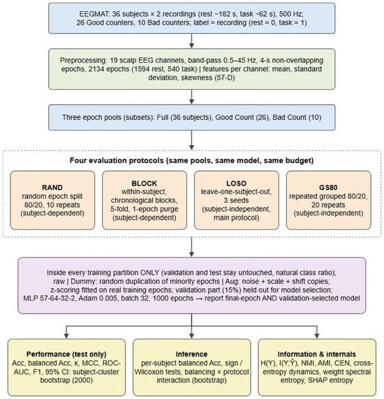
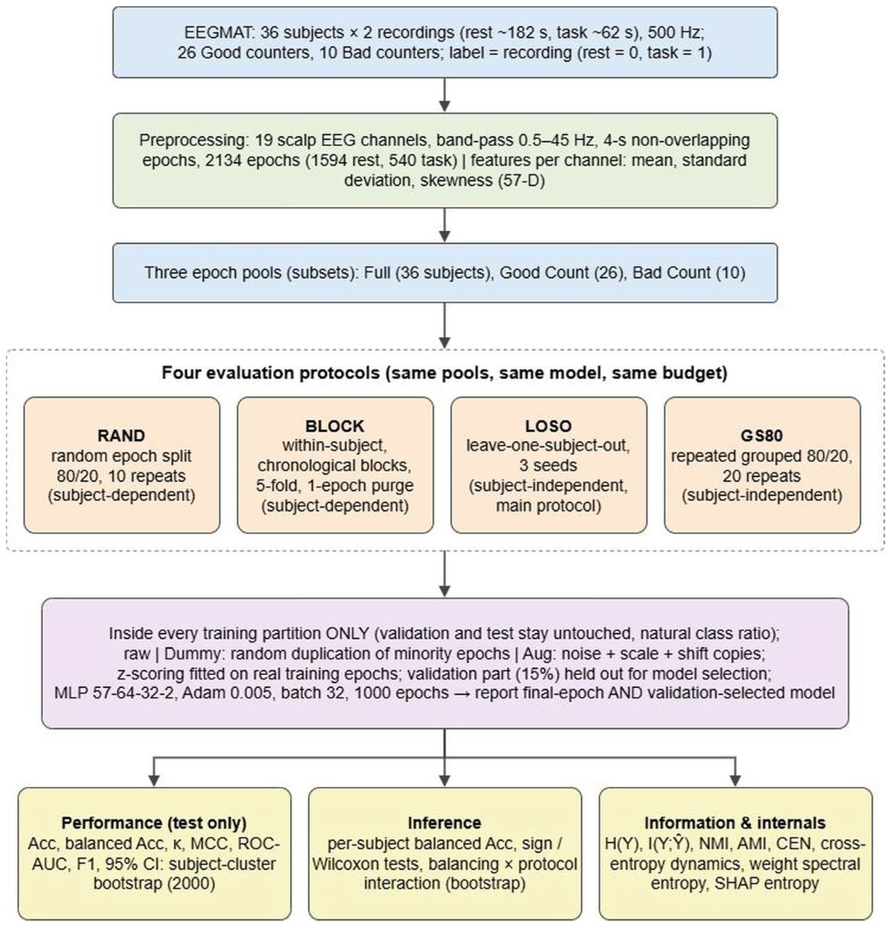
Figure 1 is a map of the experimental design, where all pools, protocols and training-set modes use the same network, optimizer and training budget; balancing and augmentation act on training partitions only; and every test partition keeps the natural class ratio and contains real epochs only.
Figure 1.
Map of the experimental design.
2.1. Dataset
The EEGMAT dataset [15] is a publicly available PhysioNet resource containing EEG recordings from 36 healthy volunteers (students at the Educational and Scientific Centre “Institute of Biology and Medicine”, Taras Shevchenko National University of Kyiv) performing a serial mental subtraction task. For each subject, two recordings are provided: a resting-state background recording (eyes closed, no task; 182 s for 33 subjects, 170, 188 and 80 s for the remaining three) and a recording during the arithmetic task (62 s for all subjects). EEG was acquired with a monopolar Neurocom system (XAI-MEDICA, Ukraine) following the International 10–20 electrode placement system, sampled at 500 Hz, and distributed in EDF format after independent-component-based artifact removal by the data providers. Based on the number of subtractions performed in the task, subjects were divided by the data providers into a “good counter” and a “bad counter” group. The two sources distributed with the dataset differ on the group sizes: the dataset description (README) reports 24 good counters (mean 21 subtractions per 4 min, SD 7.4) and 12 bad counters (mean 7, SD 3.6), whereas the per-subject field count quality of the subject-information file marked 26 subjects as good counters (mean 22.0, SD 7.5; 11.6 to 34.6 subtractions) and 10 as bad counters (mean 6.2, SD 3.4; 1 to 10 subtractions). We could not reconcile the two descriptions, which differ by two subjects, and we used the per-subject labels of the subject-information file because they are explicit, machine-readable and cleanly separated by the number of subtractions (every good counter above 11.5 and every bad counter at most 10). The Full pool results do not depend on this choice; the Good Count and Bad Count pools would each change by two subjects under the alternative grouping (Section 4.4). We refer to these two subject subsets as the Good Count and Bad Count conditions, and to the pooled set of all 36 subjects as the Full condition. Each EDF file contains 21 channels: the 19 scalp EEG leads (Fp1, Fp2, F3, F4, F7, F8, T3, T4, C3, C4, T5, T6, P3, P4, O1, O2, Fz, Cz, Pz), a bipolar A2-A1 channel and an ECG channel. The present analysis uses the 19 scalp leads only, and the 21-channel configuration is retained as an ablation (Section 3.11).
Nature of the contrast. EEGMAT was designed to capture changes of the EEG during mental arithmetic (the data providers analysed spectral power, coherence and fractal measures [15]). The contrast is therefore rest versus cognitive engagement and workload, not a validated stress induction. We name the classes “rest” (Y = 0) and “task” (Y = 1) and use the word “stress” only when referring to prior studies that use it.
2.2. Signal Preprocessing, Task Definition and Labelling
EEG recordings were read and processed in Python using MNE-Python v 1.12.1. Each continuous recording was band-pass filtered between 0.5 and 45 Hz using MNE-Python’s default FIR filter design, and was then segmented into non-overlapping, contiguous 4 s epochs (2000 samples at 500 Hz). Class labels were assigned at the recording level: epochs from a subject’s resting recording were labelled rest (Y = 0) and epochs from the corresponding arithmetic task recording were labelled task (Y = 1); no performance-based sub-segmentation was applied. This yields 2134 epochs (1594 rest, 540 task; task prevalence 0.25), of which 1535 come from good counter subjects (prevalence 0.25) and 599 from bad counter subjects (prevalence 0.25). The natural class imbalance is therefore about 3:1 because the resting recordings are about three times longer than the task recordings. Because every subject contributes exactly one recording per class, the label is perfectly confounded with the recording, a fact that matters for the interpretation of within-subject designs.
2.3. Feature Extraction: Time-Domain Per-Channel Statistics
For each of the 19 channels c and each 4 s, N = 2000 sample epoch, three summary statistics were computed: the mean (µ), the standard deviation (σ) and the skewness (γ) (third standardized moment [33]):
where xc[n] is the n-th sample of channel c within the epoch. These statistics, concatenated across the 19 channels, form a 57-dimensional feature vector per epoch, deliberately minimal (no spectral, connectivity or entropy features), so that any signal recovered can be attributed to simple amplitude-distribution statistics. The root mean square (RMS) was not used as third feature, as it is not an independent dimension: for each epoch exactly (numerically, on all 2134 × 21 initial epoch-channel pairs, the largest deviation was 0.008 µV2). Using the three-feature set (µ, σ, RMS) would span only a two-dimensional space per channel. We replaced RMS by the next statistic in the series of moments, the skewness γc, which is invariant to amplitude scaling and carries information about the shape of the amplitude distribution that the first two moments do not. The original feature set (µ, σ, RMS) is kept as an ablation (Section 3.11). Prior to model input, features were standardized to zero mean and unit variance (z-score) using a scaler fitted on the real training epochs of each split only and applied unchanged to the validation and test epochs.
2.4. Evaluation Protocols
The appropriate validation strategy depends on the scientific question, and random epoch-level splits are legitimate when the goal is to characterize within-subject neural change. Two families are compared. Subject-dependent protocols train and test on data from the same participants and answer the question “can this model recognise the state in a person it has already seen?”. Subject-independent protocols never place a test participant in the training set and answer “can this model recognise the state in a new person?”. We evaluate four protocols with the same network, optimizer and budget.
RAND (random epoch split). Epoch feature vectors of the pool were split at random into 80% training and 20% test epochs, stratified by class and without regard to subject or time (10 independent repetitions; 15% of the training epochs, stratified, form the validation set). This is the design used by most published EEGMAT classifiers. Adjacent 4 s epochs of one recording are strongly autocorrelated, so this protocol measures recall of recording-specific patterns in addition to any state-related signal.
BLOCK (within-subject, chronologically blocked split). For every subject and recording, the epochs were ordered in time and divided into five contiguous blocks; in fold k, block k of every recording formed the test set, epochs adjacent to the test block (one epoch, 4 s, on each side) were purged, and the last 15% of the remaining epochs of each recording (again with a one-epoch purge) formed the validation set. Training and test data therefore come from the same participants but never from neighbouring time points. This is the subject-dependent design that respects temporal dependence.
LOSO (leave-one-subject-out). Each subject in turn forms the test set (both of that subject’s recordings); about 15% of the remaining subjects (at least two) form the validation set and the rest the training set. The procedure was repeated with three different random validation subjects and network initializations. LOSO is the main subject-independent protocol: every subject is tested exactly once per seed and every test set contains both classes.
GS80 (repeated grouped 80/20 split). The design of the original submission (a subject-grouped 80/20 split, scikit-learn GroupShuffleSplit) but repeated 20 times with different random test subjects (7, 5 and 2 test subjects for the Full, Good Count and Bad Count pools), instead of a single split with a single seed. GS80 quantifies how much a single grouped split can mislead.
The test partitions of RAND, BLOCK, LOSO and GS80 always keep the natural class ratio of the pool and contain only real epochs. In LOSO and GS80 each test subject contributes both a resting and a task recording, so the test class ratio is about 3:1 in every fold, instead of the strongly varying ratios (prevalence 0.04 to 0.59) of the single grouped split in the original submission.
Terminology. We distinguish three notions that are often conflated. Contamination: the same epoch, or a copy of it, appears in the training and in the test data. Subject-identity leakage: a model uses subject-specific information that is unrelated to the task to predict the label of a test sample of a subject that was seen in training. Cross-subject generalization gap: the lower performance on unseen participants, which can arise from normal inter-individual variability in EEG amplitude, oscillatory characteristics and task-related responses without any leakage. Comparing the subject-dependent protocols (RAND, BLOCK) with the subject-independent ones (LOSO, GS80) measures the difference between subject-dependent and subject-independent performance. We call this difference the subject-dependent advantage and discuss what it does and does not show in Section 4.1.
2.5. Training-Set Construction and Class Balancing
Within each protocol, three training-set modes were evaluated for each of the three subject pools (Full, Good Count, Bad Count): raw (native class ratio), “Dummy” duplicate-based balancing, and noise/scale/shift augmentation. The rest class is the majority class in every pool, so the minority (task) class is enlarged until the two classes have equal size in the training partition. Balancing and augmentation are applied only after the split, using only the real training epochs of that split. Validation and test partitions are never balanced or augmented and contain no duplicates or synthetic items.
(a) Dummy replication. Following Salankar et al. [16], minority training epochs are drawn with replacement and appended (replication rather than synthetic generation).
(b) Noise/scale/shift augmentation. For a filtered training epoch with channel signals xc[n] and the standard deviation σc of the whole recording that the epoch comes from, an augmented copy is generated as:
with sc ∼ U(0.9, 1.1) (independent per channel), εc[n] ∼ N(0, (0.05 σc)2) (independent per channel) and Δ ∼ U{−0.05N, …, 0.05N} (one circular shift shared by all channels). Six augmented copies of every epoch were pre-computed with a fixed generator, and each split draws from the copies of its own minority training epochs only. Two remarks are made regarding this. First, the perturbation is applied to the filtered 4 s epoch, so that an augmented copy is derived only from the data of its own training epoch and cannot overlap neighbouring test epochs. Second, mean, standard deviation and skewness are invariant to the order of the samples, so the circular shift has no effect on these features; the augmentation acts through the amplitude scaling and the additive noise only.
2.6. Model Architecture, Training and Model Selection
Relax/stress classification was performed with a fully connected multilayer perceptron (MLP) implemented in PyTorch: Linear 57→64 → BatchNorm → ReLU → Dropout (p = 0.3) → Linear 64 → 32 → BatchNorm → ReLU → Dropout (p = 0.3) → Linear 32 → 2, with class probabilities obtained via softmax. The network was trained with the Adam optimizer, learning rate 0.005, batch size 32, for 1000 epochs against categorical cross-entropy. Many independently initialized networks were trained in parallel (batched matrix products) with separate data, initial weights, dropout masks and mini-batch order for each network; an epoch is one pass over a training set of the size of the largest in the batch, and smaller sets are cycled. Two models are reported for every run: the final-epoch (1000) model and a validation-selected model, i.e., the weights of the epoch with the lowest class-balanced cross-entropy on the validation partition (early stopping with unlimited patience and restoration of the best weights [34]). Validation partitions are formed inside the training data in a way that matches the protocol (random epochs for RAND, the last chronological block for BLOCK, held-out subjects for LOSO and GS80). The test partition is never used for selection; per-epoch test curves are logged only as post-hoc diagnostics.
The symbols used are as follows: D is the number of layers of the network, is the cross-entropy loss, N is the epoch length in samples, M is the number of training samples and K the number of classes. For a network with D layers, the forward pass at layer l is:
with h(0) the input feature vector, W(l) and b(l) the weight matrix and bias vector of layer l, f(∙) the ReLU activation function, and the output layer producing class probabilities via softmax over the K = 2 output units:
where zk is the pre-activation output of unit k in the final layer. Training minimized the cross-entropy loss:
over the M training samples, with yi,k the one-hot true label indicator and pi,k the predicted probability of class k for sample i. This quantity is itself information-theoretic: the empirical cross-entropy between the true label distribution and the predicted distribution is an upper bound on the true conditional entropy H(Y|X), and exp(−) is interpretable as the geometric-mean probability the model assigns to the correct class.
2.7. Statistical Inference and Uncertainty
All metrics are computed on test partitions only. For RAND and GS80 the point estimate is the mean over the 10 or 20 repetitions; for BLOCK it is computed on the pooled out-of-fold predictions of the five folds; for LOSO it is the mean over three seeds of the pooled predictions of all test subjects. Because epochs are clustered within subjects, epochs are not treated as independent observations. Confidence intervals are 95% percentile intervals of a subject-cluster bootstrap: subjects are resampled with replacement (2000 resamples per subject pool), all epochs of a resampled subject enter with that subject’s multiplicity, and each metric is recomputed on the resampled prediction pool. The same resamples are used for all conditions of a pool, so that differences between conditions (final minus selected epoch, Dummy minus Aug, RAND minus LOSO) are paired, and their bootstrap distribution gives a confidence interval and a two-sided p-value 2·min(P(d ≥ 0), P(d ≤ 0)). The interaction between balancing strategy and protocol is tested as a difference of differences, [κ(Dummy) − κ(Aug)]protocol A − [κ(Dummy) − κ(Aug)]protocol B, with the same bootstrap [35,36]. In addition, a per-subject analysis is reported: the per-subject balanced accuracy is compared with 0.5 by a one-sided Wilcoxon signed-rank test [37], and a one-sided binomial sign test is applied to the proportion of subjects whose mean predicted task probability is higher on the task recording than on the rest recording (a threshold-free, within-subject recording-level criterion). No correction for multiple comparisons was applied; p-values are descriptive.
2.8. Entropy-Theoretic and Information-Theoretic Metrics
Beyond the standard classification metrics (Section 2.10), we compute a battery of information-theoretic diagnostics directly and exactly from each pooled confusion matrix, training-loss history and set of trained weights, so that every quantitative claim about “information” or “entropy” corresponds to a specific, reproducible number.
Label entropy, mutual information and normalized transfer. We treat the confusion matrix as an empirical joint distribution of true label Y and prediction Ŷ:
where P(y,ŷ) is the joint distribution read off the confusion matrix and P(y), P(ŷ) are its marginals. The entropy is explicitly normalized by log2||, the logarithm of the alphabet size, so that Hnorm(Y) lies in [0, 1] for any number of classes. In the present binary problem || = 2 and logarithms are taken in base 2, hence log2|| = 1 and the normalized and unnormalized values coincide numerically. The mutual information is computed from the joint distribution of Y and Ŷ with identical class resolution. H(Y) bounds the information any classifier can extract about Y for that evaluation set, and the normalized transfer I(Y;Ŷ)/H(Y), equivalently the uncertainty coefficient or Theil’s U [38], gives the fraction of label uncertainty resolved by the predictions. The residual H(Y|Ŷ) = H(Y) − I(Y;Ŷ) is the uncertainty that survives after seeing the prediction.
Normalized and adjusted mutual information. We additionally report mutual information normalized by the geometric mean of the marginal entropies [39,40] and mutual information adjusted for chance agreement under a hypergeometric null model (AMI) [41].
Confusion entropy. Because I(Y;Ŷ) is non-negative and therefore cannot by itself distinguish an accurate classifier from a systematically inverted or degenerate one, we also report confusion entropy (CEN) [29,42], with 0 indicating flawless classification and higher values indicating more diffuse, less directional error.
Cross-entropy training dynamics. For each run we log the training loss and the test cross-entropy of every epoch and, for each condition, average these curves over all runs of the condition: minimum test cross-entropy and its epoch, the generalization gap at that epoch (test minus train), the post-minimum rise (final minus minimum test cross-entropy), and p(true) = exp(−minimum test CE). These are post-hoc diagnostics that use test data and are not used for model selection.
Weight-matrix spectral entropy and effective rank. For the two hidden-layer weight matrices (64 × 57 and 32 × 64) we compute the singular-value spectrum, normalize it to a probability distribution pi = σi/Σiσi, and report its Shannon entropy (bits), the effective rank exp(−Σi pi ln pi) [30], and the effective rank divided by the full rank of the matrix (57 and 32, respectively), together with the normalized entropy of the batch-normalization scale parameters |γ|. Spectral quantities are averaged over all networks of a condition and reported for the final-epoch and for the validation-selected networks.
SHAP explanation entropy. For validated models we compute the Shannon entropy of the normalized mean |SHAP| distribution over the 57 features and over the 19 channels (summing each channel’s three statistics), Pielou evenness J = H/Hmax [32], the effective number of features/channels 2H [31,43], the top-1 attribution share and the mean per-sample explanation entropy; Jensen–Shannon distances [44] between conditions were computed as well.
2.9. Explainability: SHAP Analysis
SHAP (SHapley Additive exPlanations) values were computed with the model-agnostic shap.Explainer interface (permutation algorithm) applied to the task-class probability of the validation-selected MLP in inference mode. For each of the nine pools/training-set modes and for the LOSO and RAND protocols, six networks (the first six folds, first seed for LOSO) were explained, each with 50 background rows drawn from the network’s own scaled training set and up to 60 test rows; entropy metrics were averaged over the six networks. For a model output f(x) and feature set F, the SHAP value of feature j is:
which attributes to each feature its average marginal contribution to the model output across all feature subsets S. Feature importance is the mean absolute SHAP value per feature; channel-level importance is the sum over the three statistics of the channel.
2.10. Evaluation Metrics
All models were evaluated on held-out test partitions using:
Balanced accuracy (chance level 0.5 regardless of imbalance), Cohen’s kappa (agreement corrected for chance agreement pe; [45]), the Matthews correlation coefficient (MCC; [46]), sensitivity (recall of the task class), specificity (recall of the rest class), F1 of the task class and the area under the ROC curve (ROC-AUC) [47] are reported. Because the test partitions keep a 3:1 class ratio, raw accuracy is not a measure of skill (a classifier that always answers “rest” scores about 0.75), and cross-condition comparisons rely mainly on balanced accuracy, kappa, MCC and ROC-AUC.
2.11. Software and Reproducibility
All preprocessing, modelling and explainability code was implemented in Python 3.10.11 using MNE-Python 1.12.1 (EDF reading and band-pass filtering), PyTorch 2.14.0 (CPU build), scikit-learn 1.7.2, SciPy 1.15.3, NumPy 2.2.6, shap 0.49.1, pandas 2.3.3 and Matplotlib 3.10.9. Seeds are fixed for every split, augmentation draw, network initialization and SHAP subsample, and the full set of prediction arrays, per-epoch curves, weights and summary tables is retained.
3. Results
3.1. Overall Performance Across Evaluation Protocols and Training-Set Modes
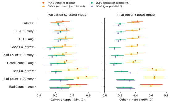
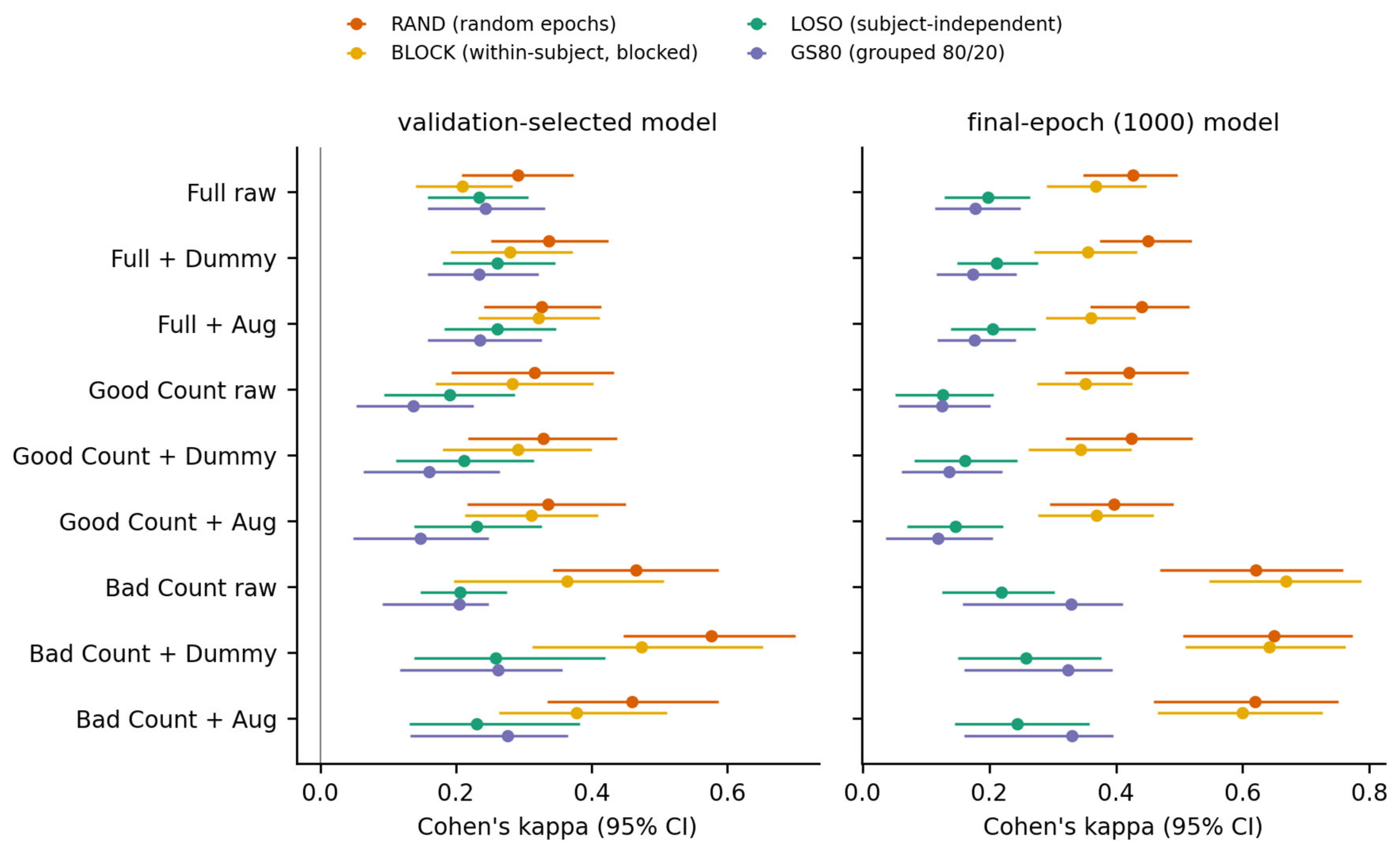
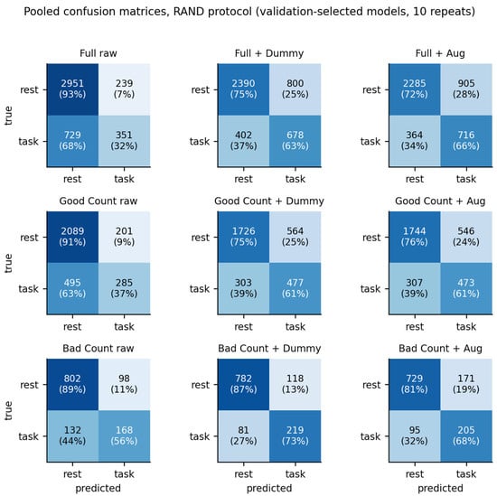
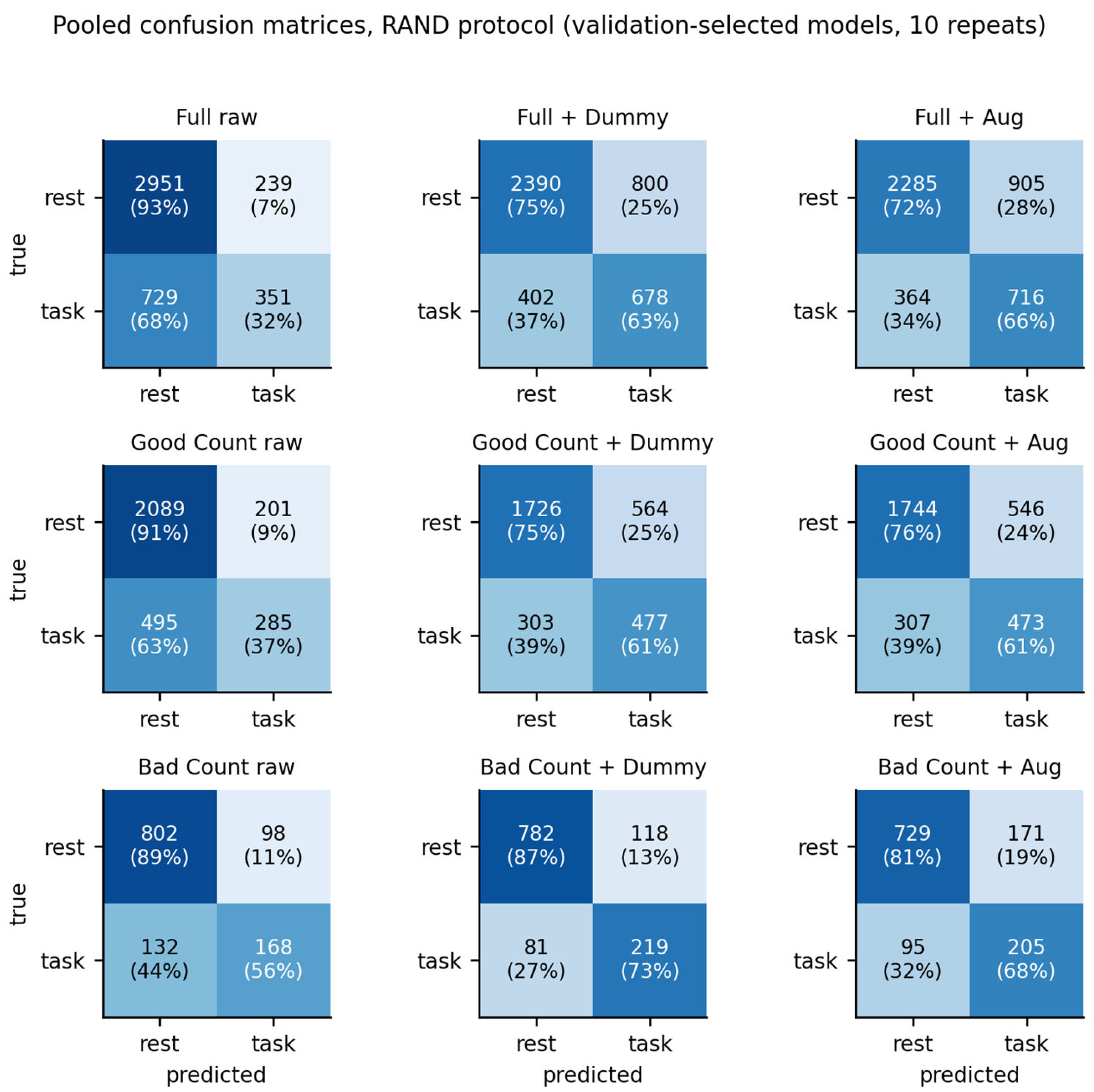
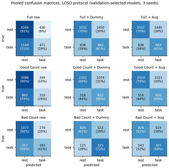
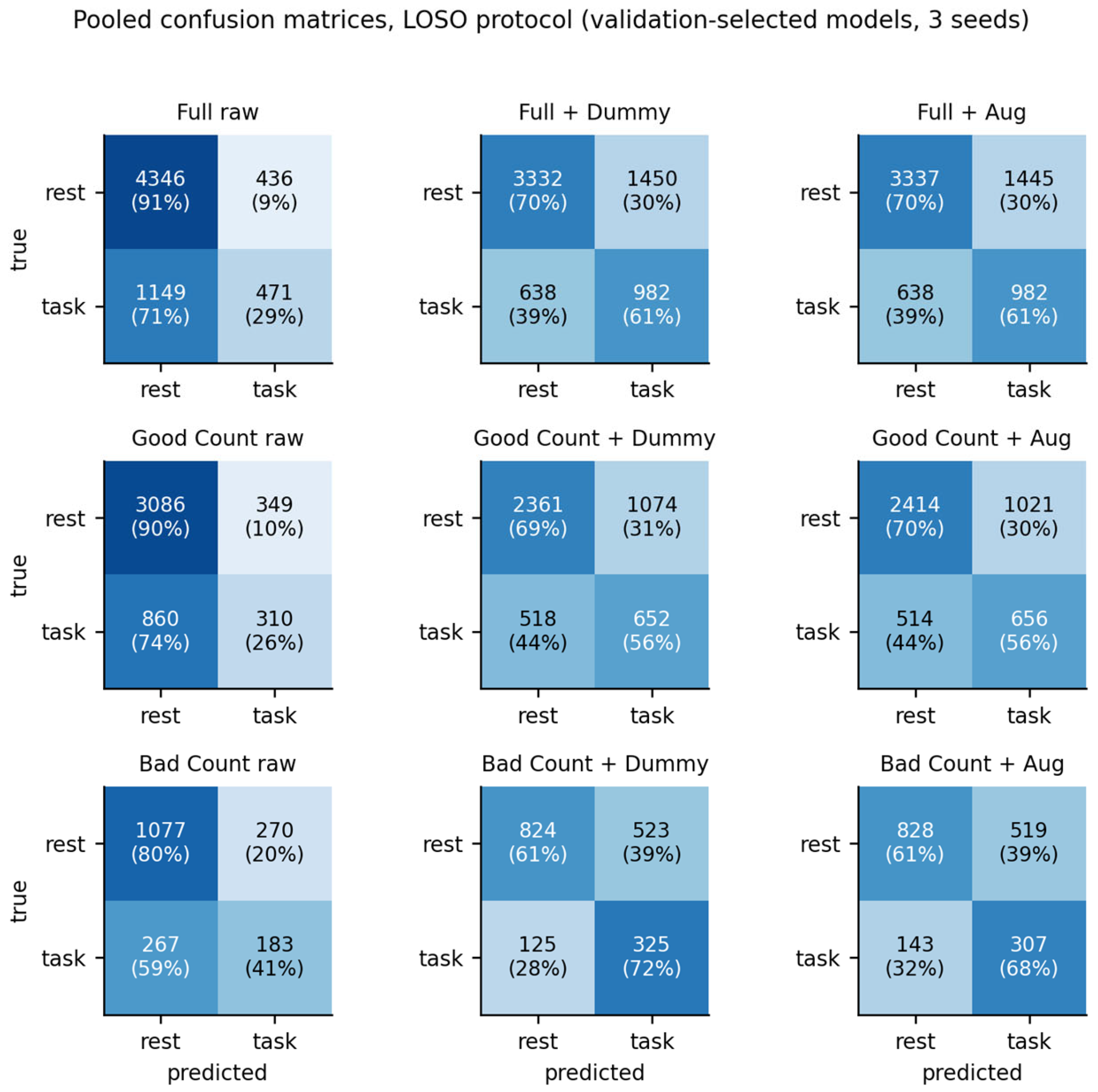
Table 1 reports Cohen’s kappa for the 36 conditions (3 pools × 3 training-set modes × 4 protocols), for the validation-selected model with its 95% subject-cluster bootstrap interval and for the final-epoch model. Table 2 gives the complete set of metrics for the two protocols that bracket the question (RAND and LOSO). Figure 2 shows the kappa values with their intervals and Figure 3 and Figure 4 the pooled confusion matrices.
Table 1.
Cohen’s kappa by protocol and training-set mode. “Sel.” = validation-selected model, mean [95% subject-cluster bootstrap CI]; “Fin.” = final-epoch (1000) model. RAND and GS80: mean over 10 and 20 repetitions; BLOCK: pooled five-fold out-of-fold predictions; LOSO: mean over 3 seeds.
Table 2.
Full metric set for the validation-selected models under the subject-dependent random epoch split (RAND) and the subject-independent leave-one-subject-out protocol (LOSO). Prev. = task prevalence of the test sets; Sens. = recall of task; Spec. = recall of rest; mean [95% CI] for balanced accuracy and ROC-AUC. N test = test items per run (BLOCK and LOSO: pooled over folds).
Figure 2.
Cohen’s kappa (mean and 95% subject-cluster bootstrap interval) for the 36 conditions, for the validation-selected (left) and final-epoch (right) models.
Figure 3.
Pooled confusion matrices of the validation-selected models, random epoch split (RAND). Counts and row percentages.
Figure 4.
Pooled confusion matrices of the validation-selected models, leave-one-subject-out (LOSO). Counts and row percentages.
With balancing confined to the training partitions, the subject-dependent random epoch split yields kappa 0.29–0.58 (balanced accuracy 0.63–0.80, ROC-AUC 0.75–0.88) for the validation-selected models and kappa 0.40–0.65 for the final-epoch models. These values are far below the 88–99% accuracies (kappa 0.66–0.98) of the published windowed-split literature. Under the subject-independent LOSO protocol, kappa is 0.19–0.26 (balanced accuracy 0.58–0.67, ROC-AUC 0.66–0.71) for the validation-selected and 0.13–0.26 for the final-epoch models. The repeated grouped 80/20 protocol gives kappa 0.14–0.28 (validated) with a split-to-split standard deviation of up to 0.15, about 6 times the seed-to-seed spread of LOSO on the same pool. In no subject-independent condition does the kappa interval include 0, so a genuine but modest subject-independent signal exists in these simple statistics.
3.2. Per-Class Performance and Confusion Matrices
Table 2 reports sensitivity, specificity and F1 of the task class; Figure 3 and Figure 4 show the pooled confusion matrices of the validation-selected models. The task class carries the errors in every model. Under LOSO, task sensitivity is 0.26–0.72 and specificity 0.61–0.91; raw training sets favour the majority class (sensitivity 0.26–0.41), whereas Dummy and Aug training raises sensitivity to 0.56–0.72 at the cost of specificity (0.61–0.70). Under RAND, task sensitivity is 0.33–0.73 and specificity 0.72–0.93.
3.3. Effect of the Training-Set Mode
Raw versus balanced. Balancing the training set raises balanced accuracy at the cost of accuracy, because it shifts the decision threshold towards the minority class; kappa changes much less. Under LOSO the kappa gain from Dummy or Aug relative to raw is at most 0.05, and in several pools the intervals overlap. Balancing is therefore useful mainly for the balance between the two error types, not for discrimination (ROC-AUC under LOSO: 0.66–0.71 for all nine modes).
Dummy versus augmented. Differences between the two balancing strategies are small and mostly not distinguishable from 0: the Dummy minus Aug difference in kappa under LOSO is −0.02 to 0.03 (validated models) and 0.01 (final-epoch models). The one exception is the Bad Count pool under the random epoch split, where Dummy exceeds Aug by 0.12 (validated). This is tested formally in Section 4.2.
Good versus bad counters. Bad Count models, trained on 10 subjects, show the largest subject-dependent advantage (RAND kappa 0.46–0.58 versus LOSO 0.21–0.26), consistent with memorization of a few individuals; Good Count and Full models are steadier (RAND minus LOSO kappa 0.06–0.13).
Subject-dependent excess. The paired bootstrap difference κ(RAND) − κ(LOSO) for the validation-selected models is 0.06–0.08 (Full), 0.10–0.13 (Good Count) and 0.23–0.32 (Bad Count); every interval excludes 0 (lower limits 0.02 to 0.16). The chronologically blocked within-subject protocol lies in between (BLOCK minus LOSO: −0.02 to 0.22), so part of the subject-dependent advantage persists when neighbouring epochs are removed from training.
3.4. Control: Balancing Before Splitting (Original Order of Operations)
The original design, from the existing literature, placed duplicated or augmented samples on both sides of the epoch-level split and used balanced or augmented test sets, so that the very high scores could not be attributed cleanly to subject identity. We reproduced this order of operations as an explicit control (PRE): the pool is balanced first (Dummy duplicates or augmented copies), then split at random 80/20 (10 repetitions), so that the test partition has prevalence 0.5 and consists partly of copies. For every test item we recorded whether its source epoch, or a copy of it, is in the training or validation partition. In Table 3 there are presented the results for control condition, where “Twin in train” means share of test items whose source epoch (or an identical or augmented copy of it) is in the training/validation data, and κ(RAND) means same pool and mode with balancing inside the training partition only (Table 1).
Table 3.
Control condition PRE (balance first, then random split; original order of operations), mean ± standard deviation over 10 repetitions, validation-selected models.
The PRE control gives accuracy 0.885–0.940, kappa 0.77–0.88 and ROC-AUC 0.945–0.981, at the level of the windowed-split literature, whereas the same pools and the same network under a correct random epoch split give kappa 0.33–0.58 and under LOSO 0.21–0.26. Between 45% and 47% of the PRE test items have a copy of their own source epoch in the training or validation data, and the accuracy on these items (0.95–0.99) is clearly higher than on the others (0.83–0.90). So, most of this inflation is conventional duplicate and augmented-copy contamination (together with the balanced test set), and only a smaller part is attributable to subject dependence, which is quantified in Section 3.3.
3.5. Early Stopping Versus Continued Training
Table 4 compares the final-epoch and the validation-selected models. The validation criterion selects very early epochs (median selected epoch 1–9 over all conditions), so the validation-selected network is a lightly trained one.
Table 4.
Effect of continued training: κ of the validation-selected (Sel.) and final-epoch (Fin.) models and their paired difference Δ = Fin. − Sel. [95% bootstrap CI].
Continued training raises kappa in the subject-dependent protocols (RAND: Δ = 0.06–0.16; BLOCK: 0.04–0.31) and lowers it or leaves it unchanged in the subject-independent protocol (LOSO: −0.08 to 0.01). Reporting only the final-epoch model would slightly understate the subject-independent performance and, more importantly, overstate the subject-dependent performance relative to the validation-selected one. This asymmetry is itself informative: additional epochs after the validation optimum improve test results only when the test data share subjects (and, for RAND, neighbouring time points) with the training data, which is the signature of memorization of recording-specific patterns.
3.6. Subject-Level Analysis
Because epochs are clustered within subjects, Table 5 summarises the performance at the level of the individual subject for the validation-selected models. Median per-subject balanced accuracy; share of subjects above 0.5 and one-sided Wilcoxon p; share of subjects whose mean predicted task probability is higher on the task than on the rest recording and one-sided sign-test p.
Table 5.
Per-subject analysis of the validation-selected models.
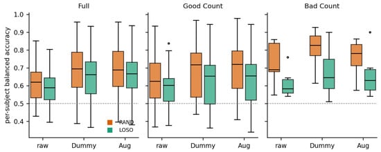
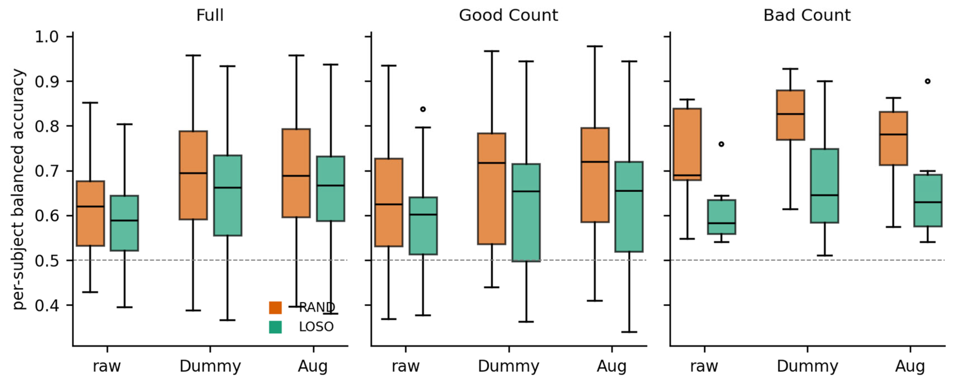
Under LOSO, the median per-subject balanced accuracy (Figure 5) is 0.58–0.67, 73% to 100% of the subjects are above 0.5 (all Wilcoxon p ≤ 0.001), and in 77% to 100% of the subjects the mean predicted task probability is higher on the task than on the rest recording (all sign-test p ≤ 0.005). The subject-independent signal is therefore a statistically reliable, group-level effect, but individual subjects range from clearly informative to at or below chance, and the small number of subjects (10, 26, 36) limits the precision of every estimate.
Figure 5.
Distribution of per-subject balanced accuracy for the validation-selected models (RAND and LOSO).
3.7. Quantifying Information Content: Mutual Information and Entropy Diagnostics
Table 6 reports, for the RAND and LOSO protocols, the label entropy H(Y), mutual information I(Y;Ŷ), the normalized transfer I/H(Y), the residual entropy H(Y|Ŷ), normalized mutual information (NMI), adjusted mutual information (AMI) and confusion entropy (CEN) computed from the pooled confusion matrices of the validation-selected models (Section 2.8).
Table 6.
Label entropy and mutual information diagnostics from pooled confusion matrices (bits), validation-selected models. H(Y) is identical to its normalized value H(Y)/log2|| because || = 2.
Under the reported design the information transferred is small in absolute terms. Subject-independent models resolve 3% to 8% of the label entropy (I = 0.027–0.062 bits per epoch), subject-dependent random-split models 8% to 28% (I = 0.062–0.226 bits). Mutual information still has a non-negative lower bound and is blind to the sign of the association, so it should be read together with kappa, ROC-AUC and CEN; with natural ratio test sets the confusion entropy tends to be higher (more diffuse errors) under LOSO (0.63–0.81) than under RAND (0.56–0.75).
3.8. Cross-Entropy Training-Loss Dynamics
Table 7 reports, for the RAND and LOSO protocols, the training and test cross-entropy dynamics (condition-mean curves), the oracle epoch of best test accuracy and the epoch picked by validation.
Table 7.
Accuracy and cross-entropy dynamics (condition-mean curves over all runs; nats). Best acc. @ep = best mean test accuracy and its epoch (oracle, uses test data); Min test CE @ep = minimum mean test cross-entropy and epoch; Gap@best = test minus train CE at that epoch; CE rise = final minus minimum test CE; Val. ep = median epoch selected by validation.
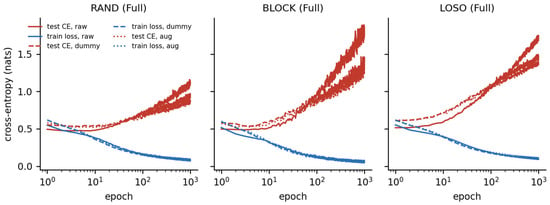
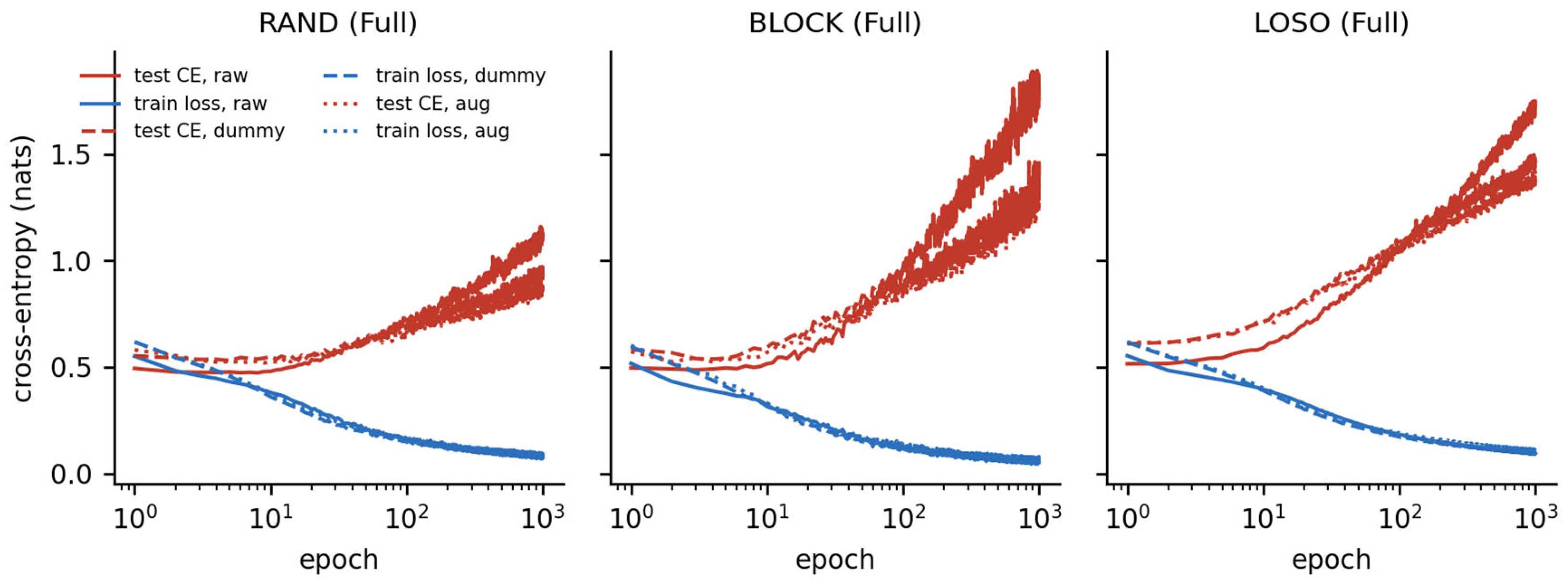
In every condition the test cross-entropy reaches its minimum within the first 9 epochs (LOSO: epoch 1–2; RAND: epoch 3–9) and then rises by 0.34–2.84 nats while the training accuracy approaches 1. The generalization gap at the best epoch is +0.02 to +0.20 nats under RAND and −0.04 to +0.09 under LOSO, i.e., the two ranges overlap. The epoch of best test accuracy is very early under LOSO (epoch 1–2 for the raw pools) but late under the subject-dependent random split (epoch 364–736 for the raw pools) (Figure 6), in line with Section 3.5.
Figure 6.
Mean training loss and test cross-entropy versus epoch (logarithmic axis) for the Full pool, protocols RAND, BLOCK and LOSO, and the three training-set modes.
3.9. Model Weight and Spectral Entropy
Spectral measures of the final-epoch networks are narrowly distributed across all 36 conditions: layer-1 effective rank 37.4–43.9 of 57 (nER 0.66–0.77), layer-2 effective rank 21.5–23.7 of 32 (nER 0.67–0.74), and batch-normalization scale entropy 0.991–0.999, so no hidden unit is switched off (Table 8). The validation-selected networks, which are lightly trained, have a higher normalized effective rank (0.81–0.87) than the final-epoch networks (0.68–0.75); the profile is otherwise invariant to the protocol and to the training-set mode. Spectral entropy thus characterizes the training stage, not the evaluation protocol.
Table 8.
Weight-matrix spectral entropy and effective rank (mean over all networks of a condition; range over the nine pool/mode conditions in brackets), by protocol and model (final-epoch or validation-selected).
3.10. SHAP Explanation Entropy
SHAP attributions are diffuse: feature evenness 0.86–0.93, channel evenness 0.93–0.97, and the largest single feature carries 15% of the total attribution at most (LOSO models are somewhat more concentrated than RAND models for the Full pool: top-1 share 0.14 versus 0.08) (Table 9). Averaged over the LOSO models, the standard deviation accounts for 56%, the skewness for 26% and the mean for 18% of the attribution; the highest-ranked channels are frontal (Fp1, F8, Fp2) followed by Cz and T3. A prominent role of frontal leads is plausible for a cognitive-load contrast but may also reflect residual ocular or frontal-muscle activity after ICA cleaning, which we did not test. The Jensen–Shannon distance between the feature-importance distributions of RAND and LOSO models of the same condition is 0.12–0.22 bits1/2 and between LOSO conditions 0.09–0.24, i.e., modest.
Table 9.
SHAP explanation entropy of validation-selected models (57 features = 19 channels × 3 statistics; mean of six networks).
3.11. Feature-Set Ablation: Redundant RMS, Skewness, and Non-EEG Channels
Table 10 presents the ablation of the feature set, with the validation-selected models, RAND and LOSO; κ and ROC-AUC, where msk19 = µ, σ, γ, on 19 EEG channels (main analysis); msr19 = µ, σ, RMS on the 19 EEG channels; msr21 = µ, σ, RMS on all 21 channels (original configuration, including A2-A1 and ECG).
Table 10.
Ablation of the feature set.
Replacing skewness by the redundant RMS leaves the subject-independent result essentially unchanged (LOSO kappa 0.17–0.26 versus 0.19–0.26) but raises the subject-dependent result substantially (RAND kappa 0.44–0.69 versus 0.29–0.58; ROC-AUC 0.83–0.94 versus 0.75–0.88). Including the A2-A1 and ECG channels increases it further (RAND kappa 0.46–0.75) while slightly lowering the subject-independent result (LOSO kappa 0.16–0.22). The subject-dependent gain with RMS is consistent with amplitude features acting as recording-specific fingerprints: the unscaled µ/σ/RMS statistics encode electrode and recording conditions that are stable within a subject and recording, whereas the γ is scale-free. Consequently, the size of the subject-dependent inflation depends on the feature set, and the µ, σ, RMS feature choice, together with the non-EEG channels, was among the configurations most favourable to subject-dependent inflation.
3.12. Comparison with the Published EEGMAT Literature
Table 11 places the results of this study alongside prior EEGMAT classification studies, distinguishing studies using a windowed/random-split protocol (comparable to our subject-dependent conditions) from the rarer subject-independent (LOSO) studies.
Table 11.
Comparison with published EEGMAT classification studies.
Most published EEGMAT work segments each recording into short (2–4 s) windows, pools windows across all 36 subjects, and splits at random. Our PRE control, which follows that order of operations, reproduces accuracies in the high 80s to low 90s with only three statistics per channel, but a correct random epoch split with the same features does not, and a subject-independent evaluation gives a balanced accuracy of 58–67% (ROC-AUC 0.66–0.71). The strongest subject-independent studies use substantially richer, spectrally and structurally derived features and report 97–98% [22,23].
4. Discussion
4.1. Which Validation Design Answers Which Question
If the aim is to characterize how the brain activity of a given person changes between rest and task, subject-dependent evaluation is appropriate, provided that dependent data are separated: neighbouring epochs of one recording are strongly autocorrelated, and in EEGMAT the class label is confounded with the recording (one rest and one task recording per subject), so a random epoch split rewards recognition of the recording rather than of the state. The chronologically blocked BLOCK protocol is the minimal safeguard, and it yields lower kappa than RAND for several conditions. If the aim is a detector for new users, subject-independent evaluation (LOSO) is required.
Quantitatively, the subject-dependent excess is real but moderate when the pipeline is clean: the paired difference of kappa between RAND and LOSO is 0.06–0.32 (all intervals exclude 0), and continued training helps only the subject-dependent protocols (Section 3.5). The much larger inflation of the kappa up to 0.95 came mainly from the order of operations (Section 3.4) and, to a degree that depends on the features, from amplitude statistics that act as recording fingerprints (Section 3.11).
Subject-identity leakage or inter-individual variability. The difference between the subject-dependent and the subject-independent results does not by itself establish subject identity as the underlying mechanism. EEG amplitude, oscillatory characteristics and task-related responses differ substantially between individuals, so a model trained on some participants is expected to perform worse on unseen participants even when no identity information is exploited; the lower LOSO performance is therefore at least partly the ordinary cross-subject generalization problem. What the present experiments show is more limited. The subject-dependent advantage is statistically reliable but moderate. It is smaller for validation-selected models than for final-epoch models, and continued training improves the results only when subjects are shared between training and test data (Section 3.5), which is the pattern expected from memorization of subject-specific or recording-specific patterns. It is larger with unscaled amplitude features and the non-EEG channels and smaller with a scale-free feature (Section 3.11). These observations are consistent with identity-related information being used, but each has alternative explanations: recording-specific regularities such as session drift or electrode impedance, the confounding of class with recording (Section 2.2), and the simple fact that a model that has seen a person’s own distribution fits it better than one that has not. A direct test would require, for example, predicting subject identity from the same features, subject-wise normalization of the features, or a comparison with a task-unrelated label; none of these was performed. We therefore describe the effect as a subject-dependent advantage and not as proven subject-identity leakage.
Insight beyond the known difficulty of cross-subject EEG generalization. That cross-subject generalization is difficult is well established [10]. For this widely used dataset the study adds a quantification showing that most of the very high published-style scores are explained by duplicate or augmented-copy contamination and not by neurophysiological differences between participants or by subject identity; the size of the remaining subject-dependent advantage, with confidence intervals and its dependence on the features and on the stopping rule; and a set of checks (counting test items with a copy in the training data, a chronologically blocked protocol, the comparison of validation-selected with final-epoch models) that can be applied to other pipelines.
4.2. Balancing Strategy and Protocol: Is There an Interaction?
For the Full and Good Count pools the difference between Dummy and Aug is within about ±0.04 kappa under every protocol (the one interval that excludes 0 is Full under BLOCK, −0.04, where Aug is slightly better) and the RAND-minus-LOSO difference of differences includes 0 (Table 12). Only for the Bad Count pool and the validation-selected models is the difference of differences different from 0 (0.09, 95% CI 0.04 to 0.14), and it disappears for the final-epoch models (0.02, CI −0.01 to 0.05). Given the number of comparisons and the small number of subjects, we regard this as at best a weak, pool-specific effect, not as a diagnostic. The original gap (Good Count kappa 0.916 versus 0.743) was produced by duplicates that fall on both sides of the split (Section 3.4), not by the balancing strategy as such.
Table 12.
Dummy minus Aug difference in κ per protocol and difference of differences (RAND minus LOSO), paired subject-cluster bootstrap, validation-selected and final-epoch models. Estimate [95% CI], two-sided p.
4.3. Diagnostics and Benchmarking Against the Literature
Mutual information is non-negative by construction and cannot distinguish a systematically inverted classifier from an uninformative one, so it must be read together with kappa, ROC-AUC and confusion entropy. No condition in the present experiments has a negative kappa, so this sign-blindness is a caution rather than an observed problem.
The cross-entropy curves show that every model overfits rapidly in all protocols, which is why a validation-based stopping rule changes the results (Section 3.5). The generalization gap at the best epoch does not separate subject-dependent from subject-independent protocols, because the two ranges overlap (Section 3.8), so it is not suitable as an indicator of the evaluation design. The curves remain useful for choosing the stopping epoch. Likewise, the spectral profile of the weights and the diffuseness of SHAP explanations vary little across protocols and training-set modes, whereas the weight spectra depend on the training stage (validation-selected versus final-epoch networks). Capacity use and explanation entropy are therefore properties of the architecture and the training budget; they do not signal whether an evaluation protocol is subject-dependent. This is consistent with the commitment articulated in Section 1.5, that structural properties of a network and the trustworthiness of its reported performance are distinct questions.
Our subject-independent balanced accuracy (58–67%) is far below the 97–98% reported by leave-one-subject-out studies with richer features [22,23], and our subject-dependent results under a correct split are also well below the windowed-split literature [17,18,19,20,21]. The difference between the balance-then-split control and the correct random epoch split shows that the order of operations can by itself produce scores in the high 80s to low 90s. This warrants caution when interpreting published windowed-split numbers, without implying that those studies share the same error; the sources of their performance would have to be checked individually. Our minimal feature set is a limiting factor, and the weak subject-independent signal should not be read as an upper bound for EEG-based cognitive-workload detection. Because only the mean, standard deviation and skewness of the amplitude distribution were used, the limited subject-independent performance may reflect this feature representation and not an inherent limit of cross-subject EEG generalization.
4.4. Limitations
The modest number of subjects (36 in total, with only 10 in the Bad Count group) limits the precision of every estimate. Uncertainty is quantified by repeated splits and subject-cluster bootstrap intervals, but the intervals reflect sampling of these 36 subjects only; the Bad Count pool in particular has wide intervals and the grouped 80/20 protocol has only two test subjects per split.
In this paper “subject-independent” and “leakage-free” are defined with respect to the available subject pool: no test subject contributes data, original or augmented, to training. They do not imply generalization to an independent population. Augmented epochs are derived from the same 36 subjects; hence, they are not independent data, and even subject-independent evaluation here measures generalization across a fixed pool of 36 subjects recorded in one laboratory.
The labels come from the recording (rest versus task), so a classifier may in principle exploit any systematic difference between the two recording sessions (duration, drift, adaptation) in addition to mental workload. The rest recordings are three times longer than the task recordings, and no balanced duration-matched analysis was performed.
Augmentation hyperparameters (5% noise fraction, 0.9–1.1 scale range, 5% shift fraction) were set at their code-default values and not tuned, and the shift has no effect on the order-invariant statistics used here. Validation-based model selection uses a single 15% validation partition per split.
The feature set is restricted to simple time-domain per-channel statistics; frequency-domain (band power), connectivity, and entropy-based EEG features were deliberately excluded and remain a natural extension for narrowing the gap to the richer-feature literature (Section 3.12 and Section 4.3).
Only one classifier (an MLP) and one family of features were examined. The mean, standard deviation and skewness of the amplitude distribution do not target established neurophysiological correlates of mental arithmetic, such as the increase of frontal theta activity and the modulation of alpha activity with cognitive load [48], and they may mainly capture individual or recording-specific amplitude characteristics instead of task-related neural responses. The modest subject-independent performance therefore cannot be taken as evidence of an inherent limit of cross-subject EEG generalization, and our conclusions about the subject-dependent advantage are restricted to this classifier and this feature family; other classifiers and spectral features (band power, frontal-midline theta, alpha) may show a different gap. The SHAP results, with frontal channels ranked highest, are compatible with a frontal contribution but cannot be interpreted as theta activity because no spectral features were used.
The sizes of the Good Count and Bad Count pools follow the subject-information file (26 and 10 subjects), whereas the dataset description lists 24 and 12 (Section 2.1). Under the alternative grouping each of these pools would change by two subjects, so the pool-specific results, especially those of the 10-subject Bad Count pool, should be read with this uncertainty; the Full pool results are unaffected.
5. Conclusions
Using four evaluation protocols, three subject pools and three training-set modes (more than 1000 trained MLPs), we re-examined how much of the very high EEGMAT rest-versus-mental-arithmetic accuracy survives a design in which balancing and augmentation are confined to the training partitions, the test sets are untouched, models are selected on validation data and uncertainty is quantified by repeated splits and subject-cluster bootstrap. With a correct random epoch split, three amplitude-distribution statistics per channel give kappa 0.29–0.58 (validation-selected models); a control that reproduces the original order of operations (balance, then split) gives kappa 0.77–0.88 and has 45–47% of its test items duplicated in training, so most of this inflation was conventional duplicate contamination and not subject identity as such. Subject dependence adds a smaller, statistically reliable increment (paired kappa difference RAND minus LOSO 0.06–0.32), which increases when the features carry recording-specific amplitude information (RMS, ECG and A2-A1 channels) and which shows up as a gain from continued training that is absent in subject-independent testing. This increment is consistent with, but does not prove, subject-identity leakage: normal inter-individual variability and the restricted classifier and feature set cannot be separated from it here. Leave-one-subject-out evaluation yields kappa 0.19–0.26, balanced accuracy 58–67% and ROC-AUC 0.66–0.71: a reliable group-level but modest subject-independent signal, with substantial between-subject variability.
Neither subject-dependent nor subject-independent evaluation is wrong in itself; each answers a different question, and published scores should be interpreted accordingly. “Leakage-free” here means free of train/test contamination with respect to the available pool of 36 subjects, not generalizable to the population. Mutual information must still be read together with kappa, ROC-AUC and confusion entropy, and weight spectral entropy and SHAP entropy are properties of the training stage and architecture rather than of the evaluation protocol. To our knowledge, this is the first study on the EEGMAT dataset to quantify these effects.
Author Contributions
Conceptualization, R.S., M.L. and A.I.; methodology, A.I.; software, R.S. and M.L.; validation, M.L., and A.I.; formal analysis, M.L.; investigation, R.S.; resources, R.S.; data curation, R.S.; writing—original draft preparation, R.S.; writing—review and editing, M.L. and A.I.; visualization, M.L. and A.I.; supervision, M.L.; project administration, A.I.; funding acquisition, R.S. All authors have read and agreed to the published version of the manuscript.
Funding
This research received no external funding.
Institutional Review Board Statement
Ethical review and approval were waived for this study due to the use of a public dataset.
Data Availability Statement
The source code developed for this research is available at https://github.com/monicaleba/entropy_EEGMAT (accessed on 12 September 2026).
Acknowledgments
The author acknowledges the University of Petroșani for institutional support during the preparation of this work. The author also acknowledges the use of large language model assistants, i.e., Anthropic Claude Opus 4.8 model, for editorial review and code verification during manuscript preparation; all conceptual contributions, experimental design, and analytical conclusions are the authors’ own. The authors have reviewed and edited the output of GenAI and take full responsibility for the content of this publication.
Conflicts of Interest
The authors declare no conflicts of interest.
References
- Katmah, R.; Al-Shargie, F.; Tariq, U.; Babiloni, F.; Al-Mughairbi, F.; Al-Nashash, H. A review on mental stress assessment methods using EEG signals. Sensors 2021, 21, 5043. [Google Scholar] [CrossRef] [Scilit]
- Dong, Y.; Xu, L.; Zheng, J.; Wu, D.; Li, H.; Shao, Y.; Shi, G.; Fu, W. A hybrid EEG-based stress state classification model using multi-domain transfer entropy and PCANet. Brain Sci. 2024, 14, 595. [Google Scholar] [CrossRef] [Scilit]
- Yao, L.; Wang, M.; Lu, Y.; Li, H.; Zhang, X. EEG-based emotion recognition by exploiting fused network entropy measures of complex networks across subjects. Entropy 2021, 23, 984. [Google Scholar] [CrossRef] [Scilit]
- Lo Giudice, M.; Varone, G.; Ieracitano, C.; Mammone, N.; Tripodi, G.G.; Ferlazzo, E.; Gasparini, S.; Aguglia, U.; Morabito, F.C. Permutation entropy-based interpretability of convolutional neural network models for interictal EEG discrimination of subjects with epileptic seizures vs. psychogenic non-epileptic seizures. Entropy 2022, 24, 102. [Google Scholar] [CrossRef] [Scilit]
- Kaufman, S.; Rosset, S.; Perlich, C.; Stitelman, O. Leakage in data mining: Formulation, detection, and avoidance. ACM Trans. Knowl. Discov. Data 2012, 6, 15. [Google Scholar]
- Kapoor, S.; Narayanan, A. Leakage and the reproducibility crisis in machine-learning-based science. Patterns 2023, 4, 100804. [Google Scholar] [CrossRef] [Scilit]
- Roberts, D.R.; Bahn, V.; Ciuti, S.; Boyce, M.S.; Elith, J.; Guillera-Arroita, G.; Hauenstein, S.; Lahoz-Monfort, J.J.; Schröder, B.; Thuiller, W.; et al. Cross-validation strategies for data with temporal, spatial, hierarchical, or phylogenetic structure. Ecography 2017, 40, 913–929. [Google Scholar] [CrossRef] [Scilit]
- Varoquaux, G.; Raamana, P.R.; Engemann, D.A.; Hoyos-Idrobo, A.; Schwartz, Y.; Thirion, B. Assessing and tuning brain decoders: Cross-validation, caveats, and guidelines. NeuroImage 2017, 145, 166–179. [Google Scholar] [CrossRef] [Scilit]
- Saeb, S.; Lonini, L.; Jayaraman, A.; Mohr, D.C.; Kording, K.P. The need to approximate the use-case in clinical machine learning. GigaScience 2017, 6, gix019. [Google Scholar] [CrossRef] [Scilit]
- Lotte, F.; Bougrain, L.; Cichocki, A.; Clerc, M.; Congedo, M.; Rakotomamonjy, A.; Yger, F. A review of classification algorithms for EEG-based brain-computer interfaces: A 10 year update. J. Neural Eng. 2018, 15, 031005. [Google Scholar] [CrossRef] [Scilit]
- Brookshire, G.; Kasper, J.; Blauch, N.M.; Wu, Y.C.; Glatt, R.; Merrill, D.A.; Gerrol, S.; Yoder, K.J.; Quirk, C.; Lucero, C. Data leakage in deep learning studies of translational EEG. Front. Neurosci. 2024, 18, 1373515. [Google Scholar] [CrossRef] [Scilit]
- Joloudari, J.H.; Marefat, A.; Nematollahi, M.A.; Oyelere, S.S.; Hussain, S. Effective class-imbalance learning based on SMOTE and convolutional neural networks. Appl. Sci. 2023, 13, 4006. [Google Scholar] [CrossRef] [Scilit]
- Chen, R.; Ma, X.; Li, X.; Sui, L.; Maeda, T.; Chen, Q.; Cao, J. EEG signal classification with data augmentation for epileptic focus localization and deep sleep detection. Sensors 2026, 26, 474. [Google Scholar] [CrossRef] [Scilit]
- Martins, F.M.; González Suárez, V.M.; Villar Flecha, J.R.; García López, B. Data augmentation effects on highly imbalanced EEG datasets for automatic detection of photoparoxysmal responses. Sensors 2023, 23, 2312. [Google Scholar] [CrossRef] [Scilit]
- Zyma, I.; Tukaev, S.; Seleznov, I.; Kiyono, K.; Popov, A.; Chernykh, M.; Shpenkov, O. Electroencephalograms during mental arithmetic task performance. Data 2019, 4, 14. [Google Scholar] [CrossRef] [Scilit]
- Salankar, N.; Mishra, P.; Garg, L. Stress classification by multimodal physiological signals using variational mode decomposition and machine learning. J. Healthc. Eng. 2021, 2021, 2146369. [Google Scholar] [CrossRef] [Scilit]
- Goenka, U.; Patil, P.; Gosalia, K.; Jagetia, A. Classification of electroencephalograms during mathematical calculations using deep learning. arXiv 2022, arXiv:2209.00627. [Google Scholar]
- Ganguly, B.; Chatterjee, A.; Mehdi, W.; Sharma, S.; Garai, S. EEG based mental arithmetic task classification using a stacked long short term memory network for brain-computer interfacing. In Proceedings of the IEEE VLSI Device Circuit and System (VLSI DCS), Kolkata, India, 18–19 July 2020; pp. 89–94. [Google Scholar]
- Fatimah, B.; Javali, A.; Ansar, H.; Harshitha, B.T.; Kumar, H. Mental arithmetic task classification using Fourier decomposition method. In Proceedings of the International Conference on Communication and Signal Processing (ICCSP); IEEE: Piscataway, NJ, USA, 2020; pp. 46–50. [Google Scholar]
- Fatimah, B.; Pramanick, D.; Shivashankaran, P. Automatic detection of mental arithmetic task and its difficulty level using EEG signals. In Proceedings of the 11th International Conference on Computing, Communication and Networking Technologies (ICCCNT); IEEE: Piscataway, NJ, USA, 2020; pp. 1–6. [Google Scholar]
- Varshney, A.; Ghosh, S.K.; Padhy, S.; Tripathy, R.K.; Acharya, U.R. Automated classification of mental arithmetic tasks using recurrent neural network and entropy features obtained from multi-channel EEG signals. Electronics 2021, 10, 1079. [Google Scholar] [CrossRef] [Scilit]
- Aslam, M. Electroencephalograph (EEG) based classification of mental arithmetic using explainable machine learning. Biocybern. Biomed. Eng. 2025, 45, 154–169. [Google Scholar] [CrossRef] [Scilit]
- Baygin, M.; Barua, P.D.; Dogan, S.; Tuncer, T.; Palmer, E.E.; Tan, R.-S.; Acharya, U.R. Automated mental arithmetic performance detection using quantum pattern- and triangle pooling techniques with EEG signals. Expert Syst. Appl. 2023, 227, 120306. [Google Scholar] [CrossRef] [Scilit]
- Lundberg, S.M.; Lee, S.-I. A unified approach to interpreting model predictions. Adv. Neural Inf. Process. Syst. 2017, 30, 4765–4774. [Google Scholar]
- Bhatt, U.; Weller, A.; Moura, J.M.F. Evaluating and aggregating feature-based model explanations. In Proceedings of the 29th International Joint Conference on Artificial Intelligence (IJCAI-20), Yokohama, Japan, 7–15 January 2021; pp. 3016–3022. [Google Scholar]
- Hettikankanamage, N.; Shafiabady, N.; Chatteur, F.; Wu, R.M.X.; Ud Din, F.; Zhou, J. eXplainable Artificial Intelligence (XAI): A systematic review for unveiling the black box models and their relevance to biomedical imaging and sensing. Sensors 2025, 25, 6649. [Google Scholar] [CrossRef] [Scilit]
- Ionica, A.; Leba, M. From house of quality to neural architecture: Quality-informed neural networks for interpretable classification, with an EU AI Act compliance application. Systems 2026, 14, 647. [Google Scholar] [CrossRef] [Scilit]
- Triohin, V.; Leba, M.; Ionica, A.C. From convolution to spikes for mental health: A CNN-to-SNN approach using the DAIC-WOZ dataset. Appl. Sci. 2025, 15, 9032. [Google Scholar] [CrossRef] [Scilit]
- Wei, J.-M.; Yuan, X.-J.; Hu, Q.-H.; Wang, S.-Q. A novel measure for evaluating classifiers. Expert Syst. Appl. 2010, 37, 3799–3809. [Google Scholar] [CrossRef] [Scilit]
- Roy, O.; Vetterli, M. The effective rank: A measure of effective dimensionality. In Proceedings of the 15th European Signal Processing Conference (EUSIPCO), Poznań, Poland, 3–7 September 2007; pp. 606–610. [Google Scholar]
- Hill, M.O. Diversity and evenness: A unifying notation and its consequences. Ecology 1973, 54, 427–432. [Google Scholar] [CrossRef] [Scilit]
- Pielou, E.C. The measurement of diversity in different types of biological collections. J. Theor. Biol. 1966, 13, 131–144. [Google Scholar] [CrossRef] [Scilit]
- Joanes, D.N.; Gill, C.A. Comparing measures of sample skewness and kurtosis. J. R. Stat. Soc. Ser. D 1998, 47, 183–189. [Google Scholar] [CrossRef] [Scilit]
- Prechelt, L. Early stopping-but when? In Neural Networks: Tricks of the Trade; Springer: Berlin, Germany, 1998; pp. 55–69. [Google Scholar] [CrossRef] [Scilit]
- Efron, B.; Tibshirani, R.J. An Introduction to the Bootstrap; Chapman & Hall: New York, NY, USA, 1994. [Google Scholar] [CrossRef] [Scilit]
- Cameron, A.C.; Gelbach, J.B.; Miller, D.L. Bootstrap-based improvements for inference with clustered errors. Rev. Econ. Stat. 2008, 90, 414–427. [Google Scholar] [CrossRef] [Scilit]
- Wilcoxon, F. Individual comparisons by ranking methods. Biom. Bull. 1945, 1, 80–83. [Google Scholar] [CrossRef] [Scilit]
- Theil, H. On the estimation of relationships involving qualitative variables. Am. J. Sociol. 1970, 76, 103–154. [Google Scholar] [CrossRef] [Scilit]
- Kvalseth, T.O. Entropy and correlation: Some comments. IEEE Trans. Syst. Man. Cybern. 1987, 17, 517–519. [Google Scholar] [CrossRef] [Scilit]
- Strehl, A.; Ghosh, J. Cluster ensembles—A knowledge reuse framework for combining multiple partitions. J. Mach. Learn. Res. 2002, 3, 583–617. [Google Scholar]
- Vinh, N.X.; Epps, J.; Bailey, J. Information theoretic measures for clusterings comparison: Variants, properties, normalization and correction for chance. J. Mach. Learn. Res. 2010, 11, 2837–2854. [Google Scholar]
- Jurman, G.; Riccadonna, S.; Furlanello, C. A comparison of MCC and CEN error measures in multi-class prediction. PLoS ONE 2012, 7, e41882. [Google Scholar] [CrossRef] [Scilit]
- Jost, L. Entropy and diversity. Oikos 2006, 113, 363–375. [Google Scholar] [CrossRef] [Scilit]
- Lin, J. Divergence measures based on the Shannon entropy. IEEE Trans. Inf. Theory 1991, 37, 145–151. [Google Scholar] [CrossRef] [Scilit]
- Cohen, J. A coefficient of agreement for nominal scales. Educ. Psychol. Meas. 1960, 20, 37–46. [Google Scholar] [CrossRef] [Scilit]
- Matthews, B.W. Comparison of the predicted and observed secondary structure of T4 phage lysozyme. Biochim. Biophys. Acta (BBA)-Protein Struct. 1975, 405, 442–451. [Google Scholar] [CrossRef] [Scilit]
- Fawcett, T. An introduction to ROC analysis. Pattern Recognit. Lett. 2006, 27, 861–874. [Google Scholar] [CrossRef] [Scilit]
- Klimesch, W. EEG alpha and theta oscillations reflect cognitive and memory performance: A review and analysis. Brain Res. Rev. 1999, 29, 169–195. [Google Scholar] [CrossRef] [Scilit]

Disclaimer/Publisher’s Note: The statements, opinions and data contained in all publications are solely those of the individual author(s) and contributor(s) and not of MDPI and/or the editor(s). MDPI and/or the editor(s) disclaim responsibility for any injury to people or property resulting from any ideas, methods, instructions or products referred to in the content. |
© 2026 by the authors. Licensee MDPI, Basel, Switzerland. This article is an open access article distributed under the terms and conditions of the Creative Commons Attribution (CC BY) license.