


Abstract
The edge-of-chaos hypothesis holds that recurrent systems near criticality maximize memory capacity and expressivity, motivating a natural proposal: replace the non-chaotic linear recurrence of state-space models with a learnable chaotic one. We test this with a gain-tunable chaotic cell whose expansion is set by one calibrated parameter, instrumented with a validated Lyapunov estimator, and measure delay-resolved memory capacity against the lagged mutual information each target demands. Trained end to end, the chaotic recurrence confers no benefit over a gated RNN or its own periodic-regime ablation; a gate dose–response identifies the learned gate as the suppressing mechanism. Frozen under the canonical reservoir-computing protocol, it decisively outperforms a matched linear reservoir, yet a regime-pure control () shows that this is not criticality: an ordered reservoir () matches or exceeds the critical one, and across six chaotic reservoir constructions, the ordered arm leads on 21 of 30 paired seeds. Criticality pays only where the target reaches far enough back, on Mackey–Glass and the Santa Fe laser, and delay-resolved measurement explains why: the ordered reservoir retains more at lags 1–3, the critical one retains two to three times more at lags 4–12, and across six targets, the critical margin tracks long-lag demand (Pearson ), changing sign. We propose a two-factor account: bounded nonlinearity under contraction is necessary, and among nonlinear reservoirs, task-matched memory decides.
1. Introduction
The past three years have reshaped sequence modeling. State-space models (SSMs) rooted in classical control theory—S4, S5, Mamba, Mamba-2, and, most recently, Mamba-3—have shown that linear recurrent systems with carefully designed state matrices can match or exceed Transformer [1] performance on long-range tasks at sub-quadratic cost in sequence length. Yet, the linear core of these models imposes a fundamental ceiling. A linear state-transition matrix encodes a fixed, stationary dynamical regime, and recent work makes this ceiling increasingly formal. Halloran et al. [2] derive bounds showing that the maximal Lyapunov exponent of Mamba and Mamba-2 blocks is non-positive; they present this as a stability property—small input perturbations do not lead to exponentially diverging outputs. However, the same property has a less benign reading for expressivity: a recurrence that is provably Lyapunov-stable cannot operate at or beyond criticality, and it is not clear that the ordered regime is where the richest computation lives. Complementary results show that Mamba lags S4D in expressiveness and stability on long-range tasks [3], that pure SSMs trail Transformers on tasks requiring strong copying or in-context learning [4], and that Mamba’s long-range memory decays strictly exponentially [5].
Against this backdrop, a natural and theoretically motivated hypothesis presents itself. Biological neural circuits are decidedly nonlinear, and a large literature argues that they operate near the edge of chaos—a critical regime in which information propagation, storage capacity, and computational expressivity are simultaneously maximized [6,7,8,9,10]. Parallel work in deep learning theory reports that trained networks near the edge of chaos exhibit maximal generalization, robustness to label noise, and rich rather than lazy learning dynamics [11,12,13]. If linear SSMs are limited precisely because they cannot leave the ordered regime, then endowing a sequence model with a learnable chaotic recurrence, regularized to sit near criticality, ought to confer the richer dynamics the linear core lacks. This is the hypothesis behind chaotic state-space models.
This paper tests that hypothesis directly, reporting that it fails on both of its terms and that what replaces it is neither chaos nor criticality but a matching condition between the reservoir and the task. We build a chaotic recurrent cell that is genuinely capable of chaos—showing that its instantaneous expansion rate is proportional to a single learnable gain and verifying with a validated estimator that it reaches positive Lyapunov exponents—and we train it end to end on synthetic sequence tasks alongside strong baselines. Trained this way, the chaotic recurrence confers no benefit. Through a causal ablation, a conditional Lyapunov analysis of the trained models, and a gate dose–response experiment, we identify why: end-to-end training on retention-style tasks systematically drives the recurrence out of the chaotic regime via a gated skip path. We then ask a sharper question with a frozen reservoir-computing test: is chaos itself the problem, or is it specifically the training? Under the canonical reservoir-computing protocol—both the recurrence and the input weights fixed, only the readout trained—the same frozen cell substantially outperforms a linear reservoir, and that benefit survives only until training is allowed to touch any part of the pathway carrying the input: training the input projection alone, even with the recurrence still frozen, erases it through generalized synchronization. A regime-pure control then locates the benefit. Calibrating the identical cell to three points on the Lyapunov axis shows that an ordered reservoir matches the critical one and that deep chaos forfeits the advantage entirely; a seven-point sweep resolves this into a flat plateau across the whole stable regime that collapses only past the onset, where the driven reservoir ceases to be a contracting function of its input. Varying the target rather than the reservoir then supplies the missing variable. On a delay system, the ordering reverses and the critical reservoir wins, and delay-resolved memory explains why: the ordered reservoir retains more of the immediate past and the critical one more of the intermediate past, so which regime wins depends on how far back the target reaches. This paper’s overall claim is accordingly a two-factor one. The edge-of-chaos hypothesis is right that the recurrence must remain untrained and wrong that chaos is what it must supply; bounded nonlinearity under contraction is what is necessary, and among reservoirs that have it, task-matched memory decides.
Our contributions are as follows: (i) a gain-tunable, input-conditioned chaotic recurrent cell whose Jacobian singular values scale instantaneously with a single learnable gain, plus a dual-ascent Lyapunov-corridor regularizer and a windowed finite-time Lyapunov estimator validated against the logistic map (Section 2); (ii) a controlled empirical study showing that the trained chaotic recurrence matches neither a gated RNN nor its own periodic-regime ablation, establishing that chaos is not the causal variable in the trained setting (Section 3.5 and Section 3.6); (iii) a validated Benettin/QR analysis showing that the trained models operate in a contracting regime on real inputs, and a gate dose–response identifying the learned input gate as the mechanism that suppresses the available chaos (Section 3.7); (iv) a pre-specified fair test in a frozen reservoir configuration, with a regime-pure control across three calibrated points on the Lyapunov axis, a seven-point sweep of that axis, and the standard reservoir diagnostics, showing that a frozen nonlinear reservoir decisively beats a linear one under the canonical random-input protocol, that this advantage is not specific to criticality and is lost in deep chaos, and that training the input projection erases it (Section 3.1); and (v) a target-varying experiment and a delay-resolved memory analysis, which together show that the regime ordering is a property of the task rather than of the reservoir, and propose a two-factor account—nonlinearity under contraction as the necessary condition, task-matched memory as the discriminator—which we state as a falsifiable mechanism rather than an established law (Section 3.3). Section 4 discusses why the reservoir-computing intuition fails to transfer to trained models and why the surviving benefit is best read as a property of untrained bounded nonlinearity matched to the task, rather than of criticality, and Section 5 concludes this paper.
1.1. State-Space Models and the Linearity Ceiling
In continuous time, a single-input, single-output SSM is , , with hidden state , state matrix , and input, output, and feedthrough maps and D. Modern discrete SSMs such as S4 [14,15] and the Mamba family [16,17,18] make A structured (diagonal or diagonal-plus-low-rank) and, in the selective variants, make the discretization step and input projection functions of the current input, which yields input-dependent but still linear state transitions computable by parallel scan. The linearity that enables the scan is also the source of the ceiling: a linear recurrence cannot exhibit sensitive dependence on initial conditions, and Halloran et al. [2] derive that its maximal Lyapunov exponent is bounded to be non-positive. Whatever richness such a model has must therefore come from its input-dependent parameterization and its surrounding nonlinear blocks, not from the recurrence itself—which is precisely what motivates, on its face, a recurrence able to leave the ordered regime. We note one practical cost of doing so directly: replacing the linear recurrence with a genuinely nonlinear chaotic map, as we do here, forfeits the parallel-scan computation that makes linear SSMs efficient at scale, so this work is a test of the underlying hypothesis rather than a proposal for a deployable drop-in replacement.
1.2. Edge of Chaos, Reservoir Computing, and Lyapunov Regularization
The edge-of-chaos hypothesis originates in the study of fixed random recurrent systems, where real-time computation is maximized just below the chaotic transition [19,20]. Throughout, we use “edge of chaos” for the transition itself () and “near-critical” for the operating band just below it; where a concrete operational definition is needed, we take the near-critical band to be for the autonomous system, and we calibrate the frozen reservoir of Section 3.1 to this band. In reservoir computing and echo-state networks, a large, fixed, randomly initialized recurrent reservoir projects inputs into a high-dimensional state space from which a trained linear readout extracts the target; performance and memory capacity are maximized when the reservoir is tuned just below the chaotic transition, where the largest Lyapunov exponent approaches zero from below [19,20,21,22,23,24]. This principle traces to computation-at-the-edge-of-chaos arguments [25] and has been advanced by recent reservoir-computing work storing multiple chaotic attractors [26], showing that minimal deterministic reservoirs can outperform random ones [27], introducing hyperbolic-embedding reservoirs [28], and characterizing a linear-to-nonlinear processing transition in echo-state networks [29]. A crucial and often-elided feature of this setting is that the recurrence is not trained: the rich dynamics are a property of the fixed reservoir, and only the readout adapts [21,22] (see [23] for a survey of reservoir-computing training approaches). The Lyapunov spectrum is itself a robust trainability diagnostic for recurrent networks [30,31], and attractor dimension and Kolmogorov–Sinai entropy peak near the onset of chaos before decreasing deeper into it [30]—a fact directly relevant to where a target corridor should sit. A separate, more recent line of work regularizes Lyapunov exponents during end-to-end training—gradient flossing [32] drives finite-time Lyapunov exponents toward zero to stabilize gradients, and Lyapunov learning at the onset of chaos [33] targets near-zero exponents to improve conditioning. These methods use Lyapunov control to aid optimization of an otherwise conventional network; they do not attempt to make a trained recurrence operate chaotically as a source of computational benefit. The difficulty of learning chaotic dynamics with recurrent networks at all is itself documented [34], and the vanishing/exploding-gradient problem that motivates much of this literature is a dynamical-systems statement about the recurrence Jacobian [35,36]. Our work sits precisely at the intersection these two lines of work leave open: what happens when one tries to train a recurrence to be chaotic and to exploit that chaos for the task.
1.3. Chaos Signatures in Large Models
Two recent observations motivate but do not settle the question. Li et al. [37] report quasi-Lyapunov chaotic signatures in the reasoning traces of large language models, and Jaca et al. [38] report that chain-of-thought LLMs exhibit hallmark signatures of chaos and complement this with an exact-Jacobian analysis of the Transformer sub-blocks, showing that attention and feed-forward layers expand perturbations while normalization and residual connections counteract this expansion—a stretch-then-fold organization reminiscent of chaotic maps. These findings describe the effective dynamics of models trained without any chaos objective; they are consistent with our result that trained models settle into a controlled, non-expanding regime, and they do not demonstrate that deliberately imposing chaos on a trained recurrence is beneficial.
2. Materials and Methods
2.1. A Gain-Tunable Chaotic Map
A naive chaotic recurrence—a sigmoid-squashed coupled logistic map —is analytically incapable of chaos: the outer sigmoid contracts, and a Jacobian-ceiling argument shows that its maximal singular value cannot exceed unity, so its Lyapunov exponent is bounded above by zero. We therefore replace the outer squashing nonlinearity with a triangle fold, which bounds the state without contracting it. The map is
where maps onto ; is a learnable coupling; and is a per-channel logistic rate with cap , following the classical logistic map whose route to chaos is well characterized [39]. The key property is that the triangle fold’s derivative is almost everywhere (automatic differentiation returns a subgradient at the measure-zero kink points, which are visited with probability zero along generic trajectories), so its Jacobian is a signed diagonal—an orthogonal operator that leaves singular values unchanged. Consequently, the singular values of the full map Jacobian are exactly times those of the affine-plus-logistic part . The gain is thus a direct, single-parameter control on the map’s instantaneous expansion rate. We are careful about the scope of this statement: the argument concerns the instantaneous Jacobian, whereas the asymptotic Lyapunov exponent depends on products of Jacobians along a trajectory that itself varies with , so the local scaling does not by itself prove control of the asymptotic exponent. Empirically, however, the measured Benettin exponent is monotone in over the range we use, which is what our calibration procedure (Section 3.1) exploits to set a frozen map to a target exponent; we therefore treat controllability as an empirically demonstrated property rather than a theorem.
The recurrence wraps this map in an input gate and a residual state-mixing path:
with A a learnable near-identity diagonal, B an input projection, and the gate parameters. The gate and its skip path are standard elements of gated recurrent designs; as we show in Section 3.7, they are also central to why the trained model suppresses chaos. Figure 1 shows the full recurrent cell and its placement inside the pre-norm residual block used for every arm.
Figure 1.
The chaotic recurrent cell (a,b) and the pre-norm residual block (c) that hosts it. The gain-tunable triangle-fold map (a) has learnable coupling , per-channel logistic rate r, and a single scalar gain controlling its expansion; the input gate and its state-mixing path (b) are, as shown in Section 3.7, central to why the trained model suppresses chaos. Only the recurrent cell differs across arms; the host block is identical for every model.
2.2. Lyapunov-Corridor Regularization by Dual Ascent
To hold the recurrence near a target regime, we treat the Lyapunov exponent as a constraint rather than a fixed penalty. Given a corridor and a differentiable estimate of the recurrence’s maximal exponent, we minimize
with multipliers updated by projected dual ascent, a standard constrained-optimization construction [40]: and . A fixed-coefficient penalty cannot hold a corridor whose distance from the map’s natural operating point varies across architectures; the dual multiplier instead finds its own scale, and a saturated multiplier is itself a diagnostic that the corridor is unreachable for that configuration rather than a silent failure. We present this construction not as a tool that succeeds but as a controlled probe: the differentiable estimate it optimizes is the windowed proxy of Section 2.3, and one of our findings (Section 3.7) is that this proxy has the wrong sign relative to the validated exponent for exactly the gated, trained models studied here. A regularizer can only steer the quantity it can measure differentiably; the failure of the corridor to make the trained recurrence chaotic on-task is therefore not a tuning artifact but a consequence of a training-time Lyapunov estimate that does not track the true conditional exponent under gated dynamics. We regard this as a cautionary result about Lyapunov-regularized training in gated recurrences in its own right. We close the natural follow-up question directly with a proxy-free control: rather than regularizing a differentiable estimate, we periodically re-measure the trained model’s true conditional exponent with the validated Benettin/QR estimator and project the map’s gain toward the value implied by the measured gap to a target, bypassing the biased proxy entirely. This held a genuinely positive conditional exponent through training ( on both copy and forecast, confirmed by the same validated estimator used throughout). Compared against its matched periodic-regime twin—identical in every trained parameter except the rate cap—the -projected chaotic arm did not outperform: versus on copy and versus on forecast (the periodic twin’s forecast accuracy is unstable across seeds, ranging from to , so this comparison is directional rather than tightly calibrated). We note one procedural asymmetry the comparison does not control for: the -projected arm alone undergoes periodic re-measurement and gain correction during training, while the periodic twin trains without any such intervention; we cannot fully exclude the intervention itself, rather than the exponent it holds, contributing to the outcome, though we see no mechanism by which infrequent, small gain corrections would materially aid optimization. With that caveat, this closes the proxy-bias objection on its own terms: even when chaos is held positive by direct measurement rather than claimed via a biased proxy, it confers no advantage over an otherwise identical non-chaotic control.
2.3. A Validated Windowed Lyapunov Estimator
A single-step power-iteration estimate of the maximal singular value systematically overestimates the asymptotic Lyapunov exponent in dimension because successive Jacobians rotate relative to one another; measured against a Benettin reference, it carries a bias of roughly half a nat. For the training signal, we therefore use a short-window finite-time Lyapunov exponent for a small window W, which remains differentiable while removing most of the bias. We distinguish throughout between two exponents that answer different questions. The autonomous Lyapunov exponent characterizes the map’s intrinsic sensitivity in the absence of input, whereas the conditional (driven) Lyapunov exponent characterizes sensitivity along the actual input sequence the model processes. A driven system can have a positive autonomous exponent yet a negative conditional exponent because external input can induce contraction or synchronization; the two are not interchangeable, and our central finding concerns the conditional exponent. For analysis—as opposed to training—we use a long-horizon Benettin/QR estimator [41,42]: a state frame is propagated through the per-step Jacobian and re-orthonormalized each step, with log growth accumulated over several hundred steps after a transient and averaged over independent trajectories. We validate this estimator on the logistic map at , whose Lyapunov exponent is exactly ; the estimator recovers , an error of . All Lyapunov values reported in our analysis use this validated estimator; the windowed training estimate is used only as an optimization signal and is disclosed as such. The same Benettin/QR machinery also yields the full Lyapunov spectrum, from which attractor-dimension estimates such as the correlation dimension [43] or the Kaplan–Yorke dimension [44] could be derived; we do not report these here, as our argument turns on the sign and magnitude of the maximal exponent rather than on fractal dimension, and we note the connection only for completeness.
2.4. Baselines, Tasks, and Protocol
We compare the chaotic recurrence (in unregularized “free” and corridor-regularized variants) against four controls at matched state size: a linear recurrence with a tanh nonlinearity (a nonlinear but non-chaotic floor), a gated recurrent unit (GRU [45], as a working-model reference), a diagonal selective-SSM in the style of Mamba-2 (input-dependent decay and input projection, no chaotic map), and—as the causal control central to our argument—a periodic-regime variant of the chaotic cell in which the logistic rate is capped below the chaos onset so the map cannot be chaotic while every other component is identical. Each recurrent cell is placed inside a standard pre-norm residual block with a feed-forward sublayer, and models are trained on synthetic sequence tasks. We use synthetic rather than natural-language or real-world sequence data deliberately, for a reason specific to the hypothesis under test: our question is mechanistic—whether the edge-of-chaos dynamical property confers a computational advantage, and whether training preserves or destroys it—not applied. Answering it requires tasks whose computational demand is known and controlled, so that a performance difference can be attributed to dynamics rather than to confounds of data distribution, tokenization, or pretraining. Copy and selective copy isolate exact long-range retention (the regime in which a positive Lyapunov exponent is most obviously in tension with the task), while next-step forecasting of a chaotic series is chosen as the counterpart most congenial to sensitive dependence; using them as clean, complementary probes is standard practice in the reservoir-computing and structured-SSM literature we build on. The synthetic setting is thus a feature of the experimental design, not a limitation we settled for—though it does bound the scale at which we can make claims, which we address separately in Section 4.2. The tasks are as follows: copy (reproduce a token sequence after a delimiter), selective copy (reproduce a marked subset), and, for the fair test of Section 3.1, next-step forecasting of a chaotic logistic time series (), with the continuous next value discretized into 32 equal-width bins over and scored as classification. Because the logistic map’s invariant density is far from uniform (concentrated near the interval endpoints), uniform chance () is not the correct floor; we instead report the majority-class baseline, the accuracy of always predicting the most frequent bin under the map’s empirical invariant density, which we measure at . We adopt the classification form to keep the readout and metric identical across all tasks. Accuracy is token-level: the fraction of target positions (the emitted tail for copy and selective copy, the binned next value for forecasting) predicted correctly on a fixed held-out set. We note that an associative-recall task was included in an earlier design of this study but is not reported here, as its results were not carried through to the present analysis; we removed the unfulfilled reference to it rather than report partial or unverified numbers. We report means over multiple seeds with Cliff’s delta effect sizes [46] and bootstrap confidence intervals [47] and apply Holm correction [48] across arm–pair comparisons. Learning rates are fixed per arm from documented sweeps so that comparisons are not confounded by asymmetric tuning. Table 1 records the shared configuration and the per-arm settings; the Lyapunov estimators are specified in Section 2.3.
Memory curves and memory demand. Two delay-resolved quantities are used in Section 3.3 and Section 3.4, and we specify both here. The reservoir’s memory curve is the squared Pearson correlation between a linear readout of the reservoir state and the input delayed by k steps: for each k, we fit a ridge-regularized linear map (regularization ) from the post-washout state sequence onto and record , clipped to ; the summed memory capacity is , in the sense of Jaeger [21]. The target’s memory demand is estimated independently of any reservoir from the target series alone. We use a two-dimensional histogram estimator of mutual information in nats, with 24 equal-width bins per axis on up to samples, evaluated at every lag . For input-driven targets (NARMA and the Santa Fe laser), the quantity is ; for autonomously generated targets (the logistic and Mackey–Glass series), it is . The scalar demand we report is the mean of this quantity over the long-lag band , that is, the range lying beyond what the ordered regime retains. The alignment claim of Section 3.3 compares the two curves directly: the critical arm’s retention advantage over the ordered arm is concentrated in the band , and the targets on which the critical arm leads are those whose demand curve still carries mutual information in and beyond that band.
2.5. Baseline Cell Definitions
For completeness and reproducibility, we give the exact recurrence of every baseline arm. All arms share the state size N, the input projection with , the pre-norm residual host block, and the linear readout; they differ only in the recurrent cell so that the comparison isolates the recurrence. Write for the hidden state and for the input embedding at step t.
Linear (tanh) reservoir/baseline. A single nonlinear but provably non-chaotic recurrence is expressed as
with initialized orthogonal and scaled to spectral radius (below unity, so the autonomous map is contractive and its maximal Lyapunov exponent is non-positive). In the trained baseline, and B are learned; in the frozen-reservoir fair test (Section 3.1), both are fixed and random and only the readout is trained. No gate, bias, or input-dependent parameter is used.
Diagonal selective-SSM (Mamba-2 style). An input-dependent diagonal linear recurrence is expressed as
where ⊙ is elementwise, is the input-dependent decay (a discretized diagonal state matrix) and the input-dependent input gain, following the selective state-space parameterization [17]. The transition is input-dependent but linear in h, so the recurrence remains non-chaotic by construction; are learned.
GRU. The standard gated recurrent unit is expressed as [45]
with update gate , reset gate , and all weight matrices and biases learned; we use the reference implementation with a single recurrent layer of width N inside the shared host block, with input and output projections matched to the other arms. The GRU is fully trained (recurrence and input both learned) in every setting in which it appears, and serves as a working-model upper reference rather than as a frozen-reservoir arm.
The periodic-regime control is the chaotic cell of Equations (1) and (2) with the single scalar logistic-rate cap lowered below the chaos onset (Table 1); it is identical to the free chaotic arm in every other parameter, initialization, and code path, which is what makes the chaotic-versus-periodic comparison a clean one-variable ablation of the dynamical regime.
Table 1.
Shared configuration and per-arm settings (reproducibility). State size N and model width are matched across arms; the periodic variant differs from the free chaotic arm only in the logistic-rate cap. Benettin/QR analysis uses a 100-step transient, 400-step accumulation, per-step reorthogonalization, and 16 driven trajectories. Baseline cells are defined in Section 2.5; learning rates are selected per arm from the documented sweeps and then held fixed across seeds, and the main-battery GRU (two pre-norm blocks, MLP multiplier 4) has 67.9k trainable parameters.
3. Results
3.1. A Fair Test: A Frozen Nonlinear Reservoir Helps Under the Canonical Protocol, but the Benefit Is Not Specific to Chaos
We open the results with the configuration in which this architecture demonstrably works, so that the negative results that follow are read against a working regime rather than against an absence of one. The question this section asks is whether chaos helps at all when it is never trained away, which is separate from the question of how a trained model suppresses it; the latter is taken up in Section 3.7, and we are careful not to conflate the two. This is the reservoir-computing setting, where the recurrence is fixed and only the readout adapts [21,22]. We run a pre-specified fair test with the recurrence frozen, its gain calibrated so the measured Lyapunov exponent equals a target—the true edge of chaos () or deep chaos (), making the regime label correct by construction—the gate removed (so that the frozen recurrence is , i.e., Equation (2) with and ), and evaluation on a chaos-congenial forecasting task (next-step prediction of a logistic chaotic series), alongside copy. Calibration is verified per run: the edge configuration measures and the deep configuration . We are careful about the strength of the forecasting task: one-step-ahead prediction of a deterministic map rewards precise state tracking rather than sensitive dependence on input history per se; we use it because the target function is itself chaotic, not because the task rewards divergence between nearby trajectories.
A first version of this test, in keeping with our initial design, additionally trained the input projection B and the readout, adapting only these while the recurrence stayed frozen. We report this version but flag before presenting it that it does not match the canonical reservoir-computing protocol, in which both the recurrence and the input weights are fixed and random, with only the readout trained [21,23]. Training B permits the optimizer to map inputs directly onto the frozen reservoir’s dynamics, a form of generalized synchronization [49] that can suppress a chaotic reservoir’s expressive power before the readout ever sees it. We therefore also ran the canonical, random-input protocol (readout-only training) as a second, controlled condition, and report both.
The result reverses sharply between the two input conditions (Table 2, Figure 2); the linear reservoir throughout is the same tanh-recurrence cell used as the linear control in the trained comparisons below (Section 2.4), frozen and matched in state size and input scale to the chaotic reservoir so that only the recurrence’s dynamical regime differs between them. We report this comparison at seeds per condition (scaled up from an initial to properly power what has become this paper’s central comparison); the scaling was applied symmetrically to every condition—both input types, both regimes, both tasks—not selectively to the condition that supports the positive result. Under trained input, the frozen edge-of-chaos reservoir reaches accuracy on forecasting, below a frozen linear reservoir at and far below a trained GRU at 0.942—reproducing the naive picture with which we began; a Wilcoxon signed-rank test confirms the direction (Cliff’s , , bootstrap 95% CI on the paired difference , excluding zero). Under the canonical, random-input protocol, however, the same edge-of-chaos reservoir reaches , nearly double the random-input linear reservoir’s , and wins on all 20 of 20 seeds: Cliff’s (complete separation between the two distributions), Wilcoxon , bootstrap 95% CI on the paired difference . This is a substantially stronger result than the original sign test (, the strongest value attainable at that sample size) could support on its own, and the point estimates are essentially unchanged between the two sample sizes ( and at both and ), indicating the original small-sample result was not an artifact of chance. The deep-chaos configuration does not share this advantage: under random input, it reaches against the linear reservoir’s , a difference the bootstrap CI does not distinguish from zero (, Cliff’s , Wilcoxon )—a properly powered confirmation of a null, not merely an absence of evidence. Under trained input, the deep-chaos configuration is unusable for a different reason: it produces non-finite training loss on 18 of 20 seeds (a divergence rate, discussed further below), so we do not report a trained-input deep-chaos comparison at all. With these results, the pattern—a benefit at the edge, absent deep in the chaotic regime—appears consistent with the classical edge-of-chaos account [19,20,24]. The regime-pure control reported next, however, shows that this reading is not supported: the two-point comparison (edge versus deep) cannot distinguish criticality from the mere absence of strong expansion, and a third point on the ordered side separates the two.
Table 2.
Fair test in a frozen reservoir configuration (mean held-out accuracy ± sd, , scaled up symmetrically from an initial across every condition). Chance: copy (uniform) ; forecast, correctly computed as the majority-class baseline under the map’s non-uniform invariant density (Section 2.4), . Figure 2 has been regenerated so that each panel now carries its own task-specific reference line— for copy and the majority-class value for forecasting, each annotated with its value on the panel—in place of the single uniform line () drawn in the previous version. No accuracy value is affected by this correction. The trained-input deep-chaos configuration diverges (non-finite training loss) on 18 of 20 seeds and is not reported. Under the canonical random-input protocol, the edge-of-chaos reservoir nearly doubles the linear reservoir’s forecasting accuracy on all 20 of 20 seeds; under trained input, the ordering reverses (see Table 3 for trainable-parameter counts confirming that the random-input arms train only the readout). The GRU row is a fully trained upper reference run inside this deliberately lean harness (single recurrent cell, MLP multiplier 2, and about 27k trainable parameters); it is therefore not comparable to the GRU of Section 3.5, which uses the main battery (two pre-norm blocks, MLP multiplier 4, and 67.9 k parameters). Bold marks the best value in each column.
Figure 2.
Fair test in a frozen reservoir configuration, both input conditions (mean over 20 seeds, scaled up symmetrically from an initial 5; dashed lines = task-specific chance, for copy and (majority class under the map’s non-uniform invariant density) for forecasting, each annotated on its own panel; GRU shown as a fully trained reference; each bar’s input condition is given directly on its x-axis label). (Left panel): copy, where all frozen configurations remain near the floor. (Right panel): forecasting, the chaos-congenial task. Under trained input (bars labeled in = trained), the edge-of-chaos reservoir loses to the linear reservoir, reproducing the naive picture; the trained-input, deep-chaos bar is shown for completeness but reflects only 2 of 20 seeds (18 diverged) and should not be read as a reliable comparison, consistent with our decision in the text not to report it as evidence. Under the canonical random-input protocol (bars labeled in = random), the edge-of-chaos reservoir substantially outperforms both the linear reservoir and the deep-chaos configuration, winning on all 20 of 20 seeds. Figure 3 adds the ordered-regime arm that shows this advantage is not specific to criticality.
We regard the random-input result as the scientifically correct test of whether chaos helps a fixed reservoir, and the trained-input result as informative about a different and separable phenomenon—input-driven synchronization suppressing a reservoir’s chaos before the readout sees it—rather than about the value of chaos itself. Table 3 reports trainable-parameter counts under each protocol, confirming the random-input arms train only the readout (2208 parameters on forecasting, versus 6432 when B and the input encoder are also trained), as the canonical protocol requires. The trained-input arm thus has about three times as many trainable parameters as the readout-only arm, so its higher absolute forecasting accuracy is expected and is not evidence about chaos; raising accuracy by adding trainable parameters is a different axis from whether the dynamical regime confers a relative advantage, and the readout-only comparison is the one that isolates the latter. On copy, all frozen configurations remain near the chance floor under both input conditions (Table 2), so we draw no causal conclusion from copy in this section; the forecasting comparison is load-bearing. We discuss the deep-chaos configuration’s non-finite training loss, whose cause we isolate below, at the end of this section, and exclude it from the causal comparison accordingly.
Table 3.
Trainable parameters by input condition (fair test), confirming the random-input arms use the canonical reservoir-computing protocol. Counts are given per task, since the readout width and the input encoder differ between them (32 forecast bins versus 18 copy tokens; a scalar encoder versus a token embedding). The random-input count is the readout and the layer normalization only; the trained-input count adds B and the input encoder. Forecasting is the load-bearing comparison of this section.
A regime-pure control: ordered, edge, and deep chaos. The comparison above places only two points on the Lyapunov axis: the edge () and deep chaos (), with a linear cell as the sole non-chaotic reference. That design cannot separate two different explanations of the edge arm’s advantage: that the reservoir is critical, or merely that it is nonlinear and not strongly expanding. The linear reservoir differs from the chaotic one in nonlinearity as well as in regime, so it does not isolate the exponent. We therefore added a third calibrated point on the ordered side of the onset, , using the identical cell, input scaling, and -calibration machinery, with only the calibration target changed. Within this family, the autonomous exponent is then the only quantity deliberately varied across the three arms.
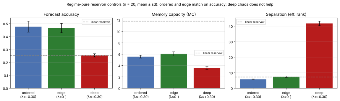
The control does not support a criticality-specific benefit (Table 4, Figure 3). On forecasting under the canonical random-input protocol at seeds, the ordered reservoir reaches (bootstrap 95% CI ) and the edge reservoir , both beating the linear reservoir’s on 20 of 20 seeds (Cliff’s in each case, Wilcoxon ). The ordered arm is not worse than the edge arm; it is slightly better, by a margin the paired bootstrap resolves (paired difference , CI , 14 of 20 seeds, Wilcoxon , Cliff’s ). The deep-chaos arm remains indistinguishable from the linear reservoir (paired difference , CI , Wilcoxon ). The ordering is therefore ordered ≈ edge ≫ deep ≈ linear, not edge ≫ ordered, and the edge holds no privileged position within it.
Table 4.
Regime-pure reservoir control (canonical random-input protocol, forecasting task, seeds). The three chaotic-cell arms are identical except for the -calibration target, so the autonomous exponent is the only deliberately varied quantity. Accuracy intervals are percentile bootstrap 95% CIs on the mean. MC is linear short-term memory capacity; separation is the effective rank of the collected states. The ordered arm matches or slightly exceeds the edge arm on accuracy while both far exceed the linear reservoir; neither diagnostic tracks accuracy. Bold marks the best value in each column.
Standard reservoir diagnostics measured on the same runs sharpen the point rather than rescue the original reading. Linear short-term memory capacity [21] is (ordered), (edge), and (deep), against for the linear reservoir; effective rank, our separation measure in the sense of [20,50], is , , , and , respectively. Neither quantity tracks accuracy. The edge exceeds the ordered arm in memory capacity by only (CI ) while scoring marginally lower in accuracy, and the linear reservoir has roughly twice the memory capacity of any nonlinear arm while performing at chance—so the forecasting advantage is not a memory-capacity effect. Separation is maximized by a wide margin in deep chaos, which confers no advantage at all, so separation without contraction is not usable by a linear readout. What the two surviving arms share is a nonlinear state map operating in a contracting regime, which is what the linear control lacks and what deep chaos destroys. We therefore attribute the reservoir benefit to bounded nonlinear mixing under contraction, not to proximity to the chaos onset, and we have not isolated the nonlinear-transformation component further (Section 4.2).
Figure 3.
Regime-pure reservoir control (mean ± sd over 20 seeds; dashed line = linear reservoir). The three arms differ only in the calibrated autonomous exponent. (Left): forecasting accuracy, where ordered and edge are close and both far exceed the linear reservoir, while deep chaos sits on it. (Center): memory capacity, highest in the linear reservoir, which performs at chance. (Right): separation, highest by far in deep chaos, which confers no advantage. Neither diagnostic is maximized where accuracy is.
A finer axis. Three points establish that the edge is not privileged but do not show the shape of the dependence, so we repeated the sweep at seven calibration targets spanning to , at seeds, with the same diagnostics (Table 5, Figure 4). All seven targets calibrate to within tolerance. The resulting curve is flat and then falls off a cliff. Across the entire stable range, the accuracy is , , , , and at achieved exponents of , , , , and , respectively, with every one of these points beating the linear reservoir on 5 of 5 seeds by between and . Within that plateau, the trend with is weakly negative and not resolved (Spearman , over the 25 runs), and the most ordered point we tested is statistically indistinguishable from the nominal edge (paired difference , 95% CI ). Past the onset, the benefit disappears: at , the mean falls to , and at to , the linear reservoir’s value (paired difference , CI ). Over all seven points, accuracy decreases monotonically with the exponent (Spearman , ). There is no peak anywhere near criticality; there is a plateau that ends at it.
Table 5.
Frozen reservoir along the Lyapunov axis (canonical random-input protocol, forecasting, seeds). Seven calibration targets on the identical cell; all reach the target within tolerance. Intervals are percentile bootstrap 95% CIs, and the comparison against the linear reservoir is paired by seed. Accuracy is flat from to and collapses above it, while separation jumps discontinuously at the same place. Bold marks the best value in each column.
Figure 4.
Frozen reservoir along the Lyapunov axis (mean ± sd over 5 seeds; dashed line = linear reservoir; dotted line = chaos onset; shading marks the stable regime). (Left): forecasting accuracy is flat across the whole stable range and collapses to the linear reservoir’s level only past the onset; the edge holds no peak. (Center): memory capacity rises gently toward the onset but stays far below the linear reservoir, which performs at chance. (Right): separation jumps discontinuously just above the onset, and the wide error bar at reflects seeds falling on either side of that bifurcation rather than sampling noise.
The separation diagnostic locates the cliff precisely, and the mechanism is not subtle. Effective rank is flat and modest across the plateau, rising only from to , and then jumps discontinuously: the individual runs cluster at either 8–10 or 37–44, with nothing in between. That jump coincides exactly with the loss of accuracy. Every run in our sweep with effective rank above 20 () scores on average, indistinguishable from the linear reservoir, and every run below it () averages . The target is where the two coexist: three seeds retain rank – and accuracy –, while two jump to rank and with accuracy and , despite autonomous exponents ( to ) that barely differ. The collapse is therefore not a smooth function of the autonomous exponent at all. It is a bifurcation in the driven reservoir—the state trajectory ceasing to be a contracting function of the input history, so that the echo-state property is lost and the readout is handed a high-rank but input-unreproducible state. This is the same failure mode that Carroll [51] reports as a breakdown of generalized synchronization, observed here as a seed-level bifurcation rather than a trend.
Conditional exponents on the forecasting task. The driven exponents on this task, measured with the same validated Benettin/QR estimator (Section 2.3) on the edge arm at seeds (60-step transient, 240-step accumulation, one driven trajectory per seed; a shorter window than the 100/400 used for the autonomous analysis of Section 3.7, since each seed here requires a separately trained model), also bear on the synchronization account of Section 3.1. Under random input, the conditional exponent averages (sd ), positive on 1 of 20 seeds, against an autonomous value of about : the input drive alone already renders the nominally critical reservoir mildly contracting, which is consistent with its matching the ordered arm. Under trained input, it averages (sd ) and is negative on all 20 seeds, a shift of roughly in the contracting direction attributable to training B. This measures on forecasting the same generalized-synchronization mechanism we report for copy in Section 3.7, and closes the gap left by reporting driven exponents only on the retention tasks.
Finally, the deep-chaos configuration’s non-finite training loss (Table 2) requires an explanation. The triangle fold is bounded onto by construction, and we have verified computationally that neither the fold nor its Jacobian produces non-finite values under the gains and magnitudes used here; we therefore do not attribute the divergence to unbounded state dynamics, as we speculated in an earlier version of this manuscript.
We have since isolated the cause, and it lies in the backward pass rather than in the forward state. We instrumented the trained-input deep-chaos configuration over 12 seeds, recording at every step the training loss, the pre-clipping gradient norm, and the top singular value of the driven-state Jacobian , and we evaluated the forward loss at initialization separately. The forward loss was finite at initialization on every seed, which confirms the bounded-state argument above: no run failed in the forward pass. The gradient, however, failed on all 12 of 12 seeds, with pre-clipping norms reaching .
The discriminating measurement is the driven Jacobian. Its top singular value averages in the deep-chaos arm against in the edge arm, so the deep-chaos recurrence expands along the driven trajectory while the edge arm remains near-isometric. Backpropagation through the 64-step sequence multiplies these expanding Jacobians, and the gradient therefore grows geometrically until it is no longer representable. The divergence is exploding backpropagation-through-time gradients through a genuinely expanding recurrence, and not a loss of boundedness in the state.
Two further observations support this attribution. First, of the standard remedies, only the one that targets the Jacobian product removes the failure: truncating backpropagation to an 8-step window eliminates it entirely (0 of 8 seeds diverge), whereas replacing the triangle fold with a smoothed variant whose derivative is continuous—which removes the shear at the fold kinks but leaves the same 1-Lipschitz bound, and therefore the same expansion—leaves the divergence rate at . Reducing the learning rate to gives , and tightening gradient clipping to gives ; these bound the growth without removing its source. The fold kinks are therefore not the operative mechanism, and the positive conditional expansion is. Second, our instrumented rate is 12 of 12 rather than the 18 of 20 recorded in Table 2, and the difference is one of detection rather than of behavior: clipping by total gradient norm rescales a non-finite norm to zero, so a run whose gradient has already failed can continue with effectively zero updates and still report a finite loss. A loss-level check, which is what produced the 18-of-20 figure, misses such runs, whereas a gradient-level check does not. We retain the originally reported 18 of 20 in Table 2 as the measurement that test performed, and note that the underlying failure rate is effectively total. Figure 5 shows the gradient-norm traces and the mitigation comparison.
Figure 5.
Why the trained-input deep-chaos configuration diverges. (a): pre-clipping gradient norm against training step, one trace per seed; the deep-chaos arm (red) grows geometrically to non-finite values, while the edge arm (green) remains bounded near unity. (b): divergence rate under each mitigation. Only truncated backpropagation, which caps the number of expanding Jacobians multiplied in one gradient, removes the failure; smoothing the fold, which removes the kinks but not the expansion, does not.
We continue to exclude this configuration from our causal comparisons, but we now do so because it is a diagnosed optimization failure of the trained-input protocol at positive conditional exponent, rather than because it is unexplained.
3.2. Generality of the Reservoir Benefit Across Chaotic Maps and Flows
The results above use one chaotic generator: the coupled logistic-fold map. We emphasize at the outset what this sweep does and does not vary: the forecasting target is held fixed throughout—it is the same logistic series () used in Section 3.1—and what changes across the six families is the local nonlinearity inside the reservoir cell. This sweep therefore tests whether the regime ordering is an artifact of the logistic-fold construction; it cannot test whether that ordering depends on the target, because the target does not change. Section 3.3 varies the target instead, and finds that it does. To test whether the canonical-protocol reservoir benefit (Section 3.1) is a property of that specific construction or of the frozen nonlinear reservoir generally, we repeat the frozen-reservoir forecasting comparison across six chaotic reservoir constructions sharing the same surrounding architecture and the same -calibration to a common target exponent: four elementwise maps (logistic, tent, cubic, and sine) and, as the strongest available test, two structurally unrelated continuous ODE flows—the Rössler and Lorenz systems at their classical chaotic parameters (, , for Lorenz; , for Rössler), integrated as recurrent cells as follows. The -dimensional state is partitioned into 21 non-overlapping triples (63 of the 64 dimensions; the one remaining dimension receives no flow contribution and is driven only by the coupling term , exactly as an unused channel would be for the elementwise maps). Each triple is affine-rescaled from into the attractor’s native coordinate range (Lorenz: , , ; Rössler: , ), advanced through four classical Runge–Kutta substeps at (total integration time per recurrent step), and rescaled back; the resulting increment—on the same scale as the elementwise maps’ local contributions—is summed with before the shared -scaling and fold, so the surrounding architecture, including the -calibration procedure, is identical across all six families and does not need to be adapted for the continuous case: acts as the same single scalar expansion control whether the local nonlinearity is a map or an integrated flow. All seeds are reported; we pre-specified that seeds whose gain calibration failed to reach the target exponent band would be excluded, but none did so by that criterion, so no exclusions were applied (Section 3.2).
We ran this comparison with both an ordered arm () and an edge arm () against the matched linear reservoir, at seeds per system under the canonical frozen-input protocol (readout and layer normalization only; the input encoder is frozen, so every arm trains the same 2208 parameters as the single-system fair test of Section 3.1). The result reproduces the single-system control on every system tested (Table 6, Figure 6). Both nonlinear arms beat the linear reservoir (forecasting accuracy ) on all six systems, by to , and the ordered arm is at or above the edge arm throughout: logistic versus , tent versus , cubic versus , sine versus , Rössler versus , and Lorenz versus . Pooling the 30 paired seed differences, the edge arm is below the ordered arm (bootstrap 95% CI , ordered better on 21 of 30 seeds), so across six structurally unrelated systems, the edge holds no advantage over the ordered regime. No run in any arm fell below its linear control, and the cubic and sine collapses seen in an earlier version of this sweep do not recur: that version additionally trained the input encoder, and the collapses were an artifact of the optimizer finding a degenerate input embedding rather than a property of those maps. The generality we can support is therefore a generality across reservoir constructions, on this target: for a one-step-Markov forecasting target, the untrained nonlinear reservoir in a stable-to-critical regime helps regardless of which local nonlinearity it is built from, and the critical regime holds no advantage within it. Section 3.3 shows that this last clause is target-dependent and does not survive a target with long-range structure.
Table 6.
Generality of the canonical-protocol reservoir benefit across six chaotic reservoir constructions (forecasting accuracy, seeds, frozen-input protocol). Chance ; the linear reservoir scores throughout. The paired column is edge minus ordered per seed with a bootstrap 95% CI. Both nonlinear arms beat the linear reservoir on every system, the ordered arm is at or above the edge arm throughout, and no run collapses below the linear control. Bold marks the best value in each column.
Figure 6.
Regime-pure control across six chaotic reservoir constructions (frozen reservoir, canonical random-input protocol, mean ± sd over 5 seeds, frozen input encoder). For every system, the ordered arm () is at or above the edge arm (), and both exceed the linear reservoir (gray) by a clear margin. The two continuous ODE flows (Rössler, Lorenz) give the largest benefits; no arm falls below the linear control on any system.
An earlier version of this manuscript reported a smaller-scale Mackey–Glass pilot here. That pilot has been superseded and is not reported: it predated the protocol correction described in Section 3.1 and trained the scalar input encoder alongside the readout, and it varied only the critical arm, so it could not address the regime question at all. It has been re-run in full under the canonical protocol with ordered, critical, and deep arms and is reported in Section 3.3, where it carries considerably more weight than an external-validity check: it is the target on which the regime ordering reverses.
We restrict this generality claim to the reservoir benefit. We also ran the complementary end-to-end training comparison across the same systems, but do not report it as evidence: in that setting, the arms (including the logistic reference) largely failed to train to non-trivial accuracy, so their Lyapunov exponents describe models that did not learn the task rather than models that learned it while suppressing chaos. The suppression finding of Section 3.6 and Section 3.7 rests on the main experiments, where the arms do train; we do not extend it across systems here.
3.3. When Criticality Does Pay: Task-Matched Memory
Every regime-pure comparison so far has used a single target: next-step forecasting of a logistic series. That leaves one explanation untested, because a property of the task cannot vary when the task is held fixed. We therefore ran the identical frozen arms—same cell, same -calibration, same canonical protocol, 2208 trainable parameters throughout—on two further targets at seeds. The first is the Mackey–Glass delay-differential system at the standard , a continuous, infinite-dimensional-phase-space series of a different character from the discrete maps. The second is a non-chaotic control (a sum of incommensurate sinusoids with mild noise), which tests whether anything here depends on the target being chaotic at all.
On Mackey–Glass, the ordering reverses (Table 7, Figure 7). The critical reservoir reaches against the ordered reservoir’s , a paired difference of (bootstrap 95% CI ) with the critical arm ahead on 5 of 5 seeds—the opposite sign from the logistic control, where the ordered arm led by . Deep chaos reaches and the linear reservoir , so on this target, even deep chaos clears the linear control, which it never does on the logistic task. No run diverged. On the non-chaotic control, everything compresses toward the linear baseline—critical , ordered , linear —and deep chaos actively hurts ( against its own linear control). The claim that the edge holds no privileged position, which the six reservoir constructions of Section 3.2 support on the logistic target, is therefore false in general: it is true of the task we had been testing, not of frozen reservoirs as such.
Table 7.
Frozen reservoirs on two further targets (canonical protocol, seeds, 2208 trainable parameters, no divergences). The paired column is critical minus ordered per seed. On Mackey–Glass, the critical arm leads on 5 of 5 seeds, reversing the ordering found on the logistic target; on the non-chaotic control, all arms compress toward the linear reservoir and deep chaos falls below it. Bold marks the best value in each column.
Figure 7.
Frozen reservoirs on two further targets (mean ± sd, seeds; dashed line = linear reservoir). (Left): on Mackey–Glass, the critical arm leads the ordered one, reversing the ordering of every other comparison in this paper. (Right): on a non-chaotic target, the arms compress toward the linear reservoir and deep chaos falls below it.
Why the ordering depends on the task. Summed memory capacity cannot explain this, since the reservoirs are unchanged between targets; what changes is which part of the past the target depends on. We therefore measured memory capacity resolved by delay—the per-lag whose sum is the usual scalar—on the same frozen arms, with no training involved (Table 8, Figure 8a). The two nonlinear arms are not uniformly ordered. The ordered reservoir retains more than the critical one at lags 1–3 ( in the ordered arm’s favor, consistent on 5 of 5 seeds), and the critical one retains two to three times more at lags 4–12 (, 5 of 5) and marginally more beyond (, 5 of 5). The crossover sits at about lag 4.
Table 8.
Memory capacity by delay band (frozen reservoirs, i.i.d. probe, seeds, no training), against each target’s summed lagged mutual information in the same band. The ordered arm holds more at short delays and the critical arm more from lag 4 onward, each consistently on 5 of 5 seeds; Mackey–Glass is the only target whose demand is concentrated where the critical arm leads. Bold marks the best value in each column.
Figure 8.
Why the ordering depends on the target. (a) Memory capacity resolved by delay (mean ± sd, 5 seeds, no training): the ordered arm holds more at lags 1–3, the critical arm two to three times more at lags 4–12 (shaded), and the linear reservoir more than either everywhere. (b) Lagged mutual information between and : the logistic target collapses after a few steps while Mackey–Glass shows a second peak near lag 22, the signature of its delay. (c) Across three targets, the critical arm’s margin over the ordered one tracks long-lag demand monotonically, changing sign; error bars are bootstrap 95% CIs, and the three are mutually disjoint.
The targets differ in exactly the way that makes this matter (Figure 8b). Lagged mutual information between and collapses for the logistic map— nats by lag 12 and flat thereafter, as expected of a one-step Markov system—whereas Mackey–Glass falls to a trough near lag 11 and then rises to a second peak of nats at lag , the signature of its delay. Summed over the band where the critical reservoir holds the advantage (lags 4–12), Mackey–Glass demands what the logistic map does; beyond lag 13, it demands . The critical arm’s extra memory is worthless on a target that reaches back three steps and valuable on one that reaches back twenty.
Across the three targets of this section, the critical arm’s margin tracks that demand monotonically (Figure 8c; Section 3.4 extends this to six targets): (CI , ) on the logistic map at a long-lag demand of nats, (CI ) on the non-chaotic control at , and (CI ) on Mackey–Glass at . The three intervals are mutually disjoint and the ordering is strict, including the change of sign.
We are explicit that memory alone does not predict performance, and we tested this rather than assuming it. Scoring each reservoir by the overlap between what it retains and what the target needs, , fails to rank the arms (Spearman ): the linear reservoir scores highest on every target, retaining even at lag 8 and a summed capacity of against the critical arm’s , and performs at chance regardless. What survives is a two-factor account. Bounded nonlinearity under contraction is necessary: the linear reservoir has the memory and lacks the nonlinearity, while deep chaos has the nonlinearity and the worst memory of any arm () together with a driven state that is no longer a contracting function of its input. Given that necessary condition, the regime that wins is the one whose memory profile matches the target’s reach. Criticality is not a privileged operating point; it is simply the point, among those we tested, that holds memory furthest back while still contracting.
Three caveats bound this account. It rests on three target points, not on the six reservoir constructions of Section 3.2, which hold the task fixed and therefore cannot test it; with targets, the monotone ordering and the disjoint intervals are suggestive but far from a demonstrated law. Mackey–Glass’s strongest dependence, at lags 17–25, lies beyond what either nonlinear reservoir retains—both sit at the noise floor there—so the critical arm’s advantage comes entirely from the 4–12 band rather than from exploiting the delay peak itself. And the account is a mechanism consistent with all of our measurements and making a falsifiable prediction—that the critical arm’s advantage should appear and disappear with a target’s long-lag structure, at a crossover near lag 4 for this cell—not a result we have established across task families.
3.4. Robustness and Direct Diagnostics
The account above rests on a specific reservoir, a specific readout, a specific set of targets, and a training-time Lyapunov estimate. This section reports five controls that test each of those choices directly.
Standard benchmarks and graded memory demand. The two-factor account of Section 3.3 rested on three targets, and we noted that a proper test would sweep targets of graded memory demand. We have now done so. We repeated the canonical frozen-reservoir comparison on two standard reservoir-computing benchmarks (NARMA10 and NARMA30 [52]), on a real measured series (the Santa Fe laser data of Weigend and Gershenfeld [53]), and on the three targets already reported, adding a leaky-integrator echo-state network [54] as a further baseline; every arm carries the same 2208 trainable readout parameters. Table 9 gives the benchmark results. Across all six targets, the critical arm’s margin over the ordered arm tracks the target’s measured memory demand—the mean lagged mutual information between the target and its driving history over lags , defined in Section 2.4—with a Pearson correlation of (; Spearman ), ordered from NARMA10 at demand and margin through the Santa Fe laser at demand and margin to Mackey–Glass at demand and margin , and changing sign on the logistic target, whose demand is lowest among the chaotic series. Figure 9 shows the relationship.
Table 9.
Frozen reservoirs on standard reservoir-computing benchmarks and a real measured series (canonical protocol, seeds, 2208 trainable parameters). “Margin” is the paired edge-minus-ordered accuracy difference with a bootstrap 95% confidence interval; demand is the mean lagged mutual information with the driving history over lags (Section 2.4). Bold marks the best value in each column.
Figure 9.
The critical arm’s margin tracks the target’s measured memory demand across six targets. Each point is one target; the horizontal axis is the lagged mutual information between the target and the input history, and the vertical axis is the paired edge-minus-ordered accuracy margin. The relationship is monotone in demand and changes sign at low demand (Pearson , ).
One result in this sweep deserves to be stated plainly, because it did not come out as we expected. NARMA30 is constructed with a deeper designed memory than NARMA10, so on a reading in which designed depth drives the ordering, it should show the larger critical margin. It does not: both NARMA margins are statistically indistinguishable from zero ( and ), and both arms sit near the accuracy floor on these targets. The reason is that NARMA is driven by independent uniform noise, which keeps the mutual information between the target and the input history low however deep the recurrence in the target’s definition. It is therefore the measured demand, and not the designed memory depth, that is the operative variable, and we report the correlation on that basis rather than on the designed one. We note that this is also a limitation of NARMA as a probe of the present hypothesis.
The ordering does not depend on how the readout is fit. Because the readout is the only trained component under the canonical protocol, a result could in principle reflect readout optimization rather than reservoir quality. We therefore refit every arm with a closed-form ridge readout on the same frozen features, in place of the gradient-descent readout used throughout. The ordering of the three regime-matched chaotic arms is identical under the two methods (Spearman ), as Table 10 shows, so the result is not an artifact of how the readout is optimized; across all five arms, the two readouts agree at , the single inversion being the deep-chaos and linear controls, which sit within of one another under both methods and far below the ordered and edge arms under either. The same table reinforces a point made in Section 3.1: among the three chaotic arms, the effective rank of the frozen features is anticorrelated with accuracy (Spearman ), with deep chaos carrying by far the richest representation ( against for the ordered arm) and the lowest accuracy of the three. Separation, measured this way, does not track usable computation.
Table 10.
The arm ordering is the same under a closed-form ridge readout and the gradient-descent readout (canonical protocol, forecasting target). Effective rank is the participation ratio of the frozen features; MC is the delay-summed memory capacity. Bold marks the best value in each column.
A direct synchronization diagnostic. Section 3.1 attributes the collapse past the chaos onset to a loss of the echo-state property, inferred from the conditional exponent. We have now measured it directly with the auxiliary-system, or replica, test: two copies of the same frozen reservoir, identical in every parameter, are driven by the same input sequence from different random initial states, and we record the normalized asymptotic discrepancy after a washout. If the reservoir’s state is a function of its input history alone, the two trajectories must converge and . They do, exactly, at every stable calibration from to ( at all five points, all seeds), and they fail to converge past the onset ( at and at ). Figure 10 shows the step. This is an independent confirmation of the echo-state reading, obtained without reference to any Lyapunov estimator.
Figure 10.
A direct auxiliary-system test of the echo-state property. (a): the normalized asymptotic discrepancy D between two identically parameterized reservoirs driven by the same input from different initial states, against the achieved autonomous exponent. D is exactly zero at every stable calibration and becomes positive only past the chaos onset. (b): the same quantity at the three named regimes under random and trained input; the deep-chaos trained bar reflects an input projection that could not train (Section 3.1) and should not be read as a trained condition.
We add one caveat about the trained-input condition in that measurement, which we state rather than gloss. For the ordered and edge calibrations, training the input projection leaves D at zero, as expected. For the deep-chaos calibration, D is essentially unchanged by training ( under random input against under trained input), but this should not be read as a trained condition that fails to synchronize: it is the same gradient failure diagnosed in Section 3.1, which that measurement’s loss-level check did not detect, so the input projection in fact made no progress, and the trained bar is effectively the random-input one. The ordered and edge columns carry the interpretable content.
The ordering survives changes to width, normalization, readout, and depth. We varied each of these one at a time around the reported configuration (, layer-normalized features, ridge readout, a single reservoir layer) and re-measured all four arms with five seeds. Across all seven architectural variants, the two load-bearing orderings hold without exception: the edge reservoir beats the matched linear reservoir (margins from to ) and beats the deep-chaos arm (from to ), and in every variant, the ordered arm is at or above the edge arm (from to ), so criticality holds no privileged position under any of them. Figure 11 shows the variants and the three diagnostic gaps. Two features of the sweep are worth noting. First, the separation strengthens with capacity rather than washing out: at , the edge-over-linear and edge-over-deep margins widen to and . Second, giving the readout its own nonlinearity does not rescue either control: with a one-hidden-layer readout, the linear reservoir improves substantially to , but the edge reservoir still leads it by and still leads deep chaos by . At depth two, the deep-chaos arm falls to , below the linear control’s , which is consistent with stacking two expanding reservoirs compounding the loss of the echo-state property.
Figure 11.
The frozen-reservoir ordering is robust to width, normalization, readout, and depth. (a): accuracy of the four arms across the seven architectural variants. (b): the three diagnostic gaps. Edge exceeds linear and edge exceeds deep chaos in every variant, and the ordered arm is at or above the edge arm in every variant.
The windowed training proxy, dissected. Section 3.7 reports that the windowed proxy used as a training signal overestimates the validated conditional exponent. We can now say by how much, and why it cannot be fixed by tuning the window alone. Let along the driven trajectory. Because , the sequence is subadditive, and Fekete’s lemma gives ; the windowed estimate is therefore an upper bound on the true exponent at every finite W, and can only ever overestimate. Measured on the gated cell across a range of gains spanning to , the mean bias is at and decays monotonically to at (the window used for training), at , and at . The bias is far larger at the chaotic gains than at the ordered one— at against to across the positive-exponent gains, with its maximum of falling at rather than at the largest exponent—and at the ordered gain, the single-step proxy reports against a true exponent of , so a genuinely contracting system is reported as only about half as contracting as it is. Figure 12 shows both the bias and its decay.
Figure 12.
The windowed Lyapunov proxy overestimates at every window length. (a): the proxy against the validated conditional exponent for several window lengths W; every curve lies above the diagonal, descending toward it as W grows. (b): the mean bias against W, decaying from at to at . Subadditivity makes the overestimate a guarantee rather than an empirical accident.
The constructive half of this control is that an unbiased alternative exists and is differentiable. The long-horizon Benettin/QR accumulation is autograd-compatible, and, implemented that way, it recovers the validated exponent to within across all gains while retaining a finite and strictly positive gradient with respect to the gain parameter (per-gain mean between and , and positive on every individual run). A long-horizon differentiable estimator is therefore available as a training objective in place of the short-window proxy, which is the strengthening we identified as future work in Section 4.2; we report it here as an available instrument rather than as a retrained result, since replacing the training signal would change the corridor experiment rather than control it.
3.5. The Chaotic Recurrence Confers No Benefit and Is Not Trainable to Ceiling
Having established a regime in which the frozen recurrence performs well above its controls, we now turn to the setting this paper set out to test: the same recurrence trained end to end. The remainder of this section reports that it confers no benefit there, identifies the mechanism, and shows the mechanism is not a tuning artifact. On a working harness—the same pre-norm residual block for every arm, trained to convergence—a GRU solves the 12-token copy task essentially perfectly ( held-out accuracy over eight seeds), confirming the task and harness are sound. Under identical conditions, neither chaotic variant approaches this ceiling: the free chaotic arm reaches and the corridor-regularized arm , while the diagonal selective-SSM reaches and the linear arm (Table 11, Figure 13). The separation between the GRU and every other arm is complete (Cliff’s delta of unity), and the chaotic arms sit far below a model that trivially solves the task. Moreover, a learning-rate sweep does not rescue them, and both chaotic arms diverge at the highest sweep rate. This is a major concern for the hypothesis, since it indicates that the chaotic parameterization is harder to optimize, not richer in usable capacity; note in particular that divergence under an increased learning rate is evidence of an optimization ceiling rather than of simple under-training, which would instead be relieved by a larger step or budget. Parameter count does not explain the gap: the chaotic arms carry the same budget as the linear control (58.3k versus 58.2k at ) and only about 14% less than the GRU (Table 1), yet sit at a fraction of its accuracy. The selective-SSM’s own shortfall relative to the GRU is consistent with prior reports that pure state-space models trail gated recurrent and attention-based architectures specifically on tasks requiring strong copying [4]; we did not separately tune this baseline beyond the documented sweep, and offer it as a reference point rather than a load-bearing comparison.
Table 11.
Held-out copy accuracy on the fixed harness (mean ± sd, ). Chance . A GRU reaches ceiling; the chaotic arms do not approach it. The GRU-versus-others separation is complete (Cliff’s , i.e., non-overlapping seed distributions); standard deviations are shown for every arm.
Figure 13.
Held-out accuracy across arms on the fixed harness (copy task, mean ± sd over 8 seeds; dashed line = chance). The GRU reaches ceiling while both chaotic arms remain near the floor, well below the diagonal selective-SSM.
3.6. Chaos Is Not the Causal Variable: The Periodic-Regime Ablation
It might still be objected that the chaotic arms’ weak behavior nonetheless reflects some contribution from chaos. We test this with a controlled causal ablation: we cap the logistic rate below the chaos onset so the map is confined to fixed-point and periodic dynamics, changing exactly one scalar and holding every other parameter, initialization, and code path identical. If chaos contributes anything, the chaotic-rate arm should beat its periodic-rate twin. However, it does not. Across copy and selective copy, and for both the free and corridor families, the periodic variant matches or slightly exceeds the chaotic variant, with every Cliff’s delta negative and, on the copy/corridor comparison, a bootstrap confidence interval lying entirely below zero (Table 12, Figure 14). We flag a scope limit on this comparison explicitly, applying the same skepticism we apply to Table 2: both arms sit near the chance floor (Table 11), so the accuracy deltas in Table 12 are themselves small in absolute terms. What makes this comparison interpretable despite the floor is its design, not its magnitude: the chaotic-rate and periodic-rate arms are identical in every parameter, initialization, and code path except the single scalar rate cap, so any systematic difference between them is attributable to that scalar rather than to overall task difficulty, which is shared. Whatever the chaotic arms achieve is therefore attributable to their nonlinearity and parameterization, not to chaos; confining the map to the periodic regime is, if anything, marginally better than allowing it to be chaotic. We do not draw the same causal conclusion from unpaired floor-level comparisons across different architectures (e.g., Table 2), where task difficulty is not held fixed by design.
Table 12.
Periodic-regime ablation (mean held-out accuracy, ). The periodic-r twin matches or beats the chaotic-r arm on every task; positive “chaos helps” nowhere.
Figure 14.
Periodic-regime ablation. For each task and family, held-out accuracy of the chaotic-rate arm and its periodic-rate twin, with GRU and linear controls (mean with bootstrap 95% CI over 8 seeds). All differences are at or below zero; on the copy/corridor comparison, the interval lies entirely below zero.
The same ablation at graded dependency length. The comparisons above run on short synthetic sequences near the accuracy floor, which leaves open whether the conclusion that chaos confers no advantage is an artifact of that floor. We therefore repeated the chaotic-versus-periodic ablation on a delay-recall task in which the required dependency length is a directly controlled parameter: a content token is presented, followed by D padding positions, a query cue, and a separator, and the model must emit the content at the final position. We sweep with five seeds, against a GRU and a linear control, with the chaotic arm and its periodic twin again identical in every trained parameter except the rate cap ( parameters each).
This task is not at a floor, which is what makes the comparison informative. At , 12, and 24, every arm except the linear control reaches perfect accuracy, while the linear control collapses at () and (), confirming that the task genuinely requires retention rather than rewarding a shortcut. The arms separate at : the GRU still solves it perfectly (), the periodic twin reaches , the chaotic arm reaches , and the linear control sits at the floor. The paired periodic-minus-chaotic advantage at is (95% CI ), with the periodic twin ahead on 5 of 5 seeds; Figure 15 shows the full sweep. The conclusion therefore does not merely survive a longer dependency; it sharpens: at the longest dependency, the chaotic recurrence is not neutral but substantially worse than the identical non-chaotic control, which is the opposite of what the edge-of-chaos hypothesis predicts for a task requiring long retention.
Figure 15.
The periodic-regime ablation at graded dependency length. Held-out accuracy on the delay-recall task against the required delay D (mean over 5 seeds). All arms except the linear control are at ceiling through ; at , the chaotic arm falls well below its matched periodic twin, which is identical in every trained parameter except the rate cap, while the GRU remains at ceiling and the linear control sits at the floor throughout the longer delays.
The conditional exponent locates where the two arms part company. At , 12, and 24, both gated arms drive the measured conditional exponent to exactly zero on every seed: the gate closes completely, leaving the recurrence an identity map along the driven trajectory, which is the contraction mechanism of Section 3.7 operating exactly as described there. At , the gate no longer closes. The chaotic arm’s conditional exponent then averages and is positive on all five seeds, while the periodic twin’s averages and is negative on two of five; the arm that remains expanding along its own task input is the arm that fails. We state one limit on this reading explicitly: within the chaotic arm, the per-seed correlation between the conditional exponent and accuracy at is essentially zero (Pearson , ), so this is a between-arm contrast and not a within-arm dose–response, which five seeds could not establish in any case.
3.7. The Mechanism: Trained Models Contract On-Task, and the Gate Is Responsible
To understand why, we measure the conditional Lyapunov exponent of the trained models along their real task inputs, and contrast it with the map’s autonomous capacity for chaos. The conditional exponent is the quantity that governs the driven model’s behavior. We report both exponents for the trained parameters in Table 13, and we are careful to state precisely what they show: the autonomous exponent of the trained parameters is itself negative for every arm, so the trained models are not, in fact, chaotic even in the absence of input. Positive autonomous exponents are reachable by the underlying map only under the gate-open manipulation of Table 14 (Section 3.7), which alters the recurrence rather than merely re-measuring the trained one. The correct statement is therefore that training suppresses chaos along two related but distinct axes—the trained autonomous dynamics and the driven conditional dynamics are both contracting—and that forcing the gate open on the trained parameters is what reveals the map retains the capacity for positive exponents. Across every arm and seed, including the free chaotic arm that is allowed a rate cap deep in the chaotic regime, the conditional exponent is negative (Table 13): the trained models operate in a contracting regime on-task even when the map is free to be chaotic. Two controls bound this result. Recomputing the exponent with a fresh input drawn independently for each trajectory, rather than a single reused trajectory, changes it by about and leaves it negative on every seed, ruling out a reuse artifact; and the autonomous (undriven) and random-drive exponents of the same trained parameters are likewise negative (Table 13), so the contraction is a property of the learned parameters and gate, not of one particular drive. We note that the random-drive exponent is consistently more negative than the conditional (real-input) exponent: unstructured noise contracts the recurrence more strongly than structured task input does. This is consistent with the gate contracting in response to any nonzero input rather than to task structure specifically, while real inputs, carrying temporal structure the model partially tracks, leave slightly more expansion than white noise. Notably, the windowed training proxy the corridor regularizer optimizes reports the opposite sign (Figure 16): it indicates expansion for the same models the validated estimator finds contracting, which explains why regularizing the proxy toward a positive corridor does not make the trained recurrence chaotic on-task.
Table 13.
Lyapunov exponents of trained models (mean over 5 seeds; sd shown for the primary, conditional estimate). The conditional (driven-real) exponent is negative for every arm; the autonomous (undriven) and random-drive controls are likewise negative for the trained parameters, and the windowed training proxy reports the opposite sign. The map’s capacity for positive exponents under these same trained parameters is demonstrated by the gate-open condition of Table 14. Standard deviations are reported only for the conditional exponent, the primary validated estimate on which our causal claims rest and the only one we use in a quantitative comparison elsewhere in this paper. The autonomous, random-drive, and proxy columns are secondary controls, collected and retained as per-arm means; we did not additionally retain per-seed dispersion for these three, and report this as a limitation rather than assert a robustness we have not measured.
Table 14.
Gate dose–response: conditional of the trained free chaotic model as the gate is forced open (mean over 5 seeds). Opening the gate restores positive Lyapunov exponents.
Figure 16.
The windowed training proxy overestimates the true conditional Lyapunov exponent. Each point is one trained model (5 seeds × 4 arms); the x-axis is the validated conditional exponent (Benettin/QR, driven by real task inputs), and the y-axis is the training proxy. Every point lies far above the line: the proxy reports expansion (positive) where the validated estimate reports contraction (negative), which is why the corridor regularizer, steering by the proxy, does not prevent on-task contraction.
Moreover, the gap between the contracting on-task dynamics and the map’s capacity for expansion points directly to the gate. We test this by recomputing the conditional exponent of the trained free chaotic model while forcing the gate to fixed values, sweeping from the learned gate to fully open. The result is a clean monotone dose–response (Table 14, Figure 17): with the learned gate, the exponent is , but as the gate opens, the exponent rises, crossing zero near and reaching when the gate is fully open. The map is genuinely capable of chaos; the trained gate holds the recurrence in contraction by mixing in the previous state through its path. One caveat bounds the causal reading: forcing the gate to a fixed value also changes the visited state distribution, so part of the exponent shift may reflect trajectory redistribution rather than the mixing path alone. The monotone dose–response across four gate levels, identical in the free and corridor families, is most parsimoniously explained by the mixing path, but a full gate-family ablation would be required to isolate it completely. End-to-end training does not fail to find chaos—it actively learns to suppress the chaos the map can produce. This mechanism, however, is specific to the gated architecture; we test its generality directly by training the same chaotic map end to end with the gate and skip path removed entirely, so chaos is the only recurrent path available. The result is a second, complementary failure mode rather than a confirmation of the same one. The ungated chaotic arm does not suppress its chaos—its conditional exponent remains solidly positive after training ( on copy, on forecast)—but nor does it solve either task: held-out accuracy is on copy, at the chance floor, and on forecast, below the majority-class baseline, with a divergence rate across seeds. Without a skip path to fall back on, gradient descent does not learn to suppress chaos; it appears unable to find a stable, task-solving configuration at all. We read this as reinforcing rather than undermining this paper’s central claim, via a different route: whether or not an escape path is available, end-to-end training on these tasks does not yield a working chaotic model. Where a skip path exists, training suppresses chaos and partially solves the task (Table 11); where none exists, chaos persists but training fails to stabilize around it. The gate-suppression mechanism of this section should accordingly be read as specific to gated, residual chaotic recurrences, not as a claim about end-to-end training of chaotic recurrences in general.
Figure 17.
Gate dose–response (the central mechanism figure). Conditional Lyapunov exponent of the trained chaotic models as the input gate is forced from its learned value to fully open (mean over 5 seeds; dashed line = chaos threshold, ). The map is capable of chaos ( reaches when the gate is open), but the learned gate holds the recurrence in contraction (), crossing into chaos only near .
4. Discussion
Our results are consistent, and they point to a sharper conclusion than a simple failure of the edge-of-chaos hypothesis: the hypothesis is right that the recurrence must stay untrained, wrong that what it must supply is chaos, and incomplete in a way our later experiments fill in: what it must supply is bounded nonlinearity under contraction, and which such recurrence is best is a property of the task rather than of the reservoir. Three observations, taken together, explain the pattern. First, the reservoir-computing results that motivate the intuition concern fixed random recurrences read out by a trained linear layer, and the richness is a property of the untrained reservoir: our canonical random-input fair test (Section 3.1) shows a frozen nonlinear reservoir nearly doubling a linear reservoir’s accuracy on a chaos-congenial task. The regime-pure control, however, locates that benefit in the ordered as much as the critical regime on that target and shows it absent deep in chaos, so what the classical account predicts is confirmed only in part: the untrained nonlinear reservoir earns its keep, and the edge earns its keep only where the target reaches back far enough to need the memory it holds (Section 3.3). However, the moment gradient descent can modify the recurrence, it optimizes for task loss; and for the memory-like tasks that dominate sequence modeling, task loss rewards stable, reproducible state—precisely the opposite of sensitive dependence. Our gate dose–response is a direct picture of this: the network is handed a map with autonomous chaotic capacity and learns a gate that holds the driven recurrence in contraction, so that the conditional exponent turns negative even though the autonomous capacity remains, consistent with theoretical work showing gating can control the onset of chaos in recurrent networks [55] and empirical work showing driven input can suppress otherwise chaotic recurrent dynamics [56]. The phenomenon is best described as an optimization-induced, input-conditioned contraction (a form of driven synchronization) rather than a removal of chaos from the map itself. Second, there is a tension between sensitivity and precise retention. A positive Lyapunov exponent means nearby input histories diverge exponentially, which is hard to reconcile with the faithful long-range retention that copy and selective copy require. We do not claim chaos and memory are incompatible in general—chaotic systems can support structured transient memory, generalized synchronization, and useful reservoir computation—only that, for the retention-heavy tasks studied here, strong positive exponents work against the required stability. Third, the benefit is fragile in a specific and diagnostic way: it survives freezing the recurrence but not training the input pathway. Training only the input projection B, with the recurrence still entirely frozen, is sufficient to erase the advantage through generalized synchronization [49]—the optimizer maps inputs directly onto the reservoir’s dynamics, collapsing the separation a chaotic map would otherwise provide. This is a second, independent mechanism by which trainability removes the benefit of chaos, distinct from the gated skip path of Section 3.7: one operates on the input pathway of an otherwise fixed reservoir, the other on the recurrence itself once it is also allowed to train. Both point in the same direction: any pathway gradient descent can use to route around or synchronize away from chaotic dynamics, it will use, for tasks of the retention-heavy kind studied here.
These findings should be read with their scope in mind. They concern learnable chaotic recurrences of the gated, input-conditioned form studied here, at the small-to-moderate scale of controlled synthetic tasks, below the long-range benchmark scale [57] at which sequence-model claims are usually contested, and they do not exclude the possibility that chaotic dynamics confer benefits in other settings, and recent work demonstrates settings where they do: chaotic dynamics exploited directly as computational substrates [58] and chaotic neural dynamics serving probabilistic computation through sampling [59]. A further, long-established example is metaheuristic optimization, where chaotic maps—including the logistic and tent maps we use as recurrent-cell generators in Section 3.2—are routinely embedded in bio-inspired search algorithms to diversify exploration and help avoid premature convergence, as in recent chaos-enhanced variants of cuckoo search [60], secretary bird optimization [61], and the chaotic crayfish optimization algorithm [62]. All of these operate in regimes deliberately unlike ours—the chaos is exploited as a fixed search heuristic rather than trained through as a recurrence’s own dynamics—which is precisely the boundary our results draw: it is end-to-end optimization on retention-style sequence tasks, not chaos as such, that our findings speak against. What our results do establish, within their scope, is that the specific and appealing move of replacing a linear SSM recurrence with a trained chaotic one, and regularizing it toward criticality, does not deliver the benefits the edge-of-chaos hypothesis suggests when the recurrence (and, as we additionally show, even just the input pathway) is allowed to train—and that the reason is structural rather than incidental: training drives the conditional Lyapunov exponent negative through input-induced contraction or synchronization. This is not, however, a failure of chaos: our canonical-protocol fair test shows the same class of chaotic dynamics delivers a substantial, theory-predicted benefit when genuinely preserved untrained. The cautionary result is specifically for architecture design that trains a chaotic recurrence, or its input pathway, end to end. It also complements the stability picture of Halloran et al. [2], who bound Mamba-style recurrences to . This is a major point, since it means the confinement to the ordered regime is not merely an artifact of the linear parameterization: we show that even when an architecture is deliberately built to escape that confinement, end-to-end training returns it to the ordered regime of its own accord.
Finally, a minor observation warrants a single sentence rather than a research program: the small above-linear differences on the copy floor suggest the chaotic parameterization alters the learned representation in some measurable way, but not one that improves task accuracy, and we do not interpret it further.
Relation to reservoir-computing theory. It is worth being explicit about where this leaves our result relative to the literature that motivated the study, because the correction is narrower than it may first appear. The claim we withdraw is that the benefit is specific to criticality; the claim we retain—that an untrained nonlinear reservoir substantially outperforms a linear one, and that training the input pathway destroys the advantage—is squarely within reservoir-computing orthodoxy. Standard echo-state networks are in fact operated in the contracting regime: the spectral radius is conventionally scaled below unity to secure the echo-state property, and although that criterion is neither necessary nor strictly sufficient [63], it is what practice follows, so our ordered arm is closer to a conventional reservoir than our edge arm is. Our finding that the edge holds no privileged position also has direct precedent. Carroll [51] asks exactly this question of reservoir computers and exhibits cases in which computational capacity decreases as the edge of stability is approached, in one instance because generalized synchronization breaks down—the same mechanism we measure here when the input projection is trained—and concludes that the edge is not in general an optimal operating point. The evidence is genuinely mixed rather than one-sided: others report accuracy peaking at dynamical phase boundaries in some tasks while finding that chaotic dynamics degrade performance, and that usefully nonlinear computation survives even at severely reduced nonlinearity [64]. Our contribution to this question is methodological as much as empirical: because the arms differ only in a calibrated exponent, the comparison isolates the regime in a way that comparing a chaotic reservoir against a linear one cannot, and the seven-point sweep shows the dependence is a plateau terminating at the onset rather than a peak located on it. The target-varying experiment of Section 3.3 also suggests why this literature disagrees with itself: if the regime ordering depends on the target’s memory demand rather than on the reservoir, then work using short-memory benchmarks and work using delay systems should reach opposite conclusions about criticality while each is correct about its own setting.
The diagnostics admit the same reading. That our linear reservoir has roughly twice the memory capacity of any nonlinear arm while performing at chance is the memory–nonlinearity trade-off in its plainest form [50]: nonlinear dynamics degrade stored memory, and a task that demands nonlinear transformation is therefore not won by the reservoir with the most memory [65].
We should be explicit about what our account adds to this literature, since the matching idea is adjacent to both strands. Dambre et al. [50] show that a reservoir’s total processing capacity is conserved and decomposes into linear and nonlinear components, and Inubushi and Yoshimura [65] show that memory and nonlinearity trade against one another. Both results characterize what a reservoir can compute, as a property of the reservoir itself. They do not say which of several reservoirs that all satisfy bounded nonlinearity under contraction will win on a given target, and that is the question the two-factor account answers. Moreover, our claim is not that capacity is the operative quantity. The natural capacity-style score—the overlap between what a reservoir retains at each lag and what the target demands at that lag—fails to rank our arms (Spearman ), precisely because the linear reservoir maximizes retention and still performs at chance. What ranks them is the delay-resolved match between retention and demand, evaluated only among arms that already clear the nonlinearity condition; this is a two-factor statement rather than a single conserved quantity. Finally, neither result speaks to the regime axis. That an ordered reservoir matches or exceeds a critical one and that criticality pays only when the target reaches further back than the ordered regime retains do not follow from capacity conservation or from the memory–nonlinearity trade-off, and they are what our regime-pure controls and the six-target demand sweep of Section 3.4 establish.
Our forecasting task is of that kind, which is why memory capacity anticorrelates with accuracy across our arms rather than tracking it. The conditional exponent plays the role the same literature assigns it, as the quantity governing generalized synchronization between drive and reservoir and, through it, the memory the reservoir retains [66]; our measurement of it falling to under a trained input projection is a direct instance. What we add is the observation that, in this family, the benefit is not recovered by moving toward criticality, and that separation—maximized by a wide margin in deep chaos—is not usable by a linear readout without contraction to stabilize it. The sweep sharpens this into a criterion: across all 35 reservoir runs, effective rank above 20 predicts chance-level accuracy without exception, and the quantity that matters is therefore not how much the reservoir separates inputs but whether it still does so reproducibly under drive. The delay-resolved analysis of Section 3.3 adds the complementary half: summed memory capacity is not merely an imperfect predictor of accuracy but an actively misleading one, since the linear reservoir maximizes it and performs at chance, whereas memory resolved by delay and read against the target’s own lagged dependence tracks the margin across our six targets (Pearson ), including the change of sign. Reporting the memory-capacity curve rather than its sum is, we would suggest, the cheapest methodological improvement available to this literature.
4.1. Relation to State-Space Model Stability Theory
Our gate dose–response suggests a complementary reading of the non-positive Lyapunov bound that Halloran et al. [2] prove for Mamba-style recurrences. That bound is usually understood as a property of the linear parameterization: a linear recurrence cannot expand, so its maximal exponent is non-positive by construction. Our results indicate that the confinement to is not solely a consequence of linearity. When we remove the linearity constraint entirely—giving the recurrence a map with autonomous chaotic capacity—end-to-end training on retention-style tasks nonetheless drives the conditional exponent negative, voluntarily, through the input gate. On this reading, the stability bound is at least partly emergent from what the task and the optimizer prefer, rather than imposed by the architecture. This is a stronger statement about task structure than the architectural bound alone: it suggests that even an SSM designed to be able to leave the ordered regime would be returned to it by training on the kinds of retention tasks these models are built for. We offer this as an interpretation consistent with our evidence rather than a proof; establishing it in general would require analyzing the optimizer’s preferred fixed points for these dynamics, which is beyond our scope.
4.2. Limitations
Our study is a controlled laboratory investigation, and its scope should be read accordingly. The findings concern a single architectural family—a gated, input-conditioned triangle-fold chaotic cell—at state sizes of 48 to 64, on a small set of synthetic sequence tasks chosen to isolate specific behaviors rather than to represent the full range of sequence modeling. The delay-recall sweep of Section 3.6 extends the trained-setting comparison to a controlled dependency length of up to 48 steps, and shows the chaotic arm falling further behind its non-chaotic twin as that length grows rather than catching up; the tasks nevertheless remain synthetic, and this sweep bounds dependency length rather than task realism. We do not evaluate at the long-range-benchmark or language-model scale at which architectural claims are ultimately contested [57]. Recent work independently exhibits other settings where chaos is computationally useful when exploited rather than trained through [58,59], which our own random-input reservoir result now joins directly rather than merely gestures toward. Accordingly, our negative result—that end-to-end training of the chaotic cell does not preserve a useful chaotic regime—is scoped to this architecture and task family (gated, input-conditioned cells trained on retention-style and forecasting tasks), and we do not claim that no trainable chaotic recurrence could succeed. Seven specific caveats bound our claims. First, the corridor-regularization result is entangled with proxy bias, as discussed in Section 2.2. Second, the fair test’s flagship random-input comparison is now properly powered at (Cliff’s , bootstrap 95% CI ), scaled up from an initial , symmetrically across every condition rather than selectively; the trained-input deep-chaos configuration, however, remains unusable, diverging on 18 of 20 seeds, which we now diagnose as exploding backpropagation-through-time gradients through an expanding recurrence (Section 3.1). Third, the gate dose–response, while monotone and consistent across families, does not fully isolate the state-mixing path from trajectory redistribution (Section 3.7). Fourth, the deep-chaos configuration’s non-finite training loss is now diagnosed (Section 3.1), but the diagnosis is scoped to the trained-input protocol at positive conditional exponent and to backpropagation through sequences of this length; we have not established how the failure threshold moves with sequence length or optimizer. Fifth, the regime-pure control establishes that the reservoir benefit is not specific to criticality, but it does not identify which property of the bounded nonlinear map supplies it. A full information-processing-capacity decomposition [50] into linear and nonlinear components is the natural next measurement; we have not carried it out here. Sixth, and most important for how the two-factor account of Section 3.3 should be read, that account rests on three targets. The six families of Section 3.2 hold the target fixed and therefore cannot test it, so the monotone ordering and the mutually disjoint intervals we report come from three points, one of which carries seeds and two . We regard it as a mechanism consistent with every measurement we have and making a falsifiable prediction—that the critical arm’s advantage should track a target’s long-lag structure, with a crossover near lag 4 for this cell—rather than as an established law, and we would expect a proper test to sweep targets of graded memory demand. Section 3.4 now supplies such a sweep over six targets, in which the margin tracks measured demand at ; this strengthens the account from three points to six, but the targets remain a convenience sample rather than a designed continuum, and the two NARMA benchmarks sit near the accuracy floor. Seventh, Mackey–Glass’s strongest dependence lies at lags 17–25, beyond what either nonlinear reservoir retains, so the critical arm’s advantage there comes from the 4–12 band and not from exploiting the delay peak itself; a reservoir with longer memory might behave differently, and we have not built one. Each of these points to a concrete strengthening. Two of them are now supplied: the numerical divergence is diagnosed (Section 3.1), and a differentiable long-horizon estimator is demonstrated to recover the validated exponent to within with a finite gain gradient (Section 3.4), though we report it as an available instrument rather than retraining the corridor experiment around it. The remainder—additional seeds, a full gate-family ablation, and a designed continuum of memory demand—we leave to future work, none of which alters the converging-evidence structure of the present result within its stated scope.
5. Conclusions
We set out to test a well-motivated hypothesis—that a learnable chaotic recurrence, regularized near the edge of chaos, would give sequence models the dynamical richness their provably non-chaotic linear cores lack. Building a recurrence genuinely capable of chaos and instrumenting it with a validated Lyapunov analysis, we find the hypothesis right that the recurrence must remain untrained, wrong that chaos is what it must supply, and silent on the variable that actually decides. Trained end to end, the chaotic recurrence matches neither a gated RNN nor its own periodic-regime ablation, the trained models operate in a contracting regime on-task, and the mechanism is a learned gate that suppresses the available chaos, exhibited as a monotone dose–response. However, a canonical reservoir-computing fair test—recurrence and input weights both frozen and random, only the readout trained—shows the same frozen cell substantially outperforming a linear reservoir, and that benefit vanishes the moment the input projection alone is allowed to train, through generalized synchronization. A regime-pure control and a seven-point sweep then show the benefit is not the edge’s: an ordered reservoir matches it across the whole stable regime, and the advantage collapses past the onset, where the driven reservoir stops being a contracting function of its input. Varying the target instead of the reservoir supplies what was missing. On a delay system, the ordering reverses, and delay-resolved memory shows why: the ordered reservoir holds more of the immediate past and the critical one more of the intermediate past, so the regime that wins is the one whose memory matches how far back the target reaches. We therefore end with a two-factor account rather than a verdict on chaos. Bounded nonlinearity under contraction is necessary—a linear reservoir holds twice the memory of any nonlinear arm and still performs at chance—and among reservoirs that have it, task-matched memory decides. Chaos proper never helps; criticality helps only when the task remembers further back than the ordered regime holds. We offer the two-factor account as a falsifiable mechanism rather than a settled law, and we hope this paper saves effort spent training chaotic recurrences end to end and redirects attention from where a reservoir sits on the Lyapunov axis to whether what it remembers is what the task needs.
Author Contributions
Conceptualization, M.A.; methodology, M.A. and H.E.; software, M.A.; validation, H.E., A.S. and K.R.A.; formal analysis, M.A.; investigation, M.A., A.S. and A.A.; data curation, A.S.; writing—original draft preparation, M.A.; writing—review and editing, H.E., A.S., K.R.A. and A.A.; visualization, A.A.; supervision, H.E.; project administration, M.A.; resources, K.R.A. All authors have read and agreed to the published version of the manuscript.
Funding
This research received no external funding.
Data Availability Statement
All code and data are publicly available, without restriction, in the ChaoSSM repository at https://github.com/malhawarat/ChaoSSM (accessed on 29 October 2026), which contains the executed notebooks, per-run result files, and figures for every experiment reported here.
Conflicts of Interest
The authors declare no conflicts of interest.
References
- Vaswani, A.; Shazeer, N.; Parmar, N.; Uszkoreit, J.; Jones, L.; Gomez, A.N.; Kaiser, L.; Polosukhin, I. Attention is all you need. In Advances in Neural Information Processing Systems 30 (NeurIPS); Curran Associates, Inc.: Red Hook, NY, USA, 2017; pp. 5998–6008. [Google Scholar]
- Halloran, J.T.; Gulati, M.; Roysdon, P.F. Mamba state-space models are Lyapunov-stable learners. arXiv 2025, arXiv:2406.00209. [Google Scholar]
- Yu, A.; Erichson, N.B. Block-biased Mamba for long-range sequence processing. In Advances in Neural Information Processing Systems (NeurIPS); Curran Associates, Inc.: Red Hook, NY, USA, 2025. [Google Scholar]
- Waleffe, R.; Byeon, W.; Riach, D.; Norick, B.; Korthikanti, V.; Dao, T.; Gu, A.; Hatamizadeh, A.; Singh, S.; Narayanan, D.; et al. An empirical study of Mamba-based language models. arXiv 2024, arXiv:2406.07887. [Google Scholar] [CrossRef] [Scilit]
- Wang, Y.; Chen, Y.; Yan, J.; Lu, J.; Sun, X. MemMamba: Rethinking memory patterns in state space model. arXiv 2025, arXiv:2510.03279. [Google Scholar]
- O’Byrne, J.; Jerbi, K. How critical is brain criticality? Trends Neurosci. 2022, 45, 820–837. [Google Scholar] [CrossRef] [Scilit] [PubMed]
- Hochstetter, J.; Zhu, R.; Loeffler, A.; Diaz-Alvarez, A.; Nakayama, T.; Kuncic, Z. Avalanches and edge-of-chaos learning in neuromorphic nanowire networks. Nat. Commun. 2021, 12, 4008, Erratum in Nat Commun. 2024, 15, 9736. [Google Scholar] [CrossRef] [Scilit] [PubMed]
- Ezaki, T.; Fonseca dos Reis, E.; Watanabe, T.; Sakaki, M.; Masuda, N. Closer to critical resting-state neural dynamics in individuals with higher fluid intelligence. Commun. Biol. 2020, 3, 52. [Google Scholar] [CrossRef] [Scilit] [PubMed]
- Kanamaru, T.; Hensch, T.K.; Aihara, K. Maximal memory capacity near the edge of chaos in balanced cortical E-I networks. Neural Comput. 2023, 35, 1430–1462. [Google Scholar] [CrossRef] [Scilit] [PubMed]
- Morales, G.B.; Di Santo, S.; Muñoz, M.A. Quasiuniversal scaling in mouse-brain neuronal activity stems from edge-of-instability critical dynamics. Proc. Natl. Acad. Sci. USA 2023, 120, e2208998120. [Google Scholar] [CrossRef] [Scilit] [PubMed]
- Grosvenor, K.T.; Jefferson, R. The edge of chaos: Quantum field theory and deep neural networks. SciPost Phys. 2022, 12, 81. [Google Scholar] [CrossRef] [Scilit]
- Zhang, L.; Feng, L.; Chen, K.; Lai, C.H. Asymptotic edge of chaos as guiding principle for neural network training. Int. J. Artif. Intell. Robot. Res. 2023, 1, 2350001. [Google Scholar] [CrossRef] [Scilit]
- Mastrovito, D.; Liu, Y.H.; Kusmierz, L.; Shea-Brown, E.; Koch, C.; Mihalas, S. Transition to chaos separates learning regimes and relates to measure of consciousness in recurrent neural networks. bioRxiv 2024, 2024.05.15.594236. [Google Scholar] [CrossRef] [Scilit] [PubMed]
- Gu, A.; Goel, K.; Ré, C. Efficiently modeling long sequences with structured state spaces. In International Conference on Learning Representations (ICLR); OpenReview.net: Amherst, MA, USA, 2022. [Google Scholar]
- Smith, J.T.H.; Warrington, A.; Linderman, S.W. Simplified state space layers for sequence modeling. In International Conference on Learning Representations (ICLR); OpenReview.net: Amherst, MA, USA, 2023. [Google Scholar]
- Gu, A.; Dao, T. Mamba: Linear-time sequence modeling with selective state spaces. arXiv 2023, arXiv:2312.00752. [Google Scholar]
- Dao, T.; Gu, A. Transformers are SSMs: Generalized models and efficient algorithms through structured state space duality. In International Conference on Machine Learning (ICML); Curran Associates, Inc.: Red Hook, NY, USA, 2024. [Google Scholar]
- Lahoti, A.; Li, K.Y.; Chen, B.; Wang, C.; Bick, A.; Kolter, J.Z.; Dao, T.; Gu, A. Mamba-3: Improved sequence modeling using state space principles. In Proceedings of the International Conference on Learning Representations (ICLR); OpenReview.net: Amherst, MA, USA, 2026. [Google Scholar]
- Bertschinger, N.; Natschläger, T. Real-time computation at the edge of chaos in recurrent neural networks. Neural Comput. 2004, 16, 1413–1436. [Google Scholar] [CrossRef] [Scilit] [PubMed]
- Legenstein, R.; Maass, W. Edge of chaos and prediction of computational performance for neural circuit models. Neural Netw. 2007, 20, 323–334. [Google Scholar] [CrossRef] [Scilit] [PubMed]
- Jaeger, H. The “Echo State” Approach to Analysing and Training Recurrent Neural Networks; GMD Technical Report 148; German National Research Center for Information Technology: Sankt Augustin, Germany, 2001. [Google Scholar]
- Maass, W.; Natschläger, T.; Markram, H. Real-time computing without stable states: A new framework for neural computation based on perturbations. Neural Comput. 2002, 14, 2531–2560. [Google Scholar] [CrossRef] [Scilit] [PubMed]
- Lukoševičius, M.; Jaeger, H. Reservoir computing approaches to recurrent neural network training. Comput. Sci. Rev. 2009, 3, 127–149. [Google Scholar] [CrossRef] [Scilit]
- Boedecker, J.; Obst, O.; Lizier, J.T.; Mayer, N.M.; Asada, M. Information processing in echo state networks at the edge of chaos. Theory Biosci. 2012, 131, 205–213. [Google Scholar] [CrossRef] [Scilit] [PubMed]
- Langton, C.G. Computation at the edge of chaos: Phase transitions and emergent computation. Physica D 1990, 42, 12–37. [Google Scholar] [CrossRef] [Scilit]
- Kong, L.-W.; Brewer, G.A.; Lai, Y.-C. Reservoir-computing based associative memory and itinerancy for complex dynamical attractors. Nat. Commun. 2024, 15, 4840. [Google Scholar] [CrossRef] [Scilit] [PubMed]
- Martinuzzi, F. Minimal deterministic echo state networks outperform random reservoirs in learning chaotic dynamics. arXiv 2025, arXiv:2507.06050. [Google Scholar] [CrossRef] [Scilit]
- Singh, P.; Ghosh, S.; Kumar, A.; P, H.B.; Raman, B. HypER: Hyperbolic echo state networks for capturing stretch-and-fold dynamics in chaotic flows. arXiv 2025, arXiv:2508.18196. [Google Scholar]
- Matsumura, M.; Haga, T. Phase transitions from linear to nonlinear information processing in neural networks. Phys. Rev. E 2025, 112, 055314. [Google Scholar] [CrossRef] [Scilit] [PubMed]
- Engelken, R.; Wolf, F.; Abbott, L.F. Lyapunov spectra of chaotic recurrent neural networks. Phys. Rev. Res. 2023, 5, 043044. [Google Scholar] [CrossRef] [Scilit]
- Vogt, R.; Touzel, M.P.; Shlizerman, E.; Lajoie, G. On Lyapunov exponents for RNNs: Understanding information propagation using dynamical systems tools. Front. Appl. Math. Stat. 2022, 8, 818799. [Google Scholar] [CrossRef] [Scilit]
- Engelken, R. Gradient flossing: Improving gradient descent through dynamic control of Jacobians. In Advances in Neural Information Processing Systems 36 (NeurIPS); Curran Associates, Inc.: Red Hook, NY, USA, 2023. [Google Scholar]
- Londei, A.; Lanzieri, D.; Benati, M.; Loreto, V. Lyapunov learning at the onset of chaos. In HiLD: 3rd Workshop on High-Dimensional Learning Dynamics, International Conference on Machine Learning (ICML); Curran Associates, Inc.: Red Hook, NY, USA, 2025. [Google Scholar]
- Mikhaeil, J.M.; Monfared, Z.; Durstewitz, D. On the difficulty of learning chaotic dynamics with RNNs. Adv. Neural Inf. Process. Syst. 2022, 35, 11297–11312. [Google Scholar] [CrossRef] [Scilit]
- Pascanu, R.; Mikolov, T.; Bengio, Y. On the difficulty of training recurrent neural networks. In International Conference on Machine Learning (ICML); Curran Associates, Inc.: Red Hook, NY, USA, 2013. [Google Scholar]
- Arjovsky, M.; Shah, A.; Bengio, Y. Unitary evolution recurrent neural networks. In International Conference on Machine Learning (ICML); Curran Associates, Inc.: Red Hook, NY, USA, 2016. [Google Scholar]
- Li, X.; Leng, Y.; Ding, R.; Mo, H.; Yang, S. Cognitive activation and chaotic dynamics in large language models: A quasi-Lyapunov analysis of reasoning mechanisms. arXiv 2025, arXiv:2503.13530. [Google Scholar]
- Jaca, G.; Benedek, K.; Török, J. Chaos in reason: How chain-of-thought LLMs can look for an answer. arXiv 2026, arXiv:2607.27805. [Google Scholar]
- May, R.M. Simple mathematical models with very complicated dynamics. Nature 1976, 261, 459–467, Erratum in Nature 1976, 262, 236. [Google Scholar] [CrossRef] [Scilit] [PubMed]
- Boyd, S.; Vandenberghe, L. Convex Optimization; Cambridge University Press: Cambridge, UK, 2004. [Google Scholar]
- Benettin, G.; Galgani, L.; Giorgilli, A.; Strelcyn, J.-M. Lyapunov characteristic exponents for smooth dynamical systems and for Hamiltonian systems; a method for computing all of them. Meccanica 1980, 15, 9–30. [Google Scholar] [CrossRef] [Scilit]
- Wolf, A.; Swift, J.B.; Swinney, H.L.; Vastano, J.A. Determining Lyapunov exponents from a time series. Physica D 1985, 16, 285–317. [Google Scholar] [CrossRef] [Scilit]
- Grassberger, P.; Procaccia, I. Measuring the strangeness of strange attractors. Physica D 1983, 9, 189–208. [Google Scholar] [CrossRef] [Scilit]
- Kaplan, J.L.; Yorke, J.A. Chaotic behavior of multidimensional difference equations. In Functional Differential Equations and Approximation of Fixed Points; Lecture Notes in Mathematics 730; Springer: Berlin/Heidelberg, Germany, 1979; pp. 204–227. [Google Scholar]
- Cho, K.; van Merrienboer, B.; Gulcehre, C.; Bahdanau, D.; Bougares, F.; Schwenk, H.; Bengio, Y. Learning phrase representations using RNN encoder-decoder for statistical machine translation. In Proceedings of the Conference on Empirical Methods in Natural Language Processing (EMNLP); Curran Associates, Inc.: Red Hook, NY, USA, 2014; pp. 1724–1734. [Google Scholar]
- Cliff, N. Dominance statistics: Ordinal analyses to answer ordinal questions. Psychol. Bull. 1993, 114, 494–509. [Google Scholar] [CrossRef] [Scilit]
- Efron, B.; Tibshirani, R.J. An Introduction to the Bootstrap; Chapman & Hall: New York, NY, USA, 1993. [Google Scholar]
- Holm, S. A simple sequentially rejective multiple test procedure. Scand. J. Stat. 1979, 6, 65–70. [Google Scholar]
- Verzelli, P.; Alippi, C.; Livi, L. Learn to synchronize, synchronize to learn. Chaos 2021, 31, 083119. [Google Scholar] [CrossRef] [Scilit] [PubMed]
- Dambre, J.; Verstraeten, D.; Schrauwen, B.; Massar, S. Information processing capacity of dynamical systems. Sci. Rep. 2012, 2, 514. [Google Scholar] [CrossRef] [Scilit] [PubMed]
- Carroll, T.L. Do reservoir computers work best at the edge of chaos? Chaos 2020, 30, 121109. [Google Scholar] [CrossRef] [Scilit] [PubMed]
- Atiya, A.F.; Parlos, A.G. New results on recurrent network training: Unifying the algorithms and accelerating convergence. IEEE Trans. Neural Netw. 2000, 11, 697–709. [Google Scholar] [CrossRef] [Scilit] [PubMed]
- Weigend, A.S.; Gershenfeld, N.A. (Eds.) Time Series Prediction: Forecasting the Future and Understanding the Past; Addison-Wesley: Reading, MA, USA, 1993. [Google Scholar]
- Jaeger, H.; Lukoševičius, M.; Popovici, D.; Siewert, U. Optimization and applications of echo state networks with leaky-integrator neurons. Neural Netw. 2007, 20, 335–352. [Google Scholar] [CrossRef] [Scilit] [PubMed]
- Krishnamurthy, K.; Can, T.; Schwab, D.J. Theory of gating in recurrent neural networks. Phys. Rev. X 2022, 12, 011011. [Google Scholar] [CrossRef] [Scilit] [PubMed]
- Takasu, S.; Aoyagi, T. Suppression of chaos in a partially driven recurrent neural network. Phys. Rev. Res. 2024, 6, 013172. [Google Scholar] [CrossRef] [Scilit]
- Tay, Y.; Dehghani, M.; Abnar, S.; Shen, Y.; Bahri, D.; Pham, P.; Rao, J.; Yang, L.; Ruder, S.; Metzler, D. Long Range Arena: A benchmark for efficient Transformers. In International Conference on Learning Representations (ICLR); OpenReview.net: Amherst, MA, USA, 2021. [Google Scholar]
- Liu, S.; Akashi, N.; Huang, Q.; Kuniyoshi, Y.; Nakajima, K. Exploiting chaotic dynamics as deep neural networks. Phys. Rev. Res. 2025, 7, 033031. [Google Scholar] [CrossRef] [Scilit]
- Terada, Y.; Toyoizumi, T. Chaotic neural dynamics facilitate probabilistic computations through sampling. Proc. Natl. Acad. Sci. USA 2024, 121, e2312992121. [Google Scholar] [CrossRef] [Scilit] [PubMed]
- Makhadmeh, S.N.; Awadallah, M.; Kassaymeh, S.; Al-Betar, M.A.; Sanjalawe, Y.; Kouka, S.; Redhaei, A. Recent advances in the multi-objective cuckoo search algorithm, its variants and applications. Arch. Comput. Methods Eng. 2025, 32, 3213–3240. [Google Scholar] [CrossRef] [Scilit]
- Sanjalawe, Y.; Al-E’mari, S.; Abualhaj, M.M.; Makhadmeh, S.N.; Alsharaiah, M.A.; Hijazi, D.H. Recent advances in secretary bird optimization algorithm, its variants and applications. Evol. Intell. 2025, 18, 65. [Google Scholar] [CrossRef] [Scilit]
- Maiti, B.; Biswas, S.; Kumar Bera, U.K.; Deb, M.; Jia, H.; Saleem, K.; Migdady, H.; Smerat, A.; Abualigah, L. A chaotic boost: The chaotic crayfish optimization algorithm for superior solution quality. Optim. Control Appl. Methods 2025, 46, 1650–1694. [Google Scholar] [CrossRef] [Scilit]
- Yildiz, I.B.; Jaeger, H.; Kiebel, S.J. Re-visiting the echo state property. Neural Netw. 2012, 35, 1–9. [Google Scholar] [CrossRef] [Scilit] [PubMed]
- Metzner, C.; Yamakou, M.; Voelkl, D.; Schilling, A.; Krauss, P. Nonlinear neural dynamics and classification accuracy in reservoir computing. Neural Comput. 2025, 37, 1469–1504. [Google Scholar] [CrossRef] [Scilit] [PubMed]
- Inubushi, M.; Yoshimura, K. Reservoir computing beyond memory-nonlinearity trade-off. Sci. Rep. 2017, 7, 10199. [Google Scholar] [CrossRef] [Scilit] [PubMed]
- Goldmann, M.; Köster, F.; Lüdge, K.; Yanchuk, S. Deep time-delay reservoir computing: Dynamics and memory capacity. Chaos 2020, 30, 093124. [Google Scholar] [CrossRef] [Scilit] [PubMed]
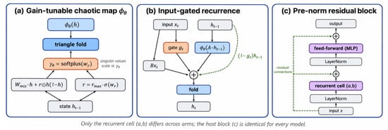
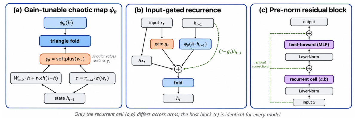
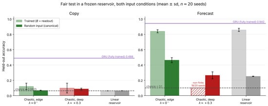
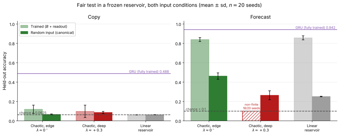
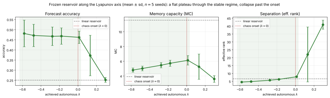
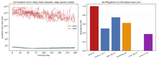
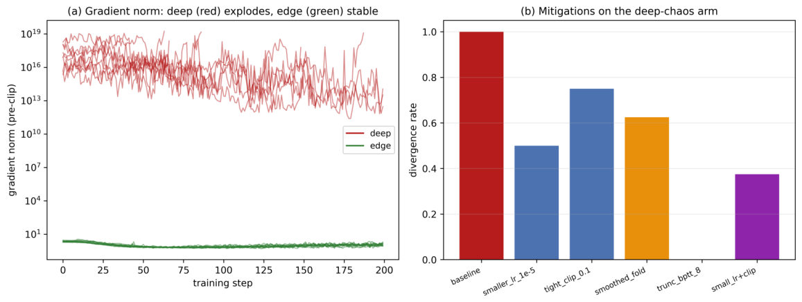
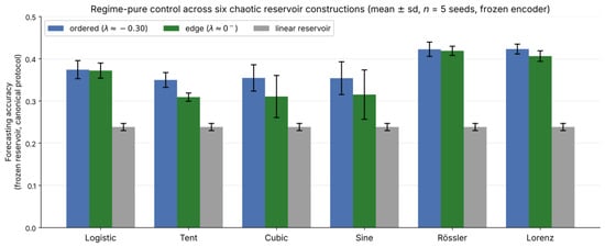
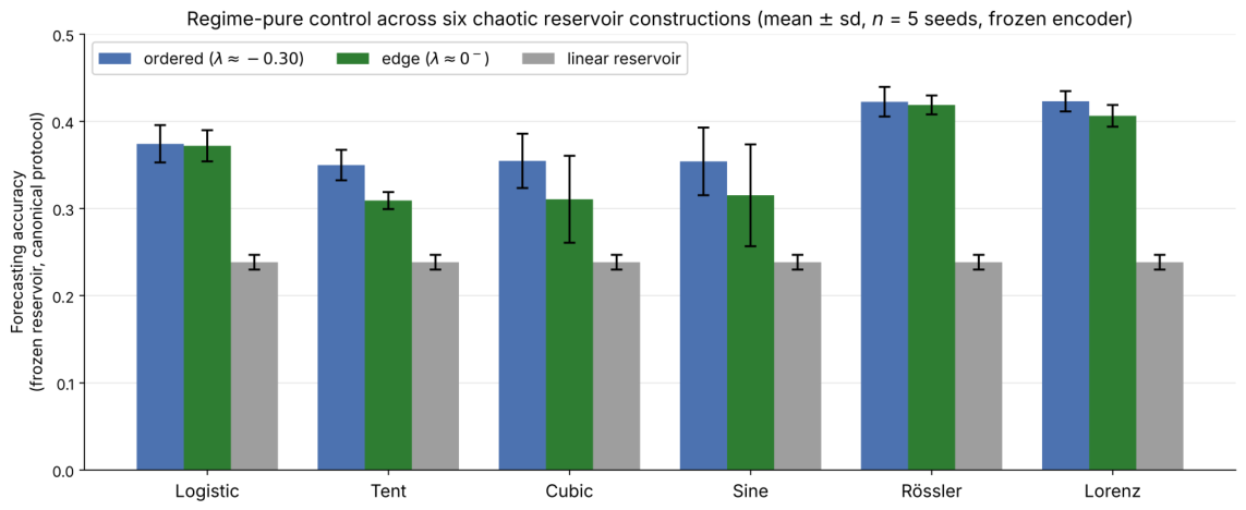
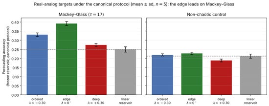
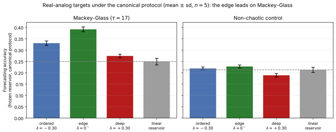
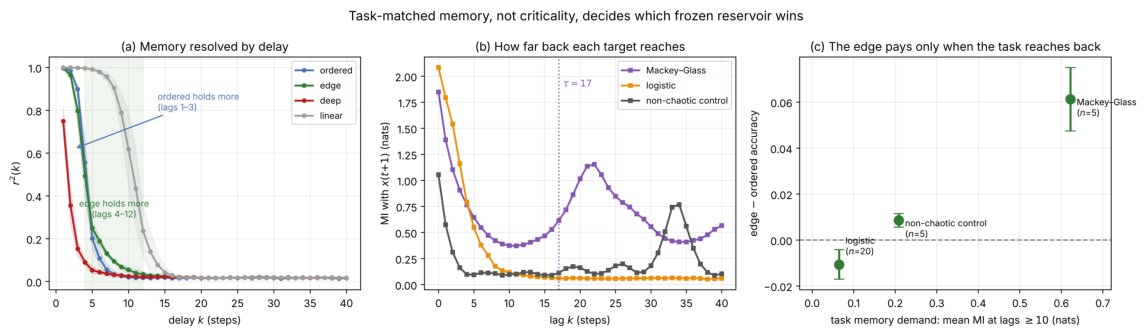
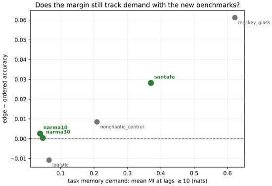
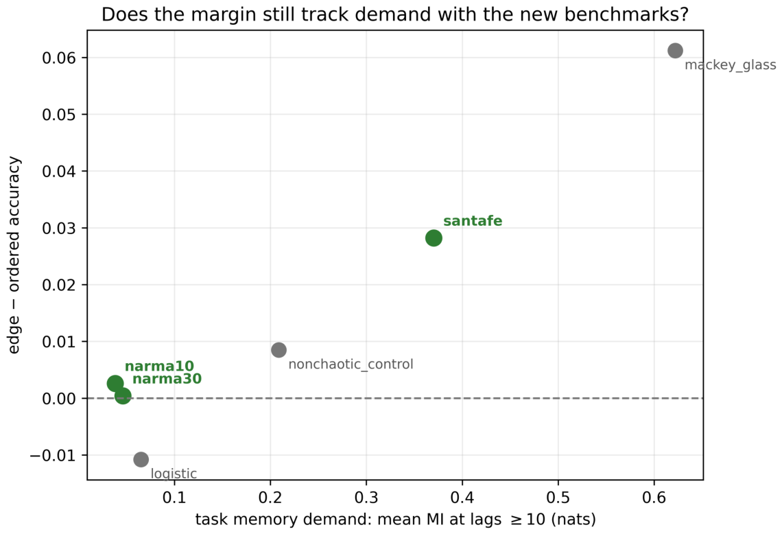
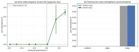
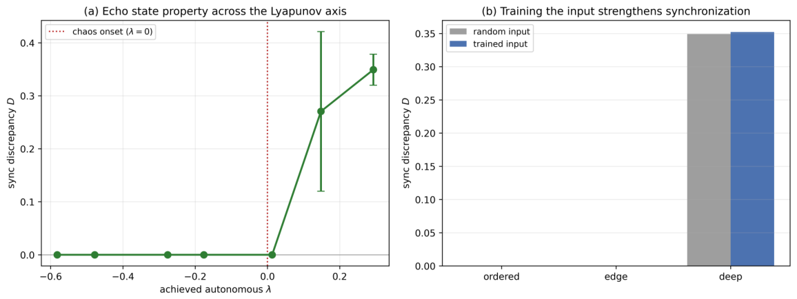
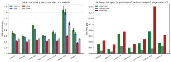
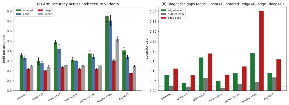
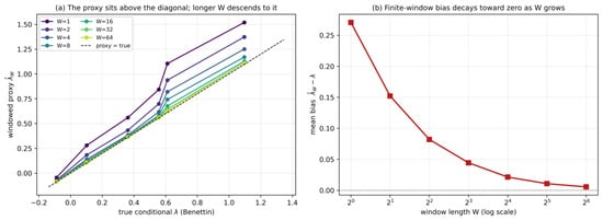
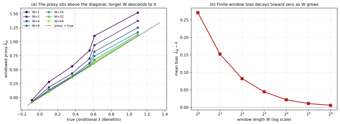
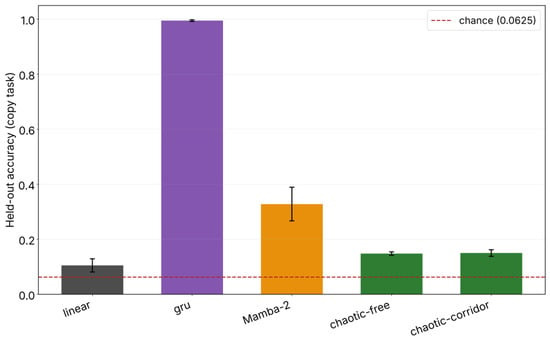
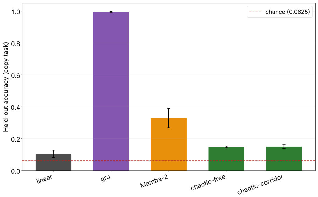
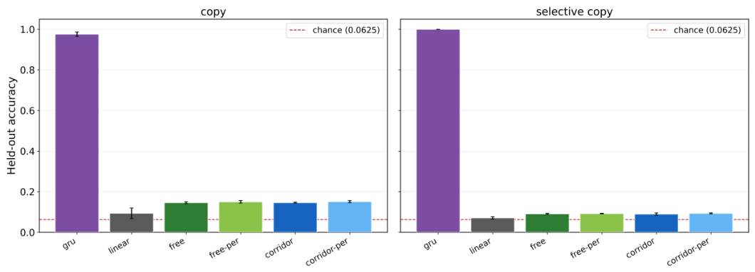
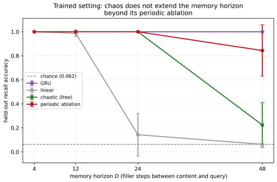
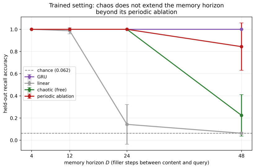
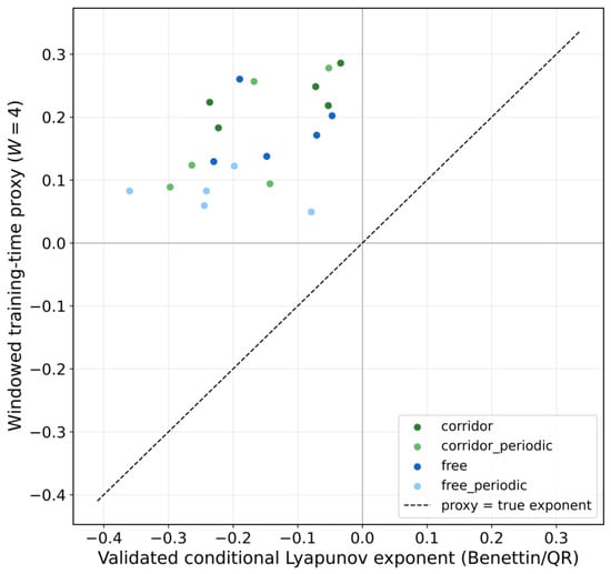
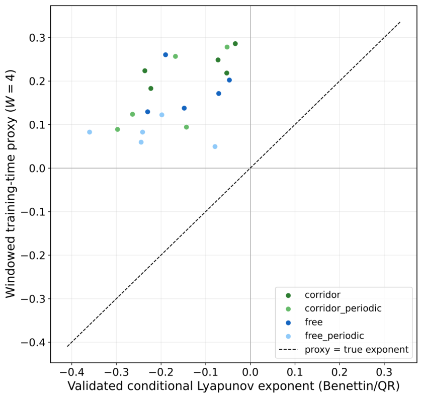
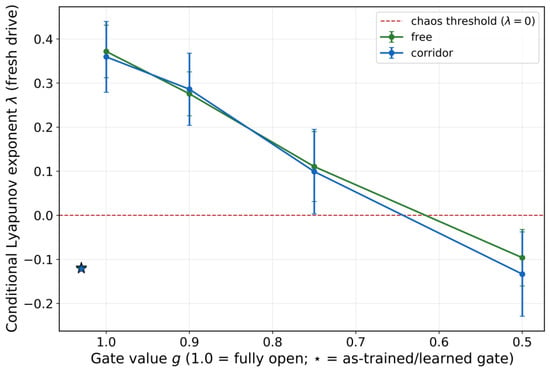
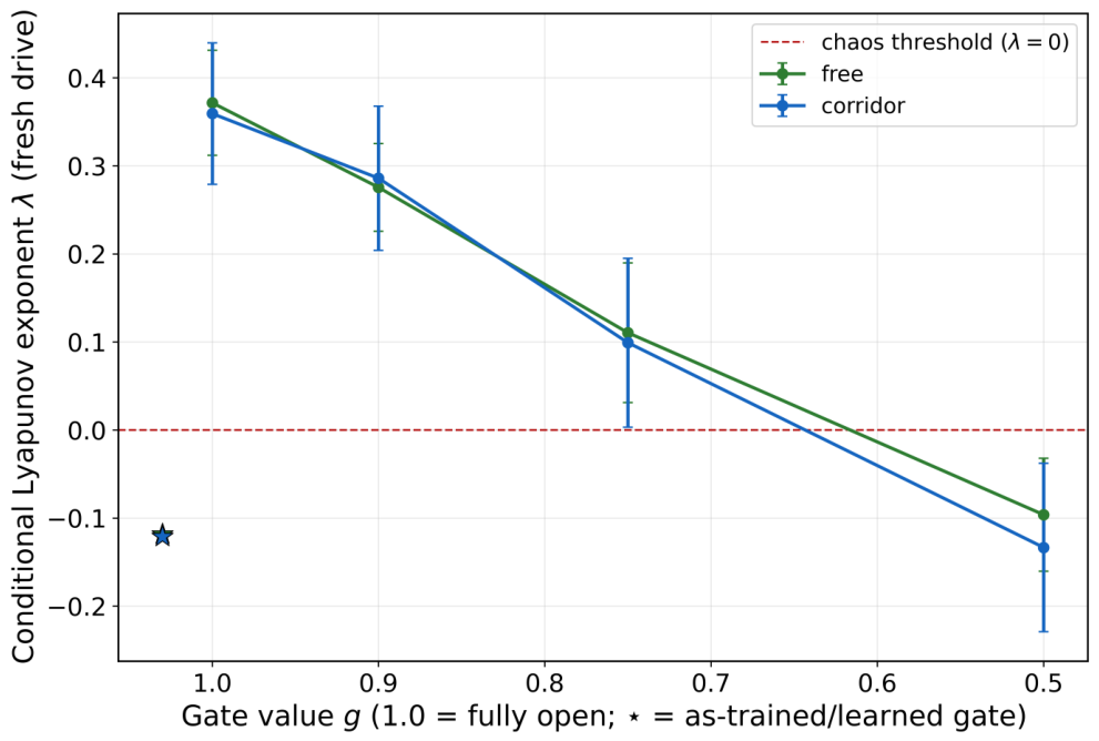

Disclaimer/Publisher’s Note: The statements, opinions and data contained in all publications are solely those of the individual author(s) and contributor(s) and not of MDPI and/or the editor(s). MDPI and/or the editor(s) disclaim responsibility for any injury to people or property resulting from any ideas, methods, instructions or products referred to in the content. |
© 2026 by the authors. Licensee MDPI, Basel, Switzerland. This article is an open access article distributed under the terms and conditions of the Creative Commons Attribution (CC BY) license.