


Abstract
We examined whether additional questionnaire items improve prediction of self-reported artificial intelligence (AI)-enabled consumer service use. Models were developed with 1565 Korean panel respondents who hesitated to shop online because their activity might be recorded. They were evaluated on 1520 such respondents one wave later. Item sets were selected under limits of 0–30 additional items, with or without prior use. All four original models using every candidate item had higher log loss (prediction error; lower is better) than their benchmarks: for ridge regression with prior use, 0.69961 versus 0.66062 for a benchmark based on prior use alone. Three models remained worse after adjustment for multiple comparisons, and no original budget policy established improvement. A single expected-benefit item gave favorable estimates, but its added value remained uncertain. Collapsing regional categories and retuning made demographic estimates slightly favorable; stronger regularization was associated with smaller excess losses, and random forests had favorable estimates. The full panel also included respondents outside the hesitation-defined group. Gains in that broader panel remained uncertain among people absent from model development. These findings concern particular fitted specifications. How information is encoded and regularized may matter as much as whether it is collected.
1. Introduction
Artificial intelligence (AI)-enabled consumer services, including shopping assistance and recommendations, create opportunities to tailor support to consumers. They also raise a practical question: which customer information is worth requesting for a prediction task? Disclosure depends on how information is requested and on its perceived use. Research on conversational interfaces and privacy policies illustrates the role of collection practices in the service experience [1,2]. We evaluate whether additional survey items improve prediction in a defined setting.
This study examines information collection in a panel-survey setting. We predict whether respondents subsequently report using a broad category of AI-enabled consumer services. We compare portfolios of demographics, expected benefits, privacy-related evaluations, consent responses, generative AI experience, and digital competence. The questionnaire item budget sets the maximum number of additional original items that may be collected for a portfolio. This distinction matters because an index supplied to a model as one variable can require eleven answers from a respondent.
Two comparisons organize the analysis. Performance preservation asks whether a smaller portfolio has acceptably similar loss to a model using every candidate block. Incremental predictive value asks whether the portfolio improves on information already available. The second comparison is especially important if the full-information model itself predicts poorly. In that setting, preservation describes performance relative to the degraded reference, while a predictive rationale for additional collection requires improvement over the existing-information benchmark. We therefore report evidence of deterioration, uncertainty about improvement, and demonstrable reductions in loss separately.
We use the 2023–2025 Panel Survey of Intelligent Information Society Users provided by the Korea Information Society Development Institute (KISDI). The original population comprises respondents who report hesitating to purchase online because their activity may be recorded. The eligibility item directly connects purchase hesitation to information collection, making this a relevant population in which to assess the predictive return from additional questions. We compare this restricted cohort with the full linked panel and evaluate common trained models across hesitation groups. The outcome records respondents’ recalled use during the preceding year.
The study addresses three questions. RQ1: Which information portfolios are selected under different item budgets and existing-information assumptions? RQ2: How do selection uncertainty, within-period validation, and later-period performance alter the assessment of these portfolios? RQ3: Which portfolios improve, preserve, or worsen predictive performance relative to explicit benchmarks, and how do those conclusions depend on the population, model, and inference procedure?
Our contribution is an empirical application of established prediction and feature-acquisition methods to a documented collection decision. The analysis connects original-item costs, an existing-information benchmark, later-period validation, and uncertainty from repeated selection. It also shows how conclusions vary with the target population and model specification. These comparisons provide evidence for reviewing questionnaire collection choices.
2. Related Literature and Analytical Perspective
2.1. Privacy, Consumer Trust, and Predictive Relevance
Privacy calculus examines disclosure decisions in relation to perceived benefits and risks, while the antecedents–privacy concerns–outcomes (APCO) framework organizes personal and contextual influences on privacy-related responses [3,4]. Awad and Krishnan associate a stronger preference for information transparency with lower willingness to accept online profiling for personalization [5]. Martin et al. show that transparency and control over firms’ data practices can alleviate the adverse effects of data vulnerability on customers and firms [6]. These perspectives motivate the study’s benefit, information-management, protection-expectation, and consent blocks.
Bleier et al. place data-based marketing within a contextual-integrity perspective: consumer concerns depend on information flows and their use [7]. This perspective motivates evaluating collection in a specified service and consumer group alongside the predictive gains that additional information provides.
Recent e-commerce research examines privacy concerns and online-shopping self-efficacy within an extended APCO model [8]. Longitudinal privacy research also distinguishes associations between people from changes within the same person [9]. This distinction matters for our eligibility rule: membership in the privacy-hesitant population can change across waves, altering the distributions and predictive relationships available to a model.
Yin et al. examine experiential benefits, perceived privacy infringement, and clicking intentions for AI-personalized recommendations [10]. Together with the privacy-calculus and APCO perspectives [3,4], this research motivates considering benefit and privacy-related information when defining candidate blocks. We assess the incremental predictive value of these blocks against existing-information benchmarks.
The present study distinguishes privacy-related purchase hesitation, which defines cohort eligibility, from annual self-reported AI-enabled consumer service use, which is the prediction outcome. This outcome covers a broader service category and recall period than a specific clicking or disclosure decision.
Trust research distinguishes cognitive evaluations from emotional responses and shows that transparency and experienced reliability operate differently across AI contexts [11]. Explainability can influence trust and acceptance [12]. Global predictive attribution instead allocates a model’s performance across inputs under a specified value function [13]. We use block attribution to describe contributions to held-out prediction loss and keep prediction quality and collection volume separate. This complements the substantive perspectives on disclosure [3,4], trust [11], and continued use [14].
The distinction between explanation and prediction is established in statistics and information-systems research [15,16]. Here, theoretical relevance defines a defensible candidate set, while incremental value is assessed against a benchmark that reflects available information. An association with service use can add little predictive value when prior use already captures the same signal. Conversely, a weak theoretical indicator can still reduce predictive error in a particular population.
2.2. Questionnaire Item Budgets, Acquisition Costs, and Data Minimization
Research on data minimization evaluates how much information can be removed while preserving a defined level of utility. Examples include limiting the ratings used for personalization [17] and generalizing feature values before collecting data for model training and deployment [18]. Scaling-law approaches examine when additional collection produces diminishing returns, while cost-restricted feature selection explicitly incorporates acquisition costs [19,20]. Marketing research likewise treats privacy and analytical utility as distinct quantities to be assessed together [21].
Saar-Tsechansky et al. connect information acquisition to expected improvement in a predictive model, treating the choice of which feature values to obtain as an economic decision [22]. Our study applies this acquisition perspective to a simpler survey design: candidate blocks are evaluated for a defined population, and cost is counted in original questionnaire items.
Our acquisition-cost unit is one original questionnaire item. It provides a reproducible way to compare a one-item benefit measure with an eleven-item competence index. Research shows that collecting less data does not automatically improve privacy or fairness [23,24]. Survey research distinguishes objective burden from perceived burden and finds that higher perceived burden accompanies poorer response quality [25]. A questionnaire-length experiment found a small increase in response rates after shortening the survey, with broadly similar sample composition and data quality [26]. These findings motivate distinguishing the number of collected items from their burden and consequences.
Existing information changes the relevant acquisition problem. We examine prior use history as available information and additionally treat demographics as already available. A zero-cost input can still worsen predictions. The selection procedure therefore evaluates whether to use each available block, with a separate sensitivity analysis requiring history and demographics to remain in every portfolio. These scenarios make the collection assumptions explicit for different organizational information settings.
2.3. Selection Stability, Temporal Evaluation, and Accountability
Model selection can overfit a validation criterion, motivating nested assessment of the complete selection process [27]. Structured data also require validation designs that reflect dependence and the intended prediction setting [28]. Feature-selection stability describes sensitivity to changes in the training sample and algorithmic randomness [29]. We report how often the original portfolio is reselected, assess its later-period performance, and repeat selection and fitting at focal budgets to quantify uncertainty. Selection recurrence is an uncorrected frequency, distinct from the chance-corrected stability estimator of Nogueira et al. [29].
Prediction loss can change when input distributions, predictor–outcome relationships, or measurement change. Concept-drift research provides a vocabulary for distributional change [30]. The 2025 questionnaire altered the outcome instruction and added explanatory material. Our instrument audit, paired responses, and recalibration diagnostics examine the resulting changes in reported use and prediction.
Responsible AI auditing emphasizes documentation throughout the system lifecycle [31]. The National Institute of Standards and Technology (NIST) AI Risk Management Framework connects governance with identifying, measuring, and managing AI risks [32]. For collection review, this record should connect an item’s purpose, representation, and cost to its predictive contribution and later performance. Our analysis provides an example of this evidence.
3. Materials and Methods
3.1. Data, Eligibility, and Temporal Design
We used the numeric microdata, questionnaires, and codebooks for KISDI survey waves conducted in 2023, 2024, and 2025 [33,34,35]. Annual files contained 4581, 4420, and 4324 respondents, respectively. Identifiers were used only to link observations and define participant overlap. The development transition used baseline 2023 predictors and the 2024 outcome; temporal evaluation used baseline 2024 predictors and the 2025 outcome. Baseline purchase-hesitation responses coded “always” or “sometimes” defined the original restricted population. The resulting samples contained 1565 and 1520 respondents. The full linked-panel sensitivity included respondents across all hesitation categories, with 3895 and 3741 respondents with the defined outcome. The restriction retained 40.2% and 40.6% of the linked samples, respectively, reducing sample size and potentially limiting precision for detecting small incremental gains. Figure 1 summarizes the analysis workflow.
Figure 1.
Study design and analysis workflow. The original cohorts are reconstructed from the 2023–2025 KISDI panel. Models are selected using development data and scored in the later period. At budgets 1 and 4, bootstrap repetitions resample participants across both periods and repeat model development. Additional analyses examine calibration, population differences, wider model searches, regional coding, and adjacent-service responses. The later period was examined in the original analysis. HGB = histogram-based gradient boosting; P0 = history-based benchmark; NONE = overall-rate benchmark. CV = cross-validation. Arrows show the wave transitions and the sequence of analysis steps. Blue boxes show development and model selection, peach boxes show temporal evaluation, and gray boxes show the survey, comparisons, and follow-up checks. H = prior use history. D = demographics.
There are 641 participants in both restricted samples, representing 42.2% of the 1520 evaluation respondents. We call the remaining 879 respondents the person-disjoint subset, meaning that they were absent from the corresponding development sample. This subset includes 728 people observed in 2023 who did not meet the earlier hesitation rule and 151 people absent from the 2023 file. In the full linked panel, 3333 of 3741 evaluation respondents overlap with its development sample (89.1%), leaving a person-disjoint subset of 408. Thus, overlap is defined relative to the development population used to train each model. Supplementary Section S1 documents linkage and composition.
This study is a retrospective, exploratory secondary analysis. The later-period outcomes were examined in the original analysis. All tuning and portfolio selection used development data; additional analyses reused the observed evaluation period. The original comparison families remain the primary comparisons, with exploratory and post hoc analyses reported separately (Section 5.1). The estimands concern prediction of self-reported use, not causal privacy effects, logged behavior, or the effect of a collection policy on consumer welfare.
3.2. Outcome, Information Blocks, and Measurement Audit
The outcome is reported use during the preceding year of intelligent services in the consumption domain, termed AI-enabled consumer services here. Codes 1–4 indicate any use; codes 5 and 9 indicate no use. Code 9 means never used and is retained as a valid response. Prior use history H is the same binary measure in the baseline year. Self-reported digital behavior can differ from recorded behavior [36].
Table 1 defines the eight information blocks. The seven optional blocks require 30 original items. Protection expectations P and digital competence K each entered the model as one eleven-item mean, calculated when at least eight and nine items, respectively, were valid. These content-based indices summarize their constituent responses. All items needed for these indices were observed in the annual source data. Expected benefits B and information management M treated “do not know” as missing. In the restricted development/evaluation samples, B had 53/52 missing values, and M had 0/7. Numeric imputation and scaling, and categorical imputation and one-hot encoding, were fitted within each training partition for the original models; the CatBoost sensitivity used the categorical handling described in Section 3.6. Supplementary Section S2 provides source-variable names, permissible codes, item correspondence, and preprocessing.
Table 1.
Information blocks and original-item acquisition counts.
For generative-AI experience A, code 1 indicates prior experience, and code 2 indicates no experience. We summarized its prevalence and the next-year outcome rate within each response category in both restricted samples. Unadjusted odds ratios with pointwise 95% log-Wald intervals summarized the association in each period. These descriptive diagnostics and the cross-wave item audit appear in Supplementary Section S12.1 and Table S36.
The questionnaires retained the consumption-domain row label, past-year recall period, and response-code scheme across waves. The 2025 Q1 instruction added the Korean word for “frequently,” and later pages expanded explanations of consumption, leisure, and work services. Leisure examples also changed between 2023 and 2024, while work examples changed between 2024 and 2025. The neighboring domains served as comparison outcomes with documented wording changes. We assessed paired response changes using participant resampling and exact McNemar tests [37]. Additional three-wave comparisons examined whether consumption changes differed from leisure and work. Logistic response models adjusted for observed neighboring-domain response patterns, using participant-cluster sandwich covariance corresponding to the generalized estimating equations (GEE) approach with an independent working correlation [38] (Supplementary Section S11). Logistic-regression differential item functioning (DIF) procedures compare item responses across groups conditional on a matching measure of the construct [39]. In this study, the models estimated conditional response change using neighboring-domain patterns as observed covariates. The diagnostics therefore assessed differences in reported change under the documented instrument conditions. Section 5.4 addresses the measurement evidence needed to interpret these patterns.
Table 2 summarizes the reconstructed sample sizes and event counts.
Table 2.
Reconstructed analytical samples.
3.3. Item Budgets, Benchmarks, and Model Selection
For portfolio S, collection volume is the sum of original item counts for included optional blocks: D = 4, B = 1, M = 1, P = 11, C = 1, A = 1, and K = 11. H was assigned zero additional cost when available; the history-unavailable condition used the seven optional blocks. The budget b ranged from 0 to 30 and set the maximum number of additional items; eligible portfolios could use fewer items. This incremental budget counted optional-block items beyond the screening and outcome questions common to all portfolios.
The no-additional-collection benchmark P0 predicts a Laplace-smoothed development outcome rate separately for H = 0 and H = 1. NONE predicts the smoothed overall development outcome rate. For a group with n observations and y events, the prediction is (y + 1)/(n + 2). P0 uses these smoothed rates directly; ridge and gradient-boosting models using H alone estimate their predictions through model fitting and tuning. When history was available, selection considered all 256 subsets of eight blocks, including subsets omitting H, plus P0. When history was unavailable, selection considered the 128 subsets of the seven optional blocks; the empty subset was NONE.
The original model families were ridge logistic regression and histogram-based gradient boosting (HGB), implemented in scikit-learn 1.8.0 [40]. Ridge considered inverse penalty values 0.001, 0.01, 0.1, 1, and 10. HGB considered three or seven leaves, with 100 iterations, learning rate 0.05, minimum leaf size 20, L2 penalty 1, and early stopping disabled. Five-fold stratified out-of-fold log loss determined hyperparameters and the lowest-loss eligible portfolio at each budget. Ties favored fewer additional items and then lexical portfolio order. We fitted the chosen configuration on the complete development sample for temporal evaluation. The full-information reference included all seven optional blocks, plus H when available. Selection at budget 30 followed the development-loss criterion and could yield a portfolio with fewer blocks.
The original repeated nested cross-validation used two repetitions of five outer folds, with five-fold tuning and portfolio selection inside each outer training set. Its stored results provided development diagnostics. The raw-data reconstruction refitted every frozen temporal model, while retaining the complete nested-analysis results. Because the ten outer training sets overlap, recurrence across them describes selection within overlapping samples. Repeated holdouts and the full-process bootstrap further assessed selection variability.
3.4. Prediction Loss, Comparison Families, and Precision
Log loss is the mean negative logarithm of the probability assigned to the observed binary outcome, a strictly proper scoring rule [41]. Lower values are better. For each observation, we subtracted the reference loss from the candidate loss and averaged these paired differences. Throughout, Δ denotes candidate log loss minus reference log loss: positive values indicate deterioration, and negative values indicate improvement. We report absolute losses alongside contrasts, the area under the receiver operating characteristic curve (ROC AUC) with confidence intervals, Brier scores, average precision, and calibration diagnostics.
For each original algorithm, history condition, and evaluation group, the primary simultaneous family included every distinct nonzero contrast of the 31 selected budgets against both the full-information model and P0 or NONE. Each distinct contrast appeared once. This gave 21, 25, 31, and 28 contrasts for ridge without H, ridge with H, HGB without H, and HGB with H, respectively. Including every budget protected inference across the displayed frontier but reduced precision for focal low-budget decisions. Section 5.1 summarizes these primary families and the additional analyses.
We used a single-step joint confidence region based on the maximum centered, unstudentized paired-bootstrap error over the family [42]. With 5000 evaluation-participant resamples, let e be a bootstrap contrast minus its observed contrast. The 95th percentile of the maximum negative e gives the upper-bound increment; the 95th percentile of the maximum e gives the lower-bound decrement. Two-sided 95% intervals used the 95th percentile of the maximum absolute e. Identity contrasts remained zero. These bounds are conditional on fitted predictions. The original 2000-repetition upper bounds (seed 20260909) were independently reproduced. The primary simultaneous comparison families used 5000 repetitions and seed 20261020. Other contrast families used analysis-specific seeds documented in the Supplementary Materials and the public analysis scripts identified in Supplementary Table S26. Figure 2 used seed 2026102002 for pointwise percentile intervals around absolute log loss.
Figure 2.
Development and temporal performance across item budgets. The orange development curve averages two retained nested cross-validation repetitions; its orange shaded range spans their means and is descriptive. The blue line shows temporal evaluation. Its blue bands are pointwise 95% participant-bootstrap intervals for absolute log loss, with predictions fixed (5000 draws; seed 2026102002). This differs from seed 20261020 used for the primary simultaneous comparison families in Section 3.4. Lower log loss is better. H denotes prior use history. The dashed line shows the temporal benchmark. The four panels share the same axis scales. P0 is the history-based benchmark; NONE is the overall-rate benchmark; HGB is histogram-based gradient boosting. Aggregate data for all 31 budgets are identified in the Data Availability Statement.
Improvement requires a one-sided simultaneous upper bound below zero; deterioration requires a lower bound above zero. Non-inferiority to a specified reference requires the upper bound to fall below an allowable increase δ. We used 0.0025, 0.005, and 0.01 as numerical sensitivity margins and reported δ = 0 separately as the superiority boundary. Non-inferiority at positive δ can coexist with evidence of deterioration, so the two judgments are recorded separately. Establishing collection benefit requires a favorable comparison with P0 or NONE, alongside any preservation relative to the full model.
We additionally examined benchmark-only families, budgets 0–4, and bounds standardized by a fixed bootstrap standard error for each contrast. The standard error was held constant across resamples, which distinguishes this scaling from a bootstrap-t procedure. These exploratory sensitivity analyses supplemented the original comparison family. The direct comparison of the four original full models with their respective benchmarks used a separate four-contrast family within each evaluation group. Approximate 80% minimum detectable effects combined the observed paired-loss standard error with a one-sided critical value and the 80th percentile of a standard normal distribution. These quantities summarize conditional precision under the stated normal approximation. Supplementary Section S4 gives formulas and complete family-specific results.
3.5. Repeating Selection and Diagnosing Temporal Differences
We completed 1000 bootstrap repetitions of model development at budgets 1 and 4. In each repetition, we resampled the 2444 distinct participants in the restricted samples. A participant present in both periods received the same multiplicity in each, and all copies remained together in an inner fold. We repeated preprocessing, five-fold tuning, portfolio selection, and final fitting across the 34 eligible original portfolios plus P0. Full-information references were retuned and fitted separately. Pointwise percentile intervals summarized the complete procedure. Supplementary Section S5 and Table S12 compare percentile and basic intervals, bootstrap bias, and convergence [43]. With 1000 repetitions, approximately 25 draws fall in each 2.5% tail, and the worst-case Monte Carlo standard error of a selection frequency is 1.58 percentage points. Supplementary Table S27 details the inferential scope.
We also repeated twenty stratified 70/30 splits of the development sample, using 1095 training and 470 holdout observations. We repeated inner five-fold selection within training and evaluated the same fitted models on both the within-period holdout and the later cohort. This held training size constant when comparing periods. Quantiles over overlapping splits provide descriptive summaries of split variability.
For calibration diagnostics, we fitted intercept-only or intercept-and-slope logistic recalibration to evaluation predictions. We reported apparent and five-fold cross-fitted recalibration separately. Empirical outcome entropy is the loss of a constant predictor equal to the evaluation event proportion. Affine resolution equals entropy minus apparent affine-recalibrated loss; affine miscalibration equals raw loss minus apparent affine-recalibrated loss. Hence, raw loss equals entropy minus resolution plus miscalibration. The constant-prevalence reference differs from intercept-only recalibration of the original score. The decomposition applies to affine recalibration. To obtain intervals, we refitted the recalibrator in 500 bootstrap resamples while holding base predictions fixed. These retrospective diagnostics used evaluation outcomes.
3.6. Expanded Models, Population Sensitivity, and Block Attribution
Additional analyses compared development-tuned ridge, HGB, random forests [44], and extra trees [45] in both restricted and full linked-panel samples. Ridge used 13 inverse-penalty values from 10−4 to 102. HGB used 24 combinations of learning rates 0.03, 0.05, and 0.1; 100 or 300 iterations; and 3, 7, 15, or 31 leaves. Each tree-ensemble family used six configurations with 200 trees. We evaluated eight fixed information representations in this exploratory comparison, fitting 64 models, evaluating 784 configurations, and completing 3920 inner-fold fits. This comparison assessed robustness across the specified models, representations, and search grids.
A further comparison included XGBoost 3.4.1, LightGBM 4.7.0, and CatBoost 1.2.10 [46,47,48]. Each used twelve configurations across the same eight representations and two populations, giving 48 final models and 2880 development-fold fits. Tuning minimized pooled five-fold development loss using the same folds as the expanded comparison. XGBoost and LightGBM used imputation, scaling, and one-hot encoding fitted within each training fold. CatBoost used imputed categorical strings and ordered boosting. These learners were evaluated at the eight specified representations; exhaustive budget selection was performed for the original ridge and HGB models. The added full-model comparisons formed a separate six-contrast family within each population and evaluation group. Supplementary Section S7 gives the grids and results.
Within each population and evaluation group, 5000 paired bootstrap resamples provided simultaneous two-sided intervals across eight full-model contrasts: four algorithms with and without H. Original-model AUC intervals used 2000 participant-bootstrap resamples; expanded-model AUC intervals used DeLong placement variances [49] and normal limits. Both are conditional on fitted models. We evaluated the same models trained on the full panel among hesitant respondents and other linked respondents, further separating rare-or-never hesitation from no relevant experience. These comparisons describe predictive differences between observed groups. Supplementary Table S37 reports development-participant overlap within each group.
A regional-encoding analysis compared the original 17 categories with a capital-region indicator: Seoul, Incheon, and Gyeonggi versus all other regions. The mapping was fixed geographically, and both encodings underwent the same development-only five-fold tuning for demographic and full-information representations under the original Ridge/HGB grids. D retained its four-item cost. Within each evaluation group, separate simultaneous families covered eight paired encoding differences and sixteen original/coarsened model-versus-benchmark contrasts. This retrospective diagnostic evaluated encoding and retuning together, retaining all demographic variables in the specified representations.
The existing-H + D scenario assigned both blocks zero incremental cost, leaving at most 26 new items. We compared optional use with required inclusion of H and D, using the development-selected zero-cost model, fixed H + D, and P0 as references. Longitudinal-weight sensitivity compared weighted and unweighted losses on the same 1369 respondents with valid weights. This analysis described prediction scores under alternative weighting of these respondents.
Exact Shapley allocation averages each optional block’s held-out loss reduction over all subsets of the other six blocks [13,50]. For attribution, H was fixed as present or absent; when H was available, budget selection considered portfolios with and without it. Positive allocation means improved prediction. We reported total allocation and allocation per original item. The per-item ratio was calculated after the original Shapley allocation by dividing each block’s allocation by its item count. It describes predictive efficiency within that game. Simultaneous intervals covered 56 block, algorithm, history, and evaluation-group combinations with fitted predictions held fixed. Supplementary Materials give the sensitivity analyses, alternative outcome codings, and execution records.
3.7. Reproducibility and AI Assistance
The reanalysis read the original workbooks from 2023 to 2025 and checked them against the instruments and codebooks. It reproduced all 512 frozen ridge/HGB temporal log-loss values exactly and the original simultaneous upper bounds to a maximum absolute difference of 1.1 × 10⁻¹⁵. Source hashes, seeds, configuration grids, software versions, code, and aggregate outputs are identified in the Data Availability Statement and Supplementary Section S10. Scikit-learn 1.8.0 was used for model fitting [40]. We regenerated the initial 200 bootstrap repetitions using the same archived fitting code and documented software versions as the remaining 800. All replicate-level results and reported summaries were identical (Supplementary Section S5). The bootstrap verification used Python 3.12.14, NumPy 2.3.5, pandas 2.2.3, SciPy 1.17.0, joblib 1.5.3, and threadpoolctl 3.6.0. The archived requirements specify openpyxl 3.1.5 for reading workbooks and Matplotlib 3.10.8 for plotting.
ChatGPT (OpenAI, San Francisco, CA, USA; 5.6 Sol in the initial preparation record) and ChatGPT Work Mode supported English translation; manuscript organization and language editing; analytical and plotting code; and numerical, citation, and narrative consistency checks. OpenAI Codex in ChatGPT Work Mode assisted with formatting, figure typography, and document checks in the present revision. The authors checked AI-assisted suggestions against the instruments and analytical evidence and retain responsibility for verification, scientific interpretation, and the final content. The service websites are https://chatgpt.com/ for ChatGPT and https://openai.com/codex/ for Codex (both accessed on 8 November 2026).
4. Results
4.1. Sample Composition and Measurement Checks
The restricted development and evaluation event proportions were similar, at 56.23% and 56.12%. Among the 641 shared participants, however, any reported use decreased from 66.61% to 59.59%, a change of −7.02 percentage points (paired 95% interval −11.54 to −2.65). Monthly use decreased from 57.10% to 41.81%, or −15.29 points (−19.97 to −10.45). Both changes remained detectable after adjustment across the three outcome thresholds.
Three-wave adjacent-domain comparisons describe the specificity of these changes (Supplementary Tables S33–S35). Among the same 641 participants, the 2024–2025 change in consumer-service use was 9.05 percentage points below the leisure change (simultaneous 95% interval −16.39 to −1.71) and 12.64 points below the work change (−20.42 to −4.85). The corresponding changes in these differentials relative to 2023–2024 were −12.32 points (−25.52 to +0.87) and −10.61 points (−24.43 to +3.22). A logistic model adjusting for the observed leisure/work response pattern gave a 2025-versus-2024 odds ratio of 0.587 (pointwise 95% interval 0.465–0.741; Holm-adjusted p = 0.000081 [51]). Results vary across thresholds and cohorts; in the full three-wave panel, a consumer–leisure differential was already present in 2023–2024.
The shared participants and person-disjoint subset also differed. Baseline use prevalence was 66.61% and 67.58%, respectively, whereas follow-up use was 59.59% and 53.58%. Table 3 compares demographics. Embedded codebooks define identical sex, age, education, and region categories across all three waves. The standalone codebooks omit the seventies age category, which is defined in the embedded codebooks but absent from all analytical baseline samples. Among the 641 shared participants, 82 moved to the next age group, and two changed recorded education categories between the 2023 and 2024 baselines. Recorded sex and region remained unchanged. Under ridge with H fixed, the demographic loss-reduction allocation changes from +0.01761 in development out-of-fold scores to −0.04158 in temporal evaluation. Both use the same seven-block game and a tuned H-only reference; development attribution reuses tuning folds and is descriptive.
Table 3.
Baseline demographic distributions and coding audit (%).
The apparently stable capital-region share (44.4% in development and 45.0% in evaluation) masks changes within that region: Seoul rises from 17.0% to 26.9%, Incheon falls from 5.9% to 1.7%, and Gyeonggi falls from 21.5% to 16.4%. Table 3 displays these components separately. The encoding analysis in Section 4.4 examines whether retaining all 17 regional categories contributes to the performance pattern.
4.2. Original Full Models and Selected Collection Budgets
Table 4 places the original full-information models beside their benchmarks. All four full-model estimates are worse. With H available, ridge and HGB losses are 0.69961 and 0.67063, compared with 0.66062 for P0. Without H, their losses are 0.70911 and 0.71281, compared with 0.68564 for NONE. A simultaneous comparison across these four contrasts supports deterioration for ridge with and without H and HGB without H; the interval for HGB with H included zero.
Table 4.
Original full-information models versus no-additional-collection benchmarks.
At budget 1, all original conditions select B, with H included when available. At budget 4, all select D, again with H when available. Larger-budget selections can use fewer items than permitted: ridge selections at budget 30 use 29 items with H and 28 without H, compared with 30 optional items in the full-information references. Figure 2 compares the retained nested development results with temporal performance across the entire frontier. Supplementary Section S3 reports the portfolios. The repository identified in the Data Availability Statement provides the aggregate source data for Figure 2.
The one-item selections have favorable loss differences against their benchmarks, ranging from −0.00820 to −0.00338, but every original-family upper bound remains above zero (Table 5). Relative to their respective benchmark losses, these point-estimated reductions are 0.51–1.20%; they describe the magnitude of the observed prediction differences. Three have negative upper bounds against their full-information reference; HGB H + B has an upper bound of +0.00667 and meets preservation only at a sufficiently permissive margin, including 0.01. None of the one-item policies meet non-inferiority against P0 or NONE at margins up to 0.01 under the primary unstudentized family. These comparisons show that performance preservation and benchmark-relative value depend on the chosen reference.
Table 5.
Focal original selections and separate one-sided simultaneous bounds against benchmarks.
The four-item ridge H + D selection has Δ = +0.03571 against P0, with a one-sided simultaneous lower bound of +0.01369. Ridge D and HGB D have lower bounds of +0.00236 and +0.00727 against NONE. Thus, deterioration is supported for these three frozen fitted portfolios. The HGB H + D lower bound is −0.00186, leaving deterioration uncertain at the same familywise level. Figure 3 reports two-sided simultaneous intervals, unlike the separate one-sided bounds in Table 5.
Figure 3.
Temporal loss differences of focal original selections. A positive difference in log loss indicates higher loss than P0 (H available) or NONE (H unavailable). Bars are two-sided simultaneous 95% bootstrap intervals based on the maximum absolute centered error, separately within each original algorithm × history-availability family containing all selected budgets and both references; 5000 paired evaluation resamples, n = 1520. The eight displayed contrasts retain their original family memberships. Predictions are fixed. P0 = history-based benchmark; NONE = overall-rate benchmark; HGB = histogram-based gradient boosting. H = prior use history. B = expected benefit of consumer AI services. D = demographics. The dashed vertical line marks zero difference from the benchmark.
Across the full original frontier, simultaneous lower bounds support deterioration at 26 of 31 budgets for ridge with H, 11 for ridge without H, 22 for HGB with H, and 26 for HGB without H. The corresponding counts in the person-disjoint subset are 27, 27, 25, and 27. None of the 248 budget, condition, and evaluation-group entries establishes improvement under its primary family. These are policy rows, including repeated portfolios, rather than 248 independent tests. Supplementary Tables S4–S7 report both bounds; Supplementary Table S29 summarizes the two evaluation groups.
The one-item inference is sensitive to adjustment. For ridge B without H, the pointwise upper bound is −0.00284, the original-family unstudentized upper bound is +0.01459, and the standardized bound for the original family is +0.00015. Standardized benchmark-only families give upper bounds of −0.00109 across all budgets and −0.00145 across budgets 0–4. Approximate 80% detectable magnitudes for the four one-item contrasts are 0.00607–0.00946 pointwise and 0.02300–0.02557 under the primary families, compared with observed improvements of 0.00338–0.00820. Supplementary Table S11 gives the precision calculations.
4.3. Selection Uncertainty, Within-Period Performance, and Calibration
Across 1000 repetitions of model development, the original one-item portfolio was selected in 65.6–84.3% of repetitions. At budget 4, demographic portfolios recurred in 92.6% of ridge repetitions with H, 80.8% of ridge repetitions without H, 79.9% of HGB repetitions with H, and 59.5% of HGB repetitions without H.
All eight complete-procedure percentile intervals for loss differences against P0 or NONE include zero (Figure 4). For ridge H + D, the original Δ of +0.03571 has a pointwise 95% interval of −0.00618 to +0.07080 after repeating selection and fitting. For ridge H + B, Δ is −0.00338 with an interval of −0.00793 to +0.02974. Results vary with interval construction; Supplementary Section S5 and Table S12 give the basic-interval comparison and bootstrap bias.
Figure 4.
Selection recurrence and uncertainty after repeating model development. (Left) Blue bars show how often the original portfolio was reselected across 1000 bootstrap repetitions. (Right) Orange points show the original contrasts and horizontal orange bars show the pointwise 95% percentile intervals against P0 (history-based benchmark) or NONE (overall-rate benchmark). Shared participants received the same multiplicity in both periods, and copies remained together in inner folds. Preprocessing, tuning, selection, and fitting were repeated at budgets 1 and 4. The exploratory intervals summarize individual contrasts. HGB = histogram-based gradient boosting. Supplementary Table S12 reports sensitivity to interval construction. H denotes prior use history. The dashed vertical line marks equal model and benchmark loss.
The resampled development datasets contain, on average, 63.2% distinct participants relative to their row count. At budget 4, the original weakly regularized configuration recurs in only 12.4–24.9% of repetitions. Mean benchmark-relative losses are approximately +0.032 to +0.052 when that configuration is selected, compared with +0.004 to +0.014 under stronger regularization (Supplementary Table S30). These descriptive comparisons are conditional on the selected configuration, while the resampled participants, tuning, and portfolio selection also change.
At matched training size, the within-period and later-period results still differ. For budget-4 ridge with H, mean within-period loss is 0.64616 versus 0.66522 for P0 (Δ = −0.01906). The same fitted models give later-period loss of 0.69165 versus 0.66066 for P0 (Δ = +0.03099). For HGB, the corresponding differences are −0.01128 and +0.00726. Figure 5 presents the distributions across splits.
Figure 5.
Within-period and later-period performance at matched training size. Twenty stratified 70/30 development splits repeat five-fold tuning and budget-4 selection. Each model is applied to its 470-person holdout and the later cohort of 1520. Points are mean model-minus-benchmark loss differences; bars span the 2.5th–97.5th percentiles across overlapping splits and are descriptive. The benchmark is P0 (history-based rate) with H and NONE (overall rate) without H. HGB = histogram-based gradient boosting. H = prior use history. The dashed vertical line marks equal budget-4 model and benchmark loss.
Affine recalibration removes part of the excess loss. Ridge H + D has a raw loss of 0.69634. Its apparent affine-recalibrated loss is 0.67280, and its cross-fitted recalibrated loss is 0.67315. Its calibration slope is 0.411 (pointwise 95% interval 0.258–0.567). The cross-fitted loss still exceeds P0’s original 0.66062. For the full models with H, cross-fitted recalibration changes ridge loss from 0.69961 to 0.66889 and HGB loss from 0.67063 to 0.66332. Ridge H + B changes little, from 0.65724 to 0.65708.
Demographic-only discrimination is weak: whole-sample AUC is 0.5384 for ridge and 0.5405 for HGB. In the person-disjoint subset, their AUCs are 0.4912 (95% interval 0.4529–0.5300) and 0.4936 (0.4555–0.5335), and their calibration-slope point estimates are negative with intervals spanning zero. The diagnostics identify miscalibration together with limited ranking information in the loss pattern. Table 6 reports AUC intervals for the person-disjoint subset for the main original models, including low-budget selections and full references.
Table 6.
Temporal performance of original models in the person-disjoint subset (n = 879).
4.4. Expanded Algorithms and the Full Linked Panel
Wider searches produced no supported improvement among the fourteen restricted-cohort full-information contrasts: eight expanded-grid and six additional-boosting comparisons. Four supported deterioration under their respective simultaneous families. Random forests have favorable point estimates with H and without H (Δ = −0.00883 and −0.00968), but both intervals include zero. Expanded-grid ridge with H and HGB with and without H retain adverse intervals, as does LightGBM without H.
In the full linked panel, seven of eight expanded-family contrasts favor improvement; the interval for HGB with H included zero (Figure 6). Expanded-grid ridge with H has a loss of 0.63143 versus 0.65171 for P0, giving Δ = −0.02029 (simultaneous 95% interval −0.03423 to −0.00634). Ridge without H gives Δ = −0.04407 (−0.05802 to −0.03013). Random forests and extra trees with H give Δ = −0.01456 (−0.02850 to −0.00062) and −0.02260 (−0.03654 to −0.00866), respectively.
Figure 6.
Additional-information value varies by model and prediction population. Four algorithms use development-only expanded searches. Each panel contains a separate eight-contrast family: full with H versus P0 and full without H versus NONE, across four learners. Bars are two-sided simultaneous 95% paired-bootstrap intervals based on the maximum absolute centered error within each panel (5000 repetitions), conditional on fitted models. Development/evaluation n = 1565/1520 for the restricted population and 3895/3741 for all linked respondents. These are retrospective sensitivity comparisons. P0 = history-based benchmark; NONE = overall-rate benchmark; HGB = histogram-based gradient boosting. H = prior use history. The dashed vertical line marks equal full-model and benchmark loss.
Table 7 reports the direct XGBoost, LightGBM, and CatBoost comparison under the added six-contrast families. In the restricted cohort, LightGBM without H has higher loss than NONE (Δ = +0.03490; simultaneous 95% interval +0.01316 to +0.05664); the other five intervals include zero. In the full linked panel, XGBoost without H, LightGBM without H, and CatBoost with and without H improve on their respective benchmarks. These four loss differences range from −0.04996 to −0.02751, whereas the other two intervals include zero. These results locate the gains within particular model and population specifications; the added-learner comparison evaluates fixed representations. In the full-panel person-disjoint subset (n = 408), only one of eight expanded-family intervals and none of the six added-boosting intervals exclude zero in favor of the full-information model (Supplementary Tables S16 and S18).
Table 7.
Direct XGBoost, LightGBM, and CatBoost full-information comparisons.
Using the same ridge model with H trained on the full panel, Δ is +0.00194 among hesitant respondents and −0.03550 among other linked respondents. Across the seven expanded or additional learners and two history conditions, none of the fourteen contrasts from models trained on the full panel supports improvement in the hesitant group, whereas thirteen support improvement among the other 2221 respondents. That comparison group combines 1995 rare-or-never-hesitant respondents and 226 reporting no relevant experience. Among the former alone, eleven of fourteen contrasts support improvement. Across the four original-grid contrasts, fourteen restricted-trained wider-model contrasts, and fourteen contrasts from models trained on the full panel evaluated in the hesitant group, there are zero supported improvements and seven supported deteriorations out of 32. The counts summarize distinct analysis families rather than one joint 32-test family. Supplementary Section S7 reports the group-specific comparisons.
Relative to the full-panel development sample of 3895, 1369 of 1520 hesitant evaluation respondents overlapped (90.07%), compared with 1964 of 2221 other respondents (88.43%). The corresponding person-disjoint subsets contained 151 and 257 respondents (Supplementary Table S37). These proportions use the full-panel training population; the 641 shared participants reported above use the restricted development population.
Within the restricted evaluation cohort, three of four original full-model estimates favor improvement among the 641 shared participants; however, their simultaneous intervals include zero. All four estimates are adverse in the person-disjoint subset of 879, and three support deterioration (Supplementary Table S31). Both groups received the same 2025 instrument.
Coarsening region and retuning improve seven of eight demographic/full-model specifications over their original encoding in the whole cohort (Supplementary Table S32). For the four demographic representations, benchmark-relative point differences change from +0.01832–+0.03571 to −0.00679–−0.00132. All eight coarsened model-versus-benchmark simultaneous intervals include zero. This diagnostic identifies encoding sensitivity in the adverse demographic result; superiority over the benchmark remains uncertain for the revised encoding.
Treating H and D as existing information sets their incremental acquisition cost to zero while retaining the benchmark comparison. Optional-use and forced-H + D versions select the same portfolios across all 27 budgets in these data. At zero additional cost, selected H + D has loss 0.69634 for ridge and 0.67895 for HGB, both above P0’s 0.66062. Adding B to ridge H + D improves on H + D by 0.00570 but still has a loss of 0.69063, above P0. Comparison with the primary benchmark therefore shows excess loss even after improvement relative to H + D.
4.5. Block Contributions and Additional Diagnostics
Figure 7 compares block allocations per item across development out-of-fold scores, the whole temporal cohort, and the person-disjoint subset. For ridge with H fixed, the demographic allocation in the whole cohort is −0.04158 in total and −0.01039 per item (simultaneous 95% per-item interval −0.01602 to −0.00477). B contributes +0.00317 per item; K contributes +0.01936 in total and +0.00176 per item across eleven responses. The B and K intervals include zero. Supplementary Table S21 gives all temporal intervals.
Figure 7.
Block contributions per original item. Panels show (a) ridge with H fixed, (b) ridge without H, (c) HGB with H fixed, and (d) HGB without H. Positive values indicate lower log loss. Development out-of-fold (OOF) allocations are descriptive; temporal allocations use fixed predictions. Black outlines mark simultaneous 95% intervals excluding zero across 56 temporal contrasts; all seven outlined cells indicate higher loss. All positive temporal allocations have intervals that include zero. Development, whole temporal, and person-disjoint sample sizes are 1565, 1520, and 879. H is fixed or absent. Supplementary Table S21 reports all temporal intervals; Figure S4 shows the person-disjoint subset. H = prior use history; HGB = histogram-based gradient boosting. Row labels give the information block and its number of original items: demographics (D, 4), expected benefit (B, 1), personal-data management (M, 1), expected provider safeguards (P, 11), response to consent requests (C, 1), generative AI experience (A, 1), and digital competence (K, 11). Cell values give the estimated log-loss reduction per original item. Blue indicates a reduction and red an increase in loss.
A had the largest negative per-item allocation in every temporal panel. Only its HGB-with-H allocation in the person-disjoint subset had a simultaneous interval excluding zero (−0.02306; 95% interval −0.04557 to −0.00056). Generative-AI experience increased from 193/1565 respondents in development (12.33%) to 458/1520 in evaluation (30.13%), with complete responses for A. Among the 641 participants shared across the two periods, affirmative responses increased from 83 to 192, and all initially affirmative respondents retained that response (Supplementary Section S12.1). The prevalence increase therefore also occurred within repeat respondents. Next-year use was 69.43% among experienced respondents versus 54.37% among others in development, but 56.33% versus 56.03% in evaluation. The unadjusted odds ratio accordingly changed from 1.91 (pointwise 95% interval 1.38–2.64) to 1.01 (0.81–1.26). The core question and yes/no codes were unchanged across 2023 Q23, 2024 Q24, and 2025 Q20; however, examples were updated, including Bard to Gemini in 2024. These diagnostics documented the prevalence shift; the point estimates suggested a weaker unadjusted prospective association (Supplementary Section S12.1 and Table S36).
Longitudinal weighting changes some conclusions. Of 1520 evaluation respondents, 1369 have valid weights, with a descriptive effective sample size of 969.22. On this same subset, ridge full information without H changes from Δ = +0.01621 unweighted to −0.00094 weighted. HGB full information with H changes from +0.00267 to −0.00736. Ridge full information with H and both H + D models remain adverse in point estimate. The estimates therefore depend in part on the supplied longitudinal weights.
Alternative monthly- and weekly-use thresholds are reported in Supplementary Section S9, including the retained fits and their original 2000-repetition inference. No policy establishes superiority in the person-disjoint subset under either threshold.
5. Discussion
5.1. What the Evidence Adds
The adverse headline concerns particular fitted specifications. With the original encoding and tuning grids, additional questionnaire information often increased loss for privacy-hesitant respondents. Yet combining the 17 region categories into a capital-region indicator and retuning changed all four demographic benchmark contrasts from positive to slightly negative. The bootstrap repetitions that selected stronger regularization also had much smaller excess losses; however, their mean contrasts remained positive. Random forests produced favorable full-information point estimates in the restricted cohort. Together with the increase in Seoul’s sample share from 17.0% to 26.9%, these results make the interaction between regional representation, regularization, and changing composition a plausible contributor to the original deterioration. The evidence therefore points to specification-dependent predictive value, with encoding and regularization central to its evaluation.
The coding comparison evaluated representation and retuning jointly; the bootstrap comparison additionally varied participants and selected portfolios. Together, these analyses describe the sensitivity of predictive performance to the evaluated configurations. The original frozen-model deterioration tests remain informative about those fitted models. Table 8 separates this evidence from exploratory comparisons and post hoc diagnostics. A smaller portfolio can preserve performance relative to a weak full model; a collection rationale additionally requires improvement over a relevant existing-information benchmark.
Table 8.
Primary comparison families and additional analyses.
Selection recurrence and transfer also measure different properties. Demographics are frequently reselected, yet the original fitted models perform poorly in the later period. Reporting selection recurrence alongside conditional performance and uncertainty from repeated model development makes this difference visible.
5.2. Implications for Information-Systems and Privacy Research
Privacy calculus and APCO motivate benefits, concerns, management evaluations, and control-related responses as collection candidates [3,4]. Our results show that their incremental predictive contribution depends on existing information, population composition, encoding, and regularization. This connects the theoretical rationale for considering a block with the empirical decision about how to measure and use it.
The group comparisons show that predictive value varies within the linked population. The same models trained on the full panel were used for hesitant respondents and other respondents. Their shares of participants present in full-panel development were similar and slightly higher in the hesitant group (90.07% versus 88.43%). The stronger gains among other respondents therefore occurred in the group with the slightly lower overlap proportion. Differences in composition and predictor–outcome relationships remain relevant to the group comparison.
Per-item attribution connects predictive explanation with feature-acquisition economics. Global loss allocation asks which blocks contribute across combinations; dividing by item count describes the contribution per required answer. A collection decision also concerns burden, trust, transparency, and sensitivity. The panel analysis makes the predictive part of that decision explicit.
Weighting reversed the sign of two full-model contrasts on the same respondents. Population-level interpretation is therefore sensitive to how respondents are weighted. The unweighted estimates characterize the analytical sample, and the weighted estimates characterize that sample under the supplied longitudinal weights.
5.3. Implications for Questionnaire and Collection Design
Collection review should record each block’s purpose, item count, measurement, availability, and reference benchmark. It should then compare reasonable encodings and regularization settings using development data, before evaluating collection choices in a later period. For categorical blocks, this includes category frequencies, sparse levels, and changes in composition. Checking how a block is represented may be as important as deciding whether to collect it.
Portfolios should be compared with both the full-information reference and a relevant existing-information benchmark. Review should then examine selection variability, calibration, ranking, instrument changes, and performance among shared participants and the person-disjoint subset. Here, recalibration recovered some loss, while regional recoding and retuning changed the sign of the demographic contrasts. These diagnostics lead to different actions: modify the representation, strengthen regularization, revise measurement, or reconsider collection.
B was the only block selected at the one-item budget in all four original learner/history conditions, and each selected policy had a favorable benchmark-relative point estimate. This makes B the clearest low-burden candidate for further questionnaire testing, while its incremental value remains uncertain under the primary simultaneous comparisons. This claim concerns selected one-item policies: K also had positive Shapley point estimates but required eleven items. In practical applications, existing customer relationship management (CRM) demographics should have a different incremental cost from new responses. The decision should also reflect service-specific error costs and thresholds, for example through net-benefit analysis [52].
5.4. Limitations and Future Research
First, measurement comparability is a central limitation. The consumption, leisure, and work items changed wording across calendar years, so the observed response patterns combine temporal and instrument conditions. The outcome captures recalled annual use, and the single items and content-based means summarize their constituent responses. These measures support the predictive analyses reported here; behavioral attribution, psychometric matching, and longitudinal measurement equivalence require further validation. Such validation could use stable anchors or multi-item measures, a common service definition and recall period, a concurrent randomized wording comparison, and an external behavioral criterion (Supplementary Table S28). Survey administration records would clarify respondents’ exposure to expanded explanations and presentation order.
Second, transfer evidence comes from two transitions within one Korean panel. Shared participants remained in the whole temporal samples, and the person-disjoint subsets shared the panel and instrument context. Group comparisons were observational, and composition, overlap, encoding, and tuning could jointly influence the observed differences. The weighting sensitivity described respondents with available longitudinal weights; national-population estimates would require survey-design-based inference and assessment of respondents with missing weights. Further waves and external populations can test transfer under these broader conditions.
Third, the uncertainty analyses address specified models and selection procedures. Fixed-prediction intervals describe developed models, whereas the complete-procedure bootstrap covers budgets 1 and 4, the original ridge/HGB grids, and the restricted whole cohort. The wider-model comparisons cover finite blocks, tuning grids, and eight representations. Configuration changes and differences between percentile and basic intervals show sensitivity to resampling and interval construction. Coverage for this discrete selection procedure remains an open validation question; simulation studies can assess it together with power. Further comparisons can extend complete-procedure uncertainty to additional learners and budget frontiers. The additional population, encoding, and measurement analyses reused an examined period. Prospective evaluations should specify the population, acquisition scenario, comparison family, and meaningful loss margin before observing new outcomes, with separate data for any calibration used in deployment.
Fourth, item count measures questionnaire volume. Operational evaluation should directly measure completion time, item sensitivity, privacy consequences, and monetary cost, and relate allowable loss margins to service-specific decisions. A prospective field study could test a prespecified collection policy using validated measures, operational outcomes, and a suitable existing-information benchmark. This would also permit evaluation of shorter competence measures and the consequences of the proposed collection-review process.
6. Conclusions
In this Korean panel, additional questionnaire information often worsened prediction for privacy-hesitant respondents under the original fitted specifications. The primary budget comparisons established no improvement over existing-information benchmarks. Wider searches also yielded no supported full-information gain in the restricted cohort; however, random forests had favorable point estimates. Broader-panel gains had much less support in the person-disjoint subset.
One-item benefits and four-item demographics were recurrent development selections. Regional recoding and retuning changed the demographic loss contrasts from adverse to favorable point estimates, while repetitions selecting stronger regularization showed smaller excess loss. These findings support treating deterioration as a property of the evaluated population, representation, and fitted procedure. B remains a useful low-burden candidate for further testing, with uncertain incremental value.
Collection review should assess encoding and regularization alongside item acquisition, compare performance with existing information, and examine transfer across participants and measurement contexts. A predictive rationale for additional collection rests on improvement over a relevant existing-information benchmark.
Supplementary Materials
The following supporting information can be downloaded at: https://www.mdpi.com/article/10.3390/jtaer21110420/s1. Sections S1–S12. Section S1. Data and Samples. Section S2. Variables and Preprocessing. Section S3. Complete Budget Frontier. Section S4. Conditional Inference. Section S5. Full-Process Bootstrap. Section S6. Holdout and Calibration. Section S7. Expanded Models and Population. Section S8. Attribution and Existing Information. Section S9. Measurement and Weighted Sensitivity. Section S10. Reproducibility and Evidence Scope. Section S11. Additional Diagnostics of Harm and Temporal Heterogeneity. Section S12. Generative AI Experience and Group Overlap. Table S1: Source-variable correspondence across survey years. Table S2: Complete original demographic category distributions (%). Table S3: Common digital competence items used in K. Table S4: Ridge budget frontier with history available. Table S5: Ridge budget frontier with history unavailable. Table S6: HGB budget frontier with history available. Table S7: HGB budget frontier with history unavailable. Table S8: Focal budget contrasts in the person-disjoint subset. Table S9: Conditional comparison families and critical values in the whole evaluation cohort. Table S10: One-item contrasts under different multiplicity specifications. Table S11: Paired precision and detectable magnitudes for the four one-item contrasts. Table S12: Full-process selection recurrence and sensitivity to interval construction. Table S13: Mean results from 20 nested 70/30 development holdouts. Table S14: Retrospective calibration diagnostics for original fitted predictions. Table S15: Expanded development-only hyperparameter searches. Table S16: Expanded-grid full-model comparisons by population and evaluation group. Table S17: Direct boosting implementations and development-only search grids. Table S18: Added boosting full-model contrasts across populations and evaluation groups. Table S19: Performance heterogeneity under the same model trained on the full panel. Table S20: Full-panel-trained models among rare-or-never-hesitant respondents. Table S21: Exact block loss allocations and per-item efficiency. Table S22: Selected budgets when H and D are already available. Table S23: Paired reported-use changes among 641 shared respondents. Table S24: Matched unweighted and longitudinal-weighted scoring. Table S25: Retained alternative-outcome superiority summaries. Table S26: Reproducibility map for the reported analyses. Table S27: Scope of uncertainty and the claims it supports. Table S28: Measurement diagnostics and conditions for interpreting temporal comparisons. Table S29: Supported harm across all original collection budgets. Table S30: Budget-4 configuration recurrence and conditional bootstrap loss differences. Table S31: Original full-model performance in shared participants and the person-disjoint subset. Table S32: Regional coarsening of demographic and full-information representations. Table S33: Reported use in adjacent service domains across three survey years. Table S34: Consumer-versus-adjacent-domain changes and changes in those contrasts. Table S35: Year associations conditional on observed adjacent-service response patterns. Table S36: Generative AI experience and next-year consumer-service use. Table S37: Overlap with the full linked development sample by evaluation group. Figure S1: Absolute losses of original full models and no-additional-collection benchmarks. Original configurations were refitted from the source workbooks. Temporal evaluation n = 1520. Bars are pointwise 95% participant-bootstrap intervals conditional on fitted predictions (2000 repetitions). Paired contrast tests provide the inferential comparisons between models. H denotes prior self-reported use. P0 = history-based benchmark; NONE = overall-rate benchmark without prior use; HGB = histogram-based gradient boosting. Figure S2: Affine calibration and ranking diagnostics. Raw log loss equals empirical evaluation outcome entropy minus affine resolution plus affine miscalibration. Components are defined within the apparent intercept-and-slope logistic recalibration family. Bars are pointwise 95% percentile intervals from 500 resamples that refit the recalibrator while keeping base predictions fixed. Cross-fitted recalibration in Table S14 limits reliance on optimistic apparent gains. All diagnostics use evaluation outcomes. P0 = history-based benchmark; NONE = overall-rate benchmark without prior use; HGB = histogram-based gradient boosting. Figure S3: Hesitation-related predictive heterogeneity under common models trained on the full panel. Hesitant respondents (n = 1520; codes 1–2) are compared with other linked respondents (n = 2221; codes 3, 4, and 9). Positive contrasts indicate less benefit or greater harm from full information in the hesitant group. Bars are two-sided simultaneous 95% intervals across eight full-model contrasts, using 5000 bootstrap resamples independently within each group. These intervals quantify conditional predictive heterogeneity across the observed groups. P0 = history-based benchmark; NONE = overall-rate benchmark without prior use; HGB = histogram-based gradient boosting. Figure S4: Block contributions in the person-disjoint subset. Exact seven-block loss-reduction allocations in the 879-person subset, in total and per-original-item units. Positive values indicate improved prediction. H is fixed present or absent. Bars use the same simultaneous 56-contrast family covering both evaluation groups, algorithms, history settings, and blocks (5000 fixed-prediction resamples). Total and per-item panels use separate common scales; main Figure 7 compares development, whole temporal, and person-disjoint per-item values. P0 = history-based benchmark; NONE = overall-rate benchmark without prior use; HGB = histogram-based gradient boosting. References [33,34,35,38] are cited in the Supplementary Materials. Code, aggregate results, and figure source data are identified in the Data Availability Statement.
Author Contributions
Conceptualization, S.J. and E.-K.S.; methodology, S.J. and E.-K.S.; software, S.J.; validation, S.J.; formal analysis, S.J.; data curation, S.J.; writing—original draft preparation, S.J.; writing—review and editing, S.J. and E.-K.S.; visualization, S.J.; supervision, E.-K.S. All authors have read and agreed to the published version of the manuscript.
Funding
This research received no external funding.
Institutional Review Board Statement
This study involved a secondary analysis of de-identified microdata from the Panel Survey of Intelligent Information Society Users provided by KISDI. In written clarification received on 15 October 2026, KISDI stated that the original government-commissioned statistical survey falls outside the scope of human-subject research under Article 2, paragraph 2, subparagraph 1 of the Enforcement Rule of the Bioethics and Safety Act of the Republic of Korea. This clarification concerns the original survey. The researchers did not recruit or contact participants or use direct personal identifiers. Provider-assigned panel IDs were used for longitudinal linkage and participant-level analytical checks. No separate institutional review board review was conducted for this secondary analysis.
Informed Consent Statement
KISDI confirmed in its written response received on 15 October 2026 that consent to participate is obtained separately each year using the consent form attached to the questionnaire. The 2024 and 2025 survey-report appendices include forms for personal-information use and panel participation [53,54], and the 2023 report reproduces the survey instrument [55]. KISDI also confirmed that external researchers receive no direct personal identifiers and that the linkage between personal information and panel IDs is held separately by the survey contractor. No additional participant consent was obtained for this secondary analysis; the researchers did not recruit or contact participants.
Data Availability Statement
KISDI provides the individual-level source data through its AI Service User Policy Archive [33,34,35] under the provider’s access and statistical-use conditions. Analysis code, aggregate results, and figure source data and exports are available at https://github.com/thinkpa81/mdpi_revision (release v2.0-minor-revision; commit 890e85fb4761f7a2b947bd9073efdd479afd90bb; accessed on 2 November 2026).
Acknowledgments
During the preparation of this manuscript, the authors used ChatGPT and ChatGPT Work Mode (OpenAI; tool details in Section 3.7) for code and analytical checks, English drafting and editing, and figure and document preparation. OpenAI Codex in ChatGPT Work Mode was also used for formatting and document checks in this revision. The authors have reviewed and edited the output and take full responsibility for the content of this publication.
Conflicts of Interest
The authors declare no conflicts of interest.
Abbreviations
| AI | Artificial intelligence |
| APCO | Antecedents–privacy concerns–outcomes |
| AUC | Area under the curve |
| CI | Confidence interval |
| CRM | Customer relationship management |
| CV | Cross-validation |
| DIF | Differential item functioning |
| GEE | Generalized estimating equations |
| HGB | Histogram-based gradient boosting |
| KISDI | Korea Information Society Development Institute |
| LL | Log loss |
| NIST | National Institute of Standards and Technology |
| NONE | Overall-rate benchmark when prior-use history is unavailable |
| OOF | Out-of-fold |
| P0 | No-additional-collection benchmark based on prior-use history |
| ROC | Receiver operating characteristic |
References
- Adam, M.; Benlian, A. From Web Forms to Chatbots: The Roles of Consistency and Reciprocity for User Information Disclosure. Inf. Syst. J. 2024, 34, 1175–1216. [Google Scholar] [CrossRef] [Scilit]
- Baek, S.J.; Lee, H.J. Unravelling the Effects of Privacy Policies on Information Disclosure: Insights from E-Commerce Consumer Behavior. J. Theor. Appl. Electron. Commer. Res. 2025, 20, 49. [Google Scholar] [CrossRef] [Scilit]
- Dinev, T.; Hart, P. An Extended Privacy Calculus Model for E-Commerce Transactions. Inf. Syst. Res. 2006, 17, 61–80. [Google Scholar] [CrossRef] [Scilit]
- Smith, H.J.; Dinev, T.; Xu, H. Information Privacy Research: An Interdisciplinary Review. MIS Q. 2011, 35, 989–1015. [Google Scholar] [CrossRef] [Scilit]
- Awad, N.F.; Krishnan, M.S. The Personalization Privacy Paradox: An Empirical Evaluation of Information Transparency and the Willingness to Be Profiled Online for Personalization. MIS Q. 2006, 30, 13–28. [Google Scholar] [CrossRef] [Scilit]
- Martin, K.D.; Borah, A.; Palmatier, R.W. Data Privacy: Effects on Customer and Firm Performance. J. Mark. 2017, 81, 36–58. [Google Scholar] [CrossRef] [Scilit]
- Bleier, A.; Goldfarb, A.; Tucker, C. Consumer Privacy and the Future of Data-Based Innovation and Marketing. Int. J. Res. Mark. 2020, 37, 466–480. [Google Scholar] [CrossRef] [Scilit]
- Bartol, J.; Vehovar, V.; Bosnjak, M.; Petrovčič, A. Privacy Concerns and Self-Efficacy in E-Commerce: Testing an Extended APCO Model in a Prototypical EU Country. Electron. Commer. Res. Appl. 2023, 60, 101289. [Google Scholar] [CrossRef] [Scilit]
- Dienlin, T.; Masur, P.K.; Trepte, S. A Longitudinal Analysis of the Privacy Paradox. New Media Soc. 2023, 25, 1043–1064. [Google Scholar] [CrossRef] [Scilit]
- Yin, J.; Qiu, X.; Wang, Y. The Impact of AI-Personalized Recommendations on Clicking Intentions: Evidence from Chinese E-Commerce. J. Theor. Appl. Electron. Commer. Res. 2025, 20, 21. [Google Scholar] [CrossRef] [Scilit]
- Glikson, E.; Woolley, A.W. Human Trust in Artificial Intelligence: Review of Empirical Research. Acad. Manag. Ann. 2020, 14, 627–660. [Google Scholar] [CrossRef] [Scilit]
- Shin, D. The Effects of Explainability and Causability on Perception, Trust, and Acceptance: Implications for Explainable AI. Int. J. Hum.-Comput. Stud. 2021, 146, 102551. [Google Scholar] [CrossRef] [Scilit]
- Covert, I.; Lundberg, S.M.; Lee, S.-I. Understanding Global Feature Contributions with Additive Importance Measures. In Advances in Neural Information Processing Systems; Curran Associates, Inc.: Red Hook, NY, USA, 2020; Volume 33, pp. 17212–17223. Available online: https://proceedings.neurips.cc/paper_files/paper/2020/hash/c7bf0b7c1a86d5eb3be2c722cf2cf746-Abstract.html (accessed on 8 November 2026).
- Limayem, M.; Hirt, S.G.; Cheung, C.M.K. How Habit Limits the Predictive Power of Intention: The Case of Information Systems Continuance. MIS Q. 2007, 31, 705–737. [Google Scholar] [CrossRef] [Scilit]
- Shmueli, G. To Explain or to Predict? Stat. Sci. 2010, 25, 289–310. [Google Scholar] [CrossRef] [Scilit]
- Shmueli, G.; Koppius, O.R. Predictive Analytics in Information Systems Research. MIS Q. 2011, 35, 553–572. [Google Scholar] [CrossRef] [Scilit]
- Biega, A.J.; Potash, P.; Daumé, H., III; Diaz, F.; Finck, M. Operationalizing the Legal Principle of Data Minimization for Personalization. In Proceedings of the 43rd International ACM SIGIR Conference on Research and Development in Information Retrieval, Virtual Event, 25–30 July 2020; pp. 399–408. [Google Scholar] [CrossRef] [Scilit]
- Staab, R.; Jovanović, N.; Balunović, M.; Vechev, M. From Principle to Practice: Vertical Data Minimization for Machine Learning. In Proceedings of the 2024 IEEE Symposium on Security and Privacy, San Francisco, CA, USA, 19–23 May 2024; pp. 4733–4752. [Google Scholar] [CrossRef] [Scilit]
- Shanmugam, D.; Diaz, F.; Shabanian, S.; Finck, M.; Biega, A.J. Learning to Limit Data Collection via Scaling Laws: A Computational Interpretation for the Legal Principle of Data Minimization. In Proceedings of the 2022 ACM Conference on Fairness, Accountability, and Transparency, Seoul, Republic of Korea, 21–24 June 2022; pp. 839–849. [Google Scholar] [CrossRef] [Scilit]
- Liu, X.; Li, X.-B.; Sarkar, S. Cost-Restricted Feature Selection for Data Acquisition. Manag. Sci. 2023, 69, 3976–3992. [Google Scholar] [CrossRef] [Scilit]
- Ponte, G.R.; Wieringa, J.E.; Boot, T.; Verhoef, P.C. Where’s Waldo? A Framework for Quantifying the Privacy-Utility Trade-Off in Marketing Applications. Int. J. Res. Mark. 2024, 41, 529–546. [Google Scholar] [CrossRef] [Scilit]
- Saar-Tsechansky, M.; Melville, P.; Provost, F. Active Feature-Value Acquisition. Manag. Sci. 2009, 55, 664–684. [Google Scholar] [CrossRef] [Scilit]
- Ganesh, P.; Tran, C.; Shokri, R.; Fioretto, F. The Data Minimization Principle in Machine Learning. In Proceedings of the 2025 ACM Conference on Fairness, Accountability, and Transparency, Athens, Greece, 23–26 June 2025; pp. 3075–3093. [Google Scholar] [CrossRef] [Scilit]
- Bufi, S.; Paparella, V.; Anelli, V.W.; Di Noia, T. Legal but Unfair: Auditing the Impact of Data Minimization on Fairness and Accuracy Trade-off in Recommender Systems. In Proceedings of the 33rd ACM Conference on User Modeling, Adaptation and Personalization, New York, NY, USA, 16–19 June 2025; pp. 114–123. [Google Scholar] [CrossRef] [Scilit]
- Kunz, T.; Gummer, T. Effects of Objective and Perceived Burden on Response Quality in Web Surveys. Int. J. Soc. Res. Methodol. 2025, 28, 385–395. [Google Scholar] [CrossRef] [Scilit]
- Hanson, T.; Aizpurua, E.; Fitzgerald, R.; Vukovic, M. Surely Shorter Is Better? A Questionnaire Length Experiment in a Self-Completion Survey. Surv. Res. Methods 2025, 19, 139–152. [Google Scholar] [CrossRef]
- Cawley, G.C.; Talbot, N.L.C. On Over-fitting in Model Selection and Subsequent Selection Bias in Performance Evaluation. J. Mach. Learn. Res. 2010, 11, 2079–2107. Available online: https://jmlr.org/papers/v11/cawley10a.html (accessed on 2 November 2026).
- Roberts, D.R.; Bahn, V.; Ciuti, S.; Boyce, M.S.; Elith, J.; Guillera-Arroita, G.; Hauenstein, S.; Lahoz-Monfort, J.J.; Schröder, B.; Thuiller, W.; et al. Cross-validation Strategies for Data with Temporal, Spatial, Hierarchical, or Phylogenetic Structure. Ecography 2017, 40, 913–929. [Google Scholar] [CrossRef] [Scilit]
- Nogueira, S.; Sechidis, K.; Brown, G. On the Stability of Feature Selection Algorithms. J. Mach. Learn. Res. 2018, 18, 1–54. Available online: https://jmlr.org/papers/v18/17-514.html (accessed on 2 November 2026). [CrossRef] [Scilit]
- Gama, J.; Žliobaitė, I.; Bifet, A.; Pechenizkiy, M.; Bouchachia, A. A Survey on Concept Drift Adaptation. ACM Comput. Surv. 2014, 46, 44. [Google Scholar] [CrossRef] [Scilit]
- Raji, I.D.; Smart, A.; White, R.N.; Mitchell, M.; Gebru, T.; Hutchinson, B.; Smith-Loud, J.; Theron, D.; Barnes, P. Closing the AI Accountability Gap: Defining an End-to-End Framework for Internal Algorithmic Auditing. In Proceedings of the 2020 Conference on Fairness, Accountability, and Transparency, Barcelona, Spain, 27–30 January 2020; pp. 33–44. [Google Scholar] [CrossRef] [Scilit]
- Tabassi, E. Artificial Intelligence Risk Management Framework (AI RMF 1.0); NIST AI 100-1; National Institute of Standards and Technology: Gaithersburg, MD, USA, 2023. [Google Scholar] [CrossRef] [Scilit]
- Korea Information Society Development Institute. Panel Survey of Intelligent Information Society Users: 2023 (Wave 2) Microdata, Questionnaire, Codebook, and User Guide; AI Service User Policy Archive: Jincheon-gun, Republic of Korea, 2023; Available online: https://user-archive.kisdi.re.kr/paciis/kor/contents/ContentsList.html?menuId=2010125&rootId=2010004&sub_div=D (accessed on 2 November 2026). (In Korean)
- Korea Information Society Development Institute. Panel Survey of Intelligent Information Society Users: 2024 (Wave 3) Microdata, Questionnaire, Codebook, and User Guide; AI Service User Policy Archive: Jincheon-gun, Republic of Korea, 2024; Available online: https://user-archive.kisdi.re.kr/paciis/kor/contents/ContentsList.html?menuId=2010125&rootId=2010004&sub_div=D (accessed on 2 November 2026). (In Korean)
- Korea Information Society Development Institute. Panel Survey of Intelligent Information Society Users: 2025 (Wave 4) Microdata, Questionnaire, Codebook, and User Guide; AI Service User Policy Archive: Jincheon-gun, Republic of Korea, 2025; Available online: https://user-archive.kisdi.re.kr/paciis/kor/contents/ContentsList.html?menuId=2010125&rootId=2010004&sub_div=D (accessed on 2 November 2026). (In Korean)
- Parry, D.A.; Davidson, B.I.; Sewall, C.J.R.; Fisher, J.T.; Mieczkowski, H.; Quintana, D.S. A Systematic Review and Meta-analysis of Discrepancies between Logged and Self-reported Digital Media Use. Nat. Hum. Behav. 2021, 5, 1535–1547. [Google Scholar] [CrossRef] [Scilit]
- McNemar, Q. Note on the Sampling Error of the Difference Between Correlated Proportions or Percentages. Psychometrika 1947, 12, 153–157. [Google Scholar] [CrossRef] [Scilit]
- Liang, K.-Y.; Zeger, S.L. Longitudinal Data Analysis Using Generalized Linear Models. Biometrika 1986, 73, 13–22. [Google Scholar] [CrossRef]
- Swaminathan, H.; Rogers, H.J. Detecting Differential Item Functioning Using Logistic Regression Procedures. J. Educ. Meas. 1990, 27, 361–370. [Google Scholar] [CrossRef] [Scilit]
- Pedregosa, F.; Varoquaux, G.; Gramfort, A.; Michel, V.; Thirion, B.; Grisel, O.; Blondel, M.; Prettenhofer, P.; Weiss, R.; Dubourg, V.; et al. Scikit-learn: Machine Learning in Python. J. Mach. Learn. Res. 2011, 12, 2825–2830. Available online: https://jmlr.org/papers/v12/pedregosa11a.html (accessed on 2 November 2026).
- Gneiting, T.; Raftery, A.E. Strictly Proper Scoring Rules, Prediction, and Estimation. J. Am. Stat. Assoc. 2007, 102, 359–378. [Google Scholar] [CrossRef] [Scilit]
- Romano, J.P.; Wolf, M. Stepwise Multiple Testing as Formalized Data Snooping. Econometrica 2005, 73, 1237–1282. [Google Scholar] [CrossRef] [Scilit]
- Davison, A.C.; Hinkley, D.V. Bootstrap Methods and Their Application; Cambridge University Press: Cambridge, UK, 1997. [Google Scholar] [CrossRef] [Scilit]
- Breiman, L. Random Forests. Mach. Learn. 2001, 45, 5–32. [Google Scholar] [CrossRef] [Scilit]
- Geurts, P.; Ernst, D.; Wehenkel, L. Extremely Randomized Trees. Mach. Learn. 2006, 63, 3–42. [Google Scholar] [CrossRef] [Scilit]
- Chen, T.; Guestrin, C. XGBoost: A Scalable Tree Boosting System. In Proceedings of the 22nd ACM SIGKDD International Conference on Knowledge Discovery and Data Mining, San Francisco, CA, USA, 13–17 August 2016; ACM: New York, NY, USA, 2016; pp. 785–794. [Google Scholar] [CrossRef] [Scilit]
- Ke, G.; Meng, Q.; Finley, T.; Wang, T.; Chen, W.; Ma, W.; Ye, Q.; Liu, T.-Y. LightGBM: A Highly Efficient Gradient Boosting Decision Tree. In Advances in Neural Information Processing Systems; Curran Associates, Inc.: Red Hook, NY, USA, 2017; Volume 30, pp. 3146–3154. Available online: https://proceedings.neurips.cc/paper_files/paper/2017/hash/6449f44a102fde848669bdd9eb6b76fa-Abstract.html (accessed on 8 November 2026).
- Prokhorenkova, L.; Gusev, G.; Vorobev, A.; Dorogush, A.V.; Gulin, A. CatBoost: Unbiased Boosting with Categorical Features. In Advances in Neural Information Processing Systems; Curran Associates, Inc.: Red Hook, NY, USA, 2018; Volume 31, pp. 6638–6648. Available online: https://proceedings.neurips.cc/paper_files/paper/2018/hash/14491b756b3a51daac41c24863285549-Abstract.html (accessed on 8 November 2026).
- DeLong, E.R.; DeLong, D.M.; Clarke-Pearson, D.L. Comparing the Areas under Two or More Correlated Receiver Operating Characteristic Curves: A Nonparametric Approach. Biometrics 1988, 44, 837–845. [Google Scholar] [CrossRef] [Scilit]
- Shapley, L.S. A Value for N-Person Games; RAND Corporation Paper P-295; RAND Corporation: Santa Monica, CA, USA, 1952; pp. 1–15. [Google Scholar] [CrossRef] [Scilit]
- Holm, S. A Simple Sequentially Rejective Multiple Test Procedure. Scand. J. Stat. 1979, 6, 65–70. Available online: https://www.jstor.org/stable/4615733 (accessed on 2 November 2026).
- Vickers, A.J.; Elkin, E.B. Decision Curve Analysis: A Novel Method for Evaluating Prediction Models. Med. Decis. Mak. 2006, 26, 565–574. [Google Scholar] [CrossRef] [Scilit]
- Korea Information Society Development Institute. 2024 Panel Survey of Intelligent Information Society Users; Policy Research 24-15-02; 2025; Appendix 3, p. 473. Available online: https://www.kisdi.re.kr/report/view.do?arrMasterId=3934580&artId=1833198&key=m2101113024770&masterId=3934580 (accessed on 2 November 2026). (In Korean)
- Korea Information Society Development Institute. 2025 Panel Survey of Intelligent Information Society Users; Policy Research 25-19-02; 2026; Appendix 3, p. 517. Available online: https://www.kisdi.re.kr/report/view.do?arrMasterId=3934580&artId=1945676&key=m2101113024770&masterId=3934580 (accessed on 2 November 2026). (In Korean)
- Korea Information Society Development Institute. 2023 Panel Survey of Intelligent Information Society Users; Policy Research 23-19-02; 2024; Appendix 3, p. 437. Available online: https://www.kisdi.re.kr/report/view.do?arrMasterId=3934580&artId=1783416&key=m2101113024770&masterId=3934580 (accessed on 2 November 2026). (In Korean)
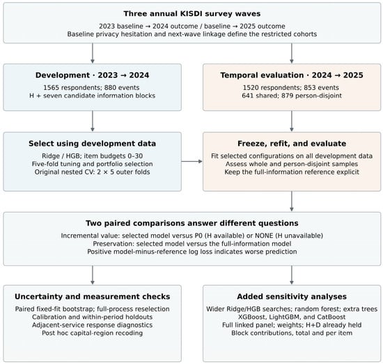
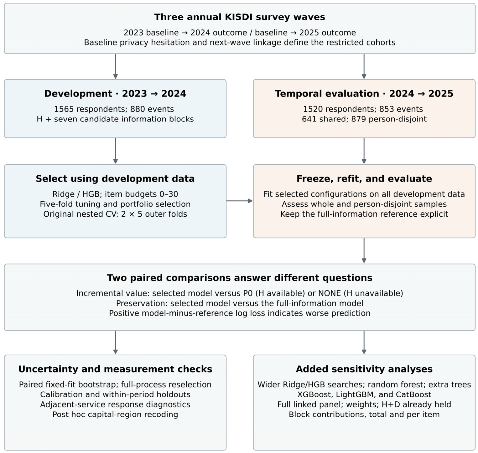
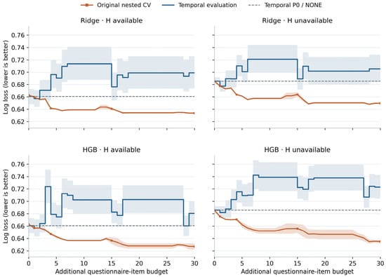
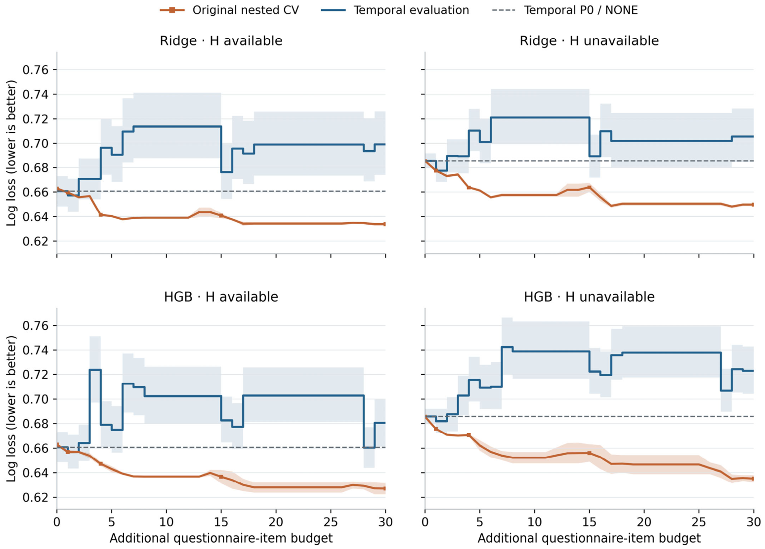
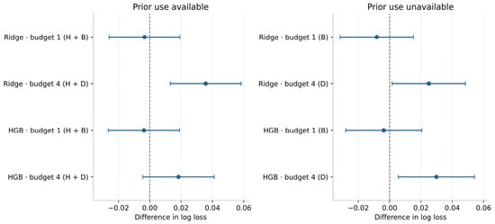
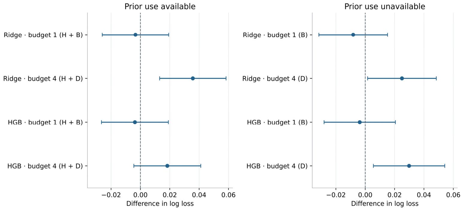
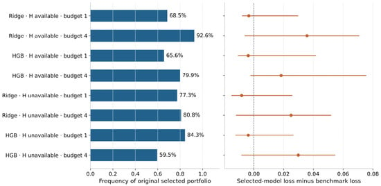
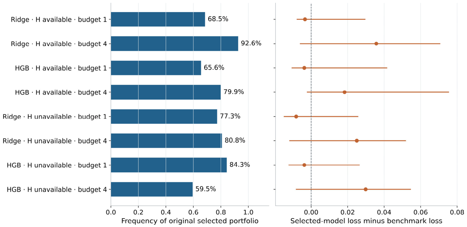
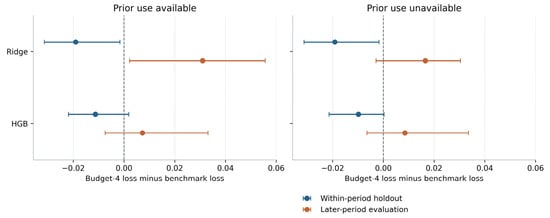
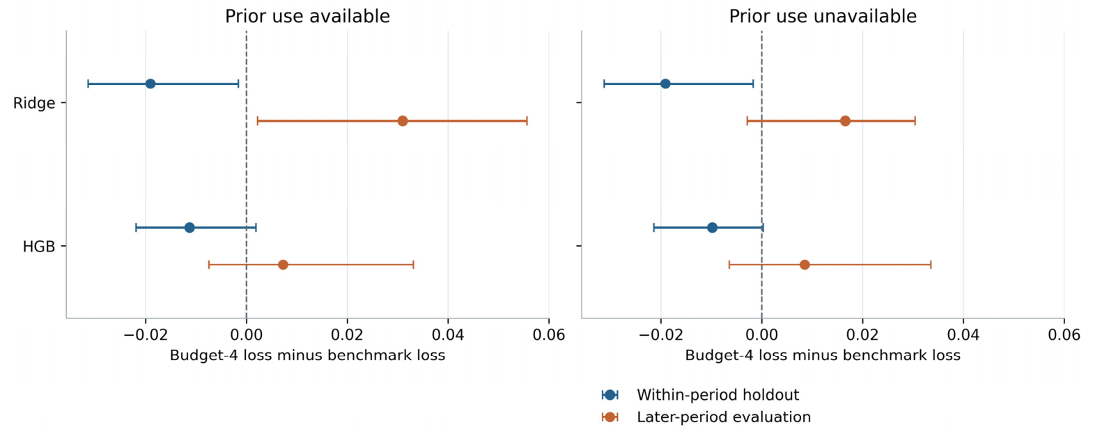
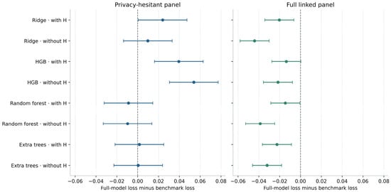
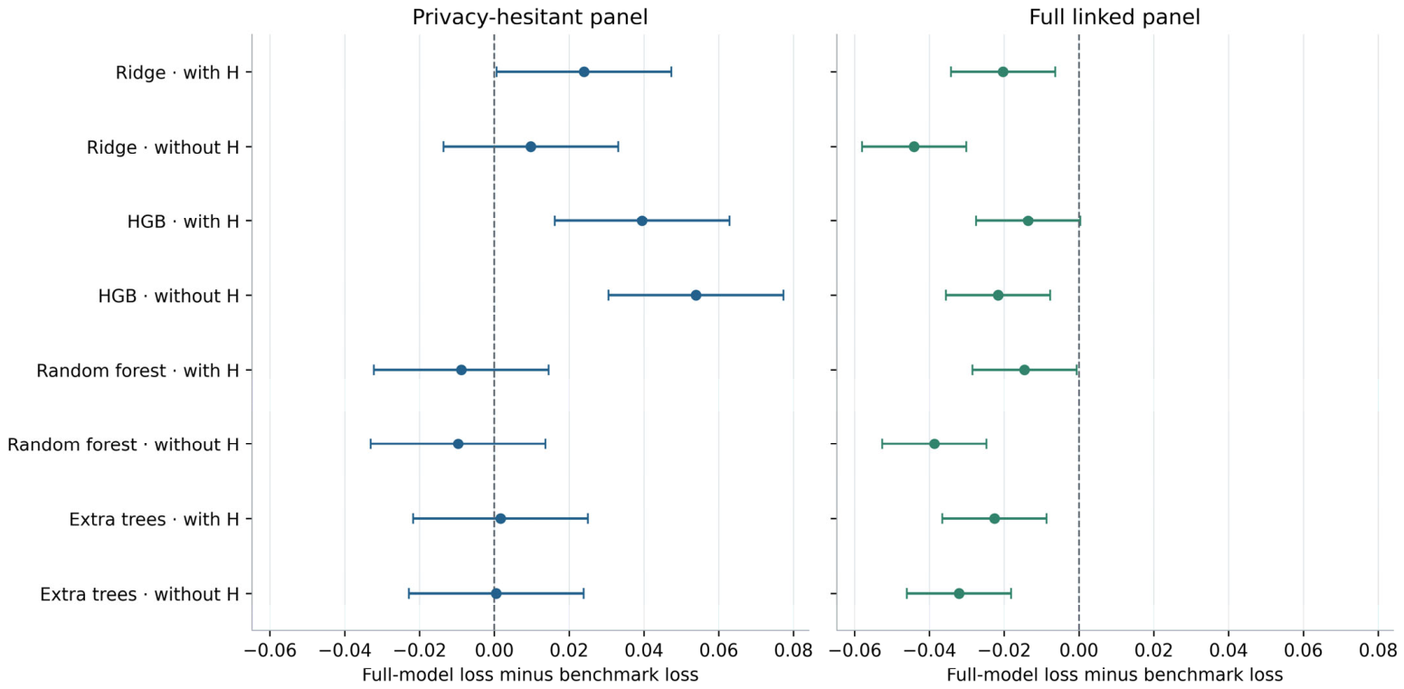
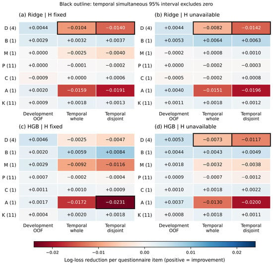
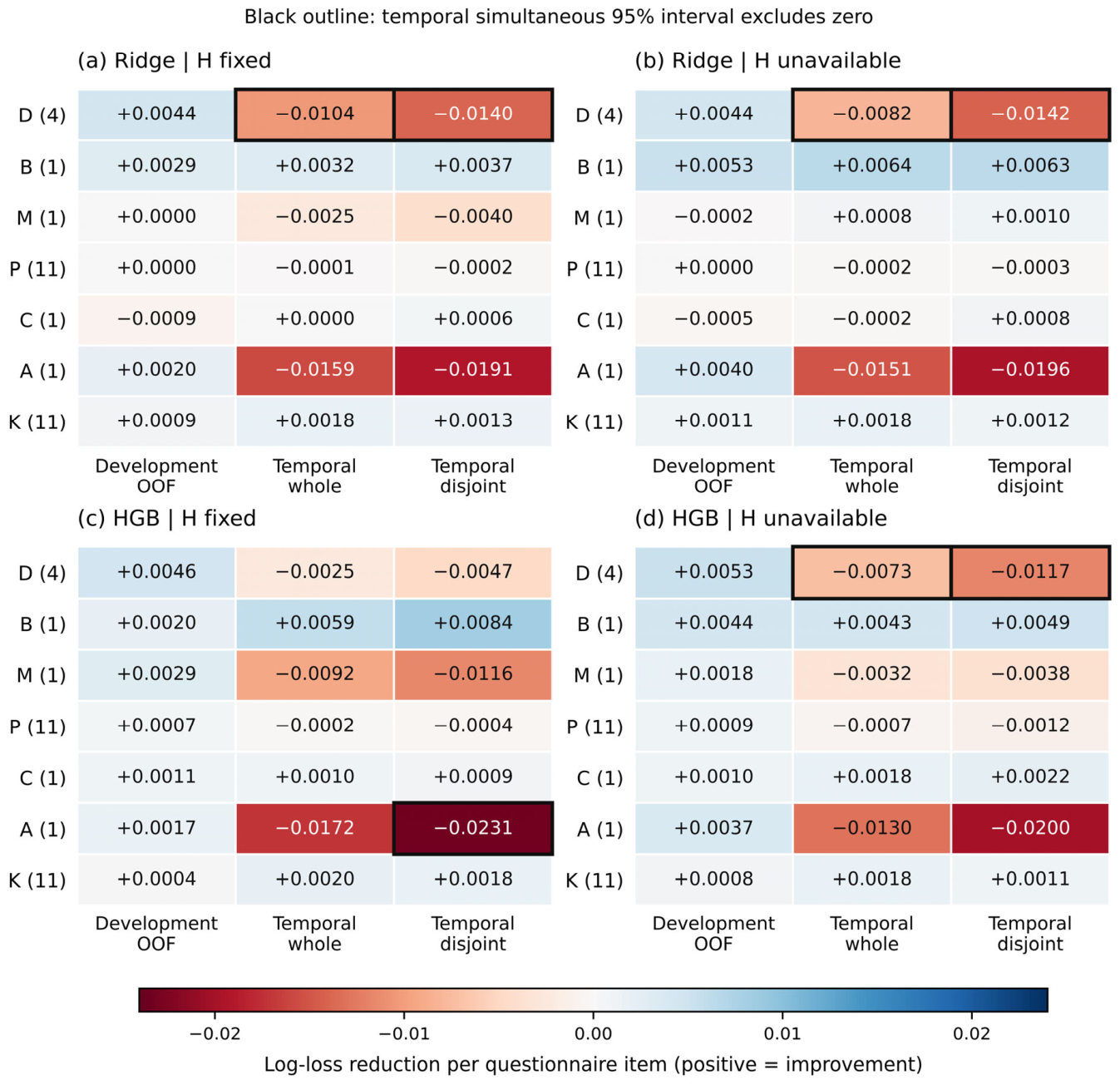

Disclaimer/Publisher’s Note: The statements, opinions and data contained in all publications are solely those of the individual author(s) and contributor(s) and not of MDPI and/or the editor(s). MDPI and/or the editor(s) disclaim responsibility for any injury to people or property resulting from any ideas, methods, instructions or products referred to in the content. |
© 2026 by the authors. Licensee MDPI, Basel, Switzerland. This article is an open access article distributed under the terms and conditions of the Creative Commons Attribution (CC BY) license.